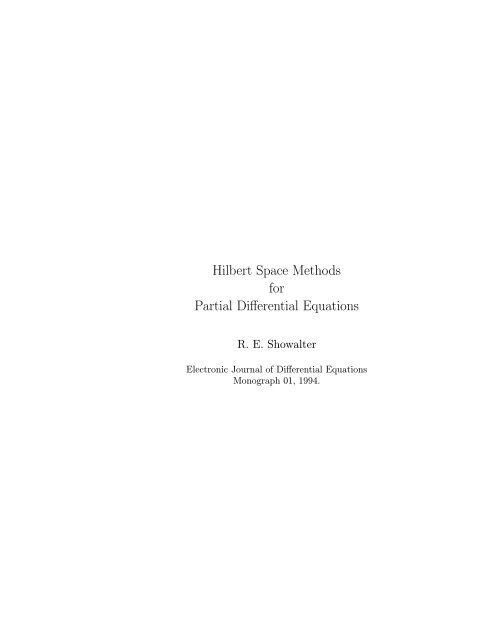
Hilbert Space Methods for Partial Differential Equations

Hilbert Space Methods
for
Partial Differential Equations
R. E. Showalter
Electronic Journal of Differential Equations
Monograph 01, 1994.

i
Preface
This book is an outgrowth of a course which we have given almost periodically
over the last eight years. It is addressed to beginning graduate
students of mathematics, engineering, and the physical sciences. Thus, we
have attempted to present it while presupposing a minimal background: the
reader is assumed to have some prior acquaintance with the concepts of “linear”
and “continuous” and also to believe L 2 is complete. An undergraduate
mathematics training through Lebesgue integration is an ideal background
but we dare not assume it without turning away many of our best students.
The formal prerequisite consists of a good advanced calculus course and a
motivation to study partial differential equations.
A problem is called well-posed if for each set of data there exists exactly
one solution and this dependence of the solution on the data is continuous.
To make this precise we must indicate the space from which the solution
is obtained, the space from which the data may come, and the corresponding
notion of continuity. Our goal in this book is to show that various
types of problems are well-posed. These include boundary value problems
for (stationary) elliptic partial differential equations and initial-boundary
value problems for (time-dependent) equations of parabolic, hyperbolic, and
pseudo-parabolic types. Also, we consider some nonlinear elliptic boundary
value problems, variational or uni-lateral problems, and some methods of
numerical approximation of solutions.
We briefly describe the contents of the various chapters. Chapter I
presents all the elementary Hilbert space theory that is needed for the book.
The first half of Chapter I is presented in a rather brief fashion and is intended
both as a review for some readers and as a study guide for others.
Non-standard items to note here are the spaces C m (Ḡ), V ∗ ,andV ′ . The
first consists of restrictions to the closure of G of functions on R n and the
last two consist of conjugate-linear functionals.
Chapter II is an introduction to distributions and Sobolev spaces. The
latter are the Hilbert spaces in which we shall show various problems are
well-posed. We use a primitive (and non-standard) notion of distribution
which is adequate for our purposes. Our distributions are conjugate-linear
and have the pedagogical advantage of being independent of any discussion
of topological vector space theory.
Chapter III is an exposition of the theory of linear elliptic boundary
value problems in variational form. (The meaning of “variational form” is
explained in Chapter VII.) We present an abstract Green’s theorem which

ii
permits the separation of the abstract problem into a partial differential
equation on the region and a condition on the boundary. This approach has
the pedagogical advantage of making optional the discussion of regularity
theorems. (We construct an operator ∂ which is an extension of the normal
derivative on the boundary, whereas the normal derivative makes sense only
for appropriately regular functions.)
Chapter IV is an exposition of the generation theory of linear semigroups
of contractions and its applications to solve initial-boundary value problems
for partial differential equations. Chapters V and VI provide the immediate
extensions to cover evolution equations of second order and of implicit type.
In addition to the classical heat and wave equations with standard boundary
conditions, the applications in these chapters include a multitude of
non-standard problems such as equations of pseudo-parabolic, Sobolev, viscoelasticity,
degenerate or mixed type; boundary conditions of periodic or
non-local type or with time-derivatives; and certain interface or even global
constraints on solutions. We hope this variety of applications may arouse
the interests even of experts.
Chapter VII begins with some reflections on Chapter III and develops
into an elementary alternative treatment of certain elliptic boundary value
problems by the classical Dirichlet principle. Then we briefly discuss certain
unilateral boundary value problems, optimal control problems, and numerical
approximation methods. This chapter can be read immediately after
Chapter III and it serves as a natural place to begin work on nonlinear
problems.
There are a variety of ways this book can be used as a text. In a year
course for a well-prepared class, one may complete the entire book and supplement
it with some related topics from nonlinear functional analysis. In a
semester course for a class with varied backgrounds, one may cover Chapters
I, II, III, and VII. Similarly, with that same class one could cover in
one semester the first four chapters. In any abbreviated treatment one could
omit I.6, II.4, II.5, III.6, the last three sections of IV, V, and VI, and VII.4.
We have included over 40 examples in the exposition and there are about
200 exercises. The exercises are placed at the ends of the chapters and each
is numbered so as to indicate the section for which it is appropriate.
Some suggestions for further study are arranged by chapter and precede
the Bibliography. If the reader develops the interest to pursue some topic in
one of these references, then this book will have served its purpose.
R. E. Showalter; Austin, Texas, January, 1977.

Contents
I Elements of Hilbert Space 1
1 Linear Algebra . . . . . . . . . . . . . . . . . . . . . . . . . . 1
2 Convergence and Continuity . . . . . . . . . . . . . . . . . . . 6
3 Completeness . . . . . . . . . . . . . . . . . . . . . . . . . . . 10
4 Hilbert Space . . . . . . . . . . . . . . . . . . . . . . . . . . . 14
5 Dual Operators; Identifications . . . . . . . . . . . . . . . . . 19
6 Uniform Boundedness; Weak Compactness . . . . . . . . . . . 22
7 Expansion in Eigenfunctions . . . . . . . . . . . . . . . . . . . 24
II Distributions and Sobolev Spaces 33
1 Distributions . . . . . . . . . . . . . . . . . . . . . . . . . . . 33
2 Sobolev Spaces . . . . . . . . . . . . . . . . . . . . . . . . . . 42
3 Trace . . . . . . . . . . . . . . . . . . . . . . . . . . . . . . . . 47
4 Sobolev’s Lemma and Imbedding . . . . . . . . . . . . . . . . 50
5 Density and Compactness . . . . . . . . . . . . . . . . . . . . 53
IIIBoundary Value Problems 61
1 Introduction . . . . . . . . . . . . . . . . . . . . . . . . . . . . 61
2 Forms, Operators and Green’s Formula . . . . . . . . . . . . . 63
3 Abstract Boundary Value Problems . . . . . . . . . . . . . . . 67
4 Examples . . . . . . . . . . . . . . . . . . . . . . . . . . . . . 69
5 Coercivity; Elliptic Forms . . . . . . . . . . . . . . . . . . . . 76
6 Regularity . . . . . . . . . . . . . . . . . . . . . . . . . . . . . 79
7 Closed operators, adjoints and eigenfunction expansions . . . 85
IV First Order Evolution Equations 97
1 Introduction . . . . . . . . . . . . . . . . . . . . . . . . . . . . 97
2 The Cauchy Problem . . . . . . . . . . . . . . . . . . . . . . . 100
iii

CONTENTS
i
3 Generation of Semigroups . . . . . . . . . . . . . . . . . . . . 102
4 Accretive Operators; two examples . . . . . . . . . . . . . . . 107
5 Generation of Groups; a wave equation . . . . . . . . . . . . . 111
6 Analytic Semigroups . . . . . . . . . . . . . . . . . . . . . . . 115
7 Parabolic Equations . . . . . . . . . . . . . . . . . . . . . . . 121
V Implicit Evolution Equations 129
1 Introduction . . . . . . . . . . . . . . . . . . . . . . . . . . . . 129
2 Regular Equations . . . . . . . . . . . . . . . . . . . . . . . . 130
3 Pseudoparabolic Equations . . . . . . . . . . . . . . . . . . . 134
4 Degenerate Equations . . . . . . . . . . . . . . . . . . . . . . 138
5 Examples . . . . . . . . . . . . . . . . . . . . . . . . . . . . . 140
VI Second Order Evolution Equations 147
1 Introduction . . . . . . . . . . . . . . . . . . . . . . . . . . . . 147
2 Regular Equations . . . . . . . . . . . . . . . . . . . . . . . . 148
3 Sobolev Equations . . . . . . . . . . . . . . . . . . . . . . . . 156
4 Degenerate Equations . . . . . . . . . . . . . . . . . . . . . . 158
5 Examples . . . . . . . . . . . . . . . . . . . . . . . . . . . . . 162
VIIOptimization and Approximation Topics 171
1 Dirichlet’s Principle . . . . . . . . . . . . . . . . . . . . . . . 171
2 Minimization of Convex Functions . . . . . . . . . . . . . . . 172
3 Variational Inequalities . . . . . . . . . . . . . . . . . . . . . . 178
4 Optimal Control of Boundary Value Problems . . . . . . . . . 182
5 Approximation of Elliptic Problems . . . . . . . . . . . . . . 189
6 Approximation of Evolution Equations . . . . . . . . . . . . . 197
VIIISuggested Readings 209

ii
CONTENTS

Chapter I
Elements of Hilbert Space
1 Linear Algebra
We begin with some notation. A function F with domain dom(F )=A
and range Rg(F ) a subset of B is denoted by F : A → B. That a point
x ∈ A is mapped by F to a point F (x) ∈ B is indicated by x ↦→ F (x). If
S is a subset of A then the image of S by F is F (S) ={F(x):x∈S}.
Thus Rg(F )=F(A). The pre-image or inverse image of a set T ⊂ B is
F −1 (T )={x∈A:F(x)∈T}. A function is called injective if it is one-toone,
surjective if it is onto, and bijective if it is both injective and surjective.
Then it is called, respectively, an injection, surjection, orbijection.
K will denote the field of scalars for our vector spaces and is always one
of R (real number system) or C (complex numbers). The choice in most
situations will be clear from the context or immaterial, so we usually avoid
mention of it.
The “strong inclusion” K ⊂⊂ G between subsets of Euclidean space
R n means K is compact, G is open, and K ⊂ G. If A and B are sets,
their Cartesian product is given by A × B = {[a, b] :a∈A, b ∈ B}. If
A and B are subsets of K n (or any other vector space) their set sum is
A + B = {a + b : a ∈ A, b ∈ B}.
1.1
A linear space over the field K is a non-empty set V of vectors with a binary
operation addition +:V×V →V and a scalar multiplication · : K×V → V
1

2 CHAPTER I. ELEMENTS OF HILBERT SPACE
such that (V,+) is an Abelian group, i.e.,
and we have
(x + y)+z=x+(y+z), x,y,z ∈V ,
there is a zero θ ∈ V : x + θ = x, x∈V ,
if x ∈ V ,thereis −x∈V :x+(−x)=θ,and
x + y = y + x , x, y ∈ V ,
(α + β) · x = α · x + β · x,α·(x+y)=α·x+α·y,
α·(β·x)=(αβ) · x, 1·x=x , x, y ∈ V , α,β ∈ K .
We shall suppress the symbol for scalar multiplication since there is no need
for it.
Examples. (a) The set K n of n-tuples of scalars is a linear space over K .
Addition and scalar multiplication are defined coordinatewise:
(x 1 ,x 2 ,...,x n )+(y 1 ,y 2 ,...,y n )=(x 1 +y 1 ,x 2 +y 2 ,...,x n +y n )
α(x 1 ,x 2 ,...,x n )=(αx 1 ,αx 2 ,...,αx n ) .
(b) The set K X of functions f : X → K is a linear space, where X is a
non-empty set, and we define (f 1 + f 2 )(x) =f 1 (x)+f 2 (x), (αf)(x) =αf(x),
x ∈ X.
(c) Let G ⊂ R n be open. The above pointwise definitions of linear operations
give a linear space structure on the set C(G, K) of continuous f : G → K.
We normally shorten this to C(G).
(d) For each n-tuple α =(α 1 ,α 2 ,...,α n ) of non-negative integers, we denote
by D α the partial derivative
∂ |α|
∂x α 1
1 ∂xα 2
2 ···∂xαn n
of order |α| = α 1 + α 2 + ···+α n . The sets C m (G) ={f∈C(G):D α f∈
C(G) for all α, |α| ≤m},m≥0, and C ∞ G = ⋂ m≥1 Cm (G) are linear
spaces with the operations defined above. We let D θ be the identity, where
θ =(0,0,...,0), so C 0 (G) =C(G).
(e) For f ∈ C(G), the support of f is the closure in G of the set {x ∈
G : f(x) ≠0}and we denote it by supp(f). C 0 (G) is the subset of those
functions in C(G) with compact support. Similarly, we define C0 m(G) =
C m (G)∩C 0 (G), m ≥ 1andC0 ∞(G)=C∞ (G)∩C 0 (G).

1. LINEAR ALGEBRA 3
(f) If f : A → B and C ⊂ A, wedenotef| C the restriction of f to C. We
obtain useful linear spaces of functions on the closure Ḡ as follows:
C m (Ḡ) ={f|Ḡ:f∈Cm 0 (Rn )} , C ∞ (Ḡ)={f|Ḡ:f∈C∞ 0 (Rn )}.
These spaces play a central role in our work below.
1.2
A subset M of the linear space V is a subspace of V if it is closed under the
linear operations. That is, x + y ∈ M whenever x, y ∈ M and αx ∈ M for
each α ∈ K and x ∈ M. We denote that M is a subspace of V by M ≤ V .
It follows that M is then (and only then) a linear space with addition and
scalar multiplication inherited from V .
Examples. We have three chains of subspaces given by
C j (G) ≤ C k (G) ≤ K G ,
Cj (Ḡ) ≤ Ck (Ḡ) , and
{θ} ≤ C j 0 (G) ≤ Ck 0 (G) , 0 ≤ k ≤ j ≤∞.
Moreover, for each k as above, we can identify ϕ ∈ C0 k (G) withthatΦ∈
Ck (Ḡ) obtained by defining Φ to be equal to ϕ on G and zero on ∂G, the
boundary of G. Likewise we can identify each Φ ∈ C k (Ḡ)withΦ| G ∈C K (G).
These identifications are “compatible” and we have C0 k (G) ≤ Ck (Ḡ) ≤
C k (G).
1.3
We let M be a subspace of V and construct a corresponding quotient space.
For each x ∈ V , define a coset ˆx = {y ∈ V : y − x ∈ M } = {x + m : m ∈ M }.
The set V/M = {ˆx : x ∈ V} is the quotient set. Anyy∈ˆxis a representative
of the coset ˆx and we clearly have y ∈ ˆx if and only if x ∈ ŷ if and only if
ˆx =ŷ. We shall define addition of cosets by adding a corresponding pair of
representatives and similarly define scalar multiplication. It is necessary to
first verify that this definition is unambiguous.
Lemma If x 1 ,x 2 ∈ ˆx, y 1 ,y 2 ∈ ŷ,andα∈K,then (x1 ̂+y 1 )= (x2 ̂+y 2 )
and (αx ̂ 1 )=(αx ̂ 2 ).

4 CHAPTER I. ELEMENTS OF HILBERT SPACE
The proof follows easily, since M is closed under addition and scalar multiplication,
and we can define ˆx +ŷ= (x+y)andαˆx= ̂
(αx). ̂ These operations
make V/M a linear space.
Examples. (a) Let V = R 2 and M = {(0,x 2 ):x 2 ∈R}. Then V/M is
the set of parallel translates of the x 2 -axis, M, and addition of two cosets is
easily obtained by adding their (unique) representatives on the x 1 -axis.
(b) Take V = C(G). Let x 0 ∈ G and M = {ϕ ∈ C(G) :ϕ(x 0 )=0}. Write
each ϕ ∈ V in the form ϕ(x) =(ϕ(x)−ϕ(x 0 )) + ϕ(x 0 ). This representation
can be used to show that V/M is essentially equivalent (isomorphic) to K.
(c) Let V = C(Ḡ) andM=C 0(G). We can describe V/M as a space of
“boundary values.” To do this, begin by noting that for each K ⊂⊂ G there
is a ψ ∈ C 0 (G) withψ=1onK. (Cf. Section II.1.1.) Then write a given
ϕ ∈ C(Ḡ) intheform ϕ=(ϕψ)+ϕ(1 − ψ) ,
where the first term belongs to M and the second equals ϕ in a neighborhood
of ∂G.
1.4
Let V and W be linear spaces over K. A function T : V → W is linear if
T (αx + βy) =αT (x)+βT(y) , α,β ∈ K , x,y ∈ V .
That is, linear functions are those which preserve the linear operations. An
isomorphism is a linear bijection. The set {x ∈ V : Tx =0}is called the
kernel of the (not necessarily linear) function T : V → W and we denote it
by K(T ).
Lemma If T : V → W is linear, then K(T ) is a subspace of V , Rg(T ) is
a subspace of W ,andK(T)={θ}if and only if T is an injection.
Examples. (a) Let M be a subspace of V . The identity i M : M → V is a
linear injection x ↦→ x and its range is M.
(b) The quotient map q M : V → V/M, x ↦→ ˆx, is a linear surjection with
kernel K(q M )=M.
(c) Let G be the open interval (a, b) inRand consider D ≡ d/dx: V → C(Ḡ),
where V is a subspace of C1 (Ḡ). If V = C1 (Ḡ), then D is a linear surjection
with K(D) consisting of constant functions on Ḡ. If V = {ϕ ∈ C1 (Ḡ):

1. LINEAR ALGEBRA 5
ϕ(a) =0},thenDis an isomorphism. Finally, if V = {ϕ ∈ C1 (Ḡ) :ϕ(a)=
ϕ(b)=0},thenRg(D)={ϕ∈C(Ḡ):∫ b
a ϕ=0}.
Our next result shows how each linear function can be factored into the
product of a linear injection and an appropriate quotient map.
Theorem 1.1 Let T : V → W be linear and M be a subspace of K(T ).
Then there is exactly one function ̂T : V/M → W for which ̂T ◦ q M = T ,
and ̂T is linear with Rg( ̂T )=Rg(T). Finally, ̂T is injective if and only if
M = K(T ).
Proof : Ifx 1 ,x 2 ∈ ˆx,thenx 1 −x 2 ∈M⊂K(T), so T (x 1 )=T(x 2 ). Thus we
can define a function as desired by the formula ̂T (ˆx)=T(x). The uniqueness
and linearity of ̂T follow since q M is surjective and linear. The equality of
the ranges follows, since q M is surjective, and the last statement follows from
the observation that K(T ) ⊂ M if and only if v ∈ V and ̂T (ˆx) =0imply
ˆx=ˆ0.
An immediate corollary is that each linear function T : V → W can be
factored into a product of a surjection, an isomorphism, and an injection:
T = i Rg(T ) ◦ ̂T ◦ q K(T ) .
A function T : V → W is called conjugate linear if
T (αx + βy) =ᾱT (x)+ ¯βT(y) , α,β ∈ K , x,y ∈ V .
Results similar to those above hold for such functions.
1.5
Let V and W be linear spaces over K and consider the set L(V,W) of linear
functions from V to W .ThesetW V of all functions from V to W is a linear
space under the pointwise definitions of addition and scalar multiplication
(cf. Example 1.1(b)), and L(V,W) is a subspace.
We define V ∗ to be the linear space of all conjugate linear functionals
from V → K. V ∗ is called the algebraic dual of V . Note that there is
a bijection f ↦→ ¯f of L(V,K) ontoV ∗ , where ¯f is the functional defined
by ¯f (x) = f(x) for x ∈ V and is called the conjugate of the functional
f : V → K. Such spaces provide a useful means of constructing large linear
spaces containing a given class of functions. We illustrate this technique in
a simple situation.

6 CHAPTER I. ELEMENTS OF HILBERT SPACE
Example. Let G be open in R n and x 0 ∈ G. We shall imbed the space
C(G) in the algebraic dual of C 0 (G). For each f ∈ C(G), define T f ∈ C 0 (G) ∗
by
∫
T f (ϕ) = f¯ϕ, ϕ∈C 0 (G).
G
Since f ¯ϕ ∈ C 0 (G), the Riemann integral is adequate here. An easy exercise
shows that the function f ↦→ T f : C(G) → C 0 (G) ∗ is a linear injection, so we
may thus identify C(G) with a subspace of C 0 (G) ∗ . This linear injection is
not surjective; we can exhibit functionals on C 0 (G) which are not identified
with functions in C(G). In particular, the Dirac functional δ x0 defined by
δ x0 (ϕ) =ϕ(x 0 ), ϕ ∈ C 0 (G) ,
cannot be obtained as T f for any f ∈ C(G). That is, T f = δ x0 implies that
f(x) = 0 for all x ∈ G, x ≠ x 0 , and thus f = 0, a contradiction.
2 Convergence and Continuity
The absolute value function on R and modulus function on C are denoted
by |·|, and each gives a notion of length or distance in the corresponding
space and permits the discussion of convergence of sequences in that space
or continuity of functions on that space. We shall extend these concepts to
a general linear space.
2.1
A seminorm on the linear space V is a function p : V → R for which
p(αx) =|α|p(x)andp(x+y)≤p(x)+p(y) for all α ∈ K and x, y ∈ V .The
pair V,p is called a seminormed space.
Lemma 2.1 If V,p is a seminormed space, then
(a) |p(x) − p(y)| ≤p(x−y), x,y ∈ V ,
(b) p(x) ≥ 0 ,
x ∈ V ,and
(c) the kernel K(p) is a subspace of V .
(d) If T ∈ L(W, V ), thenp◦T:W→Ris a seminorm on W .

2. CONVERGENCE AND CONTINUITY 7
(e) If p j is a seminorm on V and α j ≥ 0, 1 ≤ j ≤ n, then ∑ n
j=1 α j p j is a
seminorm on V .
Proof : Wehavep(x)=p(x−y+y)≤p(x−y)+p(y)sop(x)−p(y)≤p(x−y).
Similarly, p(y) − p(x) ≤ p(y − x) =p(x−y), so the result follows. Setting
y = 0 in (a) and noting p(0) = 0, we obtain (b). The result (c) follows
directly from the definitions, and (d) and (e) are straightforward exercises.
If p is a seminorm with the property that p(x) > 0foreachx≠θ,we
call it a norm.
Examples. (a) For 1 ≤ k ≤ n we define seminorms on K n by p k (x) =
∑ kj=1
|x j |, q k (x) =( ∑ k
j=1 |x j | 2 ) 1/2 ,andr k (x)=max{|x j | :1≤j≤k}.Each
of p n , q n and r n is a norm.
(b) If J ⊂ X and f ∈ K X , we define p J (f) =sup{|f(x)| : x ∈ J}. Then
for each finite J ⊂ X, p J is a seminorm on K X .
(c) For each K ⊂⊂ G, p K is a seminorm on C(G). Also, p = p Ḡ G is a
norm on C(Ḡ).
(d) For each j, 0≤j≤k,andK⊂⊂ G we can define a seminorm on
C k (G) byp j,K (f) =sup{|D α f(x)| : x ∈ K, |α| ≤j}. Each such p j,G is a
norm on C k (Ḡ).
2.2
Seminorms permit a discussion of convergence. We say the sequence {x n }
in V converges to x ∈ V if lim n→∞ p(x n − x) = 0; that is, if {p(x n − x)} is
a sequence in R converging to 0. Formally, this means that for every ε>0
there is an integer N ≥ 0 such that p(x n − x)

8 CHAPTER I. ELEMENTS OF HILBERT SPACE
0 which shows that (x n + y n ) → x + y. Sincex n +y n ∈M,alln, this implies
that x+y ∈ ¯M. Similarly, for α ∈ K we have p(αx−αx n )=|α|p(x−x n )→0,
so αx ∈ ¯M.
2.3
Let V,p and W, q be seminormed spaces and T : V → W (not necessarily
linear). Then T is called continuous at x ∈ V if for every ε>0thereisa
δ>0forwhichy∈V and p(x − y) 0 as in the definition
above and then N such that n ≥ N implies p(x n − x)

2. CONVERGENCE AND CONTINUITY 9
(b) the identity I : V,p → V,q is continuous, and
(c) there is a constant K ≥ 0 such that
q(x) ≤ Kp(x) , x ∈ V .
Proof : By Theorem 2.2, (a) is equivalent to having the identity I : V,p → V,q
continuous at 0, so (b) implies (a). If (c) holds, then q(x − y) ≤ Kp(x − y),
x, y ∈ V , so (b) is true.
We claim now that (a) implies (c). If (c) is false, then for every integer
n ≥ 1thereisanx n ∈V for which q(x n ) >np(x n ). Setting y n =
(1/q(x n ))x n , n ≥ 1, we have obtained a sequence for which q(y n )=1 and
p(y n )→0, thereby contradicting (a).
Theorem 2.4 Let V,p and W, q be seminormed spaces and T ∈ L(V,W).
The following are equivalent:
(a) T is continuous at θ ∈ V ,
(b) T is continuous, and
(c) there is a constant K ≥ 0 such that
q(T (x)) ≤ Kp(x) , x ∈ V .
Proof : By Theorem 2.3, each of these is equivalent to requiring that the
seminorm p be stronger than the seminorm q ◦ T on V .
2.4
If V,p and W, q are seminormed spaces, we denote by L(V,W) thesetof
continuous linear functions from V to W . This is a subspace of L(V,W)
whose elements are frequently called the bounded operators from V to W
(because of Theorem 2.4).
Let T ∈L(V,W) and consider
λ ≡ sup{q(T (x)) : x ∈ V , p(x) ≤ 1} ,
µ ≡ inf{K >0:q(T(x)) ≤ Kp(x) for all x ∈ V } .

10 CHAPTER I. ELEMENTS OF HILBERT SPACE
If K belongs to the set defining µ, then for every x ∈ V : p(x) ≤ 1we
have q(T (x)) ≤ K, hence λ ≤ K. This holds for all such K, soλ≤µ. If
x ∈ V with p(x) > 0, then y ≡ (1/p(x))x satisfies p(y) =1,soq(T(y)) ≤ λ.
That is q(T (x)) ≤ λp(x) whenever p(x) > 0. But by Theorem 2.4(c) this
last inequality is trivially satisfied when p(x) =0,sowehaveµ≤λ.These
remarks prove the first part of the following result; the remaining parts are
straightforward.
Theorem 2.5 Let V,p and W, q be seminormed spaces. For each T ∈
L(V,W) we define a real number by |T | p,q ≡ sup{q(T (x)) : x ∈ V , p(x) ≤ 1}.
Then we have |T | p,q =sup{q(T(x)) : x ∈ V , p(x) =1}=inf{K > 0:
q(T(x)) ≤ Kp(x) for all x ∈ V } and |·| p,q is a seminorm on L(V,W). Furthermore,
q(T (x)) ≤|T| p,q · p(x), x ∈ V ,and|·| p,q is a norm whenever q is
a norm.
Definitions. The dual of the seminormed space V,p is the linear space
V ′ = {f ∈ V ∗ : f is continuous} with the norm
‖f‖ V ′ =sup{|f(x)| : x ∈ V , p(x) ≤ 1} .
If V,p and W, q are seminormed spaces, then T ∈L(V,W) is called a contraction
if |T | p,q ≤ 1, and T is called an isometry if |T | p,q =1.
3 Completeness
3.1
A sequence {x n } in a seminormed space V,p is called Cauchy if lim m,n→∞ p(x m
− x n ) = 0, that is, if for every ε>0 there is an integer N such that
p(x m − x n )

3. COMPLETENESS 11
For m ≥ n we have p(x m − x n ) ≤ 1/n, so{x m }is Cauchy. If x ∈ C(Ḡ), then
∫ c−1/n
∫ 1
p(x n − x) ≥ |x(t)| dt + |1 − x(t)| d(t) .
0
c
This shows that if {x n } converges to x then x(t) =0for0≤t

12 CHAPTER I. ELEMENTS OF HILBERT SPACE
3.3
A completion of the seminormed space V,p is a complete seminormed space
W, q and a linear injection T : V → W for which Rg(T )isdenseinW and T
preserves seminorms: q(T (x)) = p(x) for all x ∈ V . By identifying V,p with
Rg(T ),q, we may visualize V as being dense and contained in a corresponding
space that is complete. The completion of a normed space is a Banach
space and linear injection as above. If two Banach spaces are completions
of a given normed space, then we can use Theorem 3.1 to construct a linear
norm-preserving bijection between them, so the completion of a normed
space is essentially unique.
We first construct a completion of a given seminormed space V,p. Let
W be the set of all Cauchy sequences in V,p. From the estimate |p(x n ) −
p(x m )| ≤ p(x n − x m ) it follows that ¯p({x n }) = lim n→∞ p(x n ) defines a
function ¯p : W → R and it easily follows that ¯p is a seminorm on W . For
each x ∈ V ,letTx = {x,x,x,...}, the indicated constant sequence. Then
T : V,p → W, ¯p is a linear seminorm-preserving injection. If {x n }∈W,
then for any ε>0 there is an integer N such that p(x n − x N )

3. COMPLETENESS 13
Theorem 3.3 Let V,p be a seminormed space, M a subspace of V and
define
ˆp(ˆx)=inf{p(y):y∈ˆx}, ˆx∈V/M .
(a) V/M, ˆp is a seminormed space and the quotient map q : V → V/M has
(p, ˆp)-seminorm =1.
(b) If D is dense in V ,then ˆD={ˆx:x∈D}is dense in V/M.
(c) ˆp is a norm if and only if M is closed.
(d) If V,p is complete, then V/M, ˆp is complete.
Proof : We leave (a) and (b) as exercises. Part (c) follows from the observation
that ˆp(ˆx) = 0 if and only if x ∈ ¯M.
To prove (d), we recall that a Cauchy sequence converges if it has a
convergent subsequence so we need only consider a sequence {ˆx n } in V/M
for which ˆp(ˆx n+1 − ˆx n ) < 1/2 n , n ≥ 1. For each n ≥ 1wepicky n ∈ˆx n with
p(y n+1 − y n ) < 1/2 n .Form≥nwe obtain
p(y m − y n ) ≤
m−1−n ∑
k=0
p(y n+1+k − y n+k ) <
∞∑
2 −(n+k) =2 1−n .
Thus {y n } is Cauchy in V,p and part (a) shows ˆx n → ˆx in V/M,wherexis
the limit of {y n } in V,p.
Given V,p and the completion W, ¯p constructed for Theorem 3.2, we
consider the quotient space W/K and its corresponding seminorm ˆp, where
Kis the kernel of ¯p. The continuity of ¯p : W → R implies that K is closed,
so ˆp is a norm on W/K. W, ¯p is complete, so W/K, ˆpis a Banach space.
The quotient map q : W → W/K satisfies ˆp(q(x)) = ˆp(ˆx) = ¯p(y) for all
y ∈ q(x), so q preserves the seminorms. Since Rg(T )isdenseinW it follows
that the linear map q ◦ T : V → W/K has a dense range in W/K. Wehave
ˆp((q ◦T )x) =ˆp(̂Tx)=p(x)forx∈V, hence K(q ◦T ) ≤ K(p). If p is a norm
this shows that q ◦ T is injective and proves the following.
k=0
Theorem 3.4 Every normed space has a completion.

14 CHAPTER I. ELEMENTS OF HILBERT SPACE
3.5
We briefly consider the vector space L(V,W).
Theorem 3.5 If V,p is a seminormed space and W, q is a Banach space,
then L(V,W) is a Banach space. In particular, the dual V ′ of a seminormed
space is complete.
Proof : Let {T n } be a Cauchy sequence in L(V,W). For each x ∈ V ,the
estimate
q(T m x − T n x) ≤|T m −T n |p(x)
shows that {T n x} is Cauchy, hence convergent to a unique T (x) ∈ W .This
defines T : V → W and the continuity of addition and scalar multiplication
in W will imply that T ∈ L(V,W). We have
q(T n (x)) ≤|T n |p(x), x ∈ V ,
and {|T n |} is Cauchy, hence, bounded in R, so the continuity of q shows that
T ∈L(V,W) with|T|≤K≡sup{|T n | : n ≥ 1}.
To show T n → T in L(V,W), let ε>0andchooseNso large that
m, n ≥ N implies |T m − T n |

4. HILBERT SPACE 15
Theorem 4.1 If V,(·,·) is a scalar product space, then
(a) |(x, y)| 2 ≤ (x, x) · (y,y) , x,y ∈ V ,
(b) ‖x‖ ≡(x, x) 1/2 defines a norm ‖·‖ on V for which
‖x + y‖ 2 + ‖x − y‖ 2 =2(‖x‖ 2 +‖y‖ 2 ), x,y ∈ V , and
(c) the scalar product is continuous from V × V to K.
Proof :
Part (a) follows from the computation
0 ≤ (αx + βy,αx + βy) =β(β(y,y) −|α| 2 )
for the scalars α = −(x, y) andβ=(x, x). To prove (b), we use (a) to verify
‖x + y‖ 2 ≤‖x‖ 2 +2|(x, y)| + ‖y‖ 2 ≤ (‖x‖ + ‖y‖) 2 .
The remaining norm axioms are easy and the indicated identity is easily
verified. Part (c) follows from the estimate
|(x, y) − (x n ,y n )|≤‖x‖‖y−y n ‖+‖y n ‖‖x−x n ‖
applied to a pair of sequences, x n → x and y n → y in V,‖·‖.
A Hilbert space is a scalar product space for which the corresponding
normed space is complete.
Examples. (a) Let V = K N with vectors x =(x 1 ,x 2 ,...,x N ) and define
(x, y) = ∑ N
j=1 x j ȳ j . Then V,(·,·) is a Hilbert space (with the norm ‖x‖ =
( ∑ N
j=1 |x j | 2 ) 1/2 ) which we refer to as Euclidean space.
(b)WedefineC 0 (G) a scalar product by
∫
(ϕ, ψ) = ϕ¯ψ
where G is open in R n and the Riemann integral is used. This scalar product
space is not complete.
(c) On the space L 2 (G) of (equivalence classes of) Lebesgue squaresummable
K-valued functions we define the scalar product as in (b) but
with the Lebesgue integral. This gives a Hilbert space in which C 0 (G) isa
dense subspace.
G

16 CHAPTER I. ELEMENTS OF HILBERT SPACE
Suppose V,(·,·) is a scalar product space and let B,‖ ·‖ denote the
completion of V,‖ ·‖. For each y ∈ V, the function x ↦→ (x, y) is linear,
hence has a unique extension to B, thereby extending the definition of (x, y)
to B × V .Itiseasytoverifythatforeachx∈B, the function y ↦→ (x, y) is
in V ′ and we can similarly extend it to define (x, y) onB×B.Bychecking
that (the extended) function (·, ·) is a scalar product on B, wehaveproved
the following result.
Theorem 4.2 Every scalar product space has a (unique) completion which
is a Hilbert space and whose scalar product is the extension by continuity of
the given scalar product.
Example. L 2 (G) is the completion of C 0 (G) with the scalar product given
above.
4.2
The scalar product gives us a notion of angles between vectors. (In particular,
recall the formula (x, y) =‖x‖‖y‖cos(θ) in Example (a) above.) We
call the vectors x, y orthogonal if (x, y) = 0. For a given subset M of the
scalar product space V , we define the orthogonal complement of M to be
the set
M ⊥ = {x ∈ V :(x, y) = 0 for all y ∈ M} .
Lemma M ⊥ is a closed subspace of V and M ∩ M ⊥ = {0}.
Proof : For each y ∈ M,theset{x∈V :(x, y) =0}is a closed subspace
and so then is the intersection of all these for y ∈ M. The only vector
orthogonal to itself is the zero vector, so the second statement follows.
AsetKin the vector space V is convex if for x, y ∈ K and 0 ≤ α ≤ 1,
we have αx +(1−α)y ∈K. That is, if a pair of vectors is in K, thensoalso
is the line segment joining them.
Theorem 4.3 A non-empty closed convex subset K of the Hilbert space H
has an element of minimal norm.
Proof : Setting d ≡ inf{‖x‖ : x ∈ K}, we can find a sequence x n ∈ K
for which ‖x n ‖→d. Since K is convex we have (1/2)(x n + x m ) ∈ K for

4. HILBERT SPACE 17
m, n ≥ 1, hence ‖x n + x m ‖ 2 ≥ 4d 2 . From Theorem 4.1(b) we obtain the
estimate ‖x n − x m ‖ 2 ≤ 2(‖x n ‖ 2 + ‖x m ‖ 2 ) − 4d 2 . The right side of this
inequality converges to 0, so {x n } is Cauchy, hence, convergent to some
x ∈ H. K is closed, so x ∈ K, and the continuity of the norm shows that
‖x‖ = lim n ‖x n ‖ = d.
We note that the element with minimal norm is unique, for if y ∈ K with
‖y‖ = d, then(1/2)(x + y) ∈ K and Theorem 4.1(b) give us, respectively,
4d 2 ≤‖x+y‖ 2 =4d 2 −‖x−y‖ 2 .Thatis,‖x−y‖=0.
Theorem 4.4 Let M be a closed subspace of the Hilbert space H. Then for
every x ∈ H we have x = m + n, wherem∈Mand n ∈ M ⊥ are uniquely
determined by x.
Proof : The uniqueness follows easily, since if x = m 1 + n 1 with m 1 ∈ M,
n 1 ∈ M ⊥ ,thenm 1 −m=n−n 1 ∈M∩M ⊥ ={θ}. To establish the
existence of such a pair, define K = {x + y : y ∈ M} and use Theorem 4.3
to find n ∈ K with ‖n‖ =inf{‖x + y‖ : y ∈ M}. Then set m = x −n. It
is clear that m ∈ M and we need only to verify that n ∈ M ⊥ . Let y ∈ M.
For each α ∈ K, wehaven−αy ∈ K, hence ‖n − αy‖ 2 ≥‖n‖ 2 . Setting
α = β(n, y), β>0, gives us |(n, y)| 2 (β‖y‖ 2 − 2) ≥ 0, and this can hold for
all β>0onlyif(n, y) =0.
4.3
From Theorem 4.4 it follows that for each closed subspace M of a Hilbert
space H we can define a function P M : H → M by P M : x = m + n ↦→ m,
where m ∈ M and n ∈ M ⊥ as above. The linearity of P M is immediate and
the computation
‖P M x‖ 2 ≤‖P M x‖ 2 +‖n‖ 2 =‖P M x+n‖ 2 =‖x‖ 2
shows P M ∈L(H, H) with‖P M ‖≤1. Also, P M x = x exactly when x ∈ M,
so P M ◦ P M = P M . The operator P M is called the projection on M.
If P ∈L(B,B) satisfiesP◦P=P,thenP is called a projection on the
Banach space B. The result of Theorem 4.4 is a guarantee of a rich supply
of projections in a Hilbert space.

18 CHAPTER I. ELEMENTS OF HILBERT SPACE
4.4
We recall that the (continuous) dual of a seminormed space is a Banach
space. We shall show there is a natural correspondence between a Hilbert
space H and its dual H ′ . Consider for each fixed x ∈ H the function f x
defined by the scalar product: f x (y) =(x, y), y ∈ H. It is easy to check
that f x ∈ H ′ and ‖f x ‖ H ′ = ‖x‖. Furthermore, the map x ↦→ f x : H → H ′ is
linear:
f x+z = f x + f z , x,z ∈ H,
f αx = αf x , α ∈ K , x ∈ H.
Finally, the function x ↦→ f x : H → H ′ is a norm preserving and linear
injection. The above also holds in any scalar product space, but for Hilbert
spaces this function is also surjective. This follows from the next result.
Theorem 4.5 Let H be a Hilbert space and f ∈ H ′ .
element x ∈ H (and only one) for which
Then there is an
f(y) =(x, y) , y ∈ H.
Proof : We need only verify the existence of x ∈ H. Iff=θwe take x = θ,
so assume f ≠ θ in H ′ . Then the kernel of f, K = {x ∈ H : f(x) =0}is a
closed subspace of H with K ⊥ ≠ {θ}. Letn∈K ⊥ be chosen with ‖n‖ =1.
For each z ∈ K ⊥ it follows that f(n)z − f(z)n ∈ K ∩ K ⊥ = {θ}, sozis a
scalar multiple of n. (Thatis,K ⊥ is one-dimensional.) Thus, each y ∈ H is
of the form y = P K (y)+λn where (y,n) =λ(n, n) =λ. But we also have
f(y) =¯λf(n), since P K (y) ∈ K, and thus f(y) =(f(n)n, y) for all y ∈ H.
The function x ↦→ f x from H to H ′ will occur frequently in our later
discussions and it is called the Riesz map and is denoted by R H .Notethat
it depends on the scalar product as well as the space. In particular, R H is
an isometry of H onto H ′ defined by
R H (x)(y) =(x, y) H , x,y ∈ H.

5. DUAL OPERATORS; IDENTIFICATIONS 19
5 Dual Operators; Identifications
5.1
Suppose V and W are linear spaces and T ∈ L(V,W). Then we define the
dual operator T ′ ∈ L(W ∗ ,V ∗ )by
T ′ (f)=f◦T, f∈W ∗ .
Theorem 5.1 If V is a linear space, W, q is a seminorm space, and T ∈
L(V,W) has dense range, then T ′ is injective on W ′ . If V,p and W, q are
seminorm spaces and T ∈L(V,W), then the restriction of the dual T ′ to W ′
belongs to L(W ′ ,V ′ ) and it satisfies
‖T ′ ‖ L(W ′ ,V ′ ) ≤|T| p,q .
Proof : The first part follows from Section 3.2. The second is obtained from
the estimate
|T ′ f(x)| ≤‖f‖ W ′|T| p,q p(x) , f ∈ W ′ , x ∈ V .
We give two basic examples. Let V be a subspace of the seminorm space
W, q and let i : V → W be the identity. Then i ′ (f) =f◦iis the restriction
of f to the subspace V ; i ′ is injective on W ′ if (and only if) V is dense in
W . In such cases we may actually identify i ′ (W ′ )withW ′ , and we denote
this identification by W ′ ≤ V ∗ .
Consider the quotient map q : W → W/V where V and W, q are given
as above. It is clear that if g ∈ (W/V ) ∗ and f = q ′ (g), i.e., f = g ◦ q, then
f∈W ∗ and V ≤ K(f). Conversely, if f ∈ W ∗ and V ≤ K(f), then Theorem
1.1 shows there is a g ∈ (W/V ) ∗ for which q ′ (g) =f. These remarks show
that Rg(q ′ )={f∈W ∗ :V ≤K(f)}. Finally, we note by Theorem 3.3 that
|q| q,ˆq = 1, so it follows that g ∈ (W, V ) ′ if and only if q ′ (g) ∈ W ′ .
5.2
Let V and W be Hilbert spaces and T ∈L(V,W). We define the adjoint of
T as follows: if u ∈ W , then the functional v ↦→ (u, T v) W belongs to V ′ ,so
Theorem 4.5 shows that there is a unique T ∗ u ∈ V such that
(T ∗ u, v) V =(u, T v) W , u ∈ W,v∈V .

20 CHAPTER I. ELEMENTS OF HILBERT SPACE
Theorem 5.2 If V and W are Hilbert spaces and T ∈L(V,W), thenT ∗ ∈
L(W, V ), Rg(T ) ⊥ = K(T ∗ ) and Rg(T ∗ ) ⊥ = K(T ). If T is an isomorphism
with T −1 ∈L(W, V ), thenT ∗ is an isomorphism and (T ∗ ) −1 =(T −1 ) ∗ .
We leave the proof as an exercise and proceed to show that dual operators
are essentially equivalent to the corresponding adjoint. Let V and W be
Hilbert spaces and denote by R V and R W the corresponding Riesz maps (Section
4.4) onto their respective dual spaces. Let T ∈L(V,W) and consider its
dual T ′ ∈L(W ′ ,V ′ ) and its adjoint T ∗ ∈L(W, V ). For u ∈ W and v ∈ V we
have R V ◦T ∗ (u)(v) =(T ∗ u, v) V =(u, T v) W = R W (u)(Tv)=(T ′ ◦R W u)(v).
This shows that R V ◦T ∗ = T ′ ◦R W , so the Riesz maps permit us to study either
the dual or the adjoint and deduce information on both. As an example
of this we have the following.
Corollary 5.3 If V and W are Hilbert spaces, and T ∈ L(V,W), then
Rg(T ) is dense in W if and only if T ′ is injective, and T is injective if and
only if Rg(T ′ ) is dense in V ′ .IfTis an isomorphism with T −1 ∈L(W, V ),
then T ′ ∈L(W ′ ,V ′ ) is an isomorphism with continuous inverse.
5.3
It is extremely useful to make certain identifications between various linear
spaces and we shall discuss a number of examples which will appear
frequently in the following.
First, consider the linear space C 0 (G) andtheHilbertspaceL 2 (G). Elements
of C 0 (G) are functions while elements of L 2 (G) areequivalence classes
of functions. Since each f ∈ C 0 (G) is square-summable on G, it belongs to
exactly one such equivalence class, say i(f) ∈ L 2 (G). This defines a linear
injection i : C 0 (G) → L 2 (G) whose range is dense in L 2 (G). The dual
i ′ : L 2 (G) ′ → C 0 (G) ∗ is then a linear injection which is just restriction to
C 0 (G).
The Riesz map R of L 2 (G) (with the usual scalar product) onto L 2 (G) ′
is defined as in Section 4.4. Finally, we have a linear injection T : C 0 (G) →
C 0 (G) ∗ given in Section 1.5 by
∫
(Tf)(ϕ) = f(x)¯ϕ(x)dx , f, ϕ ∈ C 0 (G) .
G

5. DUAL OPERATORS; IDENTIFICATIONS 21
Both R and T are possible identifications of (equivalence classes of) functions
with conjugate-linear functionals. Moreover we have the important identity
T = i ′ ◦ R ◦ i.
This shows that all four injections may be used simultaneously to identify
the various pairs as subspaces. That is, we identify
C 0 (G) ≤ L 2 (G) =L 2 (G) ′ ≤C 0 (G) ∗ ,
and thereby reduce each of i, R, i ′ and T to the identity function from a
subspace to the whole space. Moreover, once we identify C 0 (G) ≤ L 2 (G),
L 2 (G) ′ ≤ C 0 (G) ∗ ,andC 0 (G)≤C 0 (G) ∗ ,bymeansofi, i ′ ,andT, respectively,
then it follows that the identification of L 2 (G) withL 2 (G) ′ through
the Riesz map R is possible (i.e., compatible with the three preceding) only
if the R corresponds to the standard scalar product on L 2 (G). For example,
suppose R is defined through the (equivalent) scalar-product
∫
(Rf)(g) = a(x)f(x)g(x)dx , f, g ∈ L 2 (G) ,
G
where a(·) ∈ L ∞ (G) anda(x)≥c > 0, x ∈ G. Then, with the three
identifications above, R corresponds to multiplication by the function a(·).
Other examples will be given later.
5.4
We shall find the concept of a sesquilinear form is as important to us as that
of a linear operator. The theory of sesquilinear forms is analogous to that
of linear operators and we discuss it briefly.
Let V be a linear space over the field K. Asesquilinear form on V is a K-
valued function a(·, ·) on the product V × V such that x ↦→ a(x, y) is linear
for every y ∈ V and y ↦→ a(x, y) is conjugate linear for every x ∈ V . Thus,
each sesquilinear form a(·, ·) onV corresponds to a unique A∈L(V,V ∗ )
given by
a(x, y) =Ax(y), x,y ∈ V . (5.1)
Conversely, if A∈L(V,V ∗ ) is given, then Equation (5.1) defines a sesquilinear
form on V .

22 CHAPTER I. ELEMENTS OF HILBERT SPACE
Theorem 5.4 Let V,p be a normed linear space and a(·, ·) a sesquilinear
form on V . The following are equivalent:
(a) a(·, ·) is continuous at (θ, θ),
(b) a(·, ·) is continuous on V × V ,
(c) there is a constant K ≥ 0 such that
|a(x, y)| ≤Kp(x)p(y) , x,y ∈ V , (5.2)
(d) A∈L(V,V ′ ).
Proof : It is clear that (c) and (d) are equivalent, (c) implies (b), and (b)
implies (a). We shall show that (a) implies (c). The continuity of a(·, ·) at
(θ, θ) implies that there is a δ>0 such that p(x) ≤ δ and p(y) ≤ δ imply
|a(x, y)| ≤1. Thus, if x ≠0andy≠ 0 we obtain Equation (5.2) with
K =1/δ 2 .
When we consider real spaces (i.e., K = R) there is no distinction between
linear and conjugate-linear functions. Then a sesquilinear form is linear in
both variables and we call it bilinear.
6 Uniform Boundedness; Weak Compactness
A sequence {x n } in the Hilbert space H is called weakly convergent to x ∈ H
if lim n→∞ (x n ,v) H =(x, v) H for every v ∈ H. The weak limit x is clearly
unique. Similarly, {x n } is weakly bounded if |(x n ,v) H | is bounded for every
v ∈ H.
Our first result is a simple form of the principle of uniform boundedness.
Theorem 6.1 A sequence {x n } is weakly bounded if and only if it is bounded.
Proof : Let {x n } be weakly bounded. We first show that on some sphere,
s(x, r) ={y∈H:‖y−x‖ 1. Since y ↦→ (x n1 ,y) H is continuous,
there is an r 1 < 1 such that |(x n1 ,y) H | > 1fory∈s(y 1 ,r 1 ). Similarly,
there is an integer n 2 >n 1 and s(y 2 ,r 2 ) ⊂ s(y 1 ,r 1 ) such that r 2 < 1/2

6. UNIFORM BOUNDEDNESS; WEAK COMPACTNESS 23
and |(x n2 ,y) H | > 2fory∈s(y 2 ,r 2 ). We inductively define s(y j ,r j ) ⊂
s(y j−1 ,r j−1 )withr j j for y ∈ s(y j ,r j ). Since
‖y m − y n ‖ < 1/n if m>nand H is complete, {y n } converges to some
y ∈ H. But then y ∈ s(y j ,r j ), hence |(x nj ,y) H | > j for all j ≥ 1, a
contradiction.
Thus {x n } is uniformly bounded on some sphere s(y,r) :|(x n ,y+rz) H |≤
K for all z with ‖z‖ ≤1. If ‖z‖ ≤1, then
|(x n ,z) H |=(1/r)|x n ,y+rz) H − (x n ,y) H |≤2K/r ,
so ‖x n ‖≤2K/r for all n.
We next show that bounded sequences have weakly convergent subsequences.
Lemma If {x n } is bounded in H and D is a dense subset of H, then
lim n→∞ (x n ,v) H =(x, v) H for all v ∈ D (if and) only if {x n } converges
weakly to x.
Proof :
obtain
Let ε>0andv∈H. There is a z ∈ D with ‖v − z‖

24 CHAPTER I. ELEMENTS OF HILBERT SPACE
combinations of elements of D. Clearly f is linear; f is continuous, since
{x n } is bounded, and has by Theorem 3.1 a unique extension f ∈ H ′ . But
then there is by Theorem 4.5 an x ∈ H such that f(y) =(x, y) H , y ∈ H.
The Lemma above shows that x is the weak limit of {x n }.
Any seminormed space which has a countable and dense subset is called
separable. Theorem 6.2 states that any bounded set in a separable Hilbert
space is relatively sequentially weakly compact. This result holds in any
reflexive Banach space, but all the function spaces which we shall consider
are separable Hilbert spaces, so Theorem 6.2 will suffice for our needs.
7 Expansion in Eigenfunctions
7.1
We consider the Fourier series of a vector in the scalar product space H with
respect to a given set of orthogonal vectors. The sequence {v j } of vectors in
H is called orthogonal if (v i ,v j ) H = 0 for each pair i, j with i ≠ j. Let{v j }
be such a sequence of non-zero vectors and let u ∈ H. Foreachjwe define
the Fourier coefficient of u with respect to v j by c j =(u, v j ) H /(v j ,v j ) H .For
each n ≥ 1 it follows that ∑ n
j=1 c j v j is the projection of u on the subspace
M n spanned by {v 1 ,v 2 ,...,v n }. This follows from Theorem 4.4 by noting
that u− ∑ n
j=1 c j v j is orthogonal to each v i ,1≤j≤n, hence belongs to M ⊥ n .
We call the sequence of vectors orthonormal if they are orthogonal and if
(v j ,v j ) H =1foreachj≥1.
Theorem 7.1 Let {v j } be an orthonormal sequence in the scalar product
space H and let u ∈ H. The Fourier coefficients of u are given by c j =
(u, v j ) H and satisfy
∞∑
|c j | 2 ≤‖u‖ 2 . (7.1)
j=1
Also we have u = ∑ ∞
j=1 c j v j if and only if equality holds in (7.1).
Proof :
Let u n ≡ ∑ n
j=1 c j v j , n ≥ 1. Then u − u n ⊥ u n so we obtain
‖u‖ 2 = ‖u − u n ‖ 2 + ‖u n ‖ 2 , n ≥ 1 . (7.2)
But ‖u n ‖ 2 = ∑ n
j=1 |c j | 2 follows since the set {v i ,...,v n } is orthonormal, so
we obtain ∑ n
j=1 |c j | 2 ≤‖u‖ 2 for all n, hence (7.1) holds. It follows from (7.2)
that lim n→∞ ‖u − u n ‖−0 if and only if equality holds in (7.1).

7. EXPANSION IN EIGENFUNCTIONS 25
The inequality (7.1) is Bessel’s inequality and the corresponding equality
is called Parseval’s equation. Theseries ∑ ∞
j=1 c j v j above is the Fourier series
of u with respect to the orthonormal sequence {v j }.
Theorem 7.2 Let {v j } be an orthonormal sequence in the scalar product
space H. Then every element of H equals the sum of its Fourier series if
and only if {v j } is a basis for H, that is, its linear span is dense in H.
Proof : Suppose {v j } is a basis and let u ∈ H be given. For any ε>0, there
is an n ≥ 1 for which the linear span M of the set {v 1 ,v 2 ,...,v n }contains an
element which approximates u within ε. Thatis,inf{‖u − w‖ : w ∈ M}

26 CHAPTER I. ELEMENTS OF HILBERT SPACE
(If either factor on the right side is strictly positive, this follows from the
proof of Theorem 4.1. Otherwise, 0 ≤ [u + tv, u + tv] =2t[u, v] for all t ∈ R,
hence, both sides of (7.4) are zero.) The desired result follows by setting
v = T (u) in (7.4).
The operators we shall consider are the compact operators. If V,W are
seminormed spaces, then T ∈L(V,W) is called compact if for any bounded
sequence {u n } in V its image {Tu n } has a subsequence which converges in
W . The essential fact we need is the following.
Lemma 7.4 If T ∈L(H)is self-adjoint and compact, then there exists a
vector v with ‖v‖ =1and T (v) =µv, where|µ|=‖T‖ L(H) >0.
Proof : If λ is defined to be ‖T ‖ L(H) , it follows from Theorem 2.5 that
there is a sequence u n in H with ‖u n ‖ = 1 and lim n→∞ ‖Tu n ‖ = λ. Then
((λ 2 − T 2 )u n ,u n ) H =λ 2 −‖Tu n ‖ 2 converges to zero. The operator λ 2 − T 2
is non-negative self-adjoint so Lemma 7.3 implies {(λ 2 −T 2 )u n } converges to
zero. Since T is compact we may replace {u n } by an appropriate subsequence
for which {Tu n } converges to some vector w ∈ H. Since T is continuous
there follows lim n→∞ (λ 2 u n ) = lim n→∞ T 2 u n = Tw,sow= lim n→∞ Tu n =
λ −2 T 2 (w). Note that ‖w‖ = λ and T 2 (w) =λ 2 w. Thus, either (λ+T )w ≠0
and we can choose v =(λ+T)w/‖(λ + T)w‖, or(λ+T)w=0,andwecan
then choose v = w/‖w‖. Either way, the desired result follows.
Theorem 7.5 Let H be a scalar product space and let T ∈L(H)be selfadjoint
and compact. Then there is an orthonormal sequence {v j } of eigenvectors
of T for which the corresponding sequence of eigenvalues {λ j } converges
to zero and the eigenvectors are a basis for Rg(T ).
Proof : By Lemma 7.4 it follows that there is a vector v 1 with ‖v 1 ‖ =1and
T(v 1 )=λ 1 v 1 with |λ 1 | = ‖T ‖ L(H) .SetH 1 ={v 1 } ⊥ and note T {H 1 }⊂H 1 .
Thus, the restriction T | H1 is self-adjoint and compact so Lemma 7.4 implies
the existence of an eigenvector v 2 of T of unit length in H 1 with eigenvalue
λ 2 satisfying |λ 2 | = ‖T ‖ L(H1 ) ≤|λ 1 |. Set H 2 = {v 1 ,v 2 } ⊥ and continue this
procedure to obtain an orthonormal sequence {v j } in H and sequence {λ j }
in R such that T (v j )=λ j v j and |λ j+1 |≤|λ j |for j ≥ 1.
Suppose the sequence {λ j } is eventually zero; let n be the first integer
for which λ n =0. ThenH n−1 ⊂K(T), since T (v j )=0forj≥n.Alsowe
see v j ∈ Rg(T )forj

7. EXPANSION IN EIGENFUNCTIONS 27
Theorem 5.2 follows K(T )=Rg(T) ⊥ ⊂H n−1 . Therefore K(T )=H n−1 and
Rg(T ) equals the linear span of {v 1 ,v 2 ,...,v n−1 }.
Consider hereafter the case where each λ j is different from zero. We
claim that lim j→∞ (λ j ) = 0. Otherwise, since |λ j | is decreasing we would
have all |λ j |≥εfor some ε>0. But then
‖T (v i ) − T (v j )‖ 2 = ‖λ i v i − λ j v j ‖ 2 = ‖λ i v i ‖ 2 + ‖λ j v j ‖ 2 ≥ 2ε 2
for all i ≠ j, so{T(v j )}has no convergent subsequence, a contradiction. We
shall show {v j } is a basis for Rg(T ). Let w ∈ Rg(T )and ∑ b j v j the Fourier
series of w. Then there is a u ∈ H with T (u) =wand we let ∑ c j v j be the
Fourier series of u. The coefficients are related by
b j =(w, v j ) H =(Tu,v j ) H =(u, T v j ) H = λ j c j ,
so there follows T (c j v j )=b j v j , hence,
⎛
⎞
n∑
n∑
w − b j v j = T ⎝u − c j v j ⎠ , n ≥ 1 . (7.5)
j=1
j=1
Since T is bounded by |λ n+1 | on H n , and since ‖u − ∑ n
j=1 c j v j ‖≤‖u‖by
(7.2), we obtain from (7.5) the estimate
∥ n ∥∥∥∥∥ w − ∑
b j u j ≤|λ n+1 |·‖u‖, n ≥ 1 . (7.6)
∥
j=1
Since lim j→∞ λ j =0,wehavew= ∑ ∞
j=1 b j v j as desired.
Exercises
1.1. Explain what “compatible” means in the Examples of Section 1.2.
1.2. Prove the Lemmas of Sections 1.3 and 1.4.
1.3. In Example (1.3.b), show V/M is isomorphic to K.
1.4. Let V = C(Ḡ) andM ={ϕ∈C(Ḡ) : ϕ| ∂G = 0}. Show V/M is
isomorphic to {ϕ| ∂G : ϕ ∈ C(Ḡ)}, the space of “boundary values” of
functions in V .

28 CHAPTER I. ELEMENTS OF HILBERT SPACE
1.5. In Example (1.3.c), show ˆϕ 1 = ˆϕ 2 if and only if ϕ 1 equals ϕ 2 on a
neighborhood of ∂G. Find a space of functions isomorphic to V/M.
1.6. In Example (1.4.c), find K(D) andRg(D)whenV ={ϕ∈C 1 (Ḡ):
ϕ(a)=ϕ(b)}.
1.7. Verify the last sentence in the Example of Section 1.5.
1.8. Let M α ≤ V for each α ∈ A; show∩{M α : α ∈ A} ≤V.
2.1. Prove parts (d) and (e) of Lemma 2.1.
2.2. If V 1 ,p 1 and V 2 ,p 2 are seminormed spaces, show p(x) ≡ p 1 (x 1 )+p 2 (x 2 )
is a seminorm on the product V 1 × V 2 .
2.3. Let V,p be a seminormed space. Show limits are unique if and only if
p is a norm.
2.4. Verify all Examples in Section 2.1.
2.5. Show ∩ α∈A ¯Sα = ∩ α∈A S α .Verify¯S= smallest closed set containing S.
2.6. Show T : V,p → W, q is continuous if and only if S closed in W, q implies
T (S) closedinV,p. If T ∈ L(V,W), then T continuous if and only if
K(T )isclosed.
2.7. The composition of continuous functions is continuous; T ∈L(V,W),
S ∈L(U, V ) ⇒ T ◦ S ∈L(U, W )and|T◦S|≤|T||S|.
2.8. Finish proof of Theorem 2.5.
2.9. Show V ′ is isomorphic to L(V,K); they are equal only if K = R.
3.1. Show that a closed subspace of a seminormed space is complete.
3.2. Show that a complete subspace of a normed space is closed.
3.3. Show that a Cauchy sequence is convergent if and only if it has a convergent
subsequence.

7. EXPANSION IN EIGENFUNCTIONS 29
3.4. Let V,p be a seminormed space and W, q a Banach space. Let the
sequence T n ∈L(V,W)begivenuniformly bounded: |T n | p,q ≤ K for all
n ≥ 1. Suppose that D is a dense subset of V and {T n (x)} converges in
W for each x ∈ D. Then show {T n (x)} converges in W for each x ∈ V
and T (x) = lim T n (x) defines T ∈L(V,W). Show that completeness
of W is necessary above.
3.5. Let V,p and W, q be as given above. Show L(V,W) is isomorphic to
L(V/Ker(p),W).
3.6. Prove the remark in Section 3.3 on uniqueness of a completion.
4.1. Show that the norms p 2 and r 2 of Section 2.1 are not obtained from
scalar products.
4.2. Let M be a subspace of the scalar product space V (·, ·). Then the
following are equivalent: M is dense in V , M ⊥ = {θ}, and‖f‖ V ′ =
sup{|(f,v) V | : v ∈ M} for every f ∈ V ′ .
4.3. Show lim x n = x in V ,(·,·) if and only if lim ‖x n ‖ = ‖x‖ and lim f(x n )=
f(x) for all f ∈ V ′ .
4.4. If V is a scalar product space, show V ′ is a Hilbert space. Show that
the Riesz map of V into V ′ is surjective only if V is complete.
5.1. Prove Theorem 5.2.
5.2. Prove Corollary 5.3.
5.3. Verify T = i ′ ◦ R ◦ i in Section 5.3.
5.4. In the situation of Theorem 5.2, prove the following are equivalent:
Rg(T )isclosed,Rg(T ∗ )isclosed,Rg(T)=K(T ∗ ) ⊥ ,andRg(T ∗ )=
K(T) ⊥ .
7.1. Let G = (0,1) and H = L 2 (G). Show that the sequence v n (x) =
2sin(nπx), n ≥ 1 is orthonormal in H.
7.2. In Theorem 7.1, show that {u n } is a Cauchy sequence.
7.3. Show that the eigenvalues of a non-negative self-adjoint operator are all
non-negative.

30 CHAPTER I. ELEMENTS OF HILBERT SPACE
7.4. In the situation of Theorem 7.5, show K(T ) is the orthogonal complement
of the linear span of {v 1 ,v 2 ,v 3 ,...}.