please do not cite or circulate without permission of the authors

JOINT CENTER FOR HOUSING STUDIES
of Harvard University
________________________________________________________________
Do Homeownership Programs Increase Property Value in Low
Income Neighborhoods?
LIHO-01.13
Ingrid Gould Ellen, Scott Susin, Amy Ellen Schwartz
and Michael Schill
September 2001
Low-Income Homeownership
Working Paper Series

Joint Center for Housing Studies
Harvard University
Do Homeownership Programs Increase Property Value
in Low-Income Neighborhoods?
Ingrid Gould Ellen, Scott Susin, Amy Ellen Schwartz
and Michael Schill
LIHO-01.13
September 2001
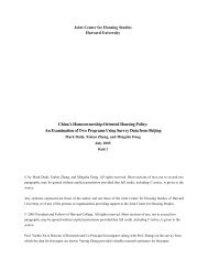
© 2001 by Ingrid Gould Ellen, Assistant Professor, New York University, Wagner School of Public Service;
Scott Susin, Research Fellow, U.S. Bureau of the Census; Amy Ellen Schwartz, Associate Professor of Public
Administration, Wagner School of Public Service; Michael H. Schill, Professor of Law and Urban Planning,
New York University School of Law; Robert F. Wagner, Graduate School of Public Service. All rights
reserved. Short sections of text, not to exceed two paragraphs, may be quoted without explicit permission
provided that full credit, including copyright notice, is given to the source.
The research upon which this paper is based was funded by the Fannie Mae Foundation. All of the views
expressed, however, are those of the authors, alone. The authors would like to thank Ioan Voicu for excellent
research assistance and Frank DeGiovanni, Denise DiPasquale, Fran Justa , Bruce Katz, Susan Wachter, and
participants at the Joint Center for Housing Studies Symposium on Low-Income Homeownership for their
insightful comments. They would also like to express their gratitude to Jerilyn Perine, Richard Roberts,
Harold Shultz, and Calvin Parker of the New York City Department of Housing Preservation and
Development and Sal D’Avola of the New York City Housing Partnership for providing them with the data
necessary to complete this research.
This paper was prepared for the Joint Center for Housing Studies’ Symposium on Low-Income
Homeownership as an Asset-Building Strategy and an earlier version was presented at the symposium held
November 14-15, 2000, at Harvard University. The Symposium was funded by the Ford Foundation, Freddie
Mac, and the Research Institute for Housing America.
This paper, along with others prepared for the Symposium, will be published as a forthcoming book by the
Brookings Institution and its Center for Urban and Metropolitan Policy.
All opinions expressed are those of the authors and not those of the Joint Center for Housing Studies, Harvard
University, the Ford Foundation, Freddie Mac, and the Research Institute for Housing America.

Abstract
In this paper, we look at the impact of two New York City homeownership programs on
surrounding property values. Both of these programs—the Nehemiah Plan and the New
Homes Program of the New York City Housing Partnership—develop affordable, owneroccupied
homes in distressed urban neighborhoods.
Our analysis uses a hedonic model to compare the sales prices of properties in small rings
surrounding homeownership sites to the prices of comparable properties in the same
community districts, but outside the rings. We then compare the magnitude of this
difference before and after the completion of homeownership units. Based on an analysis of
300,000 property sales, we find that prices of homes near to homeownership sites rose
significantly relative to prices in their community districts between 1974 and 1999. Part of
this increase appears associated with the construction of city-sponsored, affordable
homeownership units.

Table of Contents
I. Introduction 1
Spill Over Effects of Homeownership and Housing Redevelopment 1
New York City Housing Programs 4
Choosing Locations 5
II. Methodology 6
III. Summary of Data 10
IV. Results 18
V. Conclusion 25
References 27
Appendix A 29
Appendix B 32

I. Introduction
Promoting homeownership has always been a central aim of housing policy in the United
States. The federal tax code delivers generous tax benefits to homeowners, the Federal
Housing Administration (FHA) provides insurance on high loan-to-value mortgages, a
variety of other FHA programs have offered below-market interest rates, and the
Community Reinvestment Act of 1977 provides incentives for financial institutions to
make mortgage loans in low- and moderate-income communities. As cities have become
more centrally involved in implementing housing policy, local officials have also begun
to sponsor a large number of homeownership programs in distressed communities, such
as homeownership counseling, outreach, and efforts to subsidize production.
Although these efforts typically do not reach the poorest households, they are
justified in large part by the positive spillovers that many argue will result from the
development of new homes and from homeownership itself. 1 To date, there is little
empirical evidence about the impact of homeownership efforts on local communities. In
this paper, we investigate the impact of two of New York City’s major homeownership
programs on property values in surrounding communities. Both of these programs, the
Nehemiah Plan and the New Homes Program of the New York City Housing Partnership,
subsidize the development of affordable, owner-occupied homes in distressed urban
neighborhoods.
Spillover Effects of Homeownership and Housing Redevelopment
There are several reasons that the Nehemiah and Partnership New Homes programs
might be expected to raise the value of surrounding properties. First, both programs
replace blighted or vacant properties with new homes. Unlike most commodities, housing
is fixed in space, and the value of a home is therefore influenced not only by its structural
features and quality but also by its surroundings. The appearance of neighboring homes,
the level of noise and disorder in a community, and the quality of local public services
should all contribute to the value of a particular home. Thus, housing investments in
blighted areas should theoretically generate spillover benefits for the local community,
benefits that should be capitalized into the value of surrounding properties.
Second, beyond adding new structures where there was previously blight, these
1 Some cities may also support homeownership programs as an attempt to retain the middle-class.
1

two New York housing programs also bolstered the number of homeowners in their
communities, which may, in itself, lead to higher property values if their greater financial
stake leads homeowners to take better care of their homes than renters. Similarly, there is
some evidence that homeowners are more involved in local organizations and activities
(both because of their financial stake and because homeowners simply tend to remain in
their homes for a longer period of time); this factor may improve the quality of life in a
community and thereby raise property values (DiPasquale and Glaeser 1999; Rohe, Van
Zandt, and McCarthy 2000).
Finally, these two programs also lead to an increase in the population of their
neighborhoods, which may, in turn, have invited new commercial activity, a greater sense
of safety, and general economic growth.
There are, to date, few reliable studies examining the impact of privately
sponsored new construction on surrounding property values, largely due to the difficulty
of addressing endogeneity problems. (Private developers aim to develop sites where they
believe property values are likely to appreciate, and thus new construction itself depends
on property values.) Simons, Quercia, and Maric (1998) use cross-sectional data for
Cleveland to examine the effect of one- to three-family home construction on the sales
prices of nearby housing. They find that the existence of a newly constructed unit nearby
has a small, but positive effect on sales price. Although the authors attempt to treat
construction as endogenous using two-stage least squares, the poor performance of the
first-stage model (explaining new construction in a census tract) leads them ultimately to
use actual levels of new construction in their regression models.
Most studies of the relationship between investments in housing and
neighborhood property values focus instead on the impact of proximity to publiclysubsidized
housing, and in particular, proximity to federally-subsidized rental programs.
So far, few studies suggest much of an effect. Nourse (1963) and Rabiega, Lin, and
Robinson (1984), for example, examine the effect of newly developed public housing on
neighboring property values and both find modest, positive impacts, but only in limited
cases. More recently, Chandler, Benson and Klein (1993) find that the siting of scatteredsite
public housing in Cleveland was associated with increases in sales prices in 8 of 12
census tracts, but these authors do not control for the effects of neighborhood conditions.
In a more thorough analysis, Briggs, Darden, and Aidala (1999) undertake a pre/post
2

analysis of home sales in the vicinity of seven scattered-site public housing developments
in Yonkers, New York, and report no impact on sales prices.
Several recent and careful studies find that proximity to subsidized rental housing
may in fact depress property values. Lyons and Loveridge (1993), Goetz, Lam, and
Heitlinger (1996), and Lee, Culhane, and Wachter (1999) all find small statistically
significant negative effects on housing value associated with the presence of subsidized
housing in a neighborhood.
In short, there is no consensus about the effects of subsidized housing on
surrounding property values. Moreover, in all of these studies (as in those of private
housing), data limitations make it difficult to pinpoint the direction of causality. Are
subsidized sites systematically located in weak neighborhoods or do subsidized sites lead
to neighborhood decline? Most of these prior studies utilize cross-sectional data and thus
cannot determine whether neighborhoods with subsidized housing are systematically
different from those without. 2 One recent study utilizes a research design that far more
persuasively sorts out causality to study the impact of neighbors who use Section 8
certificates and vouchers (Galster, Tatian, and Smith 1999). We borrow from their
methodology, adapting it to study the development of new owner-occupied homes.
Virtually all of these earlier studies focus on rental housing; only two examine the
impact of publicly assisted homeownership programs. Lee, Culhane, and Wachter (1999)
find that FHA-insured units and units developed through the Philadelphia Housing
Authority’s homeownership program both seem to have positive impacts on surrounding
house prices. This is precisely the opposite of the study’s conclusions concerning rental
housing (discussed above)—the Section 8 New Construction Program is the only rental
housing program that appears to have a positive effect on property values. Although these
results seem to suggest that homeownership and new construction have uniquely positive
effects on surrounding property values, a more recent study raises doubts. In their study
of Nehemiah housing developments in Philadelphia, Cummings, DiPasquale, and Kahn
(2000) find no evidence of spillover effects of these new owner-occupied homes on
surrounding property values. 3
2 Briggs, Darden, and Aidala (1999) utilize longitudinal data but they do not control for before and after
price trends in the neighborhoods surrounding the public housing sites.
3 As discussed above, many argue that an increase in the proportion of homeowners should in itself bolster
3

New York City Housing Programs
In 1986, New York City launched an unprecedented initiative to rebuild its housing stock
that was devastated in the 1970s. Since then, the city’s housing agency has invested close
to $five billion in the construction of over 22,000 homes, the gut rehabilitation of more
than 43,000 units of formerly vacant housing, and the moderate rehabilitation of over
97,000 units of occupied housing. 4 Most of these efforts have focused on low- and
moderate-income rental housing, but a few programs sponsor ownership housing.
The Nehemiah Program
The Nehemiah Program was launched in the early 1980s by East Brooklyn Churches, a
group of 36 churches in Brooklyn. The first house was completed in 1984; in total, nearly
3,000 homes have been built through the program. About 80 percent of these homes have
been built in Brooklyn, with the remaining homes built in the South Bronx by another
group of churches (Stuart 1997). The Nehemiah program has typically built projects of
500 to 1,000 units each on large tracts of donated city-owned land. The units are very
modest, 18-foot-wide homes, built in identical, block-long rows of single-family homes.
The high-volume, mass-production approach has allowed the Nehemiah program
to deliver units at a very low cost. The Brooklyn units cost about $60,000 to build and
sold for approximately $50,000, as a result of a $10,000 city subsidy that must be repaid
upon resale (Orlebeke 1997). For the later units built in the South Bronx, the typical cost
of a unit was approximately $71,000, and the purchase price was lowered to $56,000
through a non-interest bearing, $15,000 second mortgage from the city, due only upon
resale (Donovan 1994).
The Partnership New Homes Program
The New York City Housing Partnership is a not-for-profit intermediary that was
organized in 1982 to help create and manage an affordable homeownership production
program in the city (Wylde 1999). Its core program—the New Homes Program—was
property values. Is the value of a property higher (or does it appreciate more rapidly) when it is located in a
community with a greater share of homeowners? Few studies tackle this question, again perhaps because of
concerns about endogeneity. But in an analysis of 2,600, non-affluent urban census tracts between 1980
and 1990, Rohe and Stewart (1996) suggest the answer is yes. Their results imply that for each percentage
point increase in a census tract’s 1980 homeownership rate, the value of its typical single-family home
increased by roughly $1,600 more between 1980 and 1990.
4 Estimates of activity beginning in fiscal year 1987 and ending in fiscal year 1998.
4

launched soon after. Like the Nehemiah Program, the New Homes Program also
developed new, affordable, owner-occupied homes in distressed communities. Typically,
these homes are built by private, profit-motivated developers selected by the city and the
Housing Partnership. But unlike Nehemiah, the Partnership has not typically built on
large contiguous lots. More than three-quarters of the Partnership projects are less than
100 units, many of them packages of small, infill sites grouped together to make up a
project (Orlebeke 1997). What is more, the Partnership has typically developed two- and
three-family homes that include an owner’s unit plus one or two rental units.
In part because of this different approach to design and construction, the
Partnership projects have tended to be more costly. According to one 1988 study of 10
Partnership projects, per-unit costs during the 1980s ranged from $57,000 to $137,000
(Orlebeke 1997). The projects were sold in turn to slightly higher income households
than the Nehemiah Program homes. In all Partnership projects, the city has provided the
land at a nominal cost ($500 per lot) and has given a $10,000 subsidy per home; the State
Affordable Housing Corporation has provided an additional $15,000 per home (Donovan
1994).
By June of 1999, the Partnership New Homes program had added 12,590 new
homes to New York City’s boroughs. Like the Nehemiah Program, the construction has
been concentrated in Brooklyn and the Bronx, but roughly one-quarter of the homes have
been built in New York’s other three boroughs.
Choosing Locations
In testing the impact of new housing on surrounding areas, there is always some concern
about site selection. In this case, for instance, the city may have aimed to select “strong”
sites for these programs, where they believed property values were beginning to increase
(or at least had some hope of doing so). However, even if the city had wanted to choose
promising sites, there were considerable constraints in doing so. First, the site had to be
owned by the city, which meant it would have had to be abandoned by its previous owner
and vested in an in rem proceeding for delinquent property taxes. The city’s stock of
abandoned properties was overwhelmingly concentrated in its poorest neighborhoods
(Scafidi, Schill, Wachter, and Culhane 1998). Second, in the case of the Nehemiah
Program, the land had to be a large, mostly vacant, contiguous parcel of land.
In any case, interviews with city officials suggest that the city did not give its best
5

vacant sites to the Partnership and Nehemiah sponsors. In many instances, the city was
also interested in realizing a high return from its land holdings. As Anthony Gliedman, a
former Commissioner of New York City’s Department of Housing Preservation and
Development put it, “Why would we do market rate sites with the Partnership?”
(Orlebeke 1997). In other words, the process of selecting individual sites, while perhaps
not fully random, was certainly far from one that sought to systematically pick winners.
Nonetheless, our research design (as outlined below) should help to control for
systematic selection issues.
II. Methodology
The centerpiece of this research utilizes a hedonic price function. In hedonic price
analysis, housing is viewed as a composite good or a bundle of services. Observed house
prices are the product of the quantity of housing services attached to the property and the
price of these housing services, summed over all structural and locational characteristics
of the property. The basic model takes the following form:
P it = α + βX it + γZ it + δI+ є it
where P it is the sales price of property i at time t, X is a vector of property-related
characteristics, including age and structural characteristics, Z is a vector of locational
attributes, such as local public services and neighborhood conditions, and I isavectorof
dummy variables indicating the year of the sale. The derivative of the housing price
function with respect to an individual attribute may then be interpreted as the implicit
price of that attribute (Rosen 1974). In many cases, housing prices are entered as logs (as
we do below), so the coefficients are then interpreted as the percentage change in price
that results from an additional unit of the independent variable.
As suggested above, the price of housing is affected by a broad array of structural
and neighborhood characteristics and estimating equation (1) therefore requires a great
deal of detailed data. Unfortunately, if some relevant variables cannot be included, either
because they are unmeasured or because data are unavailable, the coefficients on the
included variables may be biased. Thus, in trying to identify the independent effect of
proximity to Partnership and Nehemiah homes, our challenge is to control for a sufficient
number of neighborhood attributes so that our results do not suffer from omitted variable
bias.
6

Our basic approach is to compare prices of properties in the micro-neighborhoods
(or rings) surrounding Nehemiah and Partnership sites to prices of comparable properties
that are outside the ring, but still located in the same general neighborhood. Then we
examine whether this magnitude of this difference has changed over time, and if so, if the
change is associated with the completion of a Partnership or Nehemiah project. This
approach weeds out any systematic differences between the general neighborhoods
chosen for these homeownership projects and other locations around the city, differences
that have little to do with the impact of the actual projects and that could otherwise
confound our results. Thus, our approach should yield an unbiased measure of impact, as
long as we have sufficient data on the structural characteristics of the homes that sell and
as long as there are few other neighborhood influences that shape the value of properties
very near to the Partnership and Nehemiah sites around the time of project completion
but that do not also color property values in the general neighborhood.
More specifically, we estimate the following specifications:
(2) LnP = a + bX + cCD*Year + dRing500*Years from sale + є
(3) LnP = a + bX + cCD*Year + dRing1000*Years from sale + є
(4) LnP = a + bX + cCD*Year + dRing2000*Years from sale + є
where X is a vector of structural characteristics and CD*Year is a vector of year-specific
neighborhood dummy variables indicating the year of sale and the neighborhood in which
the property is located (measured by community district). These CD*Year dummy
variables control for community-specific trends in prices. New York City is divided into
59 community districts, each of which has an average population of 125,000 residents.
Although a smaller geographic area may be more appealing as a proxy for a
neighborhood, these 59 community districts serve as the city’s main administrative units
for services and other amenities and are widely recognized by residents as distinct
neighborhoods and housing markets. 5
In addition to these CD*Year fixed effects, we control for differences in both
price levels and trends for properties near to Nehemiah and Partnership sites by using a
set of 20 dummy variables that indicate whether a sale is within a given distance of a
5 The high density of New York City makes using census tracts undesirable. In many instances, the 2,000-
foot rings around developments included multiple census tracts and that would have significantly
complicated the interpretation of the results.
7

project site and the number of years it is prior to or after project completion. 6 The first
model, for instance, includes a dummy variable indicating if the property sold is located
within 500 feet of a future Nehemiah or Partnership site and sold 10 years prior to project
completion, another indicating if it is within 500 feet and sold nine years prior to project
completion, and so on. Similarly, the model includes a dummy variable noting if the
property is located within 500 feet of a Nehemiah or Partnership site and sold within one
year after completion, another indicating if it is within 500 feet and sold between one and
two years after completion, and so on. The second model includes the analogous 20
dummy variables that correspond to the ring of properties within 1,000 feet of a
homeownership site.
The coefficients on these dummy variables can be interpreted as the percentage
difference between the prices of properties in the rings surrounding the homeownership
project and the prices of properties that are outside that ring but inside the community
district. We track how the gap between the ring and the community district was changing
prior to the completion of the homeownership project, how it changed after project
completion, and whether there was any discontinuous shift in the magnitude of the gap
after completion.
It is important to stress that it is not clear what single measure of project impact is
most appropriate. A simple comparison of the gap one year prior to project completion
and the magnitude of the gap one year after completion is likely to be inadequate because
it may take a while for the full impact of the project to be felt. Moreover, it is also
possible that, once a project is announced or started, property values may begin to rise in
anticipation of the effect the project will have on the surrounding community. (According
to HPD staff, community residents were involved in the planning process and often knew
about these projects years before the start of construction.) If so, then prices would
already be rising prior to completion and using one year prior to completion as a
benchmark is conservative.
Another issue is that the gap between home prices in the rings and the larger
community districts might have been shrinking (or expanding) even before the advent of
these projects, in which case a simple pre/post comparison will overstate (or understate)
6 In cases where a sale was within 500 feet of more than one Nehemiah or Partnership project, we use the
date for completion of the first project.
8

the magnitude of the impact. While the methodology above allows us to see these preand
post-completion trends, it does not provide an easy way to measure the degree to
which the change in the gap after development exceeded what would have occurred,
given prior trends. To arrive at a summary measure of impact that controls for these prior
trends (that is, a summary measure that controls for how the gap between prices in the
rings and prices in their community districts has been changing over time), we use a
methodology similar to Galster, Tatian, and Smith (1999) and estimate the following
three equations: 7
(5) LnP = a + bX + cCD*Year + dRing500 + ePostring500 + fspline(T500) +
gTPost500 + є
(6) LnP = a + bX + cCD*Year + dRing1000 + ePostring1000 + fspline(T1000) +
gTPost1000 + є
(7) LnP = a + bX + cCD*Year + dRing2000 + ePostring2000 + fspline(T2000)
+gTPost2000 + є
where X is a vector of structural characteristics, such as building age or size, and
CD*Year is again a vector of year-specific neighborhood dummy variables indicating the
year of sale and the community district in which the property is located. We then include
a set of variables that capture whether a sale is within a given distance of a project site.
The first model, for instance, includes Ring500, a dummy variable indicating if the
property is located within 500 feet of a Nehemiah or Partnership site regardless of
whether development has been completed. The second model includes Ring1000,
indicating if the property is located within 1,000 feet of one of the sites, and the third
model includes Ring2000, which indicates if the property is located within 2,000 feet of
one of the sites.
Each model also includes a variable to measure whether a sale takes place after a
project is completed. PostRing500 is a dummy variable that equals 1 if the property sale
occurs within 500 feet of a completed Nehemiah or Partnership development. Similarly,
7 The key difference with Galster, Tatian, and Smith (1999) is that we include CD*Year fixed effects that
allow for community district-specific trends in prices. They use tract-fixed effects instead, which use a finer
level of geography but assume that neighborhood-fixed effects are constant over time. As mentioned above,
the high density of New York City makes using census tract*year-fixed effects impractical. Another
difference is that we use splines for the time trends to capture a non-linear pattern.
9

PostRing1000 and PostRing2000 are dummy variables indicating if the sale occurs within
1,000 or 2,000 feet, respectively of a completed project. The coefficients on these
PostRing variables are critical. They indicate the extent to which, after the completion of
a homeownership development, sales prices rise in the vicinity, relative to the average
increase in the larger community district.
T500, T1000, and T2000 are time trends, specific to each of the three rings. The
time trends are equal to “1” in 1975, “2” in 1976 and so on. They are modeled as fivesegment
linear splines, which allows them to capture a much more flexible pattern than a
simple linear trend. These time splines help to mitigate concerns about selection bias (ie.
the possibility that the city sought to place projects in locations where prices were going
to increase even without city investment) by controlling for overall trends in housing
prices in these micro-neighborhoods surrounding the development. The danger of
including the trends, however, is that they may also pick up some of the effects of the
developments themselves, since, as explained above, property values may begin to rise
once a project is announced or started, in anticipation of the effect the project will have
on the surrounding community. If so, then including these splines means that we simply
measure the added effect that a project’s completion has on property values, above and
beyond the effect of its announcement or start, and that we understate the full impact.
TPost500, TPost1000, and TPost2000 are post-occupancy trend variables for the
500, 1,000, and 2,000 feet rings respectively. TPost500, for instance, equals 1 if sale is
located within 500 feet of a site and occurs within the first year after the project is
completed. If prices appreciate more rapidly in the rings after a project is completed, then
these coefficients will be positive.
III. Summary of Data
To undertake the analysis outlined above, we have obtained detailed data from a number
of unique city data sources. First, through an arrangement with the New York City
Department of Finance, we obtained a confidential database containing sales transaction
prices for all apartment buildings, condominium apartments, and single-family homes
from 1975 to 1998. 8 Limiting the analysis to properties that are located within the 34
8 Because sales of cooperative apartments are not considered to be sales of real property, they are not
recorded and are thus not included in this analysis. This is unlikely to have a major impact on our results
10

community districts where Nehemiah or Partnership New Homes projects were
developed, our sample includes 300,890 sales. 9 Because of the long time span of the data
and New York City’s size, the sample size is large compared too much of the literature.
Second, we have supplemented these transactions data with building characteristics
from an administrative data set gathered for the purpose of assessing property taxes (the
RPAD file). The RPAD data contain information about buildings and do not contain
much information about the characteristics of individual units in apartment buildings
(except in the case of condominiums). 10 Nonetheless, these building characteristics
explain variations in prices surprisingly well (perhaps because over 70 percent of
buildings are either single-family or two-family homes). Using all transactions in 1998, a
regression of the log price per unit on building age and its square, log square feet per unit,
the number of buildings on a lot, and dummies for the presence of a garage,
abandonment, major alterations, the presence of commercial units, and location on a
block corner yields an R 2 of 0.46. When a set of 18 building classifications is added to
the regression (for example, “single-family detached,” “single-family attached,” “twofamily
home”), the R 2 rises to 0.68. Finally, when community district dummy variables
are added as well, the R 2 rises to 0.78.
Figure 1 shows summary statistics from the RPAD data. The first column shows
characteristics of our full sample; the second shows the characteristics of sales located
within 500 feet of a Nehemiah or Partnership site, whether completed or not. As shown,
nearly three-quarters of all buildings sold were either one- or two-family homes, and over
92 percent were either one-family homes, two-family homes, or small apartments. Most
sales were located in Brooklyn and Queens, both because of the location of the
because cooperative apartments tend to be under-represented in the 34 community districts which have
Nehemiah or Partnership New Homes developments.
9 This includes three community districts in Manhattan, nine in the Bronx, 12 in Brooklyn, nine in Queens,
and one in Staten Island.
10 It is important to note that most of the RPAD data in this study were collected in 1999; it is conceivable
that some building characteristics changed between the time of sale and 1999. However, most of the
characteristics used in the hedonic regressions are fairly immutable (e.g., corner location, square feet,
presence of garage). Furthermore, to examine whether the building characteristics tend to remain constant
over time, we merged RPAD data from 1990 and 1999 and found that for eight of the 10 variables, the
characteristic remained unchanged in 97 percent or more of the cases. “Year Built” and “Number of Units”
remained unchanged in only 87 and 93 percent of the cases respectively. We suspect that the majority of
these changes are corrections, rather than true changes, since these characteristics may change very rarely.
Thus, the 1999 RPAD file may actually be a better estimate of 1990 characteristics than the 1990 file. The
abandonment variable was collected in 1980.
11

Figure 1: Characteristics of Properties Sold
(Universe=all sales in community districts with at least one Nehemiah or partnership unit)
Percentage of All Property
Sales
Percentage of Sales Within
500 Feet of Nehemiah or
Partnership Site
Borough
Manhattan 1.3 3.1
Bronx 6.8 19.2
Brooklyn 37.3 43.1
Queens 47.0 30.5
Staten Island 7.5 4.1
Building Class
Single-family detached 25.3 15.2
Single-family attached 13.2 6.6
Two-family 34.8 36.2
Walk-up apartments 19.1 28.6
Elevator apartments 0.8 0.6
Loft buildings 0.0 0.0
Condominiums 2.9 7.1
Mixed-use (includes store or office
plus residential units) 3.8 5.6
Built pre-war 80.0 90.8
Vandalized 0.0 0.2
Other abandoned 0.2 0.6
Garage 37.0 17.1
Corner location 7.9 7.7
Major alteration prior to sale 1.7 2.9
Within 500 ft of homeownership project 4.4 100
Within 1000 ft of homeownership project 10.6 100
Within 2000 ft of homeownership project 24.5 100
300,890 13,162
12

community districts with Nehemiah or Partnership developments and because those
boroughs include a large share of smaller properties which sell more frequently than
apartment buildings (more common in Manhattan and the Bronx). The figure also shows
that over a third of the transacting properties had garages and 80 percent were built
before World War II. Only a handful of buildings were vandalized or otherwise
abandoned. Finally, the figure also shows that 4.1 percent of the properties in our sample
are located within 500 feet of a Partnership or Nehemiah site (whether completed or not),
10.6 percent are located within 1,000 feet, and 24.5 percent are located within 2,000 feet
of one of the homeownership developments.
The second column reveals some systematic differences between properties located
close to Nehemiah or Partnership sites and those that are not. Due to the location and
concentration of Partnership and Nehemiah developments, properties located within the
500-foot ring are much more likely to be in Brooklyn, Manhattan, or the Bronx.
Properties in the ring are also much older, much less likely to be single-family homes,
more likely to be walk-up apartments, and consistent with these differences, much less
likely to have garages.
Third, the New York City Department of Housing Preservation and Development has
provided us with data on the precise location (down to the block level) of all housing
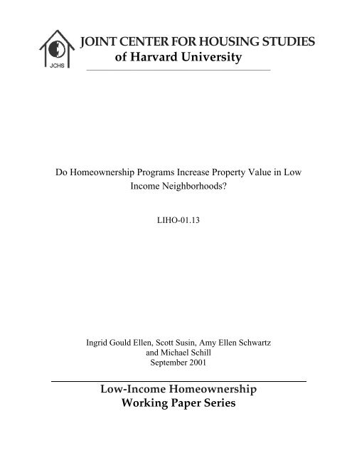
built through the Nehemiah and Partnership programs. Figure 2 shows the location of
these projects in the city. As shown, most of the projects have been built in Brooklyn and
the Bronx. Figure 3 indicates that 12,468 of the 15,528 units (80 percent) are in Brooklyn
or the Bronx and that over 13,000 (85 percent) were completed during the 1990s. As for
building type, 90 percent of the Nehemiah units are single-family homes, as compared to
just 12 percent of the Partnership units. Partnership units are instead more typically twoand
three-family homes.
Figure 4 compares the average 1990 characteristics of census tracts that include
Nehemiah and Partnership units in 1998 to those that do not. 11 The 2,938 Nehemiah units
have been built across 25 census tracts in the city (118 units per tract on average). The
Partnership units have been more dispersed, with each of the Partnership census tracts
housing an average 70 Partnership homes.
11 The census tract data is taken from the 1990 Census. Tracts are characterized as including Nehemiah or
Partnership projects, even if these projects were not built until later in the decade.
13

Figure 2: Characteristics of Units Built Through Nehemiah
and Partnership New Homes
Nehemiah Partnership New Homes Total
Borough
Bronx 544 5,426 5,970
Manhattan 0 948 948
Brooklyn 2,394 4,104 6,498
Queens 0 1,226 1,226
Staten Island 0 886 886
Building Type
One-family 2,632 1,572 4,204
Two-family 18 7,020 7,038
Three-family 0 1,659 1,659
Condominium 288 2,112 2,300
Cooperative 0 227 227
Year Completed
1984 194 0 194
1985 170 18 188
1986 235 232 467
1987 284 263 547
1988 240 260 500
1989 317 226 543
1990 460 1,918 2,378
1991 218 867 1,134
1992 140 1,555 1,695
1993 108 1,104 1,252
1994 120 1,567 1,687
1995 138 1,183 1,321
1996 30 1,018 1,048
1997 44 1,119 1,163
1998 126 664 790
1999 114 596 710
Total 2,938 12,590 15,528
14

Figure 3:
Location of Partnership and Nehemiah Developments
Number of
Units
30
150
300
15

Figure 4: 1990 Characteristics of Census Tracts in which
Partnership and Nehemiah Projects Are Located
Percent
Tracts with
Nehemiah Units
Percent
Tracts with
Partnership Units
Mean Poverty rate 40.1 32.5 18.4
Percent of tracts with poverty rate >= 20% 96.0 71.0 33.6
Percent of tracts with poverty rate >= 40% 48.0 37.4 12.5
Percent
All Tracts in
New York
City
Mean percentage of households on public 33.0 27.3 13.8
assistance
Mean family income $24,579 $29,342 $46,665
Mean unemployment rate 18.5 14.8 9.7
Mean percentage of adult residents with some 23.4 27.0 39.7
college education
Mean percentage black 72.0 51.5 28.9
Mean percentage Hispanic 32.3 39.3 21.9
Mean homeownership rate 20.1 24.2 34.8
N 25 179 2,131
This figure also confirms that these projects were located in distressed neighborhoods
and suggests that the neighborhoods in which Nehemiah units have been located are
somewhat more disadvantaged. For example, the average poverty rate in a tract with
Nehemiah and Partnership units was 40.1 and 32.5 percent respectively, as compared to
just 18.4 percent for tracts citywide. Similarly, while just 12.5 percent of census tracts in
New York had poverty rates of at least 40 percent, 37 percent of those with Partnership
units and 48 percent of those with Nehemiah units had poverty rates this high.
The other socioeconomic variables tell the same story. Mean family income was
$24,579 in Nehemiah tracts, compared to $29,342 for Partnership tracts and $46,665 in
all tracts citywide. The unemployment rate was twice as high in census tracts with
Nehemiah units than it was in the average city neighborhood. As for racial and ethnic
composition, the Nehemiah and Partnership tracts housed a greater share of Hispanic
residents and a much larger share of Black residents than the average tract in the city.
Finally, the neighborhoods where Partnership and Nehemiah projects were located have
exceptionally low rates of homeownership. Less than one-fourth of households on
average own their homes in these communities, as compared to an average of 35 percent
16

in census tracts citywide.
As mentioned above, we used GIS techniques to measure the distance from each
sale in our database to all Nehemiah and Partnership sites. 12 Then we effectively created
rings around each project to determine whether the prices of properties in the rings
surrounding the developments were affected by their proximity to these new
homeownership developments. To give a sense of these rings, Figure 5 shows an example
of a Partnership development located on the Brooklyn/Queens border and its surrounding
rings. The innermost ring extends 500 feet (usually one to two blocks) from the project;
the second ring extends 1,000 feet (one to four blocks), and the outermost ring extends
2,000 feet (three to eight blocks).
Figure 5
Partnership Development on Brooklyn/Queens Border
Park
Cemetery
12 Since all buildings in New York City have been geocoded by the New York City Department of City
Planning, we used a “cross-walk” (the “Geosupport File”) which associates each tax lot with an x,y
coordinate (i.e., latitude, longitude, using the U.S. State Plane 1927 projection), police precinct, community
district, and census tract. A tax lot is usually a building and is an identifier available to the homes sales and
RPAD data. We are able to assign x,y coordinates and other geographic variables to over 98 percent of the
repeat sales using this method. For the Nehemiah and Partnership data, only the tax block on which the
property is located (which corresponds to a physical block) is available. After collapsing the Geosupport
file to the tax block level (i.e., calculating the center of each block), we were able to assign an x,y
coordinate to 99.7 percent of these projects.
17

The RPAD and homes sales data do not identify whether a particular property
received city subsidies. In order to insure that we analyze only the sales prices of
buildings neighboring Partnership and Nehemiah developments, and not the sales prices
of the developments themselves, we exclude any sales that could potentially be part of a
development. Specifically, we excluded 2,248 sales that occurred on the same block as a
Nehemiah or Partnership development if the sale was of a building that was constructed
after the Nehemiah or Partnership building had been completed. 13
IV. Results
As discussed above, our central empirical strategy is to test whether and how sales prices
in the rings surrounding homeownership projects change relative to prices in their
community districts, after the completion of those projects. Before presenting regression
results, it is useful to show how average prices within 500 feet of a homeownership site
compare to average prices in our sample, both before and after the completion. Figure 6
shows that during our time period, per unit sales prices for buildings located within 500
feet of a Nehemiah or Partnership site were on average 60 percent lower than the prices
of all buildings located in the 34 community districts. These projects, in other words,
have clearly been located in neighborhoods with depressed housing prices. 14 Again, given
that these projects were developed on vacant city-owned land that the city was willing to
provide at nominal prices, it is not surprising that prices are relatively low in the
surrounding area.
Yet, the figure also shows that one year after the completion of the actual projects, per
unit sales prices for buildings located within 500 feet of a Nehemiah or Partnership site
were on average only 28 percent lower than prices of all buildings in the 34 community
districts. One year after the completion of the average Nehemiah or Partnership project,
13 To provide a margin of error with respect to the recording of construction dates in RPAD, we also
excluded sales of buildings on the same block as a Partnership and Nehemiah development that were built
up to five years before the Partnership or Nehemiah building. These exclusions are included in the total
2,248 figure.
14 Given the evidence shown in Figure 5 that the census tracts surrounding Nehemiah and Partnership sites
are notably less affluent than the city at large, it is no doubt true that prices in the rings surrounding these
sites are even lower in comparison to average prices in all community districts.
18

that is, the differential between property values in the 500-foot ring and property values
for all buildings shrunk by 32 percentage points. Property values were still below those
overall, but the differential appears to shrink considerably after the construction of these
homeownership projects. As shown, the differential between property values in the ring
and those in the 34 community districts actually rises in year 3, but still remains 23
percentage points lower than it was prior to the completion of a development.
Figure 6: Differences in Differences
Percentage Difference Between Price in 500-Foot Ring and Average Annual Price,
by Time from Development
Ring Price
Relative to
Average Price
Diff-in-Diff
(Relative to Diff
Before
Completion)
Standard Error
(Dff-in-Dff)
Before completion
of development -0.605
After completion
1 year -0.290 0.315 0.026 12.3
2 years -0.293 0.312 0.027 11.6
3 years -0.366 0.239 0.028 8.7
4years -0.337 0.269 0.025 10.6
5 years -0.354 0.251 0.029 8.5
T-statistic
(Diff-in-Diff)
The real question, of course, is whether this same story persists after we control
for property characteristics and changes in local neighborhoods. To isolate the influence
of proximity to a completed homeownership project, we estimate the regressions
discussed above, in which the dependent variable is the log of the sales price per unit, and
which control for building and local neighborhood characteristics and include a full
complement of community district and year interaction effects (CD*Year fixed effects). 15
This controls for a community district-specific trend in housing prices and thus allows us
to test whether any shift in housing prices (either level or trend) that occurs after the
homeownership properties are constructed is distinct from the pattern of prices in the
surrounding community district.
15 We effectively include 25 dummy variables (a different dummy for each year from 1975–1999) for each
of the 34 community districts in the sample, for a total of 850 dummy variables.
19

Figure 7: Selected Coefficients from Regression Results with Year*
Ring Dummy Variables
Dependent Variable = Log of Price Per Unit
Model 1 Model 2 Model 3
(500-ft. Ring) (1000-ft. Ring) (2000-ft. Ring)
>=10yr_pre_ring -0.2265 -0.2004 -0.1660
(0.0056) (0.0037) (0.0027)
9yr_pre_ring -0.2463 -0.2086 -0.1770
(0.0143) (0.0095) (0.0065)
8yr_pre_ring -0.2350 -0.2095 -0.1721
(0.0150) (0.0095) (0.0064)
7yr_pre_ring -0.1293 -0.1663 -0.1670
(0.0146) (0.0093) (0.0063)
6yr_pre_ring -0.1693 -0.1726 -0.1661
(0.0145) (0.0094) (0.0063)
5yr_pre_ring -0.1360 -0.1544 -0.1554
(0.0143) (0.0093) (0.0063)
4yr_pre_ring -0.1433 -0.1283 -0.1384
(0.0147) (0.0097) (0.0064)
3yr_pre_ring -0.1142 -0.1280 -0.1472
(0.0154) (0.0099) (0.0068)
2yr_pre_ring -0.0864 -0.1086 -0.1117
(0.0145) (0.0095) (0.0067)
1yr_pre_ring -0.1036 -0.1046 -0.1164
(0.0134) (0.0091) (0.0065)
1yr_post_ring -0.0374 -0.0921 -0.0903
(0.0130) (0.0091) (0.0067)
2yr_post_ring -0.0299 -0.0497 -0.0845
(0.0152) (0.0101) (0.0069)
3yr_post_ring -0.0529 -0.0454 -0.0610
(0.0162) (0.0103) (0.0073)
4yr_post_ring -0.0289 -0.0487 -0.0665
(0.0150) (0.0107) (0.0074)
5yr_post_ring -0.0436 -0.0824 -0.0863
(0.0167) (0.0110) (0.0076)
6yr_post_ring -0.0609 -0.0949 -0.0868
(0.0191) (0.0120) (0.0080)
7yr_post_ring -0.0514 -0.0809 -0.0829
(0.0200) (0.0124) (0.0081)
8yr_post_ring -0.0999 -0.1032 -0.0771
(0.0229) (0.0137) (0.0089)
9yr_post_ring -0.0389 -0.0723 -0.0733
(0.0255) (0.0163) (0.0101)
>=10yr_post_ring -0.0837 -0.0752 -0.0559
(0.0208) (0.0115) (0.0070)
Adjusted R 2 0.801 0.802 0.804
N 300,890 300,890 300,890
Note: Standard errors in parentheses. See Appendix A for full results.
20

The estimated coefficients for the ring variables and their standard errors are
shown in Figure 7. The complete model specification with the coefficients for the
structural variables is included in Appendix A. These structural variables have the
expected signs. 16 The per unit sales price is higher if a building is larger or newer, located
on a corner, or includes a garage. The price is lower if the building is vandalized or
abandoned. The building class dummies are also consistent with expectations. Sales
prices for most of the building types are lower than those for single-family attached
homes (the omitted category). One result, perhaps counter-intuitive, is that the estimated
impact of the dummy variable indicating that the building has undergone a major
alteration prior to sale is statistically insignificant. This result may reflect the fact that
buildings that have undergone such major alterations are generally in worse shape and
lower-priced prior to renovation in ways that are not captured by our data. 17
The key coefficients, those on the ring dummy variables, are presented in Figure
7. Again, each of these coefficients may be interpreted as the percentage difference
between the price of properties within the rings and comparable properties located
outside the rings but within the same community district. (The coefficient on Ring500,
one year before completion, for instance suggests that properties located within 500 feet
of a future Partnership or Nehemiah project one year prior to completion sold for 10.4
percent less than comparable properties beyond 500 feet but in the same community
district.)
The first point to note is that all the coefficients are negative and virtually all are
statistically significant. Consistent with the uncontrolled results set forth in Figure 6, that
is, prices of properties located in the rings are significantly lower than the prices of
comparable properties located in their community district, both before and after project
completion. The second point to note is that the coefficients generally get smaller over
time. Prices in the rings, that is, rise over time relative to prices in the larger community
16 The odd-shape and extension variable are included to capture any irregularities in the calculation of
square footage.
17 It is worth mentioning the statistically significant coefficients on the dummy variables indicating if the
age or size of a building is missing. In general, these suggest that the buildings for which age is missing are
older than others and the buildings for which square footage is missing are larger. The condominiums for
which square footage is missing (90 percent of sales missing square feet) are also larger, but somewhat less
so. In total, just over one percent of property sales did not indicate square footage and three percent did not
indicate age.
21

district both before and after completion. However, there does appear to be a significant
reduction in the gap around the time of completion. Finally, it is interesting to note that,
while the gap between prices in the ring and the community district falls immediately
after completion in the 500-foot ring, it appears to take longer for the effects to be felt in
the more distant rings. The major decline in the 1,000-foot ring occurs between one and
two years after the completion of the homeownership project. In the 2,000-foot ring, the
decline continues through year three. One plausible explanation is that the
homeownership projects have a more sudden impact on their immediate surroundings,
but that, over time, they may bring benefits to more distant areas as well. (This is also
consistent with the fact—discussed below—that after 10 years the impact in the 500-foot
ring appears to dissipate—while the effects are persistent in the 2,000-foot ring.)
Figure 8
Percent Difference Between Prices in 500 Foot Ring and Community
District, by Time to Completion
0
-10 -5 0 5 10 15
Percent Difference Between Ring and CD
-5
-10
-15
-20
-25
-30
Time to Completion (0= 1 year before)
Figure 8 graphs these percentage differentials by the year relative to project
completion and clearly shows that the gap has declined over time. One year before the
completion of a homeownership project (marked by zero on the graph), the sales price of
a building within 500 feet of a future site is on average 10.4 percent lower than the price
of a comparable home sold in the same year in the same community district. In the years
22

after completion, the gap shrinks by an average of 5.6 percentage points to only 4.8
percent lower than the price of a comparable property in the community district.
As this picture also shows, however, the average price differential between the
rings and their community districts was already declining prior to project completion.
Even without the homeownership development, perhaps, it might have continued to
decline. On the other hand, some of the decline that occurred prior to project completion
might in fact have been due to the construction or announcement of the new owneroccupied
homes.
Figure 9: Selected Coefficients from Regression Results with Ring-Specific, Time-Trend
Dependent Variable = Log of Price Per Unit
Model 1 Model 2 Model 3
Ring500 -0.195
(0.019)
Ring1000 -0.158
(0.012)
Ring2000 -0.125
(0.009)
PostRing500 0.039
(0.012)
PostRing1000 0.019
(0.008)
PostRing2000 0.017
(0.005)
TPost500 -0.008
(0.002)
TPost1000 -0.005
(0.001)
TPost2000 -0.001
(0.001)
Adjusted R-squared 0.801 0.802 0.804
N 300,890 300,890 300,890
Note: All regressions include ring-specific time trends, modeled as a five-segment linear spline. See
Appendix B for full results, including time spline. Standard errors in parentheses.
Thus, as mentioned above, this specification does not provide a clear summary
measure of impact. To arrive at such a measure, we estimate an alternative specification
that offers an estimate of impact above and beyond what would have been predicted
given prior trends in prices in the ring. To control for these trends, these specifications
model time for the ring properties as a linear spline with five segments (see equations 5
23

through 7 above). Figure 9 summarizes these coefficients, and the full set of coefficients,
including the time spline, may be found in Appendix B. Consistent with the results
above, the coefficients on the first set of ring dummies (Ring500, Ring1000, Ring2000)
indicate that prices in the rings surrounding these properties are significantly lower than
prices elsewhere in the city—or more precisely, they are lower than the prices of
comparable properties elsewhere in their community district. (These dummy variables
indicate whether or not a property is located within a certain distance of one of the
homeownership sites, whether completed or not.) The results suggest that per unit sales
prices of properties that are located within 500 feet of an eventual homeownership site
are 19.5 percent lower than those for comparable properties that are beyond 500 feet but
still within the same community district. Sales prices are 15.8 percent lower for
properties located within 1,000 feet of an eventual site, compared to those that fall
beyond this distance, and 12.8 percent lower for properties located within 2,000 feet of an
eventual site.
Once the homeownership projects are built, however, these differentials diminish
significantly. While before the development of a Partnership or Nehemiah project prices
within 500 feet of the development were 19.5 percent less, on average, than prices for
comparable homes more than 500 feet from the project (but within the community
district), upon the development of the project, this disparity declines by 3.8 percentage
points to 15.6 percent. Even as distance from the Partnership or Nehemiah project
increases, the relative sales prices of homes continue to show an increase, albeit a more
modest one. For example, the differential between sales prices for homes within 1,000
feet of a project and those beyond decreases by 1.9 percentage points after the completion
of a project, while for homes within a 2,000 foot radius, the differential declines by 1.8
percentage points.
Interestingly, there is some evidence here that over time the impact on properties
within 500 feet of the project declines. As measured by the variable Tpost500, the 3.8
percentage point differential attributable to being within 500 feet of a project declines by
0.8 percentage points per year. The reasons for this decline are not immediately apparent.
It is conceivable that homes within the development are maintained less well than other
properties in the community district and thus that the positive externality generated by the
development declines over time. It seems more likely, however, that the positive
24

externalities created by the project spread outward over time, thereby reducing the
disparity between prices within 500 feet and those outside the 500-foot radius. Indeed,
Figure 9 also shows that for sales within the 2,000-foot range, the coefficient on the time
trend variable is insignificant. There is no reduction, that is, in the relative price increase
for properties within 2,000 feet of a project. A third possibility is that the larger
neighborhoods (the community districts) in which the projects were located were also
improving around the same time as a result of HPD-sponsored rental housing
development and other community development efforts. If so, then the price differential
between the rings and the larger community districts might begin to expand.
V. Conclusion
The results set forth in this paper are preliminary and exploratory. Much more work
needs to be done before final estimates of the impacts of these homeownership programs
are identified. In particular, we intend to compare price changes in the rings to price
changes in geographic areas that are smaller than community districts, such as zip codes.
(Again, census tracts are not feasible in New York City, since they span such a small
geographic area.) In addition, we will examine whether each of the two programs
examined in this paper—the Nehemiah Plan and the Partnership New Homes Program—
generates different impacts. In a related vein, we will examine whether the scale or
quantity of housing produced has an effect upon the magnitude of the externality we have
measured. Finally, we will also test whether the programs had similar impacts in different
locations. Do the new affordable homes appear to have a greater impact on surrounding
property values in certain types of communities?
Still, we believe that we have learned a great deal in this paper. With far more
precise data than have been employed in prior studies, we are able to provide a much
more detailed portrait of what happens to property values following the development of
affordable owner-occupied housing. We clearly show that prices of properties in the rings
surrounding the homeownership projects have risen relative to their community districts
over the last two decades, and our results also suggest that part of this rise is attributable
to affordable homeownership programs such as those administered in New York City by
the New York City Housing Partnership, South Bronx Churches, and East Brooklyn
Churches. These efforts, in other words, appear to have had a positive impact on property
25

values within their immediate neighborhoods.
The source of this positive externality is not clear. It may be attributable to the
transformation of vacant or derelict eyesores into pleasant well-maintained homes. It may
also be caused by the immigration of relatively higher income residents to the
neighborhoods. Finally, homeownership itself may generate positive impacts for the
community, ranging from greater neighborhood stability and better upkeep to more
community activism.
In future work, we hope to shed more light on the roots of the positive effect. In
particular, we will compare the effects that the city’s rental housing programs have on
surrounding property values to the effects of homeownership programs. To the extent that
owner-occupied housing appears to have larger effects, it might suggest that owneroccupied
housing yields unique benefits, above and beyond the effects of removing blight
and producing pleasant and attractive homes.
As for policy implications, the paper suggests that owners of properties in the
relevant communities will enjoy an increase in wealth that appears to be generated by the
new housing. In addition, to the extent that the city reassesses properties in these
communities, additional tax revenues will be generated. Of course, higher property values
may not benefit everyone. Rents may also increase in these areas to reflect the increase in
value attributable to the homeownership programs. For low-and moderate-income
households already facing difficulties in paying rent, an increase in homeownership in
their community may therefore be a mixed blessing. 18 AndaswasshowninFigure4,less
than one-quarter of households in the communities surrounding Partnership and
Nehemiah projects own their homes. In addition, although existing homeowners will
likely enjoy an increase in their wealth, to the extent property taxes also increase,
financial hardships might arise.
18 In 1999, almost one-quarter of all renters in New York City paid more than half of their incomes in rent
(Center For Real Estate and Urban Policy, forthcoming 2001).
26

References
Chandler, Mittie O., Virginia O. Benson, and Richard Klein. “The Impact of Public
Housing.” Real Estate Issues 18, no.1 (1993): 29–32.
Cummings, Jean, Denise DiPasquale, and Matthew Kahn. “Affordable Homeownership:
Measuring the Net Benefits of Homeownership for Low- and Moderate-Income
Households in the City of Philadelphia.” Working Paper. City Research. Forthcoming.
Cummings, Paul M., and John D. Landis. Relationships Between Affordable Housing
Developments and Neighboring Property Values. Working Paper 599. Institute of Urban
and Regional Development, University of California at Berkeley.
DeSalvo, Joseph. “Neighborhood Upgrading Effects of Middle Income Housing Projects
in New York City,” Journal of Urban Economics 1 (1974): 269–277.
DiPasquale, Denise, and Edward Glaeser. “Incentives and Social Capital,” Journal of
Urban Economics 45 (1999): 354–384.
________________ and Matthew E. Kahn. “Measuring Neighborhood Investments: An
Examination of Community Choice.” Real Estate Economics 27, no. 3 (1999): 389–424.
Donovan, Shaun. “Affordable Homeownership in New York City: Nehemiah Plan
Homes and the New York City Partnership, A and B,” Kennedy School Case Program,
1252 and 1253. Cambridge, Mass: Kennedy School Case Program, 1994.
Galster, George C., Peter Tatian, and Robin Smith. “The Impact of Neighbors Who Use
Section 8 Certificates on Property Values,” Housing Policy Debate 10, no. 4 (1999):
879–917.
Goetz, Edward, Hin Kin Lam, and Anne Heitlinger. “There Goes the Neighborhood? The
Impact of Subsidized Multi-Family Housing on Urban Neighborhoods.” Working Paper
96–1. Minneapolis: Center for Urban and Regional Affairs, 1996..
Gyourko, Joseph, and Joseph Tracy. “The Structure of Local Public Finance and the
Quality of Life,” Journal of Political Economy 99, no. 4 (1991): 774–806.
Lee, Chang-Moo, Dennis P. Culhane, and Susan M. Wachter. “The Differential Impacts
of Federally Assisted Housing Programs on Nearby Property Values: A Philadelphia
Case Study,” Housing Policy Debate 10, no. 1 (1999): 75–93.
Lyons, Robert F., and Scott Loveridge. “A Hedonic Estimation of the Effect of Federally
Subsidized Housing on Nearby Residential Property Values.” Staff Paper P93–6. St.
Paul, Minn: Department of Agriculture and Applied Economics, University of
Minnesota.
New York University School of Law, Center For Real Estate and Urban Policy. The State
of the City’s Housing and Neighborhoods. New York: Author. Forthcoming 2001.
27

Nourse, Hugh O. “The Effects of Public Housing on Property Values in St. Louis,” Land
Economics 39 (1963): 433–441.
Orlebeke, Charles J. New Life at Ground Zero: New York, Homeownership, and the
Future of American Cities. Albany, New York: The Rockefeller Institute Press, 1997.
Pollakowski, Henry O. Urban Housing Market and Residential Location. Lexington:
Lexington Books, 1982.
Rabiega, William A., Ta-Win Lin, and Linda Robinson. “The Property Value Impacts of
Public Housing Projects in Low and Moderate Density Residential Neighborhoods,”
Land Economics 60 (1984): 174–79.
Rohe, William, and Leslie Stewart. “Homeownership and Neighborhood Stability,”
Housing Policy Debate 7, no. 1 (1996): 37–81.
Rohe, William, Shannon Van Zandt, and George McCarthy. “The Social Benefits and
Costs of Homeownership: A Critical Assessment of the Research.” Working Paper No.
00–01. Washington, DC: Research Institute for Housing America, 2000.
Scafidi, Benjamin P., Michael H. Schill, Susan M. Wachter and Dennis P. Culhane. “An
Economic Analysis of Housing Abandonment,” Journal of Housing Economics 7, no. 4
(1998): 287–303.
Schill, Michael H., and Benjamin P. Scafidi. “Housing Conditions and Problems in New
York City.” In Housing and Community Development in New York City: Facing the
Future. Edited by Michael H. Schill. Albany: State University of New York Press, 1999.
Schwartz, Alex. “New York City and Subsidized Housing: Impacts and Lessons of the
City’s $5 Billion Capital budget Housing Plan,” Housing Policy Debate 10, no. 4 (1999):
839–877.
Simons, Robert A., Roberto G. Quercia, and Ivan Maric. “The Value Impact of New
Residential Construction and Neighborhood Disinvestment on Residential Sales Price,”
Journal of Real Estate Research 15 (1998): 147–161.
Stuart, Lee. “Come, Let Us Rebuild the Walls of Jerusalem: Broad-Based Organizing in
the South Bronx.” . In Robert D. Carle and Louis A Decaro, Jr. eds., Signs of Hope in the
City: Ministries of Community Renewal. Valley Forge: Judson Press, 1997.
Warren, Elizabeth, Robert M. Aduddell, and Raymond Tatalovich. “The Impact of
Subsidized Housing on Property Values: A Two-Pronged Analysis of Chicago and Cook
County Suburbs.” Working Paper. Center for Urban Policy, Loyola University, 1983.
Wylde, Kathryn. “The Contribution of Public-Private Partnerships to New York’s
Assisted Housing Industry.” In Housing and Community Development in New York City.
Edited by Michael H. Schill. Albany, NY: SUNY Press, 1999, pp. 73–91.
28

Appendix A
Full Regression Results, Year-Specific Dummy Variables
Dependent Variable = Log of Price Per Unit
Model 1 Model 2 Model 3
(500 ft. Ring) (1000 ft. Ring) (2000 ft. Ring)
+10yr_ pre_ring -0.2265 -0.2004 -0.1660
(0.0056) (0.0037) (0.0027)
9yr_ pre_ring -0.2463 -0.2086 -0.1770
(0.0143) (0.0095) (0.0065)
8yr_ pre_ring -0.2350 -0.2095 -0.1721
(0.0150) (0.0095) (0.0064)
7yr_ pre_ring -0.1293 -0.1663 -0.1670
(0.0146) (0.0093) (0.0063)
6yr_ pre_ring -0.1693 -0.1726 -0.1661
(0.0145) (0.0094) (0.0063)
5yr_ pre_ring -0.1360 -0.1544 -0.1554
(0.0143) (0.0093) (0.0063)
4yr_ pre_ring -0.1433 -0.1283 -0.1384
(0.0147) (0.0097) (0.0064)
3yr_ pre_ring -0.1142 -0.1280 -0.1472
(0.0154) (0.0099) (0.0068)
2yr_ pre_ring -0.0864 -0.1086 -0.1117
(0.0145) (0.0095) (0.0067)
1yr_ pre_ring -0.1036 -0.1046 -0.1164
(0.0134) (0.0091) (0.0065)
1yr_ post_ring -0.0374 -0.0921 -0.0903
(0.0130) (0.0091) (0.0067)
2yr_ post_ring -0.0299 -0.0497 -0.0845
(0.0152) (0.0101) (0.0069)
3yr_ post_ring -0.0529 -0.0454 -0.0610
(0.0162) (0.0103) (0.0073)
4yr_ post_ring -0.0289 -0.0487 -0.0665
(0.0150) (0.0107) (0.0074)
5yr_ post_ring -0.0436 -0.0824 -0.0863
(0.0167) (0.0110) (0.0076)
6yr_ post_ring -0.0609 -0.0949 -0.0868
(0.0191) (0.0120) (0.0080)
7yr_ post_ring -0.0514 -0.0809 -0.0829
(0.0200) (0.0124) (0.0081)
8yr_ post_ring -0.0999 -0.1032 -0.0771
(0.0229) (0.0137) (0.0089)
9yr_ post_ring -0.0389 -0.0723 -0.0733
(0.0255) (0.0163) (0.0101)
+10yr_ post_ring -0.0837 -0.0752 -0.0559
(0.0208) (0.0115) (0.0070)
Vandalized -0.1942 -0.1890 -0.1983
(0.0320) (0.0318) (0.0317)
Other abandoned -0.1709 -0.1665 -0.1604
(0.0153) (0.0152) (0.0152)
29

Odd shape 0.0108 0.0121 0.0151
(0.0023) (0.0023) (0.0023)
Garage 0.0803 0.0778 0.0777
(0.0015) (0.0015) (0.0015)
Extension 0.0557 0.0544 0.0566
(0.0021) (0.0021) (0.0021)
Corner 0.0417 0.0417 0.0402
(0.0024) (0.0024) (0.0024)
Major alteration prior to sale -0.0031 -0.0051 -0.0038
(0.0052) (0.0052) (0.0051)
Age of unit -0.0103 -0.0102 -0.0103
(0.0001) (0.0001) (0.0001)
(Age of unit)2 0.0001 0.0001 0.0001
(0.0000) (0.0000) (0.0000)
Age of unit missing -0.3875 -0.3813 -0.3710
(0.0166) (0.0166) (0.0165)
Log square feet per unit 0.4694 0.4672 0.4657
(0.0021) (0.0021) (0.0021)
Number of buildings on same lot -0.0004 0.0003 -0.0020
(0.0045) (0.0045) (0.0045)
Includes commercial space 0.0116 0.0134 0.0157
(0.0056) (0.0056) (0.0056)
Square feet missing 3.3348 3.3157 3.3039
(0.0264) (0.0263) (0.0262)
Condo and square feet missing -0.3201 -0.3186 -0.3136
(0.0231) (0.0230) (0.0230)
Single-family detached 0.0853 0.0859 0.0877
(0.0022) (0.0022) (0.0022)
Two-family home -0.3451 -0.3442 -0.3412
(0.0021) (0.0021) (0.0021)
Three-family home -0.5844 -0.5835 -0.5803
(0.0029) (0.0029) (0.0028)
Four-family home -0.8059 -0.8010 -0.7885
(0.0044) (0.0043) (0.0043)
Five/six-family home -1.1236 -1.1256 -1.1150
(0.0044) (0.0043) (0.0043)
More than six families, no elevator -1.4111 -1.4113 -1.4058
(0.0051) (0.0051) (0.0051)
Walkup, units not specified -0.9524 -0.9516 -0.9470
(0.0064) (0.0064) (0.0064)
Elevator apartment building, cooperatives -1.1739 -1.1819 -1.1875
(0.0189) (0.0189) (0.0188)
Elevator apartment building, not cooperatives -1.3724 -1.3731 -1.3698
(0.0086) (0.0086) (0.0085)
Loft building -0.7249 -0.7228 -0.7337
(0.0972) (0.0968) (0.0965)
Condominium, single-family attached 0.4541 0.4397 0.4144
(0.0224) (0.0223) (0.0222)
Condominium, walk-up apartments 0.0273 0.0213 0.0041
(0.0182) (0.0182) (0.0181)
Condominium, elevator building -0.2376 -0.2470 -0.2782
30

(0.0185) (0.0184) (0.0183)
Condominium, miscellaneous -0.2727 -0.2804 -0.2896
(0.0213) (0.0212) (0.0211)
Multi-use, single family with store -0.1564 -0.1567 -0.1560
(0.0093) (0.0092) (0.0092)
Multi-use, two-family with store -0.5955 -0.5948 -0.5912
(0.0075) (0.0074) (0.0074)
Multi-use, three-family with store -0.8074 -0.8018 -0.7975
(0.0113) (0.0112) (0.0112)
Multi-use, four or more family with store -0.9892 -0.9923 -0.9844
(0.0085) (0.0084) (0.0084)
Constant 8.7249 8.7479 8.7737
(0.0168) (0.0168) (0.0167)
Adjusted R 2 0.801 0.802 0.804
N 300,890 300,890 300,890
Note: Standard errors in parentheses.
31

Appendix B
Full Regression Results, Time Trend Specification
Dependent Variable = Log of Price Per Unit
Model 1 Model 2 Model 3
Ring500 -0.195
(0.019)
Ring1000 -0.158
(0.012)
Ring2000 -0.125
(0.009)
Postring500 0.039
(0.012)
Postring1000 0.019
(0.008)
Postring2000 0.018
(0.005)
TPost500 -0.008
(0.002)
TPost1000 -0.005
(0.001)
TPost2000 -0.001
(0.001)
TRing500, 1-5 year segment -0.000
(0.005)
TRing500, 6-10 year segment -0.007
(0.003)
TRing500, 11-15 year segment 0.025
(0.003)
TRing500, 16-20 year segment 0.026
(0.003)
TRing500, 21-25 year segment -0.009
(0.004)
TRing1000, 1-5 year segment -0.010
(0.003)
TRing1000, 6-10 year segment -0.008
(0.002)
TRing1000, 11-15 year segment 0.025
(0.002)
TRing1000, 16-20 year segment 0.016
(0.002)
TRing1000, 21-25 year segment -0.004
(0.003)
TRing2000, 1-5 year segment -0.007
(0.002)
TRing2000, 6-10 year segment -0.011
(0.001)
TRing2000, 11-15 year segment 0.019
(0.002)
TRing2000, 16-20 year segment 0.015
(0.002)
TRing2000, 21-25 year segment -0.007
32

(0.002)
Vandalized -0.194 -0.188 -0.199
(0.032) (0.032) (0.032)
Other abandoned -0.170 -0.166 -0.160
(0.015) (0.015) (0.015)
Odd shape 0.010 0.012 0.015
(0.002) (0.002) (0.002)
Garage 0.080 0.078 0.078
(0.001) (0.002) (0.002)
Extension 0.056 0.055 0.057
(0.002) (0.002) (0.002)
Corner 0.042 0.042 0.040
(0.002) (0.002) (0.002)
Major alteration prior to sale -0.003 -0.006 -0.004
(0.005) (0.005) (0.005)
Age of unit -0.010 -0.010 -0.010
(0.000) (0.000) (0.000)
(Age of unit)2 0.000 0.000 0.000
(0.000) (0.000) (0.000)
Age of unit missing -0.387 -0.380 -0.370
(0.017) (0.016) (0.017)
Log square feet per unit 0.469 0.467 0.466
(0.002) (0.002) (0.002)
Number of buildings on same lot 0.000 0.001 -0.002
(0.005) (0.004) (0.004)
Includes commercial space 0.011 0.012 0.016
(0.006) (0.005) (0.006)
Square feet missing 3.333 3.313 3.300
(0.026) (0.026) (0.026)
Condo and square feet missing -0.321 -0.318 -0.312
(0.023) (0.023) (0.023)
Single-family detached 0.085 0.086 0.087
(0.002) (0.002) (0.002)
Two-family home -0.345 -0.344 -0.342
(0.002) (0.002) (0.002)
Three-family home -0.585 -0.584 -0.581
(0.002) (0.003) (0.003)
Four-family home -0.806 -0.801 -0.788
(0.004) (0.004) (0.004)
Five/six-family home -1.123 -1.126 -1.115
(0.004) (0.004) (0.004)
More than six families, no elevator -1.411 -1.411 -1.407
(0.005) (0.005) (0.005)
Walkup, units not specified -0.953 -0.953 -0.946
(0.006) (0.006) (0.006)
Elevator apartment building, cooperatives -1.174 -1.182 -1.889
(0.019) (0.019) (0.019)
Elevator apartment building, not cooperatives -1.370 -1.373 -1.370
(0.009) (0.008) (0.009)
Loft building -0.724 -0.727 -0.738
(0.097) (0.097) (0.096)
33

Condominium, single-family attached 0.453 0.438 0.410
(0.022) (0.022) (0.022)
Condominium, walk-up apartments 0.027 0.022 0.004
(0.018) (0.018) (0.018)
Condominium, elevator building -0.237 -0.245 -0.276
(0.018) (0.018) (0.018)
Condominium, miscellaneous -0.273 -0.280 -0.293
(0.021) (0.021) (0.021)
Multi-use, single family with store -0.156 -0.156 -0.158
(0.009) (0.009) (0.009)
Multi-use, two-family with store -0.595 -0.594 -0.593
(0.007) (0.007) (0.007)
Multi-use, three-family with store -0.807 -0.802 -0.799
(0.011) (0.011) (0.011)
Multi-use, four or more family with store -0.988 -0.991 -0.985
(0.008) (0.008) (0.008)
Constant 8.725 8.747 8.774
(0.017) (0.017) (0.017)
Adjusted R 2 0.801 0.803 0.804
N 300,890 300,890 300,890
Note: All regressions include ring specific time trends, modeled as a five-segment linear spline. Standard
errors in parentheses.
34