The tikz-3dplot Package - CTAN
The tikz-3dplot Package - CTAN
The tikz-3dplot Package - CTAN

Create successful ePaper yourself
Turn your PDF publications into a flip-book with our unique Google optimized e-Paper software.
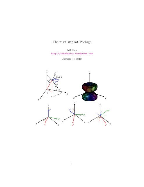
<strong>The</strong> <strong>tikz</strong>-<strong>3dplot</strong> <strong>Package</strong><br />
Jeff Hein<br />
http://<strong>tikz</strong><strong>3dplot</strong>.wordpress.com<br />
January 11, 2012<br />
z<br />
z<br />
φ<br />
θ<br />
z ′ θ ′<br />
φ ′<br />
x ′ y ′<br />
y<br />
x<br />
z<br />
x<br />
z<br />
z<br />
y<br />
x<br />
z ′<br />
y ′<br />
γ<br />
x ′ y<br />
x<br />
z ′<br />
β<br />
y ′<br />
y<br />
x ′<br />
x<br />
α<br />
z ′<br />
x ′ y ′<br />
y<br />
i
Document Version History<br />
2009-11-09 Initial release<br />
2009-11-21 Added spherical polar parametric surface plotting functionality<br />
with the \tdplotsphericalsurfaceplot command.<br />
2009-12-04 Touched up on a few drawing issues in \tdplotsphericalsurfaceplot,<br />
and added the \tdplotshowargcolorguide command.<br />
2010-01-17 Changed package name from <strong>3dplot</strong> to <strong>tikz</strong>-<strong>3dplot</strong>, and updated<br />
document accordingly.<br />
2010-01-20 Added the following commands: \tdplotgetpolarcoords, \tdplotcrossprod,<br />
\tdplotcalctransformrotmain, \tdplotcalctransformmainrot, \tdplottransformrotmain,<br />
\tdplottransformmainrot, and \tdplotdrawpolytopearc.<br />
2010-01-24 Added the ability to hue 3d polar plots based on radius using the<br />
\tdplotr macro.<br />
2010-03-16 Added the \tdplotcalctransformmainscreen and \tdplottransformmainscreen<br />
commands.<br />
2010-04-13 Performed minor bug fixes with \tdplotsphericalsurfaceplot, and<br />
did some slight code cleanup.<br />
2010-07-30 Fixed a bug with using arrowheads in the \tdplotdrawarc command.<br />
Additional arrowheads will no longer be rendered beside the arc<br />
label node.<br />
2011-02-28 Fixed a bug with displaying x and y axes in the \tdplotsphericalsurfaceplot<br />
command.<br />
2011-06-27 Fixed a problem that was causing missing parts when using the<br />
\tdplotsetpolarplotrange command, and fixed minor typos in the documentation.<br />
2012-01-11 Fixed an problem with \tdplotdrawpolytopearc, where arcs were<br />
not drawing properly due to incorrect assessment of comparison statements.<br />
Problem arose due to comparing “1.0” versus “1” in \ifthenelse<br />
statements, so probably a version change issue.<br />
Copyright 2010-2012 Jeff Hein<br />
Permission is granted to distribute and/or modify both the documentation and<br />
the code under the conditions of the LaTeX Project Public License, either<br />
version 1.3 of this license or (at your option) any later version. <strong>The</strong> latest<br />
version of this license is in http://www.latex-project.org/lppl.txt
Contents<br />
Contents<br />
i<br />
1 Introduction 1<br />
1.1 Overview of the <strong>tikz</strong>-<strong>3dplot</strong> <strong>Package</strong> . . . . . . . . . . . . . . 1<br />
1.1.1 What <strong>tikz</strong>-<strong>3dplot</strong> is . . . . . . . . . . . . . . . . . . . 1<br />
1.1.2 What <strong>tikz</strong>-<strong>3dplot</strong> is not . . . . . . . . . . . . . . . . . 2<br />
1.1.3 Similar Work . . . . . . . . . . . . . . . . . . . . . . . . 2<br />
1.2 Installing the <strong>tikz</strong>-<strong>3dplot</strong> <strong>Package</strong> . . . . . . . . . . . . . . . 4<br />
1.2.1 <strong>tikz</strong>-<strong>3dplot</strong> Requirements . . . . . . . . . . . . . . . . 4<br />
1.2.2 <strong>tikz</strong>-<strong>3dplot</strong> <strong>Package</strong> Options . . . . . . . . . . . . . . 4<br />
1.3 Using the <strong>tikz</strong>-<strong>3dplot</strong> <strong>Package</strong> . . . . . . . . . . . . . . . . . 4<br />
2 Overview of 3d in <strong>tikz</strong>-<strong>3dplot</strong> 5<br />
2.1 TikZ 3d Plotting . . . . . . . . . . . . . . . . . . . . . . . . . . 5<br />
2.2 <strong>The</strong> <strong>tikz</strong>-<strong>3dplot</strong> Main Coordinate System . . . . . . . . . . . 5<br />
2.3 <strong>The</strong> <strong>tikz</strong>-<strong>3dplot</strong> Rotated Coordinate System . . . . . . . . . 7<br />
2.4 Arcs in 3d, and the “<strong>The</strong>ta Plane” . . . . . . . . . . . . . . . . 8<br />
3 Using the <strong>tikz</strong>-<strong>3dplot</strong> <strong>Package</strong> 10<br />
3.1 <strong>The</strong> <strong>tikz</strong>-<strong>3dplot</strong> TikZ Styles . . . . . . . . . . . . . . . . . . . 10<br />
3.1.1 tdplot main coords . . . . . . . . . . . . . . . . . . . . 10<br />
3.1.2 tdplot rotated coords . . . . . . . . . . . . . . . . . . 10<br />
3.1.3 tdplot screen coords . . . . . . . . . . . . . . . . . . 10<br />
3.2 <strong>The</strong> <strong>tikz</strong>-<strong>3dplot</strong> Commands . . . . . . . . . . . . . . . . . . . 11<br />
3.3 Coordinate Configuration Commands . . . . . . . . . . . . . . 11<br />
3.3.1 tdplotsetmaincoords . . . . . . . . . . . . . . . . . . . 11<br />
3.3.2 tdplotsetrotatedcoords . . . . . . . . . . . . . . . . . 11<br />
3.3.3 tdplotsetrotatedcoordsorigin . . . . . . . . . . . . . 12<br />
3.3.4 tdplotresetrotatedcoordsorigin . . . . . . . . . . . 13<br />
3.3.5 tdplotsetthetaplanecoords . . . . . . . . . . . . . . . 13<br />
3.3.6 tdplotsetrotatedthetaplanecoords . . . . . . . . . . 14<br />
3.3.7 tdplotcalctransformmainrot . . . . . . . . . . . . . . 16<br />
3.3.8 tdplotcalctransformrotmain . . . . . . . . . . . . . . 16<br />
3.3.9 tdplotcalctransformmainscreen . . . . . . . . . . . . 16<br />
3.4 Point Calculation Commands . . . . . . . . . . . . . . . . . . . 17<br />
i
3.4.1 tdplotsetcoord . . . . . . . . . . . . . . . . . . . . . . 17<br />
3.4.2 tdplottransformmainrot . . . . . . . . . . . . . . . . . 18<br />
3.4.3 tdplottransformrotmain . . . . . . . . . . . . . . . . . 19<br />
3.4.4 tdplottransformmainscreen . . . . . . . . . . . . . . . 21<br />
3.4.5 tdplotgetpolarcoords . . . . . . . . . . . . . . . . . . 22<br />
3.4.6 tdplotcrossprod . . . . . . . . . . . . . . . . . . . . . 23<br />
3.4.7 tdplotdefinepoints . . . . . . . . . . . . . . . . . . . 25<br />
3.5 Drawing Commands . . . . . . . . . . . . . . . . . . . . . . . . 26<br />
3.5.1 tdplotdrawarc . . . . . . . . . . . . . . . . . . . . . . . 26<br />
3.5.2 tdplotdrawpolytopearc . . . . . . . . . . . . . . . . . 28<br />
3.6 <strong>The</strong> tdplotsphericalsurfaceplot Command . . . . . . . . . 30<br />
3.6.1 How tdplotsphericalsurfaceplot Works . . . . . . . 30<br />
3.6.2 Using tdplotsphericalsurfaceplot . . . . . . . . . . 30<br />
3.6.3 <strong>The</strong> tdplotsetpolarplotrange Command . . . . . . . 32<br />
3.6.4 <strong>The</strong> tdplotresetpolarplotrange Command . . . . . . 33<br />
3.6.5 <strong>The</strong> tdplotshowargcolorguide Command . . . . . . . 33<br />
3.7 Miscellaneous Math Commands . . . . . . . . . . . . . . . . . . 34<br />
3.7.1 tdplotsinandcos . . . . . . . . . . . . . . . . . . . . . 34<br />
3.7.2 tdplotmult . . . . . . . . . . . . . . . . . . . . . . . . . 35<br />
3.7.3 tdplotdiv . . . . . . . . . . . . . . . . . . . . . . . . . 35<br />
4 Known Issues 36<br />
4.1 Predefined Points Don’t Work in Rotated Frame . . . . . . . . 36<br />
4.2 node Command and shift=(P) Issues . . . . . . . . . . . . . . 37<br />
4.3 PGF xyz spherical Coordinate System . . . . . . . . . . . . . 39<br />
5 TODO list 40
Chapter 1<br />
Introduction<br />
1.1 Overview of the <strong>tikz</strong>-<strong>3dplot</strong> <strong>Package</strong><br />
<strong>The</strong> <strong>tikz</strong>-<strong>3dplot</strong> package offers commands and coordinate transformation<br />
styles for TikZ, providing relatively straightforward tools to draw three-dimensional<br />
coordinate systems and simple three-dimensional diagrams. <strong>The</strong> package is currently<br />
in its infancy, and is subject to change. Comments or suggestions are<br />
encouraged.<br />
This document describes the basics of the <strong>tikz</strong>-<strong>3dplot</strong> package and provides<br />
information about the various available commands. Examples are given<br />
where possible.<br />
1.1.1 What <strong>tikz</strong>-<strong>3dplot</strong> is<br />
<strong>tikz</strong>-<strong>3dplot</strong> provides commands to easily specify coordinate transformations<br />
for TikZ, allowing for relatively easy plotting. I needed to draw accurate 3d<br />
vector images for a physics thesis, and this package was developed to meet this<br />
need.<br />
Various plotting commands are used to identify coordinate locations using<br />
spherical polar or Cartesian coordinates. Coordinate transformation commands<br />
allow for the calculation of a coordinate in one frame based on its values<br />
in another frame. Some drawing commands have been developed to assist in<br />
the rendering of arcs. <strong>The</strong>se commands do the number crunching required to<br />
position and render the arcs. <strong>The</strong>se commands are discussed in Section 3.2.<br />
In addition, the \tdplotsphericalsurfaceplot was developed to render threedimensional<br />
surfaces in spherical polar coordinates, where the radius is expressed<br />
in terms of a user-defined function of θ and φ. With this function, the<br />
surface hue can be given explicitly, or expressed as a user-defined function of<br />
r, θ, and φ. This command is discussed in Section 3.6.<br />
In <strong>tikz</strong>-<strong>3dplot</strong>, a right-handed coordinate system convention is used. In<br />
addition, all positive angles constitute a right-hand screw sense of rotation (see<br />
Figure 1.1). This means that a positive rotation about a given axis refers to a<br />
1
z<br />
y<br />
x<br />
Figure 1.1: <strong>tikz</strong>-<strong>3dplot</strong> coordinate and positive angle convention.<br />
clockwise rotation when viewing along the direction the axis, or counterclockwise<br />
when viewing against the direction of the axis.<br />
1.1.2 What <strong>tikz</strong>-<strong>3dplot</strong> is not<br />
<strong>tikz</strong>-<strong>3dplot</strong> does not, in general, consider polygons, surfaces, or object opacity.<br />
<strong>The</strong> one exception is the \tdplotsphericalsurfaceplot command, specifically<br />
designed to render spherical polar surfaces. <strong>The</strong> \tdplotsphericalsurfaceplot<br />
command is discussed in Section 3.6.<br />
Tools like Sketch by Gene Ressler are better suited for more rigorous surface<br />
rendering. <strong>The</strong>se can be found at http://www.frontiernet.net/~eugene.<br />
ressler/<br />
1.1.3 Similar Work<br />
To my knowledge, there is no other package available which allows straightforward<br />
rendering of 3d coordinates in TikZ, directly in a L A TEX document. Since<br />
this project is in its infancy, this may be subject to change based on feedback.<br />
Sketch<br />
<strong>The</strong> Sketch project can provide three-dimensional rendering of axes, points,<br />
and lines, but (as far as I understand the program) cannot draw arcs without<br />
using a series of line segments. Further, Sketch requires an external program to<br />
render the image, while <strong>tikz</strong>-<strong>3dplot</strong> can be developed and maintained right<br />
in a L A TEX document.<br />
TEXample.net<br />
<strong>The</strong>re are a variety of TikZ examples listed at http://www.texample.net/<br />
<strong>tikz</strong>/examples. Some of these examples gave me inspiration to make this<br />
package. Some examples of note include the following:<br />
• 3D cone<br />
2
Author: Eugene Ressler<br />
url: http://www.texample.net/<strong>tikz</strong>/examples/3d-cone/<br />
Notes: This demonstrates the use of Sketch in TikZ figures.<br />
• Annotated 3D box<br />
Author Alain Matthes<br />
url http://www.texample.net/<strong>tikz</strong>/examples/annotated-3d-box/<br />
Notes This example demonstrates the direct use of coordinate transformations,<br />
as well as performing math directly within coordinates.<br />
• Cluster of atoms<br />
Author Agustin E. Bolzan<br />
url http://www.texample.net/<strong>tikz</strong>/examples/clusters-of-atoms/<br />
Notes This uses shifts and slants rather than rotations to render an<br />
isometric look.<br />
• Plane partition<br />
Author Jang Soo Kim<br />
url http://www.texample.net/<strong>tikz</strong>/examples/plane-partition/<br />
Notes This example draws solid surfaces with coordinate axes defined<br />
by rotations around the TikZ standard coordinate frame.<br />
• Spherical and cartesian grids<br />
Author Marco Miani<br />
url http://www.texample.net/<strong>tikz</strong>/examples/spherical-and-cartesian-grids/<br />
Notes This example renders arcs and lines in three dimensions using explicit<br />
calculations. It takes into account the opacity of the spherical<br />
example, by showing hidden lines behind the sphere as dashed lines.<br />
• Stereographic and cylindrical map projections<br />
Author Thomas M. Trzeciak<br />
url http://www.texample.net/<strong>tikz</strong>/examples/map-projections/<br />
Notes This example illustrates the use of coordinate transformations to<br />
draw planes and arcs for spherical coordinates.<br />
3
1.2 Installing the <strong>tikz</strong>-<strong>3dplot</strong> <strong>Package</strong><br />
Get a copy of <strong>tikz</strong>-<strong>3dplot</strong> from http://www.ctan.org. Place the style file in<br />
the same directory as your L A TEX project. In your preamble, add the following<br />
line:<br />
\usepackage{<strong>tikz</strong>-<strong>3dplot</strong>}<br />
Make sure this line is written after all other required packages.<br />
1.2.1 <strong>tikz</strong>-<strong>3dplot</strong> Requirements<br />
To use this package, the following other packages must be loaded in the preamble<br />
first:<br />
• TikZ<br />
• ifthen (for the tdplotsphericalsurfaceplot command)<br />
1.2.2 <strong>tikz</strong>-<strong>3dplot</strong> <strong>Package</strong> Options<br />
Currently there are no options available for the <strong>tikz</strong>-<strong>3dplot</strong> package.<br />
1.3 Using the <strong>tikz</strong>-<strong>3dplot</strong> <strong>Package</strong><br />
<strong>tikz</strong>-<strong>3dplot</strong> provides styles and commands which are useful in a <strong>tikz</strong>picture<br />
environment. <strong>The</strong>se commands and styles are described in Chapter 3.<br />
4
Chapter 2<br />
Overview of 3d in <strong>tikz</strong>-<strong>3dplot</strong><br />
2.1 TikZ 3d Plotting<br />
When setting up a <strong>tikz</strong>picture or a drawing style, the x, y, and z axes can<br />
be specified directly in terms of the original coordinate system. <strong>The</strong> following<br />
example shows how a <strong>tikz</strong>picture environment can be configured to use<br />
customized axes.<br />
\begin{<strong>tikz</strong>picture}[%<br />
x={(\raarot cm,\rbarot cm)},%<br />
y={(\rabrot cm, \rbbrot cm)},%<br />
z={(\racrot, \rbcrot cm)}]<br />
In this example, the terms \raarot and so on specify how the coordinates<br />
are represented in the original TikZ coordinate system, and are calculated<br />
by the <strong>tikz</strong>-<strong>3dplot</strong> package. Note that units are explicitly required so TikZ<br />
understands that these are absolute coordinates, not scales on the existing axis.<br />
See the PGF manual Version 2.00, section 21.2 on pages 217-218 for details on<br />
TikZ coordinate transformations.<br />
2.2 <strong>The</strong> <strong>tikz</strong>-<strong>3dplot</strong> Main Coordinate System<br />
<strong>tikz</strong>-<strong>3dplot</strong> offers two coordinate systems, namely the main coordinate system<br />
(x, y, z), and the rotated coordinate system (x ′ , y ′ , z ′ ). <strong>The</strong> latter system<br />
is described in Section 2.3.<br />
As the name suggests, the main coordinate system provides a user-specified<br />
transformation to render 3d points in a <strong>tikz</strong>picture environment. <strong>The</strong> orientation<br />
of the main coordinate system is defined by the angles θ d and φ d . In the<br />
unrotated (θ d = φ d = 0) position, the xy plane of the main coordinate system<br />
coincides with the default orientation for a <strong>tikz</strong>picture environment, while z<br />
5
points “out of the page”. <strong>The</strong> coordinate system is positioned by the following<br />
operations:<br />
• Rotate the coordinate system about the body x axis by the amount θ d ,<br />
and<br />
• Rotate the coordinate system about the (rotated) body z axis by the<br />
amount φ d .<br />
In this rotation sense, the z axis will always point in the vertical page<br />
direction. This transformation is given by the rotation matrix R d (θ d , φ d ), as<br />
R d (θ d , φ d ) = R z′ (φ d )R x (θ d )<br />
⎛<br />
⎞ ⎛<br />
⎞<br />
cos φ d − sin φ d 0 1 0 0<br />
= ⎝sin φ d cos φ d 0⎠<br />
⎝0 cos θ d − sin θ d<br />
⎠<br />
0 0 1 0 sin θ d cos θ d<br />
⎛<br />
⎞<br />
cos φ d sin φ d 0<br />
= ⎝− cos θ d sin φ d cos θ d cos φ d − sin θ d<br />
⎠<br />
sin θ d sin φ d − sin θ d cos φ d cos θ d<br />
(2.1)<br />
Using this matrix, the TikZ coordinate transformation can be applied as<br />
described in Section 2.1 by the various matrix elements, as<br />
x = (R d 1,1, R d 2,1)<br />
y = (R d 1,2, R d 2,2)<br />
z = (R d 1,3, R d 2,3)<br />
(2.2)<br />
Note that the third row of the rotation matrix is not needed for this transformation,<br />
since a screen coordinate is a 2d value. Once the transformed axes<br />
have been established, any 3d coordinate specified in TikZ will adhere to the<br />
y<br />
z<br />
x<br />
z<br />
z<br />
x<br />
y<br />
z<br />
x<br />
z<br />
y<br />
z<br />
x<br />
y<br />
x<br />
y<br />
x<br />
y<br />
Figure 2.1: Examples of coordinate systems for various choices of θ d and φ d .<br />
6
transformation, yielding a 3D representation. Lines and nodes can readily be<br />
drawn by using these 3d coordinates.<br />
This coordinate transformation is accessible through <strong>tikz</strong>-<strong>3dplot</strong> using<br />
the command tdplotsetmaincoords, as described in Chapter 3.<br />
2.3 <strong>The</strong> <strong>tikz</strong>-<strong>3dplot</strong> Rotated Coordinate System<br />
Along with the main coordinate system, described in Section 2.2, <strong>tikz</strong>-<strong>3dplot</strong><br />
offers a rotated coordinate system that is defined with respect to the main<br />
coordinate system. This system can be rotated to any position using Euler<br />
rotations, and can be translated so the origin of the rotated coordinate system<br />
sits on an arbitrary point in the main coordinate system.<br />
Three rotations can be performed to give any arbitrary orientation of a<br />
rotated coordinate system. By convention, the following rotations are chosen:<br />
• Rotate by angle γ about the world z axis,<br />
• Rotate by angle β about the (unrotated) world y axis, and<br />
• Rotate by angle α about the (unrotated) world z axis.<br />
<strong>The</strong>se rotations are shown in Figure 2.2.<br />
z<br />
z<br />
z<br />
x<br />
z ′<br />
y ′<br />
γ<br />
x ′ y<br />
x<br />
z ′<br />
β<br />
y ′<br />
y<br />
x ′<br />
x<br />
α<br />
z ′<br />
x ′ y ′<br />
y<br />
Figure 2.2: Positioning the rotated coordinate frame (x ′ , y ′ , z ′ ) using Euler<br />
angles (α, β, γ).<br />
This rotation matrix D(α, β, γ) is given by<br />
D(α, β, γ) = R z (α)R y (β)R z (γ)<br />
⎛<br />
⎞ ⎛<br />
⎞ ⎛<br />
⎞<br />
cos α − sin α 0 cos β 0 sin β cos γ − sin γ 0<br />
= ⎝sin α cos α 0⎠<br />
⎝ 0 1 0 ⎠ ⎝sin γ cos γ 0⎠<br />
0 0 1 − sin β 0 cos β 0 0 1<br />
⎛<br />
⎞<br />
cos α cos β cos γ − sin α sin γ − cos α cos β sin γ − sin α cos γ cos α sin β<br />
= ⎝sin α cos β cos γ + cos α sin γ − sin α cos β sin γ + cos α cos γ sin α sin β⎠<br />
− sin β cos γ sin β sin γ cos β<br />
(2.3)<br />
7
To define the rotated coordinate frame, this rotation matrix is applied after<br />
rotation matrix R d (θ d , φ d ) used to define the main coordinate frame. <strong>The</strong> full<br />
transformation for the rotated coordinate frame is then given by<br />
R ′d (θ d , φ d , α, β, γ) = D(α, β, γ)R d (θ d , φ d ) (2.4)<br />
Using this matrix, the TikZ coordinate transformation can be applied as<br />
described in Section 2.1 by the various matrix elements, as<br />
x ′ = (R ′d<br />
1,1, R ′d<br />
2,1)<br />
y ′ = (R ′d<br />
1,2, R ′d<br />
2,2)<br />
z ′ = (R ′d<br />
1,3, R ′d<br />
2,3)<br />
(2.5)<br />
This coordinate transformation is accessible through <strong>tikz</strong>-<strong>3dplot</strong> using<br />
the command tdplotsetrotatedcoords, as described in Chapter 3.<br />
z<br />
z ′<br />
x<br />
x ′ y ′<br />
y<br />
Figure 2.3: <strong>The</strong> rotated coordinate frame (x ′ , y ′ , z ′ ) displayed within the main<br />
coordinate frame (x, y, z). Both are completely specified by user-defined angles:<br />
(θ d , φ d ) for the main coordinate frame, and (α, β, γ) for the rotated coordinate<br />
frame.<br />
2.4 Arcs in 3d, and the “<strong>The</strong>ta Plane”<br />
Arcs can be drawn in TikZ using commands described in the PGF manual<br />
Version 2.00, section 2.10 on pages 25-26. However, the arc commands accept<br />
2d coordinates, and thus can only be drawn in the xy plane.<br />
8
To draw an arc in any position other than within the xy plane of the main<br />
coordinate frame, the rotated coordinate frame must be used, where the x ′ y ′<br />
plane lies in the desired orientation within the main coordinate frame. Such an<br />
arc is needed, for example, when illustrating the polar angle θ of some vector.<br />
This θ arc exists in a plane which contains the z axis, and is rotated about the<br />
z axis by the angle φ from the xz plane. For lack of a better name, this plane<br />
is referred to as the “theta plane” within a given coordinate system.<br />
z<br />
θ<br />
x ′ y ′ z ′<br />
y<br />
x<br />
Figure 2.4: Drawing arcs outside the xy plane by using a rotated coordinate<br />
frame in the “theta plane” of the main coordinate frame.<br />
As described in Chapter 3, <strong>tikz</strong>-<strong>3dplot</strong> offers the commands tdplotsetthetaplanecoords<br />
and tdplotsetrotatedthetaplanecoords to easily configure the rotated coordinate<br />
frame to lie within the desired theta plane.<br />
9
Chapter 3<br />
Using the <strong>tikz</strong>-<strong>3dplot</strong> <strong>Package</strong><br />
<strong>The</strong> <strong>tikz</strong>-<strong>3dplot</strong> package was developed to handle the number crunching described<br />
in Chapter 2, and provide a relatively simple and straightforward frontend<br />
for users.<br />
<strong>The</strong> main and rotated coordinate frames are configured by using commands<br />
described in Section 3.2. <strong>The</strong>se commands generate TikZ styles which can be<br />
used either in defining the <strong>tikz</strong>picture environment, or directly in any TikZ<br />
command. <strong>The</strong> styles are described further in Section 3.1.<br />
3.1 <strong>The</strong> <strong>tikz</strong>-<strong>3dplot</strong> TikZ Styles<br />
3.1.1 tdplot main coords<br />
<strong>The</strong> tdplot_main_coords style stores the coordinate transformation required to<br />
generate the main coordinate system. This style can either be used when<br />
the <strong>tikz</strong>picture environment is started, or when an individual TikZ plotting<br />
command is used.<br />
3.1.2 tdplot rotated coords<br />
<strong>The</strong> tdplot_rotated_coords style stores the coordinate transformation (translation<br />
and rotation) required to generate the rotated coordinate system within<br />
the main coordinate system. This style can either be used when the <strong>tikz</strong>picture<br />
environment is started, or when an individual TikZ plotting command is used.<br />
3.1.3 tdplot screen coords<br />
<strong>The</strong> tdplot_screen_coords style provides the standard, unrotated TikZ coordinate<br />
frame. This is useful to escape out of the user-defined 3d coordinates used<br />
at the beginning of the <strong>tikz</strong>picture environment, and place something on an<br />
absolute scale in the figure. Tables, legends, and captions contained within the<br />
same figure as a 3d plot can make use of this style.<br />
10
3.2 <strong>The</strong> <strong>tikz</strong>-<strong>3dplot</strong> Commands<br />
This section lists the various commands provided by the <strong>tikz</strong>-<strong>3dplot</strong> package.<br />
Examples are provided where it is useful.<br />
3.3 Coordinate Configuration Commands<br />
3.3.1 tdplotsetmaincoords<br />
Description: Generates the style tdplot_main_coords which provides the coordinate<br />
transformation for the main coordinate frame, based on a userspecified<br />
orientation (θ d , φ d ). θ d denotes the rotation around the x axis,<br />
while φ d denotes the rotation around the z axis. Note that (0, 0) is the<br />
default orientation, where x points right, y points up, and z points “out<br />
of the page”.<br />
Syntax: \tdplotsetmaincoords{ θ d }{ φ d }<br />
Parameters:<br />
θ d<br />
φ d<br />
<strong>The</strong> angle (in degrees) through which the coordinate frame is rotated<br />
about the x axis.<br />
<strong>The</strong> angle (in degrees) through which the coordinate frame is rotated<br />
about the z axis.<br />
Example:<br />
\tdplotsetmaincoords{70}{110}<br />
\begin{<strong>tikz</strong>picture}[tdplot_main_coords]<br />
\draw[thick,->] (0,0,0) -- (1,0,0) node[anchor=north east]{$x$};<br />
\draw[thick,->] (0,0,0) -- (0,1,0) node[anchor=north west]{$y$};<br />
\draw[thick,->] (0,0,0) -- (0,0,1) node[anchor=south]{$z$};<br />
\end{<strong>tikz</strong>picture}<br />
z<br />
x<br />
y<br />
3.3.2 tdplotsetrotatedcoords<br />
Description: Generates the style tdplot_rotated_coords which provides the coordinate<br />
transformation for rotated coordinate frame within the current<br />
main coordinate frame, based on user-specified Euler angles (α, β, γ).<br />
Rotations use the z(α)y(β)z(γ) convention of Euler rotations, where the<br />
11
system is rotated by γ about the z axis, then β about the (world) y axis,<br />
and then α about the (world) z axis.<br />
Syntax: \tdplotsetrotatedcoords{α}{β}{γ}<br />
Parameters:<br />
Example:<br />
α <strong>The</strong> angle (in degrees) through which the rotated frame is rotated<br />
about the world z axis.<br />
β <strong>The</strong> angle (in degrees) through which the rotated frame is rotated<br />
about the world y axis.<br />
γ <strong>The</strong> angle (in degrees) through which the rotated frame is rotated<br />
about the world z axis.<br />
\tdplotsetmaincoords{70}{110}<br />
\begin{<strong>tikz</strong>picture}[tdplot_main_coords]<br />
\draw[thick,->] (0,0,0) -- (1,0,0) node[anchor=north east]{$x$};<br />
\draw[thick,->] (0,0,0) -- (0,1,0) node[anchor=north west]{$y$};<br />
\draw[thick,->] (0,0,0) -- (0,0,1) node[anchor=south]{$z$};<br />
\tdplotsetrotatedcoords{60}{40}{30}<br />
\draw[thick,color=blue,tdplot_rotated_coords,->] (0,0,0) --<br />
(.7,0,0) node[anchor=north]{$x’$};<br />
\draw[thick,color=blue,tdplot_rotated_coords,->] (0,0,0) --<br />
(0,.7,0) node[anchor=west]{$y’$};<br />
\draw[thick,color=blue,tdplot_rotated_coords,->] (0,0,0) --<br />
(0,0,.7) node[anchor=south]{$z’$};<br />
\end{<strong>tikz</strong>picture}<br />
z<br />
z ′ y ′<br />
x<br />
x ′<br />
y<br />
3.3.3 tdplotsetrotatedcoordsorigin<br />
Description: Sets the origin of the rotated coordinate system specified by<br />
tdplot_rotated_coords using a user-defined point. This point can be either<br />
a literal or predefined point.<br />
Syntax: \tdplotsetrotatedcoordsorigin{point}<br />
Parameters:<br />
point A point predefined using the TikZ \coordinate command.<br />
12
Example:<br />
\tdplotsetmaincoords{70}{110}<br />
\begin{<strong>tikz</strong>picture}[tdplot_main_coords]<br />
\draw[thick,->] (0,0,0) -- (1,0,0) node[anchor=north east]{$x$};<br />
\draw[thick,->] (0,0,0) -- (0,1,0) node[anchor=north west]{$y$};<br />
\draw[thick,->] (0,0,0) -- (0,0,1) node[anchor=south]{$z$};<br />
\tdplotsetrotatedcoords{60}{40}{30}<br />
\coordinate (Shift) at (0.5,0.5,0.5);<br />
\tdplotsetrotatedcoordsorigin{(Shift)}<br />
\draw[thick,color=blue,tdplot_rotated_coords,->] (0,0,0) --<br />
(.7,0,0) node[anchor=north]{$x’$};<br />
\draw[thick,color=blue,tdplot_rotated_coords,->] (0,0,0) --<br />
(0,.7,0) node[anchor=west]{$y’$};<br />
\draw[thick,color=blue,tdplot_rotated_coords,->] (0,0,0) --<br />
(0,0,.7) node[anchor=south]{$z’$};<br />
\end{<strong>tikz</strong>picture}<br />
z<br />
z ′ y ′<br />
x<br />
x ′<br />
y<br />
3.3.4 tdplotresetrotatedcoordsorigin<br />
Description: Resets the origin of the rotated coordinate system back to the<br />
origin of the main coordinate system.<br />
Syntax: \tdplotresetrotatedcoordsorigin<br />
Parameters: None<br />
3.3.5 tdplotsetthetaplanecoords<br />
Description: Generates a rotated coordinate system such that the x ′ y ′ plane<br />
is coplanar to a plane containing the polar angle θ projecting from the<br />
main coordinate system z axis. This coordinate system is particularly<br />
useful for drawing within this “theta plane”, as TikZ draws arcs in the xy<br />
plane. As with tdplotsetrotatedcoords, this coordinate system is accessible<br />
through the tdplot_rotated_coords style. Note that any rotated coordinate<br />
frame offset previously set by tdplotsetrotatedcoordsorigin<br />
is automatically reset when this command is used.<br />
Syntax: \tdplotsetthetaplanecoords{φ}<br />
Parameters:<br />
13
φ <strong>The</strong> angle (in degrees) through which the “theta plane” makes with<br />
the xz plane of the main coordinate system.<br />
Example:<br />
\tdplotsetmaincoords{70}{110}<br />
\begin{<strong>tikz</strong>picture}[scale=3,tdplot_main_coords]<br />
\draw[thick,->] (0,0,0) -- (1,0,0) node[anchor=north east]{$x$};<br />
\draw[thick,->] (0,0,0) -- (0,1,0) node[anchor=north west]{$y$};<br />
\draw[thick,->] (0,0,0) -- (0,0,1) node[anchor=south]{$z$};<br />
\tdplotsetcoord{P}{.8}{50}{70}<br />
%draw a vector from origin to point (P)<br />
\draw[-stealth,color=red] (O) -- (P);<br />
%draw projection on xy plane, and a connecting line<br />
\draw[dashed, color=red] (O) -- (Pxy);<br />
\draw[dashed, color=red] (P) -- (Pxy);<br />
\tdplotsetthetaplanecoords{70}<br />
\draw[tdplot_rotated_coords,color=blue,thick,->] (0,0,0)<br />
-- (.2,0,0) node[anchor=east]{$x’$};<br />
\draw[tdplot_rotated_coords,color=blue,thick,->] (0,0,0)<br />
-- (0,.2,0) node[anchor=north]{$y’$};<br />
\draw[tdplot_rotated_coords,color=blue,thick,->] (0,0,0)<br />
-- (0,0,.2) node[anchor=west]{$z’$};<br />
\end{<strong>tikz</strong>picture}<br />
z<br />
x ′ y ′ z ′<br />
x<br />
y<br />
3.3.6 tdplotsetrotatedthetaplanecoords<br />
Description: Just like tdplotsetthetaplanecoords, except this works for<br />
the rotated coordinate system. Generates a rotated coordinate system<br />
such that the x ′ − y ′ plane is coplanar to a plane containing the polar<br />
14
angle θ ′ projecting from the current rotated coordinate system z ′ axis.<br />
Note that the current rotated coordinate system is overwritten by this<br />
theta plane coordinate system after the command is completed.<br />
Syntax: \tdplotsetrotatedthetaplanecoords{φ ′ }<br />
Parameters:<br />
φ ′<br />
<strong>The</strong> angle (in degrees) through which the “theta plane” makes with<br />
the x ′ − z ′ plane of the current rotated coordinate system.<br />
Example:<br />
\tdplotsetmaincoords{60}{110}<br />
\begin{<strong>tikz</strong>picture}[scale=3,tdplot_main_coords]<br />
\draw[thick,->] (0,0,0) -- (1,0,0) node[anchor=north east]{$x$};<br />
\draw[thick,->] (0,0,0) -- (0,1,0) node[anchor=north west]{$y$};<br />
\draw[thick,->] (0,0,0) -- (0,0,1) node[anchor=south]{$z$};<br />
\coordinate (Shift) at (2,2,2);<br />
\tdplotsetrotatedcoords{-20}{10}{0}<br />
\tdplotsetrotatedcoordsorigin{(Shift)}<br />
\draw[thick,color=blue,tdplot_rotated_coords,->] (0,0,0)<br />
-- (1,0,0) node[anchor=south east]{$x’$};<br />
\draw[thick,color=blue,tdplot_rotated_coords,->] (0,0,0)<br />
-- (0,1,0) node[anchor=west]{$y’$};<br />
\draw[thick,color=blue,tdplot_rotated_coords,->] (0,0,0)<br />
-- (0,0,1) node[anchor=south]{$z’$};<br />
\tdplotsetrotatedthetaplanecoords{30}<br />
\draw[thick,color=blue,tdplot_rotated_coords,->] (0,0,0)<br />
-- (.5,0,0) node[anchor=south east]{$x’’$};<br />
\draw[thick,color=blue,tdplot_rotated_coords,->] (0,0,0)<br />
-- (0,.5,0) node[anchor=west]{$y’’$};<br />
\draw[thick,color=blue,tdplot_rotated_coords,->] (0,0,0)<br />
-- (0,0,.5) node[anchor=south]{$z’’$};<br />
\end{<strong>tikz</strong>picture}<br />
15
z ′<br />
z<br />
x ′′ y ′′ z ′′<br />
x ′ y ′<br />
y<br />
x<br />
3.3.7 tdplotcalctransformmainrot<br />
Description: Calculates the rotation matrix used to transform a coordinate<br />
from the main coordinate frame to the rotated coordinate frame. <strong>The</strong><br />
matrix elements are stored in the macros \raaeul through \rcceul. This<br />
transformation is accessed using \tdplottransformmainrot.<br />
3.3.8 tdplotcalctransformrotmain<br />
Description: Calculates the rotation matrix used to define the rotated coordinate<br />
frame, as well as transform a coordinate from the rotated coordinate<br />
frame to the main coordinate frame. <strong>The</strong> matrix elements<br />
are stored in the macros \raaeul through \rcceul. This transformation<br />
is used in the \tdplotsetrotatedcoords command, and is accessed using<br />
\tdplottransformrotmain.<br />
3.3.9 tdplotcalctransformmainscreen<br />
Description: Calculates the rotation matrix used to define the main coordinate<br />
frame, as well as transform a coordinate from the main coordinate<br />
frame to the screen coordinate frame. <strong>The</strong> matrix elements are stored in<br />
the macros \raarot through \rccrot. This transformation is used in the<br />
\tdplotsetmaincoords command, and is accessed using \tdplottransformmainscreen.<br />
16
3.4 Point Calculation Commands<br />
3.4.1 tdplotsetcoord<br />
Description: Generates a TikZ coordinate of specified name, along with coordinates<br />
for the x−, y−, z−, xy−, xz−, and yz− projections of the<br />
coordinate, based on user-specified spherical coordinates. Note that this<br />
coordinate only works in the main coordinate system. All points in the<br />
rotated coordinate system must be specified as literal points.<br />
Syntax: \tdplotsetcoord{point}{r}{θ}{φ}<br />
Parameters:<br />
Example:<br />
point <strong>The</strong> name of the TikZ coordinate to be assigned. Note that the<br />
() parentheses must be excluded.<br />
r Point radius.<br />
θ Point polar angle.<br />
φ Point azimuthal angle.<br />
\tdplotsetmaincoords{60}{130}<br />
\begin{<strong>tikz</strong>picture}[scale=2,tdplot_main_coords]<br />
\coordinate (O) at (0,0,0);<br />
\tdplotsetcoord{P}{.8}{55}{60}<br />
\draw[thick,->] (0,0,0) -- (1,0,0) node[anchor=north east]{$x$};<br />
\draw[thick,->] (0,0,0) -- (0,1,0) node[anchor=north west]{$y$};<br />
\draw[thick,->] (0,0,0) -- (0,0,1) node[anchor=south]{$z$};<br />
\draw[-stealth,color=red] (O) -- (P);<br />
\draw[dashed, color=red] (O) -- (Px);<br />
\draw[dashed, color=red] (O) -- (Py);<br />
\draw[dashed, color=red] (O) -- (Pz);<br />
\draw[dashed, color=red] (Px) -- (Pxy);<br />
\draw[dashed, color=red] (Py) -- (Pxy);<br />
\draw[dashed, color=red] (Px) -- (Pxz);<br />
\draw[dashed, color=red] (Pz) -- (Pxz);<br />
\draw[dashed, color=red] (Py) -- (Pyz);<br />
\draw[dashed, color=red] (Pz) -- (Pyz);<br />
\draw[dashed, color=red] (Pxy) -- (P);<br />
\draw[dashed, color=red] (Pxz) -- (P);<br />
\draw[dashed, color=red] (Pyz) -- (P);<br />
\end{<strong>tikz</strong>picture}<br />
17
z<br />
x<br />
y<br />
3.4.2 tdplottransformmainrot<br />
Description: Transforms a coordinate from the main coordinate frame to the<br />
rotated coordinate frame. This command cannot use a TikZ coordinate,<br />
and does not account for a shifted rotated coordinate frame. <strong>The</strong> results<br />
are stored in the \tdplotresx, \tdplotresy, and \tdplotresz macros.<br />
Syntax: \tdplottransformmainrot{x}{y}{z}<br />
Parameters:<br />
x <strong>The</strong> x-component of the coordinate in the main coordinate frame.<br />
y <strong>The</strong> y-component of the coordinate in the main coordinate frame.<br />
z <strong>The</strong> z-component of the coordinate in the main coordinate frame.<br />
Output: <strong>The</strong> following macros are assigned:<br />
Example:<br />
tdplotresx <strong>The</strong> transformed coordinate x component in the rotated coordinate<br />
frame.<br />
tdplotresy <strong>The</strong> transformed coordinate y component in the rotated coordinate<br />
frame.<br />
tdplotresz <strong>The</strong> transformed coordinate z component in the rotated coordinate<br />
frame.<br />
\tdplotsetmaincoords{50}{140}<br />
\begin{<strong>tikz</strong>picture}[scale=2,tdplot_main_coords]<br />
\draw[thick,->] (0,0,0) -- (1,0,0) node[anchor=north east]{$x$};<br />
\draw[thick,->] (0,0,0) -- (0,1,0) node[anchor=north west]{$y$};<br />
\draw[thick,->] (0,0,0) -- (0,0,1) node[anchor=south]{$z$};<br />
\pgfmathsetmacro{\ax}{2}<br />
\pgfmathsetmacro{\ay}{2}<br />
\pgfmathsetmacro{\az}{1}<br />
18
\tdplotsetrotatedcoords{20}{40}{00}<br />
\draw[thick,color=red,tdplot_rotated_coords,->] (0,0,0)<br />
-- (.7,0,0) node[anchor=east]{$x’$};<br />
\draw[thick,color=green!50!black,tdplot_rotated_coords,->] (0,0,0)<br />
-- (0,.7,0) node[anchor=west]{$y’$};<br />
\draw[thick,color=blue,tdplot_rotated_coords,->] (0,0,0)<br />
-- (0,0,.7) node[anchor=south]{$z’$};<br />
\tdplottransformmainrot{\ax}{\ay}{\az}<br />
\draw[tdplot_rotated_coords,->,blue!50] (0,0,0)<br />
-- (\tdplotresx,\tdplotresy,\tdplotresz);<br />
\node[tdplot_main_coords,anchor=south]<br />
at (\ax,\ay,\az){Main coords: (\ax, \ay, \az)};<br />
\node[tdplot_rotated_coords,anchor=north]<br />
at (\tdplotresx,\tdplotresy,\tdplotresz)<br />
{Rotated coords: (\tdplotresx, \tdplotresy, \tdplotresz)};<br />
\end{<strong>tikz</strong>picture}<br />
z<br />
z ′<br />
y ′<br />
x<br />
x ′ y<br />
Main coords: (2.0, 2.0, 1.0)<br />
Rotated coords: (1.32086, 1.19534, 2.41377)<br />
3.4.3 tdplottransformrotmain<br />
Description: Transforms a coordinate from the rotated coordinate frame to<br />
the main coordinate frame. This command cannot use a TikZ coordinate,<br />
and does not account for a shifted rotated coordinate frame. <strong>The</strong> results<br />
are stored in the \tdplotresx, \tdplotresy, and \tdplotresz macros.<br />
Syntax: \tdplottransformrotmain{x}{y}{z}<br />
Parameters:<br />
x <strong>The</strong> x-component of the coordinate in the rotated coordinate frame.<br />
y <strong>The</strong> y-component of the coordinate in the rotated coordinate frame.<br />
z <strong>The</strong> z-component of the coordinate in the rotated coordinate frame.<br />
19
Output: <strong>The</strong> following macros are assigned:<br />
Example:<br />
tdplotresx <strong>The</strong> transformed coordinate x component in the main coordinate<br />
frame.<br />
tdplotresy <strong>The</strong> transformed coordinate y component in the main coordinate<br />
frame.<br />
tdplotresz <strong>The</strong> transformed coordinate z component in the main coordinate<br />
frame.<br />
\tdplotsetmaincoords{50}{140}<br />
\begin{<strong>tikz</strong>picture}[scale=2,tdplot_main_coords]<br />
\draw[thick,->] (0,0,0) -- (1,0,0) node[anchor=north east]{$x$};<br />
\draw[thick,->] (0,0,0) -- (0,1,0) node[anchor=north west]{$y$};<br />
\draw[thick,->] (0,0,0) -- (0,0,1) node[anchor=south]{$z$};<br />
\pgfmathsetmacro{\ax}{-.75}<br />
\pgfmathsetmacro{\ay}{2.5}<br />
\pgfmathsetmacro{\az}{0}<br />
\tdplotsetrotatedcoords{20}{40}{00}<br />
\draw[thick,color=red,tdplot_rotated_coords,->] (0,0,0)<br />
-- (.7,0,0) node[anchor=east]{$x’$};<br />
\draw[thick,color=green!50!black,tdplot_rotated_coords,->] (0,0,0)<br />
-- (0,.7,0) node[anchor=west]{$y’$};<br />
\draw[thick,color=blue,tdplot_rotated_coords,->] (0,0,0)<br />
-- (0,0,.7) node[anchor=south]{$z’$};<br />
\tdplottransformrotmain{\ax}{\ay}{\az}<br />
\draw[tdplot_main_coords,->,blue!50] (0,0,0)<br />
-- (\tdplotresx,\tdplotresy,\tdplotresz);<br />
\node[tdplot_rotated_coords,anchor=north]<br />
at (\ax,\ay,\az){Rotated coords: (\ax, \ay, \az)};<br />
\node[tdplot_main_coords,anchor=south]<br />
at (\tdplotresx,\tdplotresy,\tdplotresz)<br />
{Main coords: (\tdplotresx, \tdplotresy, \tdplotresz)};<br />
\end{<strong>tikz</strong>picture}<br />
20
z<br />
x<br />
z ′ Main coords: (-1.39493, 2.15276, 0.48209)<br />
y ′ Rotated coords: (-0.75, 2.5, 0.0)<br />
x ′ y<br />
3.4.4 tdplottransformmainscreen<br />
Description: Transforms a coordinate from the main coordinate frame to the<br />
screen coordinate frame. This command cannot use a TikZ coordinate.<br />
<strong>The</strong> results are stored in the \tdplotresx and \tdplotresy macros.<br />
Syntax: \tdplottransformmainscreen{x}{y}{z}<br />
Parameters:<br />
x <strong>The</strong> x-component of the coordinate in the main coordinate frame.<br />
y <strong>The</strong> y-component of the coordinate in the main coordinate frame.<br />
z <strong>The</strong> z-component of the coordinate in the main coordinate frame.<br />
Output: <strong>The</strong> following macros are assigned:<br />
Example:<br />
tdplotresx <strong>The</strong> transformed coordinate x component in the screen coordinate<br />
frame.<br />
tdplotresy <strong>The</strong> transformed coordinate y component in the screen coordinate<br />
frame.<br />
\tdplotsetmaincoords{50}{140}<br />
\begin{<strong>tikz</strong>picture}[scale=2,tdplot_main_coords]<br />
\draw[thick,->] (0,0,0) -- (1,0,0) node[anchor=north east]{$x$};<br />
\draw[thick,->] (0,0,0) -- (0,1,0) node[anchor=north west]{$y$};<br />
\draw[thick,->] (0,0,0) -- (0,0,1) node[anchor=south]{$z$};<br />
\pgfmathsetmacro{\ax}{2}<br />
\pgfmathsetmacro{\ay}{3}<br />
\pgfmathsetmacro{\az}{1}<br />
\tdplottransformmainscreen{\ax}{\ay}{\az}<br />
\draw[tdplot_screen_coords,->,blue!50] (0,0)<br />
21
-- (\tdplotresx,\tdplotresy);<br />
\node[tdplot_main_coords,anchor=south]<br />
at (\ax,\ay,\az){Main coords: (\ax, \ay, \az)};<br />
\node[tdplot_screen_coords,anchor=north]<br />
at (\tdplotresx,\tdplotresy)<br />
{Screen coords: (\tdplotresx, \tdplotresy)};<br />
\end{<strong>tikz</strong>picture}<br />
z<br />
x<br />
y<br />
Main coords: (2.0, 3.0, 1.0)<br />
Screen coords: (0.3963, -1.53752)<br />
3.4.5 tdplotgetpolarcoords<br />
Description: Calculates the θ polar coordinate for the specified point. <strong>The</strong><br />
result is specified in the \tdplotrestheta macro.<br />
Syntax: \tdplotgetpolarcoords{x}{y}{z}<br />
Parameters:<br />
x <strong>The</strong> x-component of the coordinate.<br />
y <strong>The</strong> y-component of the coordinate.<br />
z <strong>The</strong> z-component of the coordinate.<br />
Output: tdplotrestheta <strong>The</strong> θ polar coordinate.<br />
Example:<br />
tdplotresphi <strong>The</strong> φ polar coordinate.<br />
\tdplotsetmaincoords{70}{110}<br />
\begin{<strong>tikz</strong>picture}[tdplot_main_coords]<br />
\draw[thick,->] (0,0,0) -- (3,0,0) node[anchor=north east]{$x$};<br />
22
\draw[thick,->] (0,0,0) -- (0,3,0) node[anchor=north west]{$y$};<br />
\draw[thick,->] (0,0,0) -- (0,0,3) node[anchor=south]{$z$};<br />
\pgfmathsetmacro{\ax}{1}<br />
\pgfmathsetmacro{\ay}{1}<br />
\pgfmathsetmacro{\az}{1}<br />
\draw[->,red] (0,0,0) -- (\ax,\ay,\az);<br />
\draw[dashed,red] (0,0,0) -- (\ax,\ay,0) -- (\ax,\ay,\az);<br />
\tdplotgetpolarcoords{\ax}{\ay}{\az}<br />
\tdplotsetthetaplanecoords{\tdplotresphi}<br />
\tdplotdrawarc[tdplot_rotated_coords]{(0,0,0)}{1}{0}%<br />
{\tdplotrestheta}{anchor=west}{$\theta = \tdplotrestheta$}<br />
\end{<strong>tikz</strong>picture}<br />
z<br />
θ = 54.68636<br />
x<br />
φ = 45.0<br />
y<br />
3.4.6 tdplotcrossprod<br />
Description: Calculates the cross product of two vectors specified by two<br />
coordinates with respect to the origin. <strong>The</strong> result vector is specified by<br />
the coordinates \tdplotresx, \tdplotresy, and \tdplotresz with respect to<br />
the origin.<br />
Syntax: \tdplotcrossprod(a x ,a y ,a z )(b x ,b y ,b z )<br />
Parameters:<br />
a x<br />
a y<br />
a z<br />
b x<br />
b y<br />
<strong>The</strong> x-component of the first vector with respect to the origin.<br />
<strong>The</strong> y-component of the first vector with respect to the origin.<br />
<strong>The</strong> z-component of the first vector with respect to the origin.<br />
<strong>The</strong> x-component of the second vector with respect to the origin.<br />
<strong>The</strong> y-component of the second vector with respect to the origin.<br />
23
z<br />
<strong>The</strong> z-component of the second vector with respect to the origin.<br />
Output: <strong>The</strong> following macros are assigned.<br />
Example:<br />
tdplotresx <strong>The</strong> x-component of the cross product with respect to the<br />
origin.<br />
tdplotresy <strong>The</strong> y-component of the cross product with respect to the<br />
origin.<br />
tdplotresz <strong>The</strong> z-component of the cross product with respect to the<br />
origin.<br />
\tdplotsetmaincoords{50}{110}<br />
\begin{<strong>tikz</strong>picture}[tdplot_main_coords]<br />
\draw[thick,->] (0,0,0) -- (3,0,0) node[anchor=north east]{$x$};<br />
\draw[thick,->] (0,0,0) -- (0,3,0) node[anchor=north west]{$y$};<br />
\draw[thick,->] (0,0,0) -- (0,0,3) node[anchor=south]{$z$};<br />
\pgfmathsetmacro{\ax}{1}<br />
\pgfmathsetmacro{\ay}{1}<br />
\pgfmathsetmacro{\az}{.4}<br />
\pgfmathsetmacro{\bx}{-1}<br />
\pgfmathsetmacro{\by}{1}<br />
\pgfmathsetmacro{\bz}{.6}<br />
\tdplotcrossprod(\ax,\ay,\az)(\bx,\by,\bz)<br />
\draw[->,red] (0,0,0) -- (\ax,\ay,\az) node[anchor=west]{$\vec{A}$};<br />
\draw[dashed,red] (0,0,0) -- (\ax,\ay,0) -- (\ax,\ay,\az);<br />
\draw[->,green!50!black] (0,0,0) --<br />
(\bx,\by,\bz) node[anchor=south west]{$\vec{B}$};<br />
\draw[dashed,green!50!black] (0,0,0) -- (\bx,\by,0) -- (\bx,\by,\bz);<br />
\draw[->,blue] (0,0,0) -- (\tdplotresx,\tdplotresy,\tdplotresz)<br />
node[anchor=south east]{$\vec{A}\times\vec{B}$};<br />
\draw[dashed,blue] (0,0,0) -- (\tdplotresx,\tdplotresy,0)<br />
-- (\tdplotresx,\tdplotresy,\tdplotresz);<br />
\end{<strong>tikz</strong>picture}<br />
24
z<br />
⃗A × ⃗ B<br />
⃗B<br />
⃗A<br />
y<br />
x<br />
3.4.7 tdplotdefinepoints<br />
Description: Assigns the values of three coordinates, to be used in the \tdplotdrawpolytopearc<br />
Syntax: \tdplotdefinepoints(v x ,v y ,v z )(a x ,a y ,a z )(b x ,b y ,b z )<br />
Parameters:<br />
v x<br />
v y<br />
v z<br />
a x<br />
a y<br />
a z<br />
b x<br />
b y<br />
b z<br />
<strong>The</strong> x-component of the vertex.<br />
<strong>The</strong> y-component of the vertex.<br />
<strong>The</strong> z-component of the vertex.<br />
<strong>The</strong> x-component of the first point.<br />
<strong>The</strong> y-component of the first point.<br />
<strong>The</strong> z-component of the first point.<br />
<strong>The</strong> x-component of the second point.<br />
<strong>The</strong> y-component of the second point.<br />
<strong>The</strong> z-component of the second point.<br />
Output: <strong>The</strong> following macros are assigned:<br />
tdplotvertexx <strong>The</strong> x-component of the vertex.<br />
tdplotvertexy <strong>The</strong> y-component of the vertex.<br />
tdplotvertexz <strong>The</strong> z-component of the vertex.<br />
tdplotax <strong>The</strong> x-component of the first point.<br />
tdplotay <strong>The</strong> y-component of the first point.<br />
tdplotaz <strong>The</strong> z-component of the first point.<br />
tdplotbx <strong>The</strong> x-component of the second point.<br />
tdplotby <strong>The</strong> y-component of the second point.<br />
tdplotbz <strong>The</strong> z-component of the second point.<br />
25
3.5 Drawing Commands<br />
Along with all the conventional TikZ drawing commands, the following <strong>tikz</strong>-<strong>3dplot</strong><br />
commands can be used.<br />
3.5.1 tdplotdrawarc<br />
Description: Draws an arc in the xy (or optionally x ′ y ′ ) plane starting from<br />
the specified polar angle φ, of specified radius and angular length, at<br />
specified center point, and labels the arc with specified node text and<br />
options. By default, draws in the main coordinate frame, but can draw<br />
in the rotated coordinate frame by specifying tdplot_rotated_coords in the<br />
option field.<br />
Syntax: \tdplotdrawarc[coordinate system, draw styles]{center}{r}<br />
{angle start}{angle end}{label options}{label}<br />
Parameters:<br />
Example:<br />
(Optional) coordinate system,draw styles Optional argument containing<br />
the name of the coordinate system to use (default is main<br />
coordinate system), and any optional draw styles.<br />
center Center point through which to draw the arc. If using the rotated<br />
coordinate system, this must be a literal value.<br />
r <strong>The</strong> arc radius of curvature.<br />
angle start the initial angle (in degrees) through which to draw. 0<br />
points along the x (or x ′ ) axis.<br />
angle end the final angle (in degrees) through which to draw.<br />
label options any style options for a TikZ\node object. If none, make<br />
sure to leave a blank delimiter {} in its place.<br />
label any text for the TikZ \node which appears at the center of the arc.<br />
If none, make sure to leave a blank delimiter {} in its place.<br />
\tdplotsetmaincoords{60}{110}<br />
%<br />
\pgfmathsetmacro{\rvec}{.8}<br />
\pgfmathsetmacro{\thetavec}{30}<br />
\pgfmathsetmacro{\phivec}{60}<br />
%<br />
\begin{<strong>tikz</strong>picture}[scale=5,tdplot_main_coords]<br />
\coordinate (O) at (0,0,0);<br />
\draw[thick,->] (0,0,0) -- (1,0,0) node[anchor=north east]{$x$};<br />
\draw[thick,->] (0,0,0) -- (0,1,0) node[anchor=north west]{$y$};<br />
26
\draw[thick,->] (0,0,0) -- (0,0,1) node[anchor=south]{$z$};<br />
\tdplotsetcoord{P}{\rvec}{\thetavec}{\phivec}<br />
\draw[-stealth,color=red] (O) -- (P);<br />
\draw[dashed, color=red] (O) -- (Pxy);<br />
\draw[dashed, color=red] (P) -- (Pxy);<br />
\tdplotdrawarc{(O)}{0.2}{0}{\phivec}{anchor=north}{$\phi$}<br />
\tdplotsetthetaplanecoords{\phivec}<br />
\tdplotdrawarc[tdplot_rotated_coords]{(0,0,0)}{0.5}{0}%<br />
{\thetavec}{anchor=south west}{$\theta$}<br />
\draw[dashed,tdplot_rotated_coords] (\rvec,0,0) arc (0:90:\rvec);<br />
\draw[dashed] (\rvec,0,0) arc (0:90:\rvec);<br />
\tdplotsetrotatedcoords{\phivec}{\thetavec}{0}<br />
\tdplotsetrotatedcoordsorigin{(P)}<br />
\draw[thick,tdplot_rotated_coords,->] (0,0,0)<br />
-- (.5,0,0) node[anchor=north west]{$x’$};<br />
\draw[thick,tdplot_rotated_coords,->] (0,0,0)<br />
-- (0,.5,0) node[anchor=west]{$y’$};<br />
\draw[thick,tdplot_rotated_coords,->] (0,0,0)<br />
-- (0,0,.5) node[anchor=south]{$z’$};<br />
\draw[-stealth,color=blue,tdplot_rotated_coords] (0,0,0) -- (.2,.2,.2);<br />
\draw[dashed,color=blue,tdplot_rotated_coords] (0,0,0) -- (.2,.2,0);<br />
\draw[dashed,color=blue,tdplot_rotated_coords] (.2,.2,0) -- (.2,.2,.2);<br />
\tdplotdrawarc[tdplot_rotated_coords,color=blue]{(0,0,0)}{0.2}{0}%<br />
{45}{anchor=north west,color=black}{$\phi’$}<br />
\tdplotsetrotatedthetaplanecoords{45}<br />
\tdplotdrawarc[tdplot_rotated_coords,color=blue]{(0,0,0)}{0.2}{0}%<br />
{55}{anchor=south west,color=black}{$\theta’$}<br />
\end{<strong>tikz</strong>picture}<br />
27
z<br />
θ<br />
z ′ θ ′<br />
φ ′<br />
x ′ y ′<br />
φ<br />
y<br />
x<br />
3.5.2 tdplotdrawpolytopearc<br />
Description: Draws an arc using three user-specified points and a radius. A<br />
vertex determines the center of curvature, while two points define the angular<br />
extent and the plane of the arc. <strong>The</strong> three points must be specified<br />
in the corresponding macros before this command is issued.<br />
Prerequisites: <strong>The</strong> three points must be specified by using the \tdplotdefinepoints<br />
command.<br />
Syntax: \tdplotdrawpolytopearc[draw style]{r}{label options}{label}<br />
Parameters:<br />
Example:<br />
(Optional) draw styles Optional argument containing draw styles for<br />
rendering the arc.<br />
r <strong>The</strong> arc radius of curvature.<br />
label options any style options for a TikZ\node object. If none, make<br />
sure to leave a blank delimiter {} in its place.<br />
label any text for the TikZ \node which appears at the center of the arc.<br />
If none, make sure to leave a blank delimiter {} in its place.<br />
28
\tdplotsetmaincoords{60}{110}<br />
\begin{<strong>tikz</strong>picture}[tdplot_main_coords]<br />
\draw[thick,->] (0,0,0) -- (5,0,0) node[anchor=north east]{$x$};<br />
\draw[thick,->] (0,0,0) -- (0,5,0) node[anchor=north west]{$y$};<br />
\draw[thick,->] (0,0,0) -- (0,0,5) node[anchor=south]{$z$};<br />
\tdplotdefinepoints(2,2,2)(3,5,1)(-1,5,3)<br />
\draw[dashed] (0,0,0) -- (\tdplotvertexx,\tdplotvertexy,0) --<br />
(\tdplotvertexx,\tdplotvertexy,\tdplotvertexz);<br />
\draw[dashed] (0,0,0) -- (\tdplotax,\tdplotay,0)<br />
-- (\tdplotax,\tdplotay,\tdplotaz);<br />
\draw[dashed] (0,0,0) -- (\tdplotbx,\tdplotby,0)<br />
-- (\tdplotbx,\tdplotby,\tdplotbz);<br />
\draw[->,red] (\tdplotvertexx,\tdplotvertexy,\tdplotvertexz)<br />
-- (\tdplotax,\tdplotay,\tdplotaz);<br />
\draw[->,green!50!black] (\tdplotvertexx,\tdplotvertexy,\tdplotvertexz)<br />
-- (\tdplotbx,\tdplotby,\tdplotbz);<br />
\node[anchor=east] at (\tdplotvertexx,\tdplotvertexy,\tdplotvertexz){Vertex};<br />
\node[anchor=north west] at (\tdplotax,\tdplotay,\tdplotaz){A};<br />
\node[anchor=south west] at (\tdplotbx,\tdplotby,\tdplotbz){B};<br />
\tdplotdrawpolytopearc[thick]{1}{anchor=west}{$\theta$}<br />
\end{<strong>tikz</strong>picture}<br />
z<br />
B<br />
Vertex<br />
θ<br />
A<br />
y<br />
x<br />
29
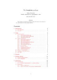
3.6 <strong>The</strong> tdplotsphericalsurfaceplot Command<br />
<strong>The</strong> \tdplotsphericalsurfaceplot command is quite complicated, and it seemed<br />
appropriate to occupy its own section. This command was initially developed<br />
to provide a method of rendering complex polar functions, z = z(θ, φ), where<br />
the magnitude of the function is expressed by the radius, and the phase of the<br />
function is expressed by the hue, as<br />
r = |z(θ, φ)|<br />
hue = Arg [z(θ, φ)]<br />
(3.1)<br />
<strong>The</strong> command has been generalized so that the hue can be specified in terms<br />
of the three polar coordinates, as<br />
r = f(θ, φ)<br />
hue = g(r, θ, φ)<br />
(3.2)<br />
3.6.1 How tdplotsphericalsurfaceplot Works<br />
To achieve the illusion of a 3d surface with proper persistence of vision, the<br />
<strong>tikz</strong>-<strong>3dplot</strong> package divides the drawing task into smaller sections. This<br />
division ensures the surface on the far side of the viewing perspective is properly<br />
occluded from view.<br />
For a given perspective assigned by the main coordinate frame, a “view<br />
orientation” can be defined, giving the angles (θ view , φ view ) that describe the<br />
orientation of the view. <strong>The</strong>se angles determine how to dubdivide the surface<br />
rendering process. <strong>The</strong> following divisions are made:<br />
• Divide the surface into “front” and “back”, where the back is drawn<br />
before the front.<br />
• Subdivide into “left” and “right”.<br />
• Subdivide further into ”top” and ”bottom”.<br />
<strong>The</strong> entire back half is drawn before the front half. For each half, the entire<br />
left or right side is drawn. For each side, all θ angles are drawn in wedges for<br />
each φ angle. When the back half is rendered, the θ angle is swept from θ view<br />
toward the poles. When the front half is rendered, the θ angle is swept from<br />
the poles toward θ view .<br />
During this process, the x, y, and z axes are drawn at the appropriate time,<br />
ensuring the axes are occluded properly by the shape. <strong>The</strong> draw instructions<br />
for these axes are specified as user-defined parameters for this command.<br />
3.6.2 Using tdplotsphericalsurfaceplot<br />
Description: Draws a user-specified spherical polar function, with user-specified<br />
fill hues. Angular range to be displayed is specified with the \tdplotsetpolarplotrange<br />
30
command. <strong>The</strong> line thickness can be specified by issuing the \pgfsetlinewidth<br />
PGF macro.<br />
Syntax: \tdplotsphericalsurfaceplot[fill color style]{theta steps}{phi steps}{function}<br />
{line color}{fill color}{x axis}{y axis}{z axis}<br />
Parameters:<br />
Example:<br />
(Optional) fill color style Specifies whether fill color is a function<br />
of (\tdplotr, \tdplottheta, \tdplotphi), or a direct TikZ color. Set to<br />
parametricfill to enable functional coloring.<br />
theta steps <strong>The</strong> number of steps used to render the surface along the θ<br />
direction. For best results, this number should not be smaller than<br />
12, and should be a factor of 360.<br />
phi steps <strong>The</strong> number of steps used to render the surface along the φ<br />
direction. For best results, this number should not be smaller than<br />
12, and should be a factor of 360.<br />
function A mathematical expression, containing the variables \tdplottheta<br />
and \tdplotphi, used to define the radius of the surface for given angles.<br />
Note that the absolute value of the function is plotted.<br />
line color TikZ color expression for surface lines.<br />
fill color When the option parametricfill is used then this can be some<br />
mathematical expression containing \tdplottheta and \tdplotphi. If<br />
not, then this can be any TikZ expression for color. Note that if the<br />
function specified by function is negative, a shift of 180 is applied<br />
to the color. To avoid this, make sure function is always positive.<br />
x axis Any draw commands used to render the x axis.<br />
y axis Any draw commands used to render the y axis.<br />
z axis Any draw commands used to render the z axis.<br />
\tdplotsetmaincoords{70}{135}<br />
\begin{<strong>tikz</strong>picture}[scale=2,line join=bevel,tdplot_main_coords, fill opacity=.5]<br />
\pgfsetlinewidth{.2pt}<br />
\tdplotsphericalsurfaceplot[parametricfill]{72}{36}%<br />
{sin(\tdplottheta)*cos(\tdplottheta)}{black}{\tdplotphi}%<br />
{\draw[color=black,thick,->] (0,0,0) -- (1,0,0) node[anchor=north east]{$x$};}%<br />
{\draw[color=black,thick,->] (0,0,0) -- (0,1,0) node[anchor=north west]{$y$};}%<br />
{\draw[color=black,thick,->] (0,0,0) -- (0,0,1) node[anchor=south]{$z$};}%<br />
\node[tdplot_screen_coords,fill opacity=1] at (0,-1) {Parametric Fill in $\phi$};<br />
\end{<strong>tikz</strong>picture}<br />
\begin{<strong>tikz</strong>picture}[scale=2,tdplot_main_coords,line join=bevel,fill opacity=.8]<br />
\pgfsetlinewidth{.1pt}<br />
\tdplotsphericalsurfaceplot[parametricfill]{72}{36}%<br />
{0.5*abs(cos(\tdplottheta))}{black}{2*abs(\tdplotr)}%<br />
31
{\draw[color=black,thick,->] (0,0,0)<br />
-- (1,0,0) node[anchor=north east]{$x$};}%<br />
{\draw[color=black,thick,->] (0,0,0)<br />
-- (0,1,0) node[anchor=north west]{$y$};}%<br />
{\draw[color=black,thick,->] (0,0,0)<br />
-- (0,0,1) node[anchor=south]{$z$};}%<br />
\node[tdplot_screen_coords,fill opacity=1] at (0,-1) {Parametric Fill in $r$};<br />
\end{<strong>tikz</strong>picture}<br />
\begin{<strong>tikz</strong>picture}[scale=2,line join=bevel,tdplot_main_coords, fill opacity=.7]<br />
\pgfsetlinewidth{.4pt}<br />
\tdplotsphericalsurfaceplot{72}{24}%<br />
{0.5*cos(\tdplottheta)^2}{black}{red!80!black}%<br />
{\draw[color=black,thick,->] (0,0,0) -- (1,0,0) node[anchor=north east]{$x$};}%<br />
{\draw[color=black,thick,->] (0,0,0) -- (0,1,0) node[anchor=north west]{$y$};}%<br />
{\draw[color=black,thick,->] (0,0,0) -- (0,0,1) node[anchor=south]{$z$};}%<br />
\node[tdplot_screen_coords,fill opacity=1] at (0,-1) {Solid Fill};<br />
\end{<strong>tikz</strong>picture}<br />
z<br />
z<br />
z<br />
x<br />
y<br />
x<br />
y<br />
x<br />
y<br />
Parametric Fill in φ<br />
Parametric Fill in r<br />
Solid Fill<br />
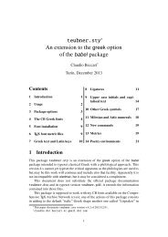
3.6.3 <strong>The</strong> tdplotsetpolarplotrange Command<br />
Description: Defines the range of angles to be displayed when using \tdplotsphericalsurfaceplot<br />
Syntax: \tdplotsetpolarplotrange{lowertheta}{uppertheta}{lowerphi}{upperphi}<br />
Parameters:<br />
lowertheta <strong>The</strong> lower limit for \tdplottheta, in degrees.<br />
uppertheta <strong>The</strong> upper limit for \tdplottheta, in degrees.<br />
lowerphi <strong>The</strong> lower limit for \tdplotphi, in degrees.<br />
upperphi <strong>The</strong> upper limit for \tdplotphi, in degrees.<br />
Example:<br />
32
\tdplotsetmaincoords{60}{110}<br />
\begin{<strong>tikz</strong>picture}[scale=2,line join=bevel,tdplot_main_coords,%<br />
fill opacity=.5]<br />
\tdplotsetpolarplotrange{90}{180}{180}{360}<br />
\tdplotsphericalsurfaceplot[parametricfill]{72}{36}%<br />
{.5}{black}{\tdplotphi + 3*\tdplottheta}%<br />
{\draw[color=black,thick,->] (0,0,0)<br />
-- (1,0,0) node[anchor=north east]{$x$};}%<br />
{\draw[color=black,thick,->] (0,0,0)<br />
-- (0,1,0) node[anchor=north west]{$y$};}%<br />
{\draw[color=black,thick,->] (0,0,0)<br />
-- (0,0,1) node[anchor=south]{$z$};}%<br />
\end{<strong>tikz</strong>picture}<br />
z<br />
x<br />
y<br />
3.6.4 <strong>The</strong> tdplotresetpolarplotrange Command<br />
Description: Resets the range of angles to the default full range when using<br />
\tdplotsphericalsurfaceplot<br />
Syntax: \tdplotresetpolarplotrange<br />
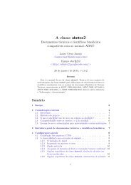
3.6.5 <strong>The</strong> tdplotshowargcolorguide Command<br />
Description: Draws a “color guide” table which associates the hue of a parametric<br />
polar plot with an angle. Guide is drawn at user-specified screen<br />
coordinates with user-specified size. This guide is intended to illustrate<br />
the complex phase representation of the surface for a given θ and φ coordinate.<br />
Syntax: \tdplotshowargcolorguide{x position}{y position}{x size}{y size}<br />
Parameters:<br />
x position <strong>The</strong> x screen coordinate to place the lower-left corner of the<br />
guide.<br />
y position <strong>The</strong> y screen coordinate to place the lower-left corner of the<br />
guide.<br />
x size <strong>The</strong> width of the color guide.<br />
33
y size <strong>The</strong> height of the color guide.<br />
Example:<br />
\tdplotsetmaincoords{40}{0}<br />
\begin{<strong>tikz</strong>picture}[scale=2,line join=bevel,tdplot_main_coords,%<br />
fill opacity=1]<br />
\tdplotsphericalsurfaceplot[parametricfill]{72}{36}%<br />
{sqrt(15/2)/2*sin(\tdplottheta)^2}{black}%<br />
{2*\tdplotphi - 6 * \tdplottheta}{}{}{}%<br />
\tdplotshowargcolorguide{3}{-.2}{.1}{1}<br />
\end{<strong>tikz</strong>picture}<br />
2π<br />
π<br />
0<br />
3.7 Miscellaneous Math Commands<br />
<strong>The</strong> following commands are used to streamline the <strong>tikz</strong>-<strong>3dplot</strong> calculations<br />
in the background. <strong>The</strong>re is generally no need to use these directly, but may<br />
be useful on their own for any desired calculations.<br />
3.7.1 tdplotsinandcos<br />
Description: Determines the sine and cosine of the specified angle, and stores<br />
in specified macros.<br />
Syntax: \tdplotsinandcos{sintheta}{costeta}{theta}<br />
Parameters:<br />
sintheta A macro (eg. \sintheta) to store the sine of theta.<br />
costheta A macro (eg. \costheta) to store the cosine of theta.<br />
theta An angle (in degrees) to calculate. Can be a macro or literal value.<br />
34
3.7.2 tdplotmult<br />
Description: Determines the product of two specified values, and stores the<br />
result in the specified macro.<br />
Syntax: \tdplotmult{result}{multiplicand}{multiplicator}<br />
Parameters:<br />
result A macro (eg. \result) to store the product of multiplicand *<br />
multiplicator.<br />
multiplicand <strong>The</strong> multiplicand of the product.<br />
literal value.<br />
Can be a macro or<br />
multiplicator <strong>The</strong> multiplicator of the product. Can be a macro or<br />
literal value.<br />
3.7.3 tdplotdiv<br />
Description: Determines the quotient of two specified values, and stores the<br />
result in the specified macro.<br />
Syntax: \tdplotdiv{result}{dividend}{divisor}<br />
Parameters:<br />
result A macro (eg. \result) to store the quotient of dividend /<br />
divisor.<br />
dividend <strong>The</strong> dividend of the quotient. Can be a macro or literal value.<br />
divisor <strong>The</strong> divisor of the quotient. Can be a macro or literal value.<br />
35
Chapter 4<br />
Known Issues<br />
<strong>The</strong>re are various issues that have been found while developing the <strong>tikz</strong>-<strong>3dplot</strong><br />
package. Some of these are currently open problems which will hopefully be<br />
resolved. Feedback and suggestions are welcome.<br />
4.1 Predefined Points Don’t Work in Rotated Frame<br />
When a coordinate is defined using the TikZ command \coordinate, it will be<br />
transformed by the transformation specified at the beginning of the <strong>tikz</strong>picture<br />
environment. <strong>The</strong>se coordinates will not work for transformations applied at<br />
the actual \draw command.<br />
This problem seems to be inherant with TikZ itself. By way of example,<br />
the following code is taken right from the PGF manual Version 2.00, section<br />
21.2 on page 218:<br />
Case A:<br />
%this one works fine using literal coordinates<br />
\begin{<strong>tikz</strong>picture}[smooth]<br />
\draw plot coordinates{(1,0)(2,0.5)(3,0)(3,1)};<br />
\draw[x={(0cm,1cm)},y={(1cm,0cm)},color=red]<br />
plot coordinates{(1,0)(2,0.5)(3,0)(3,1)};<br />
\end{<strong>tikz</strong>picture}<br />
Two distinct paths shown.<br />
All is good.<br />
Case B:<br />
%this one does not work using predefined coordinates<br />
\begin{<strong>tikz</strong>picture}[smooth]<br />
\coordinate (A) at (1,0);<br />
\coordinate (B) at (2,0.5);<br />
\coordinate (C) at (3,0);<br />
\coordinate (D) at (3,1);<br />
\draw plot coordinates{(A)(B)(C)(D)};<br />
\draw[x={(0cm,1cm)},y={(1cm,0cm)},color=red] plot coordinates{(A)(B)(C)(D)};<br />
36
\end{<strong>tikz</strong>picture}<br />
Both paths draw overtop each other, and the coordinates are not transformed!<br />
Case A:<br />
Two distinct paths shown. All is good.<br />
Case B:<br />
Both paths draw overtop each other, and the coordinates are not transformed!<br />
4.2 node Command and shift=(P) Issues<br />
When placing a node in a shifted coordinate frame, the \node command will<br />
not position properly. As a workaround, the \draw command must be used to<br />
position the node. By way of example.<br />
Case A:<br />
\tdplotsetmaincoords{60}{110}<br />
\begin{<strong>tikz</strong>picture}[scale=3,tdplot_main_coords]<br />
\draw[thick,->] (0,0,0) -- (1,0,0) node[anchor=north]{$x$};<br />
\draw[thick,->] (0,0,0) -- (0,1,0) node[anchor=west]{$y$};<br />
\draw[thick,->] (0,0,0) -- (0,0,1) node[anchor=south]{$z$};<br />
\coordinate (P) at (3,3,3);<br />
\tdplotsetrotatedcoords{0}{0}{0}<br />
\tdplotsetrotatedcoordsorigin{(P)}<br />
\draw[thick,tdplot_rotated_coords,->] (0,0,0)<br />
-- (.5,0,0) node[anchor=north]{$x’$};<br />
\draw[thick,tdplot_rotated_coords,->] (0,0,0)<br />
-- (0,.5,0) node[anchor=south west]{$y’$};<br />
\draw[thick,tdplot_rotated_coords,->] (0,0,0)<br />
-- (0,0,.5) node[anchor=south east]{$z’$};<br />
\node[tdplot_rotated_coords] at (30:.5){$\theta_{bad}$};<br />
\draw[tdplot_rotated_coords] (0,0,0) + (30:.5) node{$\theta_{good}$};<br />
\end{<strong>tikz</strong>picture}<br />
37
Here, the rotated coordinate frame is shifted by amount (P) within the main%<br />
coordinate frame. <strong>The</strong> node labelled $\theta_{bad}$ does not accept any%<br />
positioning coordinates.<br />
Case B:<br />
\tdplotsetmaincoords{60}{110}<br />
\begin{<strong>tikz</strong>picture}[scale=3,tdplot_main_coords]<br />
\draw[thick,->] (0,0,0) -- (1,0,0) node[anchor=north]{$x$};<br />
\draw[thick,->] (0,0,0) -- (0,1,0) node[anchor=west]{$y$};<br />
\draw[thick,->] (0,0,0) -- (0,0,1) node[anchor=south]{$z$};<br />
% \coordinate (P) at (3,3,3);<br />
\tdplotsetrotatedcoords{0}{0}{0}<br />
% \tdplotsetrotatedcoordsorigin{(P)}<br />
\draw[thick,tdplot_rotated_coords,->] (0,0,0)<br />
-- (.5,0,0) node[anchor=north]{$x’$};<br />
\draw[thick,tdplot_rotated_coords,->] (0,0,0)<br />
-- (0,.5,0) node[anchor=south west]{$y’$};<br />
\draw[thick,tdplot_rotated_coords,->] (0,0,0)<br />
-- (0,0,.5) node[anchor=south east]{$z’$};<br />
\node[tdplot_rotated_coords] at (30:.5){$\theta_{bad}$};<br />
\draw[tdplot_rotated_coords] (0,0,0) + (30:.5) node{$\theta_{good}$};<br />
\end{<strong>tikz</strong>picture}<br />
Here, the shift is removed from the rotated coordinate frame. <strong>The</strong> %<br />
previously failing \verb|\node| command works properly.<br />
z ′<br />
z<br />
θ y ′<br />
bad<br />
θ<br />
x ′ good<br />
y<br />
Case A:<br />
x<br />
Here, the rotated coordinate frame is shifted by amount (P) within the<br />
main coordinate frame. <strong>The</strong> node labelled θ bad does not accept any positioning<br />
coordinates.<br />
38
z<br />
z ′ θ bad<br />
y ′<br />
θ<br />
x ′ good<br />
Case B: x<br />
Here, the shift is removed from the rotated coordinate frame. <strong>The</strong> previously<br />
failing \node command works properly.<br />
y<br />
4.3 PGF xyz spherical Coordinate System<br />
I have recently heard about the xyz spherical coordinate system offered by<br />
PGF. Unfortunately, when I try to use it, I get compile errors. I haven’t spent<br />
much time looking into it though, so I’m probably just doing something silly.<br />
\draw[-stealth,color=orange] (0,0,0)<br />
-- (xyz spherical cs:radius=.5,longitude=60,latitude=120);<br />
%this gives the following compile error using MikTeX 2.8:<br />
% Undefined control sequence. \<strong>tikz</strong>@cs@radius.<br />
39
Chapter 5<br />
TODO list<br />
This chapter contains notes and jots of ideas of things to do which can expand<br />
or improve the <strong>tikz</strong>-<strong>3dplot</strong>package.<br />
• Figure out how to work in a variable scope that doesn’t interfere with<br />
other packages.<br />
• Find a way to check if TikZ is loaded, and give a compile error if necessary.<br />
• Find a way to use predefined coordinates in rotated or translated coordinate<br />
frames, instead of just literal coordinates.<br />
• Generalize matrix math if such a package exists.<br />
• Look into using TikZ spherical polar coordinates explicitly to streamline<br />
coordinate definitions.<br />
• Find a way to extract coordinate components defined by the \coordinate<br />
command and use them in macros defined by the \pgfmathsetmacro and<br />
\pgfmathparse commands.<br />
40