download

Direct Measurement of the Turbulent Kinetic Energy Viscous
Dissipation Rate Behind a Grid and a Circular Cylinder
A. Ducci, E. Konstantinidis, S. Balabani and M. Yianneskis
Experimental and Computational Laboratory for the Analysis of Turbulence (ECLAT)
Department of Mechanical Engineering, King’s College London
Strand, London WC2R 2LS, United Kingdom
Abstract
A method is presented to evaluate the turbulent kinetic energy viscous dissipation rate, ε, from the direct
measurement of the mean squared turbulent velocity spatial gradients
( ∂ u ∂
2
/ x )
i j
. The latter have been
estimated using Laser Doppler Anemometer to measure simultaneously the velocities in two different points in
the flow. To minimise the effect of virtual particle bias and of geometry bias the control volume dimensions
have been reduced collecting the light in side scatter and using short focal length lenses. The methodology has
been tested in the isotropic and homogeneous region of a turbulent flow downstream of a grid where ε is
proportional to the kinetic energy decay. The measurements were carried out in a water rig for a Reynolds
number Re M of 5500, based on a mesh size M (5.5 mm) of the grid, along the centreline in a range between 23-
35 M. Isotropic and homogenous conditions were satisfactorily achieved. In agreement with theory, the
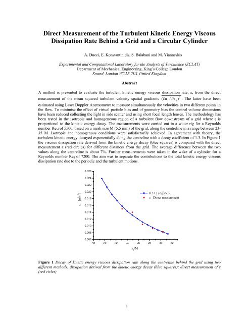
turbulent kinetic energy decayed exponentially along the centreline with a decay coefficient of 1.3. In Figure 1
the viscous dissipation rate derived from the kinetic energy decay (blue squares) is compared with the direct
measurement ε (red circles) for different distances from the grid. The average difference between the two
values along the centreline is about 7%. Further measurements were taken in the wake of a cylinder for a
Reynolds number Re d of 7200. The aim was to separate the contributions to the total kinetic energy viscous
dissipation rate due to the periodic and the turbulent motions.
0.026
0.024
0.022
ε [m 2 s -3 ]
0.020
0.018
0.016
0.014
0.012
0.010
0.008
0.5 U 1
(∂q 2 /∂x 1
)
ε Direct measurement
0.006
18 20 22 24 26 28 30 32
x 1
/M
Figure 1 Decay of kinetic energy viscous dissipation rate along the centreline behind the grid using two
different methods: dissipation derived from the kinetic energy decay (blue squares); direct measurement of ε
(red cirles)
1

1. Introduction
The knowledge of the rate of dissipation of turbulence kinetic energy per unit mass, ε, is of great importance in
fluid mechanics, e.g. many turbulence models include an equation for ε and therefore is essential for testing the
applicability of the models commonly used. However its accurate experimental determination poses a challenging
problem. The rate of dissipation of turbulence kinetic energy is defined as follows Hinze (1975):
⎛
⎜
∂u
⎝ ∂x
i j j
ε = ν +
(1)
j
∂u
⎞ ∂u
⎟
∂x
i ⎠ ∂x
i
These limitations are usually overcome assuming, even for more complex flows, local isotropy, simplifying
equation (1) as follows:
2
⎛ ∂u
⎞
1
ε = 15 ν ⎜ ⎟
(2)
⎜ x ⎟
⎝ ∂
1 ⎠
As pointed out by Elsner & Elsner (1996), with this hypothesis the different terms comprising the dissipation
equation are related as follows:
K
ijij
K
2
2
⎛ ∂u
⎞
j ⎛ ∂u
⎞
1
= ⎜ ⎟
1
x
⎜
j
x
⎟
(3)
⎝ ∂ ⎠ ⎝ ∂
1 ⎠
jj
=
2
2
⎛ u ⎞ ⎛ u ⎞
⎜
∂
i
∂
1
= ⎟ = 2 for i ≠ j
x
⎜
x
⎟
(4)
⎝ ∂
j ⎠ ⎝ ∂
1 ⎠
2
⎛ u ⎞ ⎛ ∂u
j ⎞ ⎛ u ⎞
1
1
K ⎜
∂
i
∂
= ⎟
= − for i ≠ j
ijji
x
⎜
j
x
⎟
⎜
i
x
⎟
(5)
⎝ ∂ ⎠ ⎝ ∂ ⎠ ⎝ ∂
1 ⎠ 2
The assumption of homogeneous turbulence is less restrictive than that of isotropic turbulence and assuming
symmetric flow (u 2 = u 3 ) and symmetric geometry ( ∂ ∂x
2
= ∂ ∂x
3
), equation (1) becomes:
⎡
2
2
2
2
2
⎤
⎢
⎛ ∂u
⎞ ⎛ ∂u
⎞ ⎛ ⎞ ⎛ ∂ ⎞ ⎛ ∂ ⎞
3
∂u
u u
1
1
3
3
ε = ν
+ + + ⎥
⎢
⎜
⎟ + 2
⎜
⎟ 2
⎜
⎟ 2
⎜
⎟ 2
⎜
⎟
(6)
⎥
⎣
⎝ ∂x
⎠ ⎝ ∂x
⎠ ⎝ ∂x
⎠ ⎝ ∂x
⎠ ⎝ ∂x
1
3
3
1
2 ⎠
⎦
In the published literature, (e.g. Tennekes & Lumley (1973)), nearly homogeneous and isotropic flow is usually
assumed to be reached behind a grid, where the wakes created by the rods merge together, after an initial region of
high inhomogeneity and anisotropy. As described by Tennekes & Lumley (1973), in the homogeneous and
isotropic region the equation for the turbulence mean kinetic energy can be simplified as follows:
⎛
2
U ⎞
1
⎜
∂q
⎟ = − ε
(7)
2
⎝
∂x
1 ⎠
The rate of change of the kinetic energy in time (the convective term) is equal to the viscous dissipation, so that
2
q decays constantly along the axis X 1 of the main flow, following a relationship of the form:
u
2
−n
⎛ x x
0 ⎞
= A ⎜ − ⎟
2
(8)
U ⎝ M M ⎠
1
where M is the mesh spacing, n is the exponent characterising the decay of turbulence, x is the distance from the
grid, and x 0 is a virtual origin which accounts for the fact that the effective origin of the velocity fluctuations may
not coincide with the location of the grid.
In the earliest study of grid generated turbulence, referred to in Comte-Bellot & Corssin (1966), the values of n and
x 0 /M varied respectively from 1 - 1.3 and 0 - 10, depending on the initial conditions such as mesh size M, rod shape
(parallelepipedal or cylindrical), solidity ratio σ, and mesh Reynolds number Re M .
There have been many studies of grid turbulence since this seminal work of Comte-Bellot & Corssin (1966). The
description of the flow has, in general, improved with the accuracy of the measurement techniques and for this
reason only the most recent relevant works are considered below.
2

Mohamed & LaRue (1990) performed an extensive study of this flow in a wind tunnel and reviewed some of the
earliest works. They emphasised that using only data belonging to the homogeneous isotropic region, n and x 0 /M
do not depend on the initial conditions and assume values around 1.30 and 0 respectively. They suggested different
methods to determine the beginning of the isotropic region: the skewness of the velocity fluctuation S(u) and of the
velocity derivative S(du/dx) should be equal to 0 and to a constant respectively, and the ratio between the
dissipation calculated with equation (7), for grid turbulence flow, and with the equation (2), for local isotropic
flow, should be 1 for the entire homogeneous and isotropic region. As Re M was decreased, the start of the
homogeneous area was found to be located closer to the grid.
In addition to the method used by Mohamed & LaRue (1990), Tresso & Munoz (2000) determined also the
beginning of the isotropic and homogenous region for different initial conditions, by applying directly the
definition of isotropy ( u1 u
2
= 0 ). Using this approach they determined an experimental law describing the
beginning of the isotropic and homogeneous region as a function of Re M .
In agreement with Mohamed & LaRue (1990), Zhou et al. (2000), measuring at a distance x/M higher than 20,
obtained an exponent n equal to 1.33 and a value of x 0 equal to 0.
The flow conditions and the main results of the aforementioned works are summarised in Table 1:
Table 1. The decay power-law exponent (n), coefficient (A) and other parameters in previously published
works.
Beginning of
Ref. Re M x 10 -3 Fluid Isotropic
Hom. Region
n A x 0 /M σ M/d
Comte-
Bellot &
Corssin
(1966)
Mohamed &
LaRue
(1990)
Zhou et al
(2000]
135-17 Air 20 * 1.1-
1.33
0.05 3-5
0.31-
0.44
6 " 25 1.30 0.0435 0 0.34 5.4
10 " 40 1.30 0.0424 0 " 5.4
14 " 50 1.28 0.0364 0 " 5.4
12 " 55 1.29 0.0490 0 " 5.3
10.5 " 30 * 1.33 - 0 0.35 5.2
Tresso & 10.7 18
Munoz 22.9 "
28
- - - 0.28 8
[2000] 34
57
* These works did not evaluate the coordinate x/M where the flow becomes isotropic and homogeneous. This
value identifies the distance from the grid where the first measurements were made.
(-) This symbol means that the parameter is not available
Direct measurement of the spatial gradients using a two channel LDA was attempted by Michelet (1998) in grid
turbulence flow. Because of the difficulty encountered in measuring the decay of the kinetic energy (n=0.33),
Michelet (1998) compared the values of the dissipation using equation (6) for homogeneous flow and equation (2)
for local isotropic turbulence. The latter was computed by integrating the energy spectrum of the velocity
fluctuations. The agreement obtained was excellent, but the expressions of the equations applied leave some doubt
as to the validity of the results.
Another work which attempted to calculate directly the spatial gradients, has been reported by Benedict & Gould
(1996). The intention of that work was to calculate the gradients by estimating the Taylor micro scale from the
spatial correlation coefficients R ii (∆x j ) and R ii (∆x i ) in sudden contraction flow. They pointed out how the
dimensions of the control volumes affect the accuracy of the determination of the spatial correlation coefficient, as
a control volume which is too large gives a poor resolution of R ii (∆x j ). They suggested that for a proper estimation
of R ii (∆x j ) the control volume should be of the order of the Kolgomorov scale.
-
3

Apart from the necessity to have an isotropic and homogeneous flow, it is necessary to discuss the errors involved
in multidimensional LDA measurement. Three types of bias are relevant in such systems.
Boutier et al (1985) considered the possibility that in 3-D LDA measurements two different particles could satisfy
a simultaneity criterion, crossing the control volumes within a defined time interval, even if they would not pass
through the overlapping region. This results in a source of error, termed virtual particle bias, which leads to a
substantial underestimation of the Reynolds stresses.
The second type of bias, the geometry bias, was firstly determined by Brown (1989); he established that even a
single particle, with a consistent velocity component in the plane containing the axis of the two control volumes,
could pass outside the overlapping region within the time coincidence window.
The effect of the third type of bias, the time coincidence bias, was determined by Benedict & Gould (1996) during
their study of the spatial correlation coefficient. When the two control volumes are separated by a small distance
along the direction of the dominant velocity of the flow, it is possible that a single particle will cross both the
control volumes within the time coincidence window, resulting in an overestimation of the correlation coefficient.
2. Flow configuration, LDA system and measurement procedure
The rig consists of a single loop pipe arrangement with a by-pass and a centrifugal pump, which directs the water
into an expansion/contraction section containing a hexagonal honeycomb to straighten the flow. A perforated plate
is placed downstream the contraction to reduce the turbulence levels before the flow reaches the grid. The
measurements are taken in the second half of a transparent acrylic test section to allow the flow to become
homogeneous and isotropic. A heat exchanger jacket in a tank downstream of the test section maintains the
temperature of the water at a constant value. The dimensions of the grid and of the test section used are shown in
following Table 2:
Table 2. Test section and grid dimensions
Test section dimensions
Grid
(W x W x L) Mesh size (M) Wire diameter (D)
72 x 72 x 184 mm 3 5.5 mm 1 mm
The LDA employed is a Dantec system and comprises three probes mounted on a transverse that can be remotely
moved in all the directions. One of the probes can measure two velocity components while the others can measure
only one. The probes are designed to work in the back-scatter mode.
The arrangements of the probes for the measurements of the gradients
2
( ∂ u x ) , ( ∂ u ∂ ) 2
, ( ∂ u ∂ ) 2
, ( ∂u
∂ ) 2
1
∂
1
1
x 3
3
x 3
3
x 1
are shown in Figure 2. The two-channel probe shown in blue is
displaced along the directions indicated. Depending on the gradient of interest, the green probe measures the u 1
velocity (Figure 2.(a)) or the u 3 velocity (Figure 2.(b)). The blue and green probes incorporate lenses of focal length
240 mm and of 310 mm respectively. The control volume dimensions for the lenses mounted on the three probes
are shown in Table 3.
To reduce the longer dimension of the green control volume the light scattered by the 10 µm diameter particles is
collected in side scatter by the red probe. The red probe incorporated a lens of focal lens 310 mm or 500 mm
depending on the arrangement (Figure 2 (a) or (b) respectively) to ensure that all three lenses focused at the same
point.
Accurate calculation of the effective size of the control volume in side scatter is not possible because, even if the
diameter of the fibre optic cable (50 µm), substituting in this system the pinhole usually placed in front of the
photomultiplier, is known, the exact lens magnifying power is unknown. From geometry considerations, taking in
to account that the angle between the optical axes of the side probes and of the centre probe is about 22°, the longer
dimension of the green control volume for side scatter should be around 0.24 mm.
4

Table 3. Focal length and control volume dimensions, in back scatter, of the lenses employed
Probe Focal length Diameter dx1 Diameter dx2 Length dx3
Blue Probe 240 mm 0.05 mm 0.05 mm 0.37 mm
Green probe 310 mm 0.07 mm 0.07 mm 0.63 mm
Red Probe
310 mm 0.07 mm 0.07 mm 0.63 mm
500 mm 0.125 mm 0.124 mm 1.7 mm
X 3
X 2
X 1
X 2
X 3 X 1
(a)
(b)
2
Figure 2 Probe arrangement to measure the velocity gradients: (a) ( ∂ u x ) , ( ∂ u ∂ ) 2
; (b) ( u ∂ ) 2
( u ∂ ) 2
∂ .
3
x 1
1
∂
1
1
x 3
∂ ,
3
x 3
The probes are aligned in air using a pinhole of 50 µm. Once in water, to overcome the effect of refraction, it is
necessary to adjust the relative position of the three control volumes along the X 2 axis by a known distance. As
suggested by Benedict & Gould (1996) a further optimisation of the alignment is achieved computing the spatial
correlation coefficient R ii (0) for different relative positions of the probes until a maximum is found.
The spatial gradients ( u ∂ ) 2
∂ are estimated calculating the function f ii (∆x j ) defined in (9) for the different
i
x j
positions examined around the reference point x i :
f
2
( x ) = (u (x , t) − u (x + ∆x
, t))
ii j
i j
i j j
∆ (9)
When computing the coefficient f ij (∆x j ), the velocity fluctuations u i in the two different points of measurement
must come from particles which cross the two control volumes at the same time. This condition is imposed by
finding the couples of particles that satisfy the following simultaneity criterion:
|t 1 -t 2 | < τ w , (10)
where t 1 and t 2 are the arrival time and τ w is a time coincidence window.
Once the function f ij (∆x j ) is known, the spatial gradient can be calculated from (11)
2
( u ( x , t) − u ( x + ∆x
, t
)
2
⎛ u ⎞
i j
i j j
⎜
∂
i
⎟ = lim
(11)
x 0
2
j
x
∆ ⇒
⎝ ∂
j ⎠
∆x
j
The spatial gradient can be evaluated by finding the slope of the straight line which best fits the points (∆x 2 j ,
f ii (∆x j )) for ∆x j values close to zero. Once all the gradients have been determined, the value obtained for the
dissipation rate estimated from equation (6) for homogenous flow is compared with the value obtained from
equation (7) for grid turbulence flow.
5

3. Grid turbulence flow
The experiments were carried out along the centreline of the test section for a mesh Reynolds number Re M of 5500.
2
2
Figure 3 shows the rate of decay of the kinetic energy and of the turbulence intensities u1 U1
and u
3
/ U
1
along the X 1 direction. It is evident that the flow is not perfectly isotropic as the turbulence intensities along axis X 1
and X 3 are not the same. This difference was also present in previous works, such as Comte-Bellot & Corssin
(1966) and Zhou et al. (2000) and wasn’t considered to be significant, as the difference between the rms values in
the two directions is within the accuracy of the LDA system.
2
2
0.01
u i
2
/U1
2
u 1 2 /U 1
2
u 3 2 /U 1
2
1E-3
q 2 /U 1
2
Linear fit
10 20 30 40 50
X 1
/M
Figure 3 Decay of q
2
U
1
2
2
, u
1
U1
and u
2
2 2
3
/ U1
along the duct centre line
As suggested by Mohamed and Larue (1990), the coefficients of the exponential law shown in (8) have been
estimated applying a least-squares linear regression between points belonging to the homogenous and isotropic
region. This is found to begin at a distance of 20 M from the grid. Considering that Mohamed & Larue (1990)
determined that the beginning of the isotropic and homogeneous region is closer to the grid as Re M is decreased,
this value should be considered in good agreement with the others shown in Table 1. The decaying coefficients n
2
found for q U 2 2
, u U 2
2
2
and u / are 1.31, 1.27 and 1.35 respectively.
1
1
1
3
U
1
4. Rate of dissipation for the grid turbulence flow
The direct measurement of the spatial gradients has been carried out between 20 and 35 M for a Re M of 5500.
In Figure 4 the values assumed by f ii (∆x j ) at a distance of 23 M from grid, are plotted against ∆x j 2 for all the
gradients measured. The time coincidence windows τ w applied is of 0.03 ms. All the f ii (∆x j ) have been evaluated
for distances ∆x j between 0-0.7 mm with a step of 0.1 mm.
Considering Figure 4, it can be observed that the values of f ii (∆x i ) for ∆x j 2 > 0 are much higher than for f 11 (0). This
substantial difference has to be attributed to the relatively large dimensions of the control volume. On the one hand,
when the probes are displaced, it is very unlikely that two particles will cross the centre of the two control volumes
at the same time to give a highly correlated pair of velocity values. It is more probable that one of them will pass
through the centre of one control volume while the other will pass far away from the centre of the second control
volume, resulting in a higher distance between the points where the control volumes are crossed than the effective
displacement ∆x j effectuated. This leads to velocity pairs less correlated than expected. On the other hand, when
6

the two probes are aligned at the same point, each particle crossing one control volume will more likely cross the
second control volume in the same point giving always highly correlated velocity pairs.
12
Position: x 1
=110 mm; x 1
/M=23.09
Position: x 1
=110 mm; x 1
/M=23.09
(u 3
(x+∆x)-u 3
(x)) 2 [cm 2 s -2 ]
10
8
6
4
2
(∆u 3
(∆x 1
)) 2
(∆u 3
(∆x 3
)) 2
Linear fit: slope = (∂u 3
/∂x 1
) 2
(u 1
(x+∆x)-u 1
(x)) 2 [cm 2 s -2 ]
15
10
5
(∆u 1
(∆x 1
)) 2
(∆u 1
(∆x 3
)) 2
Linear fit: slope = (∂u 1
/∂x 1
) 2
Linear fit: slope = (∂u 1
/∂x 3
) 2
0
0.0 0.3 0.6 0.9 1.2 1.5
∆x 2 [mm 2 ]
Linear fit: slope = (∂u 3
/∂x 3
) 2 a)
0
0.0 0.3 0.6 0.9 1.2 1.5
∆x 2 [mm 2 ]
b)
Figure 4 Variation of f ii (∆x j ) with ∆x 2 j in x 1 /M=23.09: (a) ( ∂ u ∂ ) 2
, ( ∂ u ∂ ) 2
2
; (b) ( ∂ u x ) , ( u ∂ ) 2
R 33
(∆x j
)
3
x 3
3
x 1
1
∂
1
∂ .
The same effect is evident also in Figure 5 where the variation of the spatial correlation factors R 33 (∆x 3 ) and
R 33 (∆x 1 ) is plotted against ∆x j . The value of R 33 (∆x j ) for ∆x j equal to zero is much higher than those for ∆x j
different than zero. For this reason the (0, f ii (0)) pairs have not been considered in the line fitting to determine the
spatial gradient values.
As can be seen in Figure 4 the value of R 33 (0) is 0.92
and far from the ideal correlation coefficient that
0.9
should be 1 for ∆x j equal to zero. There are three main
0.8
R 33
(∆x 3
) reasons to explain this difference. The first one has to
R 33
(∆x 1
)
be attributed to the size of the control volume which,
Parabola fitting
0.7
despite the small dimension, is still too big for a
perfect correlation. The second one is due to the noise
0.6
level. In fact the necessity to have a sufficient amount
of data in coincidence between the two channels leads
0.5
to use higher values of the High Voltage (HV). This
0.4
was confirmed through trials with a decreasing HV,
for which the correlation reached a maximum value of
0.3
0.96. The third, probably the most important, has to be
-1.5 -1.0 -0.5 0.0 0.5 1.0 1.5
∆x j
[mm]
attributed to the flow and the limits of the BSA. In fact
the turbulence level is very small so that the
correlation and the f ii value depends mostly on the
Figure 5 Correlation factors R 33 (∆x 3 ) and R 33 (∆x 1 ) in second decimal digit of the velocity fluctuation value.
x 1 /M of 23.09
This problem is more visible if the light scattered by
the same control volume is collected from two
different probes, one in back scatter and one in side
scatter. Despite the velocities measured belonging for certain to the same particles, the correlation value is 0.96.
Therefore this value has to be considered as the intrinsic error of the system.
The perfect symmetry of the two correlation functions represent in Figure 4 is artificial and not experimental. To
plot the parabola best fitting the points illustrated in Figure 4, R 33 (-∆x j ) has been set equal to R 33 (∆x j ). Considering
in Figure 4 the fitted lines for the four different spatial gradients, it is possible to appreciate qualitatively how the
slopes of the gradients ( ∂u
∂ ) 2
and ( ∂u
∂ ) 2
are higher and around twice the slopes of ( ∂u
∂ ) 2
( ∂u
∂ ) 2
1
x 3
3
x 1
1
x 1
1
x 3
and of
3
x 3
respectively. This is visible also in Figure 5 where the parabola fitted between the R 33 (∆x 1 ) values is
narrower than that fitted in R 33 (∆x 3 ). The variation of the spatial gradients
7

( ∂ u ∂ ) 2
, ( ∂ u ∂ ) 2
, ( ∂ u ∂ ) 2
, ( ∂u ∂ ) 2
1
x 1
3
x 1
1
x 3
3
x 3
along the duct centreline is plotted in Figure 6. The gradients
have been evaluated by fitting a line between the values of f ii (∆x j ) for ∆x j varying between 0.1-0.6 mm. This
corresponds to a range of 1-5 Kolgomorov scale η. The best fitting line has been found maximising the correlation
factor R of the linear interpolation. Regardless of the experimental scatter of the gradient values, the isotropic
conditions illustrated in equations (3), (4) are satisfactorily achieved.
(∂u/∂x) 2 [ s -2 ]
2200
2000
1800
1600
1400
1200
1000
800
600
400
0.5 U 1
(∂q 2 /∂x 1
)(1/15 ν)
(∂u 1
/∂x 1
) 2
(∂u 1
/∂x 3
) 2
(∂u 3
/∂x 3
) 2
(∂u 3
/∂x 1
) 2
(1/U 2 1
)(∂u 1
/∂t) 2
200
18 20 22 24 26 28 30 32 34 36 38
x 1
/M
Figure 6 Comparison between the values assumed by the spatial gradients directly measured (red, black, blue and
green circles) and the ( ∂u
∂ ) 2
hypothesis (triangles).
1
x 1
gradient calculated from the kinetic energy decay (violet line) and from Taylor's
In Figure 6 the values of the spatial gradients measured directly are compared with the values of
( ∂u
∂ ) 2
1
x 1
calculated with the kinetic energy decay and with Taylor hypothesis. The latter gradients have been
calculated applying the slotting technique (Van Maanen & Tummers (1996)), normally used to determine the
autocorrelation coefficient. In the present work the technique is used to evaluate the f ii coefficients for different
time intervals ∆t. Even in this case the time coincidence window used is 0.03 ms. The different methods
implemented show a good agreement.
A comparison between the values of the scaled dissipation ( ε M/ U 1
) from the present and previous works is
shown in Figure 7. The dissipation values are calculated from the kinetic energy decay. The coefficients A and n of
the kinetic energy decay have been taken from Mohamed & LaRue (1990) who, as already mentioned, revisited
some of the earliest work on grid turbulence flow. The non dimensional dissipation values have been plotted for
X 1 /M in the range of 20-40 M. The values of ε M/ U 1
shown in Figure 7 differ by a large amount (46 %
difference between the values of the curves located furthest away from each other).
Considering the high values of Re M used in some of the past works, it is possible that for some of them the
isotropic region commenced somewhere in the range or even at higher distances from the grid, but this do not
affect the validity of the graph. In fact the dissipation decaying coefficients (1+n) of the curves plotted vary by
small amounts (2.26-2.35), so that can be assumed that all the curves remain parallel to each other and their
differences do not become smaller for higher values of x 1 /M. The high difference between the scaled values
3
ε M/ U 1
is due to the substantial variation of A (0.0364-0.0664) from one work to the other. From Figure 7 it can
3
be observed that the values of ε M/ U 1
of the present work lie between the curves of the previous works.
3
3
8

ε M/ U 1 3
1E-4
Larue Re M
= 6000
" Re M
= 10000
" Re M
= 14000
" Re M
= 12000
Wyatt(1955) Re M
= 11000
Van Atta & Chen (1969) Re M
= 25600
Comte-Bellot & Corsin (1966) Re M
= 34000
Sreenivasan et al. (1980) Re M
= 7400
Uberoi (1963) Re M
= 10000
Uberoi & Wallis (1967) Re M
=29000
Sirivat & Warhaft (1983) Re M
=8750
present data Re M
=5150
1E-5
20 25 30 35 40 45 50 55 60
x 1
/M
Figure 7 Comparison between the values assumed by the dimensionless dissipation
previous works.
ε M/ U 1
3
in the present and in
The comparison between the values of the dissipation calculated from the decay of kinetic energy and from the
direct estimation of the gradients have been illustrated in Figure 1. According to the isotropic relation (4), the
contribution to dissipation due to the spatial gradient ( u ∂ ) 2
gradients ( ∂ u ∂ ) 2
and ( u ∂ ) 2
1
x 3
∂ .
3
x 1
5. Flow in the wake of a cylinder
∂ in (6) have been substituted with the spatial
3
x 2
X 1 /d
X 1
X 3
The measurements were carried out across the wake of the
cylinder along a line parallel to the X 3 direction located in the
centre of the test section and at a distance from the cylinder of
X 1 /d equal to 10 (Figure 8). The points of measurements are
X 3 /d: -0.2, -0.1, 0, 0.1, 0.2, 0.3, 0.4, 0.5, 0.8, 1.2, 1.6, 2.
The Reynolds number Re d is 7200 and the diameter d of the
cylinder is 7.2 mm.
Line of
measurement
X 2
X 3
Figure 8 Diagram showing the locations where
the measurements were taken
The method used to determine the gradients is the same as
described earlier for the grid turbulence flow. In this case it is
necessary to separate the turbulence from the periodic motions
due to the presence of mean flow variations due to vortex
shedding. As for the grid turbulence flow, the two data series,
one from each of the two probes, have been scanned to find
the particles that satisfy the condition of equation (10).
The periodic motions have been identified by low pass
filtering the spectra of the two data series.
In Figure 9 the total velocities of the particles in coincidence
and the velocities due to the periodicity of the flow (the low
pass filtered velocities) are shown.
9

0.6
u [m s -1 ]
0.4
0.2
0.0
ub periodic
(low pass filtered velocity)
ug periodic
" "
ub tot
(velocity in coincidence)
ug tot
" "
-0.2
-0.4
-0.6
31.0 31.1 31.2 31.3
Time [s]
Figure 9 Comparison between the values of the low pass filtered velocity and the total velocity of the particles in
coincidence for each channel (blue and green).
Considering that the frequency of the periodical motion is 30 Hz, the data have been low pass filtered up to a
frequency of 50 Hz. The turbulent velocities have been calculated by subtracting the periodic velocity from the
total velocity of the particles in coincidence. The variations of the spatial gradients values against X 3 /d are shown
in Figure10. The gradients have been calculated by determining the slopes of the lines providing the best fit of the
pairs (∆x j, f ii (∆x j ) for ∆x j varying between 0.1-0.3 mm.
500
(∂u 3
/∂x 1
) 2 [s -2 10 -2 ]
400
300
200
(∂u 1
/∂x 1
) 2
(∂u 1
/∂x 3
) 2
(∂u 3
/∂x 3
) 2
(∂u 3
/∂x 1
) 2
100
0
-0.5 0.0 0.5 1.0 1.5 2.0
X 3
/d
Figure 10 Variations of the spatial gradients ( ∂ u ∂ ) 2
, ( ∂ u ∂ ) 2
2
, ( ∂ u x ) , ( ∂u
∂ ) 2
3
x 3
3
x 1
1
∂
1
1
x 3
values with X 3 /d.
10

6. Conclusions
A LDA method to measure the spatial gradients contributing to the kinetic energy viscous dissipation rate has been
presented.
In the first part of the paper the method has been tested to determine the gradients in grid turbulence flow. The
gradients have been estimated finding the line best fitting the pairs (∆x j , f ii (∆x j )) with ∆x j /η varying between 1-5.
The isotropic conditions shown in (3) and (4) have been satisfactorily achieved. Moreover the values of dissipation
calculated adding the contributions of the different gradients are comparable with the values of dissipation derived
from the kinetic energy decay for homogeneous flow.
In the second part of the paper the method was applied to a cylinder flow. The results show that in both cases ε can
be determined with good accuracy with the present LDA system.
These studies in fact have been conducted partly in order to establish the suitability of the ε measurement technique
in a relatively simple flow, before its application to measure the dissipation rate in a stirred vessel.
Roman characters
Symbols
A
Coefficient in the turbulence decay law for grid generated turbulence,
equation
d Cylinder diameter m
D Grid wire diameter m
dx i Control volume dimension in the X i direction m
f ii (∆x j )
Mean of the squared difference of the values of the i-th velocity fluctuation
component measured at a distance ∆x along the j-th direction
L Test section length m
M Grid wire mesh spacing m
n Decay exponent of kinetic energy in grid generated turbulence -
Units
2
q Mean turbulence kinetic energy m 2 s -2
Re d Cylinder flow Reynolds number based on the diameter -
Re M Mesh Reynolds number -
R ii (∆x k )
Space correlation coefficient between the values of the i-th velocity
fluctuation component at a distance ∆x along the k-th direction
t i Arrival time of a particle in the control volume s
U i Velocity component along the i-th direction m s -1
u i Veclocity fluctuation along the i-th axis m s -1
U
i
Mean velocity along the i-th axis m s -1
W Test section side m
-
-
-
x 0
Virtual origin value of the velocity fluctuations in grid generated turbulence
along the axis of the test section
m
Greek characters
11

Symbols
Units
∆t Time interval s
∆x i Displacement along the i-th axis m
2
( ∂ u ∂x
) ,
i
j
Spatial gradient of u i velocity fluctuation along j-th axis
ε Kinetic energy viscous dissipation rate m 2 s -3
ν Kinematic viscosity m 2 s -1
σ Solidity ratio -
τ w Time coincidence window s
Abbreviations
s -2
BSA
LDA
Burst spectrum analyser
Laser Doppler anemometer
References
Benedict, L. H. and Gould, R. D. (1996). "Understanding biases in the near field region of LDA twopoint
correlation measurements", Proc. 8 th Int. Symposium on Applics of Laser Techniques to Fluid
Mechanics, Lisbon, paper 36.6..
Boutier, A., Pagan, D. and Soulevant, D. (1985). "Measurement Accuracy with LDV Laser
Velocimetry", Tp 171, ONERA.
Brown, J. L. (1989). "Geometric Bias and Time coincidence in 3-dimensional Laser Doppler
Velocimeter systems", Exp. Fluids, 7:25-32.
Comte-Bellot, G. and Corrsin, S. (1966). "The use of contraction to improve the isotropy of grid
generated turbulence", J Fluid Mech., 25, part 4: 657-682.
Elsner, J. W. and Elsner, W. (1996). "On the measurement of turbulence energy dissipation", Meas.
Sci. Technol. 7:1334-1348.
Hinze, J.O. (1975). " Turbulence", McGraw-Hill, 2nd edition.
Michelet, S. (1998). "Turbulence et dissipation au sein d’un reacteur agite par une turbine Rushtonvelocimetrie
laser Doppler a deux volumes de mesure", Phd Thesis, L’Institut National Polytechnique
de Lorraine.
Mohamed, M. S. and Larue, J. C. (1990). " The decay power law in grid generated Turbulence", J.
Fluid Mech., 219: 195-214.
Tennekes, H. and Lumley, J.L. (1973). "A first course in turbulence", The MIT Press.
Tresso, R. and Munoz, D. R. (2000). "Homogeneous, Isotropic Flow in Grid Generated Turbulence",
Journal of Fluid Engineering., 122: 51-56.
Van Maanen, H.R.E. and Tummers, M., (1996). "Estimation of the Auto Correlation Function of
Turbulent Velocity Fluctuation using the Slotting Technique with Local Normalisation"., Proc.
Symposium on Applics of Laser Techniques to Fluid Mechanics, Lisbon, paper 36.4..
Zhou, T., Antonia, R. A., Danaila, L. and Anselmet, F. (2000). "Transport equations of the mean
energy and temperature dissipation rates in grid turbulence", Exp. Fluids, 28:143-151.
12