Beauheim 1987 - Waste Isolation Pilot Plant - U.S. Department of ...

SANDIA REPORT 

SAND87 -0039 UC - 70 

Unlimited Release 

Printed December 1987 

Interpretations of Single-Well Hydraulic 

Tests Conducted At and Near The Waste 

Isolation Pilot Plant (WIPP) Site, 

1983-1987 

Richard L. Beauheim 

lillllllll~lsulllllllllllllulllll~llllllllllllllllllllllllllllllll 

8232-2//067154 

Prepared by 

Sandia National Laboratories 

Albuquerque. New Mexico 87185 and Livermore, California 94550 

for the United States Department of Energy 

under Contract DE-AC04-76DP00789

Issued by Sandia National Laboratories, operated for the LTnited States 

Department of Energy by Sandia Corporation. 

NOTICE. This report was prepared as an account of work sponsored by an 

agency of the United States Government. Neither the United States Government 

nor any agency thereof, nor any of their employees. nor any of their 

contractors, subcontractors. or their employees. makes any warranty. express 

or implied, or assumes any legal liability or responsibility for the accuracy. 

completeness, or usefulness of any information. apparatus, product, or process 

disclosed, or represents that its use would not infringe privately owned rights. 

Reference herein to any specific commercial product, process. or service by 

trade name, trademark, manufacturer, or otherwise, does not necessarily 

constitute or imply its endorsement, recommendation, or favoring by the 

United States Government. any agency thereof or any of their contractors or 

subcontractors. The views and opinions expressed herein do not necessarily 

state or reflect those of the United States Government. any agency thereof or 

any of their contractors or subcontractors. 

Printed in the United States of America 

Available from 

National Technical Information Service 

US. Department of Commerce 

5285 Port Royal Road 

Springfield, V.4 92161 

NTiS price codes 

Printed copy: AI4 

Microfiche copy: A01

SAND87-0039 

Unlimited Release 

Printed December 1987 

Distribution 

Category UC-70 

INTERPRETATIONS OF SINGLE-WELL HYDRAULIC TESTS 

CONDUCTEDATANDNEAR 

THE WASTE ISOLATION PILOT PLANT (WIPP) SITE, 

1983-1987 

Richard L. Beauheim 

Earth Sciences Division 

Sandia National Laboratories 

ABSTRACT 

Both single-well and multiple-well hydraulic tests have been performed in wells at and near 

the WlPP site as part of the site hydrogeologic-characterization program. The single-well 

tests conducted from 1983 to 1987 in 23 wells are the subject of this report. The stratigraphic 

horizons tested include the upper Castile Formation: the Salado Formation; the unnamed, 

Culebra, Tamarisk, Magenta, and Forty-niner Members of the Rustler Formation; the Dewey 

Lake Red Beds; and Cenozoic alluvium. Tests were also performed to assess the integrity of 

a borehole plug isolating a pressurized brine reservoir in the Anhydrite 111 unit of the Castile 

Formation. The types of tests performed included drillstem tests (DST's), rising-head slug 

tests, falling-head slug tests, pulse tests, and pumping tests. 

The Castile and Salado testing was performed at well WIPP-12 to try to define the source of 

high pressures measured at the WIPP-12 wellhead between 1980 and 1985. The tests of the 

plug above the Castile brine reservoir indicated that the plug may transmit pressure, but if so 

the apparent surface pressure from the underlying brine reservoir is significantly lower than 

the pressure measured at the wellhead. The remainder of the upper Castile did not show a 

pressure response differentiable from that of the plug. All attempts at testing the Salado in 

WIPP-12 using a straddle-packer DST tool failed because of an inability to locate good packer 

seats. Four attempts to test large sections of the Salado using a single-packer DST tool and 

a bridge plug were successful. All zones tested showed pressure buildups, but none 

3

showed a clear trend to positive surface pressures. The results of the WIPP-12 testing 

indicate that the source of the observed high pressures is within the Salado Formation rather 

than within the upper Castile Formation, and that this source must have a very low flow 

capacity and can only create high pressures in a well shut in over a period of days to weeks. 

DSTs performed on the lower siltstone portion of the unnamed lower member of the Rustler 

Formation at H-16 indicated a transmissivity for the siltstone of about 2.4 x 10-4 ftz/day. The 

formation pressure of the siltstone is higher than that of the overlying Culebra at H-16 

(compensated for the elevation difference), indicating the potential for vertical leakage 

upward into the Culebra. However, the top of the tested interval is separated from the 

Culebra by over 50 ft of claystone, halite, and gypsum. 

The Culebra Dolomite Member of the Rustler Formation was tested in 22 wells. In 12 of these 

wells (H-4c, H-12, WIPP-12, WIPP-18, WIPP-19, WIPP-21, WIPP-22, WIPP-30, P-15, P-17, 

ERDA-9, and Cabin Baby-1), falling-head slug tests were the only tests performed. Both 

falling-head and rising-head slug tests were performed in H-1, and only a rising-head slug 

test was performed in P-18. DSTs were performed in conjunction with rising-head slug tests 

in wells H-14, H-15, H-16, H-17, and H-18. At all of these wells except H-18, the indicated 

transmissivities were 1 ftZ/day or less and single- porosity models fit the data well. At H-18, 

the Culebra has a transmissivity of about 2 ft2/day. The apparent single-porosity behavior of 

the Culebra at H-18 may be due to the small spatial scale of the tests rather than to the 

intrinsic nature of the Culebra at that location. Pumping tests were performed in the other 3 

Culebra wells. The Culebra appears to behave hydraulically like a double-porosity medium at 

wells H-8b and DOE-1, where transmissivites are 8.2 and 11 ft2/day, respectively. The 

Culebra transmissivity is highest, 43 ftz/day, at the Engle well. No double-porosity behavior 

was apparent in the Engle drawdown data, but the observed single-porosity behavior may be 

related more to wellbore and near-wellbore conditions than to the true nature of the Culebra 

at that location. 

The claystone portion of the Tamarisk Member of the Rustler Formation was tested in wells 

H-14 and H-16. At H-14, the pressure in the claystone failed to stabilize in three days of shutin 

testing, leading to the conclusion that the transmissivity of the claystone is too low to 

measure in tests performed on the time scale of days. Similar behavior at H-16 led to the 

abandonment of testing at that location as well. 

The Magenta Dolomite Member of the Rustler Formation was tested in wells H-14 and H-16. 

At H-14, examination of the pressure response during DST's revealed that the Magenta had 

taken on a significant overpressure skin during drilling and Tamarisk-testing activities. 

Overpressure-skin effects were less pronounced during the drillstem and rising-head slug 

tests performed on the Magenta at H-16. The transmissivity of the Magenta at H-14 is about 

5.5 x 10-3 ftZ/day, while at H-16 it is about 2.7 x 10-2 fi2/day. The static formation pressures 

calculated for the Magenta at H-14 and H-16 are higher than those of the other Rustler 

members. 

The Forty-niner Member of the Rustler Formation was tested in wells H-14 and H-16. Two 

portions of the Forty-niner were tested at H-14: the medial claystone and the upper 

anhydrite. DST's and a rising-head slug test were performed on the claystone, indicating

a transmissivity of about 7 x 10-2 ftZ/day. A buildup test of the Forty-niner anhydrite revealed a 

transmissivity too low to measure on a time scale of days. A pulse test, DST’s, and a risinghead 

slug test of the Forty-niner clay at H-16 indicated a transmissivity of about 5.3 x 10-3 

ftzlday. Formation pressures estimated for the Forty-niner at H-14 and H-16 are lower than 

those calculated for the Magenta (compensated for the elevation differences), indicating that 

water cannot be moving downwards from the Forty-niner to the Magenta at these locations. 

The lower portion of the Dewey Lake Red Beds, tested only at well H-14, has a transmissivity 

lower than could be measured in a few days’ time. No information was obtained pertaining to 

the presence or absence of a water table in the Dewey Lake Red Beds at H-14. 

The hydraulic properties of Cenozoic alluvium were investigated in a pumping test performed 

at the Carper well. The alluvium appears to be under water-table conditions at that location. 

An estimated 120 ft of alluvium were tested, with an estimated transmissivity of 55 ftz/day. 

The database on the transmissivity of the Culebra dolomite has increased considerably since 

1983. At that time, values of Culebra transmissivity were reported from 20 locations. This 

report and other recent reports have added values from 18 new locations, and have 

significantly revised the estimated transmissivities reported for several of the original 20 

locations. In general, locations where the Culebra is fractured, exhibits double-porosity 

hydraulic behavior, and has a transmissivity greater than 1 ft*/day are usually, but not always, 

correlated with the absence of halite in the unnamed member beneath the Culebra. This 

observation has led to a hypothesis that the dissolution of halite from the unnamed member 

causes subsidence and fracturing of the Culebra. This hypothesis is incomplete, however, 

because relatively high transmissivities have been measured at DOE-1 and H-I 1 where halite 

is still present beneath the Culebra, and low transmissivity has been measured at WIPP-30 

where halite is absent beneath the Culebra. 

Recent measurements of the hydraulic heads of the Rustler members confirm earlier 

observations that over most of the WlPP site, vertical hydraulic gradients within the Rustler 

are upward from the unnamed lower member to the Culebra, and downward from the 

Magenta to the Culebra. New data on hydraulic heads of the Forty-niner claystone show that 

present hydraulic gradients are upwards from the Magenta to the Forty-niner, effectively 

preventing precipitation at the surface at the WlPP site from recharging the Magenta or 

deeper Rustler members.

TABLE OF CONTENTS 

1 . 

2 . 

3 . 

4 . 

PAGE 

INTRODUCTION ................................................................................................................................. 17 

SITE HYDROGEOLOGY ..................................................................................................................... 19 

TEST WELLS ....................................................................................................................................... 21 

3.1 

3.2 

3.3 

3.4 

3.5 

3.6 

3.7 

3.8 

3.9 

3.1 0 

3.1 1 

3.12 

3.13 

3.14 

3.15 

3.1 6 

3.1 7 

3.18 

3.19 

3.20 

3.21 

3.22 

3.23 

H-1 ............................................................................................................................................ 21 

H-4c .......................................................................................................................................... 21 

H-8b .......................................................................................................................................... 22 

H-12 .......................................................................................................................................... 22 

H-14 .......................................................................................................................................... 23 

H-15 .......................................................................................................................................... 24 

H-16 .......................................................................................................................................... 24 

H-17 .......................................................................................................................................... 25 

H-18 .......................................................................................................................................... 25 

WIPP-12 .................................................................................................................................... 25 

WIPP-18 .................................................................................................................................... 27 

WIPP-19 .................................................................................................................................... 28 

WIPP-21 .................................................................................................................................... 29 

WIPP-22 .................................................................................................................................... 30 

WIPP-30 .................................................................................................................................... 30 

P-15 ........................................................................................................................................... 31 

P-17 ........................................................................................................................................... 31 

P-18 ........................................................................................................................................... 32 

ERDA-9 ..................................................................................................................................... 33 

Cabin Baby-1 ........................................................................................................................... 33 

DOE-1 ....................................................................................................................................... 34 

Engle ........................................................................................................................................ 35 

Carper ....................................................................................................................................... 35 

TEST METHODS ................................................................................................................................. 37 

4.1 Drillstem Tests ......................................................................................................................... 37 

4.2 Rising-Head Slug Tests .......................................................................................................... 38 

4.3 Falling-Head Slug Tests ......................................................................................................... 39 

4.4 Pressure-Pulse Tests ............................................................................................................... 39 

4.5 Pumping Tests ......................................................................................................................... 39 

4.6 Isolation Verification ................................................................................................................ 40 

7

5 . TEST OBJECTIVES AND INTERPRETATIONS .................................................................................. 41 

5.1 Castile and Salado Formations .............................................................................................. 41 

5.1.1 Plug Tests ................................................................................................................... 41 

5.1.2 Castile Tests ............................................................................................................... 42 

5.1.3 Salado Tests ............................................................................................................... 43 

5.1 3.1 Infra-Cowden ......................................................................................... 44 

5.13.2 Marker Bed 136 to Cowden Anhydrite . 44 

5.1.3.3 Marker Bed 103 to Cowden Anhydrite . 47 

5.1.3.4 Well Casing to Cowden Anhydrite ....................................................... 48 

5.1.4 Conclusions from Castile and Salado Tests ........................................................... 48 

5.2 Rustler Formation .................................................................................................................... 50 

5.2.1 Unnamed Lower Member ......................................................................................... 50 

5.2.2 Culebra Dolomite Member ......................................................................................... 56 

5.2.2.1 

5.2.2.2 

5.2.2.3 

5.2.2.4 

5.2.2.5 

5.2.2.6 

5.2.2.7 

5.2.2.8 

5.2.2.9 

5.2.2.1 0 

5.2.2.1 1 

5.2.2.1 2 

5.2.2.13 

5.2.2.14 

5.2.2.1 5 

5.2.2.1 6 

5.2.2.1 7 

5.2.2.1 8 

5.2.2.1 9 

5.2.2.20 

5.2.2.21 

5.2.2.22 

H-1 .......................................................................................................... 57 

H4c ......................................................................................................... 57 

H-8b ......................................................................................................... 63 

H-12 ......................................................................................................... 66 

H-14 ......................................................................................................... 67 

H-15 ......................................................................................................... 74 

H-16 ......................................................................................................... 77 

H-17 ......................................................................................................... 81 

H-18 ......................................................................................................... 84 

WIPP-12 .................................................................................................. 90 

WIPP-18 .................................................................................................. 90 

WIPP-19 .................................................................................................. 90 

WIPP-21 .................................................................................................. 92 

WIPP-22 .................................................................................................. 92 

WIPP-30 .................................................................................................. 92 

P-15 ........................................................................................................ 94 

P-17 ........................................................................................................ 96 

P-18 ........................................................................................................ 96 

ERDA-9 ................................................................................................... 100 

Cabin Baby-1 ......................................................................................... 100 

DOE-1 ..................................................................................................... 100 

Engle ...................................................................................................... 106 

5.2.3 Tamarisk Member ...................................................................................................... 108 

5.2.3.1 H-14 ......................................................................................................... 108 

5.2.3.2 H-16 ......................................................................................................... 108 

5.2.4 Magenta Dolomite Member ....................................................................................... 110 

5.2.4.1 H-14 ......................................................................................................... 110 

5.2.4.2 H-16 ......................................................................................................... 115 

5.2.5 Forty-niner Member ................................................................................................... 119 

5.2.5.1 H-14 ......................................................................................................... 119 

5.2.5.2 H-16 ......................................................................................................... 123 

5.3 Dewey Lake Red Beds ............................................................................................................ 128 

5.4 Cenozoic Alluvium ................................................................................................................. 129 

8

6 . DISCUSSION OF RUSTLER FLOW SYSTEM ................................................................................... 131 

6.1 Culebra Transmissivity ............................................................................................................ 131 

6.2 Hydraulic-Head Relations Among Rustler Members ........................................................... 134 

7 . SUMMARY AND CONCLUSIONS ...................................................................................................... 138 

REFERENCES ............................................................................................................................................ 140 

APPENDIX A: Techniques for Analyzing Single-Well Hydraulic-Test Data ............................................. 145 

FIGURES 

1-1 

2- 1 

3-1 

3-2 

3-3 

3-4 

3-5 

3-6 

3-7 

3-8 

3-9 

3-10 

3-11 

3-12 

3-13 

3-14 

3-15 

3-16 

3-17 

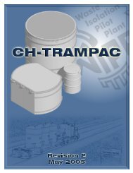
Locations of the WlPP Site and Tested Wells .............................................................................. 18 

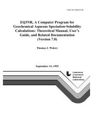
WIPP-Area Stratigraphic Column .................................................................................................. 19 

Well Configuration for H-1 Slug Tests .......................................................................................... 21 

Well Configuration for H-4c Slug Test .......................................................................................... 22 

Plan View of the Wells at the H-8 Hydropad ................................................................................ 22 

Well Configuration for H-8b Pumping Test .................................................................................. 23 

Well Configuration for H-12 Slug Tests ........................................................................................ 23 

As-Built Configuration for Well H-14 ............................................................................................. 24 


As-Built Configuration and +Packer Completion for Well H-16 ................................................. 26 



Well Configuration for WIPP-12 Castile and Salado Testing ...................................................... 28 

Well Configuration for WIPP-12 Culebra Slug Tests ................................................................... 28 

Well Configuration for WIPP-18 Slug Test ................................................................................... 29 




Well Configuration for WlPP-30 Slug Tests ................................................................................. 31

3-18 

3-19 

3-20 

3-21 

3-22 

3-23 

3-24 

3-25 

4-1 

51 

52 

Well Configuration for P-15 Slug Tests ........................................................................................ 32 

Well Configuration for P-17 Slug Tests ........................................................................................ 32 

Well Configuration for P-18 Slug Test .......................................................................................... 33 

Well Configuration for ERDA-9 Slug Tests ................................................................................... 34 

Well Configuration for Cabin Baby-1 Slug Tests ......................................................................... 34 

Well Configuration for DOE-1 Pumping Test ............................................................................... 35 

Well Configuration for Engle Pumping Test ................................................................................ 35 

Well Configuration for Carper Pumping Test ............................................................................... 36 

Components of a Drillstem Test and Slug Test ........................................................................... 38 

WIPP-l2/Brine Reservoir Plug Test Linear-Linear Sequence Plot . 42 

WIPP-l2/Upper Castile and Plug Test Linear-Linear Sequence Plot . 43 

53 

54 

55 

WIPP-12/lnfra-Cowden Test Linear-Linear Sequence Plot ......................................................... 45 

WIPP-12/lnfra-Cowden First Buildup Homer Plot ........................................................................ 45 

WlPP-I2/Salado Marker Bed 136 to Cowden Test Linear- 

Linear Sequence Plot ................................................................................................................ 46 

5-6 WIPP-l2/Salado Marker Bed 136 to Cowden First 

Buildup Homer Plot ................................................................................................................... 46 

57 WIPP-l2/Salado Marker Bed 103 to Cowden Test Linear- 


58 WIPP-1 2/Salado Marker Bed 103 to Cowden First Buildup 

Homer Plot ................................................................................................................................. 48 

59 WIPP-l2/Salado Casing to Cowden Test Linear- 


51 0 WlPP-l2/Salado Casing to Cowden First Buildup 

Homer Plot ................................................................................................................................. 49 

51 1 H-16AJnnamed Lower Member Siltstone Drillstem Test 

Linear-Linear Sequence Plot .................................................................................................... 51 

512 H-1 6Nnnarned Lower Member Siltstone First Buildup 

Log-Log Plot with INTERPRET Simulation .............................................................................. 51 

51 3 H-16Rlnnamed Lower Member Siltstone First 

Buildup Dimensionless Homer Plot with 

INTERPRET' Simulation ............................................................................................................. 55 

10

514 

5-15 

5-16 

5-17 

5-18 

5-19 

5-20 

5-21 

5-22 

523 

5-24 

5-25 

5-26 

5-27 

5-28 

529 

530 

5-31 

5-32 

5-33 

534 

H-I 6Nnnamed Lower Member Siltstone Second 

Buildup Log-Log Plot with INTERPRET Simulation ................................................................ 55 

H-1 6/Unnamed Lower Member Siltstone Second 

Buildup Dimensionless Horner Plot with 

INTERPRET Simulation ............................................................................................................. 57 

H-l/Culebra Slug-Test #1 Plot ...................................................................................................... 58 

H-1ICulebra Slug-Test #2 Plot ...................................................................................................... 58 



H&/Culebra Post-Acidization Slug-Test Plot ............................................................................. 62 

H-8bjCulebra Pumping Test Drawdown Log-Log 

Plot with INTERPRET Simulation .............................................................................................. 64 

H-ablCulebra Pumping Test Recovery Log-Log 


H-8 b/Cu le bra Pumping Test Linea r-Li n ear 

Sequence Plot with INTERPRET Simulation ........................................................................... 65 

H-l2/Culebra Slug-Test XI Plot ................................................................................................... 66 

H-l2/Culebra Slug-Test #2 Plot ................................................................................................... 67 

H-l4/Upper Culebra Drillstem Test Linear- 


H-I4/Upper Culebra First Buildup Log-Log 


H-l4/Upper Culebra First Buildup Dimensionless 

Horner Plot with INTERPRET Simulation ................................................................................. 69 

H-I 4/Upper Culebra Second Buildup Log-Log 


H-l4/Upper Culebra Second Flow Period Early- 

Time Slug-Test Plot ................................................................................................................... 71 

H-l4/Complete Culebra Drillstem and Slug 

Testing Linear-linear Sequence Plot ...................................................................................... 71 

H-l4/Culebra First Buildup Log-Log Plot with 


H-l4/Culebra Second Buildup Log-Log Plot 

with INTERPRET Simulation ..................................................................................................... 72 

H-l4/Culebra Slug-Test Plot ......................................................................................................... 73

5-35 H-l5/Culebra Drillstem and Slug Testing 

tinear-Linear Sequence Plot .................................................................................................... 74 

5-36 

5-37 



H-l5/Culebra First Buildup Dimensionless 

Homer Plot with INTERPRET Simulation ................................................................................. 76 

5-38 H-l5/Culebra Second Buildup Log-Log Plot 


5-39 H-1 5/Culebra Second Buildup Dimensionless 


5-40 

541 

542 

H-l5/Culebra Slug-Test Plot .......................................................................................................... 78 

H-lG/Culebra Drillstem and Slug Testing 

tinear-tinear Sequence Plot .................................................................................................... 78 

H-16ICulebra First Buildup Log-Log Plot with 


5-43 H-1 G/Culebra First Buildup Dimensionless 


5-44 H-lG/Culebra Second Buildup Log-Log Plot 


5-45 H-1 G/Culebra Second Buildup Dimensionless 


546 

5-47 

H-lG/Culebra Slug-Test Plot ......................................................................................................... 82 

H-l7/Culebra Drillstem and Slug Testing 


5-48 H-l7/Culebra First Buildup Log-Log Plot with 


549 H-l7/Culebra First Buildup Dimensionless 


5-50 H-17lCulebra Second Buildup Log-Log Plot 


5-51 H-lir/Culebra Second Buildup Dimensionless 


5-52 

553 

H-l7/Culebra Slug-Test Plot ......................................................................................................... 86 

H-l8/Culebra Drillstem and Slug Testing 

tinear-tinear Sequence Plot .................................................................................................... 87

5-54 

5-55 

5-56 

5-57 

5-58 

5-59 

5-60 

5-6 I 

5-62 

5-63 

5-64 

5-65 

5-66 

5-67 

5-68 

5-69 

5-70 

5-71 

5-72 

5-73 

5-74 

5-75 

5-76 

5-77 



H-181Culebra First Buildup Dimensionless 


H-l8/Culebra Second Buildup Log-Log Plot 

with INTERPRn Simulation ..................................................................................................... 89 

H-l8/Culebra Second Buildup Dimensionless 


H-l8/Culebra Slug-Test Plot ......................................................................................................... 90 

WIPP-l2/Culebra Slug-Test #1 Plot ............................................................................................. 91 

WIPP-lP/Culebra Slug-Test #2 Plot ............................................................................................. 91 

WIPP-lE)/Culebra Slug-Test Plot ................................................................................................... 92 

WIPP-lS/Culebra Slug-Test Plot ................................................................................................... 93 

WIPP-Pl/Culebra Slug-Test Plot ................................................................................................... 93 

WIPP-22/Culebra Slug-Test Plot ................................................................................................... 94 

WIPP-30/Culebra Slug-Test #I Plot ............................................................................................. 95 

WIPP90/Culebra Slug-Test #2 Plot ............................................................................................. 95 

P-l5/Culebra Slug-Test #1 Plot .................................................................................................... 97 

P-lEi/Culebra Slug-Test #2 Plot .................................................................................................... 97 

P-l7/Culebra Slug-Test #1 Plot .................................................................................................... 98 

P-lir/Culebra Slug-Test #2 Plot .................................................................................................... 98 

P-lIJ/Culebra Slug-Test Plot .......................................................................................................... 99 

ERDA-S/Culebra Slug-Test #1 Plot .............................................................................................. 101 

ERDA-S/Culebra Slug-Test #2 Plot .............................................................................................. 101 

Cabin Baby-1ICulebra Slug-Test #1 Plot ..................................................................................... 102 

Cabin Baby-l/Culebra Slug-Test #2 Plot ..................................................................................... 102 

DOE-l/Culebra Pumping Test Drawdown Log-Log 


DOE-1ICulebra Pumping Test Recovery Log-Log 

Plot with INTERPRET Simulation .............................................................................................. 104

5-78 

5-79 

5-80 

5-81 

5-82 

5-83 

5-84 

5-85 

5-86 

5-87 

5-88 

5-89 

5-90 

5-91 

5-92 

5-93 

5-94 

5-95 

DOE-1ICulebra Pumping Test Recovery 

Dimensionless Horner Plot with INTERPRET 

Simulation .................................................................................................................................. 105 

DOE-1 ICulebra Pumping Test Linear-Linear 

Sequence Plot with INTERPRET Simulation ........................................................................... 106 

Engle/Culebra Pumping Test Drawdown Log-Log 


Engle/Culebra Pumping Test Drawdown 


Simulation .................................................................................................................................. 107 

H-14flamarisk Claystone Shut-In Test Linear- 


H-1 6/Tamarisk Claystone Shut-In Test Linear- 


H-l4/Magenta Drillstem Test Linear-Linear 

Sequence Plot ........................................................................................................................... 11 1 

H-l4/Magenta First Buildup Log-Log Plot 

with INTERPRET Simulation ..................................................................................................... 1 12 

H-l4/Magenta Second Buildup Log-Log Plot 


H-l4/Magenta Second Buildup Dimensionless 


H-l4/Magenta Third Buildup Log-Log Plot 


H-l4/Magenta Third Buildup Dimensionless 

Horner Plot with INTERPRE Simulation ................................................................................. 114 

H-lG/Magenta Drillstem and Slug Testing 

Linear-Linear Sequence Plot .................................................................................................... 1 16 

H-1 G/Magenta First Buildup Log-Log Plot 


H-1 6lMagenta Second Buildup Log-Log Plot 


H-1 6/Magenta Drillstem Test Linear-Linear 

Plot with INTERPRET Simulation .............................................................................................. 11 7 

H-1 G/Magenta Early-Time Slug-Test Plot ..................................................................................... 1 18 

H-l4/Forty-Niner Claystone Drillstem and 

Slug Testing Linear-Linear Sequence Plot .............................................................................. 119

5-96 H-l4/Forty-Niner Claystone First Buildup 


5-97 H-l4/Forty-Niner Claystone First Buildup 


Simulation .................................................................................................................................. 121 

5-98 H-l4/Forty-Niner Claystone Second Buildup 

Log-Log Plot with INTERPRET Simulation ............................................................................. ,122 

5-99 H-14/Forty-Niner Claystone Early-Time 

5-1 00 

5-101 

5-102 

Slug-Test Plot ............................................................................................................................. 122 

H-14/Forty-Niner Anhydrite Drillstem Test 


H-lG/Forty-Niner Clay Pulse, Drillstem, and 

Slug Testing Linear-Linear Sequence Plot .............................................................................. 124 

H-lG/Forty-Niner Clay Pulse-Test Plot .......................................................................................... 125 

5-1 03 H-1 6IForty-Niner Clay First Buildup Log-Log 


5-104 H-lGIForty-Niner Clay First Buildup 


Simulation .................................................................................................................................. 126 

5-1 05 H-lG/Forty-Niner Clay Second Buildup Log-Log 


5-1 06 H-1 G/Forty-Niner Clay Early-Time Slug-Test 

Plot .............................................................................................................................................. 127 

5-1 07 H-lI/Lower Dewey Lake Drillstem and Pulse 

Testing Linear-Linear Sequence Plot ...................................................................................... 128 

5-1 08 Carper/Cenozoic Alluvium Pumping Test Drawdown 


5-1 09 Carper/Cenozoic Alluvium Pumping Test Drawdown 


Simulation .................................................................................................................................. 130 

6-1 

6-2 

Culebra Wells Tested by the WlPP Project .................................................................................. 132 

Distribution of Rustler Halite and Culebra 

Transmissivity Around the WlPP Site ....................................................................................... 133 

6-3 Vertical Hydraulic-Head Relations Among the 

Rustler Members at the WlPP Site .......................................................................................... 137 

A-1 Single-Porosity Type Curves for Wells with 

Wellbore Storage and Skin ....................................................................................................... 146

A-2 

A-3 

A4 

A-5 

A-6 

Single-Porosity Type Curves and Pressure- 

Derivative Type Curves for Wells with 

Wellbore Storage and Skin ....................................................................................................... 147 

Double-Porosity Type Curves for Wells with 

Wellbore Storage. Skin. and Restricted 

lnterporosity Flow ...................................................................................................................... 152 

Double-Porosity Type Curves for Wells with 

Wellbore Storage. Skin, and Restricted 

lnterporosity Flow ...................................................................................................................... 154 

Semilog Slug-Test Type Curves ................................................................................................... 158 

Eariy-Time Log-Log Slug-Test Type Curves ................................................................................ 158 

TABLES 

5-1 

5-2 

5-3 

Effective DST Flow Rates for Buildup Analyses .......................................................................... 52 

Summary of Non-Culebra Single-Well Test Results ................................................................... 54 

Summary of Culebra Single-Well Test Results ........................................................................... 60

INTERPRETATIONS OF SINGLE-WELL HYDRAULIC TESTS 

CONDUCTED AT AND NEAR THE WASTE ISOLATION 

PILOT PLANT (WIPP) SITE, 1983-1987 

1. INTRODUCTION 

This report presents the results of single-well 

hydraulic tests performed in 23 wells in the vicinity of 

the Waste Isolation Pilot Plant (WIPP) site in 

southeastern New Mexico (Figure 1-11 between 1983 

and 1987. The WlPP is a US. Department of Energy 

research and development facility designed to 

demonstrate safe disposal of transuranic radioactive 

wastes resulting from the nation’s defense programs. 

The WlPP facility will lie in bedded halite in the lower 

Salado Formation. The tests reported herein were 

conducted in the Salado Formation, in the underlying 

Castile Formation, and in the overlying Rustler 

Formation, Dewey Lake Red Beds, and Cenozoic 

alluvium. These tests were performed under the 

technical direction of Sandia National Laboratories, 

Albuquerque, New Mexico. 

Most of the tests discussed in this report were 

performed in the Culebra Dolomite Member of the 

Rustler Formation. The Culebra was tested at wells 

H-1, H-~c, H-8b, H-12, H-14, H-15, H-16, H-17, H-18, 

WIPP-12, WIPP-18, WIPP-19, WIPP-21, WIPP-22, 

WIPP-30, P-15, P-17. P-18, ERDA-9, Cabin Baby-1 , 

DOE-I, and Engle. The Forty-niner, Magenta, and 

Tamarisk Members of the Rustler were tested in H-14 

and H-16. The unnamed lower member of the 

Rustler Formation was tested in H-16. The Dewey 

Lake Red Beds were tested in well H-14. Alluvium of 

Cenozoic age was tested in the Carper well. The 

Castile and Salado Formations were tested in WIPP- 

12. With the exception of additional testing 

performed at DOE-2 that has been previously 

reported by Beauheim (1 986), this report discusses 

all single-well testing initiated by Sandia and its 

subcontractors at the WlPP site from 1983 through 

1987. 

17

'H-6 

o DOE-2 

OHIPP-13 

OAIPP 12 

OH-18 OWPP-18 

OH-14 

0 H-3 

*DOE-1 

1-5 

-WIPP-SITE 

BOUNDARY 

0p-18 

F-15 

0 n-11 

.H.AC 

*CABIN EABV 

OP-1' 

OW17 

0 H-12 

H-lo 0 

0 H-9 

ENGLE 0 

0 

- 

SCALE 

Figure 1-1. Locations of the WlPP Site and Tested Wells

2. SITE HYDROGEOLOGY 

The WlPP site is located in the northern part of the 

Delaware Basin in southeastern New Mexico. WIPPsite 

geologic investigations have concentrated on 

the upper seven formations typically found in that 

part of the Delaware Basin. These are, in ascending 

order, the Bell Canyon Formation, the Castile 

Formation, the Salado Formation, the Rustler 

Formation, the Dewey Lake Red Beds, the Dockum 

Group, and the Gatuna Formation (Figure 2-1). All of 

these formations are of Permian age, except for the 

Dockum Group, which is of Triassic age, and the 

Gatuna, which is a Quaternary deposit. Of these 

formations, the Bell Canyon and the Rustler contain 

the most-transmissive, regionally continuous 

saturated intervals. 

SYSTEM 

RECENT 

OUATER- 

NARY 

rRlASSlC 

z 

5 

5 

Y 

a 

- 

SERIES 

RECENT 

'LEISTO- 

CENE 

Figure 2-1. 

FORMATION 

iURFlClAL DEPOSITS 

IESCALERO CALICHE 

GATUNA 

UNDIVIDED 

DEWEY LAKE 

RED BEDS 

RUSTLER 

SALAD0 

CASTILE 

BELL CANYON 

CHERRY 

CANYON 

BRUSHY 

CANYON 

WIPP-Area Stratigraphic 

Column 

MEMBER 

Forfv-niner 

Magenta Dolomite 

Tamarisk 

Culebra Dolomite 

unnamed 

Vaca Trirte Sandstone 

Cowden Anhvdrile 

The Castile Formation at the WlPP site is composed 

of five informal members (in ascending order): 

Anhydrite I, Halite I, Anhydrite II, Halite II, and 

Anhydrite 111. Apart from isolated brine reservoirs 

sometimes found in fractured portions of the upper 

Castile anhydrites (Popielak et al., 1983), little is 

known about Castile hydrology because of the 

extremely low permeabilities of the unfractured 

anhydrite and halite units (Mercer, 1987). 

The Salado Formation is approximately 2000 ft thick 

at the WlPP site, and is composed largely of halite, 

with minor amounts of interspersed clay and 

polyhalite. The Salado also contains interbeds of 

anhydrite, polyhalite, clay, sylvite, and langbeinite. 

Jones et al. (1960) labeled several of the anhydrite 

and/or polyhalite interbeds that are traceable over 

most of the Delaware Basin "Marker Beds" and 

numbered them from 101 to 145, increasing 

downward. The WIPP facility horizon lies between 

Marker Beds 138 and 139. Because of the extremely 

low permeability of halite, few hydraulic tests have 

been attempted in the Salado, and little is known 

about Salado hydrology (Mercer, 1987). 

At the locations where the Rustler Formation was 

tested, its top lies from 231 (P-15) to 692 ft (H-15) 

below ground surface, and its bottom lies from 542 

(P-15) to 1088 ft (P-18) deep. At these locations, the 

Rustler consists of five mappable members (in 

ascending order): the unnamed lower member, the 

Culebra Dolomite Member, the Tamarisk Member, 

the Magenta Dolomite Member, and the Forty-niner 

Member. The unnamed lower member is composed 

of a layered sequence of clayey siltstone, anhydrite, 

and halite (absent on the western side of the WlPP 

site) ranging from 95 (WIPP-30) to 150 ft (P-18) thick. 

The Culebra is a light olive-gray, fine-grained, vuggy, 

silty dolomite, 21 (WIPP-18) to 29 ft (P-18) thick. The 

Tamarisk Member is composed of two anhydrite 

and/or gypsum units with a silty-claystone interbed 

which contains halite along the southern and central 

portions of the eastern boundary of the WlPP site. 

The Tamarisk has a total thickness of 84 (WIPP-19, 

ERDA-9, DOE-I) to 179 ft (P-18). The Magenta 

Dolomite Member consists of a silty, gypsiferous, 

laminated dolomite, 22 (H-8b) to 27 ft (P-15) thick. 

The Forty-niner Member consists of two 

anhydritelgypsum units separated by a silty 

claystone interbed which contains halite east of the 

19

WlPP site. The aggregate thickness of the Fortyniner 

varies between 55 (DOE-1) and 76 ft (P-18). 

All of the Rustler members are believed to be 

saturated. The Culebra dolomite is the most 

transmissive member, and is considered to be the 

most important potential groundwater-transport 

pathway for radionuclides which may escape from 

the WlPP facility to reach the accessible 

environment. Hence, the vast majority of hydrologic 

tests performed at the WlPP site have examined the 

hydraulic properties of the Culebra. The Magenta 

dolomite is generally considered to be the secondmost 

transmissive Rustler member, and has been 

tested at numerous locations by the US. Geological 

Survey (Mercer, 1983). Magenta hydraulic heads are 

generally higher than those of the Culebra. The 

other members of the Rustler are believed to have 

low permeabilities; few hydraulic tests have 

beenperformed on them and little is known about 

their hydraulic properties. 

The Dewey Lake Red Beds consist of siltstone with 

claystone and sandstone interbeds. Numerous 

bedding-plane breaks and fractures at various angles 

to the bedding are filled with secondary selenite. A 

well H-14, the Dewey Lake Red Beds are 320 ft thick, 

lying from 40 to 360 ft below ground surface. 

Continuous zones of saturation have not been 

observed within the Dewey Lake where it overlies the 

underground WlPP facility, although some minor, 

possibly perched, moist zones have been noted 

(Mercer, 1983). The Dewey Lake does provide small 

quantities of water to wells south and southwest of 

the WlPP site (Mercer, 1983). 

Cenozoic alluvium forms aquifers in much of the 

Delaware Basin, particularly in northern Texas. The 

alluvium consists of fluvial deposits, caliche, gypsite, 

conglomerates, aeolian sands, terrace deposits, and 

playa deposits (Richey et al., 1985). The alluvium is 

thickest in depressions caused by dissolution of the 

Salado. In southeastern Eddy County, the alluvium 

occurs past the erosional limit of the Dewey Lake 

Red Beds, and rests on an erosional/dissolution 

surface that moves progressively downsection from 

east to west from the Rustler to the Castile 

(Bachman, 1984). 

20

3. TEST WELLS 

Most of the wells discussed in this report were drilled 

from 1974 to 1987 for a variety of purposes. Many of 

them have been recompleted one or more times 

since the original drilling. Some of the wells are, or 

were, open holes through the strata tested, while 

others are cased and perforated to the tested 

intervals. The following sections contain brief 

histories of the wells, along with descriptions of their 

configurations at the times of testing. Unless 

otherwise indicated, all depths listed below are 

referenced to ground surface. 

3397.90 It 

7-inch. 26 Ib/ft ~ 

WELL CASING 

9.87Clnch 

REAMED BOREHOLE- 

3199. 

m n / I I I 

MAGENTA DOLOMITE 

sas n - m 

397.7 n- 

34w 18 n 

2 375-Inch TUBING 

TRANSDUCER 

3.1 H-1 

Well H-1 was drilled in May and June 1976 as the first 

hydrologic test hole for the Rustler Formation at the 

WlPP site. After drilling, selected coring, and openhole 

testing, the well was reamed to a diameter of 

9.875 inches to a total depth of 856 ft (Mercer and 

Orr, 1979). Seven-inch casing was installed and 

cemented from 848 ft to the surface, and a cement 

plug was left in the casing at a depth of 831 ft. Three 

sections of the casing were subsequently perforated 

using jet shots: the Rustler/Salado contact zone 

between 803 and 827 ft; the interval between 675 

and 703 ft, including the Culebra from 676 to 699 ft; 

and the interval between 562 and 590 ft, including 

the Magenta from 563 to 589 ft. Following testing in 

1977, a retrievable bridge plug was set in the casing 

at about 790 ft, and a production-injection packer 

(PIP) was set on 2.375-inch tubing at about 651 ft. 

This configuration allowed monitoring of the Culebra 

water level through the 2.375-inch tubing, and 

monitoring of the Magenta water level in the annulus 

between the well casing and the tubing. The PIP was 

replaced with a similar PIP in July 1987 set from 

645.0 to 649.4 ft on 2.375-inch tubing. The Culebra 

interval was developed by bailing on August 27, 

September 1, and September 15,1987 in preparation 

for slug testing (Stensrud et al., 1988). A smalldiameter 

minipacker was set in the tubing 

temporarily at about 600 ft for use in the slug testing. 

The configuration of H-1 at the time of the 1987 

testing is shown in Figure 3-1. 

wen 1//1 

CULEBRA DOLOMITE 

#@@e- 

TSOW- 

ALL DEPTHS BELOW GROUND SURFACE 

Figure 3-1. Well Configuration for H-1 

Slug Tests 

3.2 H-4~ 

NOT TO SCALE 

Well H-4c was originally drilled in April and May 1978 

to serve as a Rustler-Salad0 contact monitoring well. 

A 7.875-inch hole was drilled and reamed to a depth 

of 609.5 ft, and 5.5-inch casing was cemented from 

that depth to the surface. A 4.75-inch hole was then 

cored to a total depth of 661 ft, about 35 ft into the 

Salado Formation (Mercer et al., 1981). In February 

1981, a retrievable bridge plug was set in the casing 

at a depth of about 530 ft. The depth interval from 

494 to 520 ft was then shot-perforated to provide 

access to the Culebra. Mercer et al. (1981) report the 

Culebra at H-4c as lying between 490 and 516 ft 

21

deep. The gamma-ray log used to guide the 

perforation shows the Culebra from 489 to 515 ft 

deep, which indicates that the upper 4 to 5 ft of the 

Culebra are apparently not perforated at H-4c. For 

slug testing, a PIP was temporarily set in the casing 

from 479.2 to 483.6 ft deep on 2.375-inch tubing. 

Figure 3-2 shows the configuration of H-4c during the 

1986 slug test. 

depth of 624 ft. The Culebra at H-8 lies from 588 to 

614 ft below land surface (Wells and Drellack, 1982). 

The open interval in H-8b includes, therefore, the 

lower 13 ft of the Tamarisk Member, which consists 

of anhydrite and gypsum, the entire Culebra 

dolomite, and the upper 10 ft of the unnamed lower 

member of the Rustler, which consists of mudstone 

and gypsum. Only the Culebra portion of this interval 

is believed to have significant permeability. For 

testing in 1985, a pump was installed in the well 

below a packer set from 557.7 to 561.9 ft on 1 S-inch 

galvanized pipe. The configuration of the well at the 

time of the December 1985 pumping test is shown in 

Figure 3-4. 

2.375-inch TUBING 

H-8a (MAGENTA) 

5.5-inch, 15.5 Ib/ff 

WELL CASING 

7.875-inch 

REAMED BOREHOLE 

ANNULUS TRANSDUCER 

DRUCK PDCR lOlD 

TEST-INTERVAL TRANSDUCER 

DRUCK PDCR 10tD 

BASK1 PACKER 

H-8b (CULEBRA) 

BRIDGE PLUG 


NOT TO SCALE 

Figure 3-2. Well Configuration for H-1 Slug Tests 

3.3 H-8b 

Figure 3-3. 

Pian View of the Wells at the 

H-8 Hydropad 

Well H-8b was drilled in August 1979 by the USGS as 

one of 3 wells in the H-8 borehole complex 

(Figure 3-3). The hole was drilled and reamed to a 

diameter of 9.75 inches down to 575 ft, and 7-inch 

casing was set and cemented from 574 ft to the 

surface. A 6.125-inch hole was then cored to a total 

3.4 H-12 

Well H-12 was drilled in October 1983 to provide 

hydrologic and stratigraphic data southeast of the 

WlPP site. The hole was cored and reamed to a 

diameter of 7.875 inches to a depth of 820 ft, and 

22

~ 

2 

7-inch CASING 

9 75-inch REAMED BOREHOLE- , 

6 125-inch OPEN COREHOLE- 

TO 624H- 

ALL DEPTHSBELOW GROUND SURFACE 

-inch GALVANIZED PIPE 

ANNULUSTRANSDUCER 




BASK1 PACKER 

RED JACKET 32 BC PUMP 

PUMP INTAKE 

NOT TO SCALE 

37 I1 

' 70 I1 

620 n 

z 

z 

e 

K 

3 

3425 98 I1 

* 

HOLOCENE DEPOSITS 

678 11 

70311 

823 n 

850n 

DOCKUM GROUP 

DEWEY 

LAKE 

RED 

BEDS 

3427 19 1t 

9 875-inch. 40 Ibltf 

CONDUCTOR CASING 

2 375-lnch TUBING 

FORTY- 

NINER -7 875-inch 

MEMBER 


MAGENTA 

DOLOMITE 

MEMBER 

TAMARISK 

MEMBER 

CULEBRA 

DOLOMITE 

MEMBER 

4.75-Inch OPEN HOLE 

PLUGGED BACK 

LOWER DEPTH 890 11 

MEMBER 

CEMENT PLUG 

980 n 

SALAD0 FORMATION -TOTAL DEPTH 1W1 I( 

4LL DEPTHS BELOW GROUND SURFACE 

NOT TO SCALE 

Figure 3-4. 

Well Configuration for H-8b 

Pumping Test 

Figure 3-5. Well Configuration for H-12 

Slug Tests 

5.5-inch casing was cemented from that depth to the 

surface (HydroGeoChem, 1985). The hole was then 

deepened to 1001 ft, 21 ft into the Salad0 Formation, 

by coring and reaming to a diameter of 4.75 inches. 

The bottom of the hole was plugged back with 

cement to a depth of 890 ft. As a result, the well is 

open to the lower 3 ft of the Tamarisk from 820 to 

823 ft, the Culebra from 823 to 850 ft, and the 

unnamed lower member of the Rustler from 850 to 

890 ft. The well was developed by bailing on July 10, 

13, 15, and 17, 1987 in preparation for slug testing 

(Stensrud et al., 1988). A PIP on 2.375-inch tubing 

was set in the well casing from 810.3 to 814.7 ft from 

August to September 1987 to aid in testing. In 

addition, a minipacker was set in the tubing at about 

484 ft. The configuration of H-12 at the time of 


3.5 H-14 

H-14 was drilled in October 1986 to provide a 

Culebra monitoring well in the southwest quadrant of 

the WlPP site where no other Culebra wells existed 

(see Figure 1-1). A 7.875-inch hole was drilled and 

reamed to a depth of 533 ft, stopping about 12 ft 

above the Culebra. After the Tamarisk, Magenta, 

Forty-niner, and Dewey Lake Red Beds were tested, 

5.5-inch casing was set and cemented from 532 ft to 

the surface. A 4.5-inch hole was then cored to 574 ft. 

Following Culebra tests, the hole was reamed to 

4.75 inches, and deepened to the final depth of 

589 ft. Stratigraphic depths of the formation 

encountered and the final as-built configuration of H- 

14 are shown in Figure 3-6. 

23

3347.11 ft 

\ 

- 

-12.25-inch HOLE 

-8.625-inch, 28 Ibllt 

\ ;9YDUCTOR CASING 

1 

12.25-inch HOLE 

68.625-Inch. 28 lblfl 

;9;DUfXOR CASING 

- 

-7.875-inch 


-7.875-Inch 


-5.5-inch. 

15.5 Ib/ft WELL CASING 

-5.5-inch. 

15.5 lblfi WELL CASING 

- 532 ff 

IL 

L 

TAMARISK 

-853ll 

-4.75-inch 

OPEN HOLE 

- 4.75-inch OPEN HOLE 

MEMBER 


-TOTAL DEPTH 589 11 

NOT TO SCALE 

MEMBER 

ALLOEPTHSBELOW GROUND SURFACE 

- TOTAL DEPTH 900 I! 

NOT TO SCALE 

Figure 3-6. As-Built Configuration for Well H-14 

3.6 H-15 

H-15 was drilled in November 1986 to provide a 

Culebra monitoring well in the east-central portion of 

the WlPP site where no other Culebra wells existed 

(see Figure 1-1). A 7.875-inch hole was drilled to a 

depth of 854 ft, about 7 ft above the top of the 

Culebra, and 5.5-inch casing was set and cemented 

from 853 ft to the surface. The hole was then cored 

and reamed through the Culebra to about 891 ft to a 

diameter of 4.75 inches. Following tests of the 

Culebra, the hole was deepened at a diameter of 

4.75 inches to its final depth of 900 ft. Stratigraphic 

depths of the formations encountered and the final 

as-built configuration of the well are shown in 

Figure 3-7. 


3.7 H-16 

H-16 was drilled in July and August 1987 to provide a 

location to monitor the hydraulic responses of the 

members of the Rustler during construction of the 

WIPP Air-Intake Shaft. A hole was rotary-drilled and 

reamed to a diameter of 9.625 inches to a depth of 

470 ft, and 7-inch casing was installed and cemented 

in place from the surface to a depth of 469 ft. The 

hole was deepened in five steps to its final total 

depth of 850.9 ft. Each member of the Rustler was 

successively cored and reamed to a 4.75-inch 

diameter. Drillstern, slug, andfor pulse tests were 

performed on each member before the next member 

was cored. After all testing was finished, the hole 

24

was reamed to a final diameter of 6.125 inches. The 

well was completed by installing a 5-packer system 

that isolates each of the Rustler members and allows 

monitoring of fluid pressure in each member. 

Stratigraphic depths of the formations encountered 

and the 5-packer completion of the well are shown in 

Figure 3-8. 

3.0 H-17 

Well H-17 was drilled from September to November 

1987 to investigate an area south of the WlPP site 

that was believed, on the basis of computer 

modeling (Haug et al., 1987) and surface 

geophysical surveys (Bartel, in preparation), to have 

high transmissivity in the Culebra. A 7.875-inch hole 

was drilled to a depth of about 510 ft, just below the 

top of the Rustler Formation. The hole was then 

cored to a depth of 693 ft, about 13 ft above the top 

of the Culebra. After reaming to 9.625 inches, 7-inch 


surface. The hole was then cored and reamed 

through the Culebra to about 735 ft to a diameter of 

4.75 inches. Following testing of the Culebra, the 

hole was cored to 870.3 ft for stratigraphic 

information, reamed to 6.1 25 inches for geophysical 

logging, and then plugged back to 773 ft with 

cement. Stratigraphic depths of the formations 

encountered and the final as-built configuration of 

the well are shown in Figure 3-9. 

3.9 H-18 

Well H-18 was drilled in October and November 1987 

to investigate an area in the northwest portion of the 

WlPP site where large changes in Culebra 

transmissivity and water quality occur. A 9.625-inch 

hole was cored and reamed to a depth of 674 ft, 

about 15 ft above the top of the Culebra, and 7-inch 


surface. The hole was then cored and reamed 

through the Culebra to about 714 ft to a diameter of 

4.75 inches. Following testing of the Culebra, the 

hole was cored to 830.5 ft for stratigraphic 

information, reamed to 6.1 25 inches for geophysical 

logging, and then plugged back to 766 ft with 

cement. Stratigraphic depths of the formations 

encountered and the final as-built configuration of 

the well are shown in Figure 3-10. 

3.10 WIPP-12 

Drilling began at WIPP-12 in November 1978. The 

hole was drilled and reamed to a diameter of 

12.25 inches to a depth of about 1003 ft, and 

9.625-inch casing was set and cemented from 1002 ft 

to the surface. The hole was then cored and reamed 

to a diameter of 7.875 inches to a total depth of about 

2774 ft, approximately 48 ft into the Castile Formation 

(Sandia and D’Appolonia, 1982). As the borehole 

was being deepened in 1981, a pressurized brine 

reservoir was encountered at a depth of about 301 7 ft 

in the lower portion of the Anhydrite 111 unit of the 

Castile (Popielak et al., 1983). The hole was 

deepened at a diameter of 7.875 inches to about 

3107 ft, from which point the diameter was reduced 

to 6 inches for the balance of the hole down to the 

total depth of 3927.5 ft in the upper part of the 

Anhydrite I unit of the Castile (Black, 1982). In June 

1983, the upper part of the wellbore was isolated 

from the brine reservoir by setting a bridge plug in 

the hole from 3000 to 3005 ft deep, putting 27 ft of 

sand on top of the bridge plug, and putting a 1894 

cement plug on top of the sand (D’Appolonia, 1983). 

Key stratigraphic horizons and the well configuration 

at the time of the August-September 1985 testing are 

shown in Figure 3-1 1. 

On October 12, 1985, a retrievable bridge plug was 

set in the WIPP-12 casing between the depths of 

984.0 and 989.4 ft. Two days later, gamma-ray 

logging was performed which indicated that the 

Culebra interval extended from 815 to 840 ft below 

ground surface, and that interval was then shotperforated. 

All stratigraphic contacts shown on this 

log are approximately 5 ft deeper than those reported 

by Sandia and D’Appolonia (1982). This discrepancy 

may be due to the 1978 and 1985 logging surveys 

having used different datums to “zero” their depth 

counters. Inasmuch as the 1985 gamma-ray log and 

the perforation were run off the same depth counter 

and used the same datum, the correct Culebra 

interval should have been perforated. 

25

~ 

3409.6 n 

__ - - 

HOLOCENE DEPOSITS 

.-.. 

37 11 GATUNA FORMATION 

DOCKUMGROUP 

3406 8 1 

~- L 

\ 

3408 0 11 


10.75-inch. 40 lbllt 


-9.625-inch 


DEWEY 

LAKE 

RED 

BEDS 

PACKER-INFLATION LINES 

7-inch. 23 Ib/ft 

WELL CASING 


TRANSDUCER CABLES 

531.9 II 

a 

u 

m 

5 

I 562 6 11 

a 

Y 

z 

f 

I- 

a 

z 

590 2 If 

615 6 11 

573 8 11 

ANHYDRITE/ 

GYPSUM 

CLAY (STONE) 

ANHYDRITE) 

GYPSUM 

MAGENTA DOLOMITE 

MEMBER 

__ 469 It 

TRANSDUCER U5. SIN 2472 

TRANSDUCER 04. SIN 2475 

3 

m 

s 

Y 

2 

U 

a 

3 

ANHY DRlTE' 

GYPSUM 

671 5 It 

CLAYSTONE 

690, 

ssssn-, GYPSUM 

CLAYSTONEISILTSTONEISANDSTC 

702 5 I l l 

724 4 If 

U 

w 

m 

; 

re 

f 

3 

n 

lu 

2 

z 

2 

3 

733 3 Ii 

742 4 W 

777 7 n 

CULEBRA DOLOMITE 

MEMBER 

CLAY STONE 

GYPSUM 

HALlTlC CLAYSTONE! 

HALITE 

GYPSUM 

SILTSTONE/ 

CLAYSTONE 

-747 5 It 

_t__ 

TRANSDUCER #3. SIN 2474 

TRANSDUCER U2. SIN 2105 

TRANSDUCER Ul. SIN 2174 

800-psi SHEAR-PIN PLUG 

6.125-inch OPEN HOLE 

GYPSUMA/HALITE/POLYHAI 

841.5 n 

SALAD0 FORMATION 

1- TOTAL DEPTH 850 9 I! 


NOT TO SCALE 

Figure 3-8. As-Built Configuration and 5-Packer Completion for Well H-16

33M.01 tf 

2, HOLOCENE DEPOSITS 

5.31 ft 


.-4 

3413.36 It 

14 21 If 


10.75-inch. 40 ib/H 



9.625-inch 


7-inch. 23 Ib/ll 

WELL CASING 

?-inch, 23 Iblft 

WELL CASING 

DOLOMITE 

TAMARISK 

MEMBER 

I 

I 

t -6,125-inch 

-PLUGGED BACK 

DEPTH 773 ft 

-CEMENT 

PLUG 

-TOTAL 

DEPTH 870 3 II 

OPEN HOLE 

Y -I 

t-u) 

3 

C 

608.6n 

MEMBER 

- 6.125-Inch OPEN HOLE 


NOT TO SCALE 

-TOTAL 

CEMENT PLUG 

DEPTH 830.5 fl 


NOT TO SCALE 


'IPP-12 was pumped briefly on May 1, 198 to 

develop the perforations and to provide information 

useful in designing a testing program (Saulnier et al., 

1987). The well yielded very little water, indicating 

low transmissivity and/or a poor hydraulic connection 

between the well and the formation. In an effort to 

improve the effectiveness of the casing perforations 

in connecting the well with the formation, the well 

was acidized on May 21 , 1986. About 50 gallons of a 

20% hydrochloric-acid solution were injected into the 

perforations under a surface pressure of 300 to 

500 psig over 95 minutes. Because the acid solution 

was not readily injected, 500 gallons of the acid 

solution were placed at and above the Culebra 

perforations, and further well-development work was 

deferred. 

The spent acid solution and other wellbore fluids 

were bailed from WIPP-12 on August 27 and 28, 

1987. After the fluid level recovered, a pump was set 

Figure 3-10. As-Built Configuration for Well H-I 8 

in the well and all fluids were pumped from the well 

on 3 occasions in October and November 1987. The 

pump was then removed, and the well was bailed 

again on December 8, 1987. The fluid removed on 

this occasion was used to inflate a PIP set in the well 

casing on 2.375-inch tubing from 794.4 to 796.0 ft on 

December 16, 1987. A small-diameter minipacker 

was set in the tubing from 601 .O to 602.8 ft. The PIP. 

tubing, and minipacker were removed from the well 

at the conclusion of testing. The configuration of 

WIPP-12 during the 1987 Culebra slug tests is shown 

in Figure 3-1 2. 

3.11 WIPP-18 

WIPP-18, WIPP-19, WIPP-21, and WIPP-22 were 

originally drilled in 1978 in the north-central portion 

of the WlPP site to investigate the structure of nearsurface 

formations after preliminary interpretations of 

seismic-survey data indicated the potential existence 

27

Ylf M (t 

-1wt 

5 n 

nch REAMED BOREHOLE 

nch. 32.3 Iblfl WELL CASING 

lbinch HOLE 

12.25-Inch 

REAMED BOREHOLE - 

2.375-inch 

TUBING 

::E:: MARKER BED 103 . 

z 

2 UNIONANHc 

< 

-4n 

207OIn MARKERBED’36 - 

Y 

0 

P 

< 

-I 

< 

Nu’n 

-,n 

COWDEN ANHYDRITE 

MEMBER 

7.87Cinch REAMED BOREHOLE 

O.(IZHnch, 323 IWft 

WELL CASING 

BASK1 1.5-inch PACKER 

ANNULUSTRANSDUCER 

DRUCK PDCR YOID 

RVAL TRANSDUCER 

I-< 

t? 

P 

CEMENT PLUG 

ANHYDRITE Ih 

0 BRIDGE PLUG 

ALL DEPTHS BELOW QROUWD WRFACE 

NOT TO SCALE 

BRIDGE PLUG 


NOT TO SCALE 

Figure 3-1 1. 

Well Configuration for WIPP-12 

Castile and Salado Testing 

of a fault in that vicinity (Sandia and USGS, 1980a). 

WIPP-18 was drilled to a total depth of 1060 ft, 132 ft 

into the Salado Formation, and no evidence of a fault 

was found. WIPP-18 was abandoned in an open-hole 

condition filled with brine mud until October 1985, 

when the hole was recompleted to serve as a 

Culebra observation well. To this end, the hole was 

reamed to a diameter of 7.875 inches, and 5.5-inch 

casing was installed and cemented from the surface 

to a depth of 1050 ft. The Culebra interval was then 

shot-perforated from 784 to 806 ft deep, based on 

gamma-ray logging performed to locate the Culebra. 

Sandia and USGS (1980a) report the Culebra at 

WIPP-18 as being from 787 to 808 ft deep. The 

discrepancy in depths was probably caused by the 

1978 and 1985 logging surveys using different 

datums to zero the tools. From May 10 to 14, 1986, 

WIPP-18 was developed by pumping and surging 

(Saulnier et al., 1987). For slug testing, a PIP was 

temporarily set in the well casing on 2.375-inch 

Figure 3-1 2. 


Culebra Slug Tests 

tubing from 769.7 to 774.0 ft. The configuration of 

the well at the time of testing is shown in Figure 3-13. 

3.12 WIPP-19 

WIPP-19 was drilled as part of the same program as 

WIPP-18 in 1978 (Sandia and USGS, 1980b). The 

hole was continuously cored to a total depth of 

1038.2 ft, 143.2 ft into the Salado Formation. 

WIPP-19 was then abandoned in an open-hole 

condition filled with brine mud until October 1985, 

when the hole was recompleted to serve as a 

Culebra observation well. The borehole was reamed 

to a diameter of 7.875 inches, and 5.5-inch casing 

was installed and cemented from the surface to a 

depth of 1036.6 ft. The Culebra interval was then 

shot-perforated from 754 to 780 ft deep, based on 

gamma-ray logging performed to locate the Culebra. 

Sandia and USGS (1980b), by comparison, report the 

Culebra as being 756 to 779 ft deep. From May 28 to 

28

3435.14 ff 1 



5.5-inch, 15.5 Ibffi 

WELL CASING 


DRUCK PDCR 10fD 

5.5-inch, 15.5 Ib/tI -.? 

WELLCASING 1 

ANNULUS TRANSDI UCER 



DRUCK PDCR 10ID 

7 n75 .inch 


LTEST-INTERVAL TRANSDUCER 


BASK1 PACKER 

m.uz n 

7.875-inch 


CASING PERFORATIONS 

784-806 n 

CULEBRA DOLOMITE 4 

1 CASING PERFORATIONS 

7 ~ - 7 ~ ) n 

1036.6 n--! 


%-CEMENT 

NOT TO SCALE 


NOT TO SCALE 

Figure 3-13. Well Configuration for WIPP-18 Slug Test 

29, 1986, the well was developed by pumping and 

surging (Saulnier et al., 1987). For slug testing, a PIP 

was temporarily set in the well casing from 737.5 to 

741.8 ft on 2.375-inch tubing. The configuration of 

the well at the time of testing is shown in Figure 3-14. 

3.13 WIPP-21 


WIPP-18 and WIPP-19 in 1978 (Sandia and USGS, 

1980~). The hole was drilled to a total depth of 

1046 ft, 178 ft into the Salado Formation. WIPP-21 

was then abandoned in an open-hole condition filled 

with brine mud until October 1985, when the hole 

was recompleted to serve as a Culebra observation 

well. The borehole was reamed to a diameter of 

7.875 inches, and 5.5-inch casing was installed and 


cemented from the surface to a depth of 1013.7 ft. 

The Culebra interval was then shot-perforated from 

727 to 751 ft deep, based on gamma-ray logging 

performed to locate the Culebra. Sandia and USGS 

(1980~) report the Culebra lies 2 ft lower, from 729 to 

753 ft deep, probably because of difference in the 

datums from which depths were measured. From 

June 28 to July 1, 1986, the well was developed by 

pumping and surging (Saulnier et al., 1987). For slug 

testing, a PIP was temporarily set in the well casing 

from 705.9 to 711.8 ft on 2.375-inch tubing. The 

configuration of the well at the time of testing is 

shown in Figure 3-15. 

29

3418.96 n 

7.875-inch 

REAMED BOREHOLE - 

TRAILER 



DRUCK PDCR IOlD 


DRUCK PDCR 101D 

BASK1 PACKER 

The depth discrepancy may be due to one of the two 

surveys having incorrectly "zeroed" a depth counter. 

Inasmuch as the 1985 survey and the subsequent 

perforation were run using the same depth counter 

and the same datum, the correct interval was 

probably perforated, whatever its true absolute 

depth. From June 11 to 17, 1986, WIPP-22 was 

developed by pumping and surging (Saulnier et al., 

1987). For slug testing, a PIP was temporarily set in 

the well casing from 738.1 to 742.5 ft on 2.375-inch 

tubing. The configuration of the well at the time of 


2.375-Inch TUBING 

5.5-inch. 15.5 Ib/n 

WELL CASING 

NNULUS TRANSDUCER 

RUCK PDCR lOlD 




NOT TO SCALE 

7.875-inch 


BASK1 PACKER 

Figure 3-1 5. Well Configuration for WIPP-21 Slug Test 

3.14 WIPP-22 


WIPP-18, WIPP-19, and WIPP-21 in 1978 (Sandia and 

USGS, 1980d). The hole was drilled to a total depth 

of 1448 ft, 565 ft into the Salado Formation. WIPP-22 

was then abandoned in an open-hole condition filled 

with brine mud until October 1985, when the hole 

was recompleted to serve as a Culebra observation 

well. The borehole was reamed to a diameter of 

7.875 inches, and 5.5-inch casing was installed and 

cemented from the surface to a depth of 949.8 ft. 

The Culebra interval was then shot-perforated from 

748 to 770 ft deep, based on gamma-ray logging 

performed to locate the Culebra. Sandia and USGS 

(1980d) report the Culebra 6 ft higher, from 742 to 

764 ft deep. The source of the 6-ft discrepancy 

between the 1978 and 1985 surveys is unknown. 


NOT TO SCALE 


3.15 WIPP-30 

Well WIPPBO was drilled in September 1978 as one 

of six wells drilled to evaluate dissolution of nearsurface 

rocks in and adjacent to Nash Draw (Sandia 

and USGS, 1980). WIPP-30 was cored and reamed to 

30

a diameter of 8.75 inches to a depth of 246 ft, and 

then deepened to 913 ft by coring and reaming to a 

diameter of 7.875 inches. Casing (5.5-inch) was 

installed and cemented from 912 ft to the surface. In 

March, July, and September 1980, three sections of 

the casing were perforated: the Rustler/Salado 

contact zone from 731 to 753 ft; the interval from 631 

to 654 ft which includes the Culebra from 631 to 

653 ft; and the interval from 510 to 540 ft which 

includes the Magenta from 513 to 537 ft (Seward, 

1982). Retrievable bridge plugs were set at depths 

of 688.5 and 590.7 ft in September 1980. In August 

1983, the upper bridge plug was replaced with a PIP 

set on 2.375-inch tubing at a depth of 570 ft to allow 

monitoring of the Culebra water level through the 

tubing, and the Magenta water level through the 

annulus between the casing and tubing. 

5.5-inch. 15.5 Ib/ff 


TEST-INTERVAL TRANSDUCE 


BASK1 7.5-inch PACKER 

3429 04 If 

3420 4I I T 

2 375-Inch TUBING 

ULUS TRANSDUCER 

In October 1987, the PIP was removed and the 

casing was reperforated between the depths of 629 

and 655 ft to improve the hydraulic connection 

between the Culebra and the well. In November 

1987, the well was bailed once and pumped 4 times 

(with both the Culebra and Magenta open to the well) 

to develop the perforations. On December 8, 1987, 

the well was pumped a final time to provide water for 

use in the subsequent slug tests, and a PIP was set 

from 613.1 to 617.5 ft in the well on 2.375-inch 

tubing. A minipacker was installed in the tubing from 

599.4 to 601.1 ft, and was removed after testing was 

completed. The configuration of WIPP-30 at the time 

of testing is shown in Figure 3-1 7. 

3.16 P-15 

Well P-15 was drilled in October 1976 as part of a 

21 -well evaluation program to investigate the potash 

resources in the Salado Formation at the proposed 

location of the WlPP site (Jones, 1978). P-15 was 

drilled and reamed to a diameter of 7.875 inches to a 

depth of 637 ft, and 4.5-inch casing was installed and 

cemented from 635 ft to the surface. The hole was 

deepened by coring at a 4-inch diameter to 1465 ft, 

and the bottom of the hole was plugged back to 

620 ft with cement (Mercer and Orr, 1979). In 

January and April 1977, two sections of the casing 

were perforated: the Rustler/Salado contact zone 

from 532 to 556 ft deep: and the intewal from 410 to 

438 ft which includes the Culebra from 413 to 435 ft. 


Figure 3-1 7. 

NOT TO SCALE 


Slug Tests 

A PIP was set in the casing at a depth of 512 ft on 

2.375-inch tubing to allow monitoring of 

Rustler/Salado and Culebra water levels. The PIP 

was determined to be leaking in May 1985, and was 

replaced on June 6, 1985 with a retrievable bridge 

plug set from 441 to 447 ft deep. 

P-15 was developed by bailing on March 27, April 7, 

16, and 21, 1987 in preparation for slug testing 

(Stensrud et al., 1988). A PIP on 2.375-inch tubing 

was set in the well casing temporarily from 389.6 to 

393.9 ft in May 1987 to aid in the testing. The 

configuration of P-15 at the time of testing is shown 

in Figure 3-18. 

3.17 P-17 

P-17 was drilled in October 1976 as part of the 

potash-resource evaluation program at the proposed 

location for the WlPP site (Jones, 1978). The hole 

was first rotary drilled at a diameter of 7.875-inches to 

a depth of 755 ft, approximately 40 ft into the Salado 

31


4.5-inch. 9.5 IblH 

WELL CASING 

ANNULUS TRANSDU 


BASK1 PACKER 



/ 

- 347.73 n 

-BASK1 1.5-inch PACKER 

- m.37 n 

I 

i- WS.(IZ n 

L- 393.91 it 

4.5-inch. 9.5 lbln 

WELL CASING 

7.875-inch 


2.37Cinch TUBING 


DRUCK PDCR 10ID 


DRUCK PDCR IOID 

7.875-inch 


BASK1 PACKER 

ASING PERFORATIONS 


CULL 

BRIDGE PLUG 


J 

BRIDGEPLUG 

NOT TO SCALE 


NOT TO SCALE 

Figure 3-19. Well Configuration for P-17 Slug Tests 

Figure 3-18. Well Configuration for P-15 Slug Tests 

Formation. Casing (4.5-inch diameter) was then set 

and cemented from 741 ft to the surface, and the 

hole was deepened at a 4-inch diameter to a total 

depth of 1660 ft. After coring was completed, the 

hole was plugged back to a depth of 731 ft with 

cement. In January and April 1977, two sections of 

the casing were perforated: the Rustler/Salado 

contact zone between 702 and 726 ft; and the 

interval from 558 to 586 ft, which includes the entire 

Culebra from 558 to 583 ft (Mercer and Orr, 1979). A 

PIP was set in the casing at 683 ft on 2.375-inch 

tubing to allow monitoring of Rustler/Salado and 

Culebra water levels. In March 1983, the PIP was 

replaced with a retrievable bridge plug set from 674 

to 679 ft. For testing in 1986, a PIP was temporarily 

set in the casing from 532.3 to 536.6 ft deep on 

2.375-inch tubing. The configuration of the well at 

the time of testing is shown in Figure 3-19. 

3.18 P-18 

Well P-18 was drilled in October and November 1976 

as part of the potash-resource evaluation program at 

the proposed WlPP site (Jones, 1978). The hole was 

drilled and reamed to a depth of 1139 ft at a diameter 

of 7.875 inches, and 4.5-inch casing was cemented 

from 1138 ft to the surface. The hole was then drilled 

and cored at a 4-inch diameter to a depth of 1998 ft, 

and plugged back to 1125 ft with cement. In January 

and April 1977, two sections of the casing were 

perforated: the RustlerlSalado contact zone between 

1076 and 1100 ft; and the interval from 912 to 940 ft, 

which includes most of the Culebra which lies 

between 909 and 938 ft (Mercer and Orr, 1979). In 

May 1977, a PIP was set on 2.375-inch tubing at a 

depth of 1061 ft to allow monitoring of Rustler/Salado 

and Culebra water levels. In early 1983, the PIP was 

removed and a bridge plug was set from 997 to 

32

1002 ft deep to allow testing of the Culebra. Testing 

consisted of a pressure-pulse test and a slug test, 

both of which indicated very low transmissivity, but 

were otherwise inconclusive. 

On June 12, 1987, the P-18 casing was reperforated 

from 909 to 938 ft to improve the hydraulic 

connection between the Culebra and the well. On 

June 16, 1987, a PIP was set in the well from 895.9 to 

899.2 ft deep on 2.375-inch tubing, and all fluid was 

bailed from the tubing. The tubing was bailed again 

on August 26, 1987, after the fluid level in the tubing 

had recovered. A minipacker was then installed in 

the tubing from 780.4 to 782.2 ft for use in 

subsequent testing. The configuration of the well at 

the time of testing is shown in Figure 3-20. 

34T7.M fl 

-1 

4.5-Inch, 9.5 Ib/ft- 

3478.42 fl 

WELL CASING 


DRUCK PDCR 10/D 

BASK1 1.5-inch PACKER- 

7.875-inch 

REAMED BOREHOLE- 

PRODUCTION-INJECTION- 

PACKER 

\ 

CULEBRA -"- DOLOMITE 

931"-1 

997fl- 


I 

I 

1 

I 

I 

I 

2.37Clnch TUBING 

,-- t 770.22 n 

780.39 fl 

-' 782.24fl 

\ 

r 

1 895.9011 

-, 899.2Ofl 


J 

BRIDGEPLUG 

NOT TO SCALE 

Figure 3-20. Well Configuration for P-18 Slug Test 

3.19 ERDA-9 

ERDA-9 was the first exploratory borehole for the 

proposed WIPP. It was drilled between April and 

June 1976 to provide stratigraphic and structural 

information on the Permian evaporites, as well as to 

provide core samples for further testing. When the 

bottom of the 15-inch hole was 1078 ft deep, 

10.75-inch casing was installed and cemented from 

the surface to a depth of 1033 ft, approximately 185 ft 

into the Salado Formation. After the hole was drilled 

to its finai total depth of about 2877 ft at a diameter of 

9.875 inches, it was completed by installing 7-inch 

casing from the surface to a depth of 2871 ft, and 

cementing only the lower 343 ft of that casing in 

place (Sandia and USGS, 1983). The hole was then 

left filled with a diesel-fuel-based drilling mud. 

ERDA-9 remained in this configuration until October 

1986, when it was recompleted as a Culebra 

observation well. During the recompletion, the upper 

980 ft of the 7-inch casing were cut off from the lower 

section and removed from the hole. A retrievable 

bridge plug was then set in the 10.75-inch casing 

from 758.9 to 760.6 ft deep, and the Culebra interval 

between 705.5 and 728.5 ft deep, as determined 

from a gamma-ray log, was shot-perforated using 4 

shotdft. Sandia and USGS (1983) reported the 

Culebra 1.5 ft higher, probably indicating that the two 

geophysical surveys did not use the same datum. 

From October 27 to November 14,1986, ERDA-9 was 

developed by pumping and surging. Additional 

recompletion and development information is 

contained in Stensrud et al. (1987). For slug testing, 

a PIP was temporarily set in the well casing from 

672.7 to 674.5 ft on 2.375-inch tubing, and a 

minipacker was set in the tubing from 641.0 to 

642.8 ft. The configuration of the well at the time of 


3.20 Cabin Baby-I 

Cabin Baby-1 was drilled by a private company in 

1974 and 1975 to explore the potential for natural-gas 

production from the upper Bell Canyon Formation. 

The borehole was cased from the surface to about 

650 ft deep with 13.375-inch casing. The U.S. 

Department of Energy assumed control over the well 

after it was found to be a "dry hole." The hole was 

reentered and deepened in 1983 to a depth of about 

4291 ft at a diameter of 9.875 inches to allow 

hydrologic testing of sandstone units in the upper 

Bell Canyon (Beauheim et al., 1983). Following 

those tests, a PIP was set at the base of the Castile 

33

WELL CASING 




BASKl 1.5-inch PACKER 


DRUCK PDCR lWD 

was temporarily set in the well casing from 492.2 to 

494.8 ft deep on 2.375-inch tubing, and a minipacker 

was set in the tubing from 459.6 to 460.1 ft deep. 

The configuration of Cabin Baby-1 at the time of 


15-lmh REAMED BOREHOLE 

13.375-inch 

WELL CASING 



DRUCK PDCR 101D 

BASKl 1.5-inch PACKER 

PRODUCTION-INJECTION 

BRIDGE PLUG 


NOT TO SCALE 

Figure 3-21. 

Well Configuration for ERDA-9 

Slug Tests 

SING PERFORATIONS 

Formation. Tubing attached to the PIP provided 

access for Bell Canyon hydraulic-head 

measurements, while the annulus between the 

tubing and the borehole wall was open to the Castile 

and Salado Formations. 


BRIDGE PLUG 

NOT TO SCALE 

In September 1986, Cabin Baby-I was recompleted 

as a Culebra observation well. The PIP at the base of 

the Castile was replaced by a retrievable bridge plug, 

and another retrievable bridge plug was set in the 

well casing from about 585.4 to 588.4 ft deep. The 

casing was perforated between the depths of 503 

and 529 ft, which coincides with the Culebra interval 

identified from a gamma-ray log run immediately 

before perforation (all Cabin Baby-I stratigraphic 

depths above the Salado reported in Beauheim et al. 

(1983) are incorrect). Following the recompletion, 

the well was developed between September 23 and 

October 3, 1986 by repeatedly pumping most of the 

water from the well and allowing the water level to 

recover. Additional recompletion and welldevelopment 

information is contained in Stensrud et 

al. (1987). To facilitate the 1987 slug testing, a PIP 

Figure 3-22. 

3.21 DOE-I 

Well Configuration for Cabin Baby-I 

Slug Tests 

DOE-1 was drilled in July 1982 to investigate a 

structural anomaly in the Castile Formation inferred 

from seismic-reflection surveys, The well was drilled 

at a 14.75-inch diameter to a depth of 1122.5 ft, and 

10.75-inch casing was set and cemented from about 

11 18 ft to the surface. A 7.875-inch hole was then 

drilled to a total depth of about 4057 fi (Freeland, 

1982). In March 1983, a retrievable bridge plug was 

set in the casing at a depth of about 858 ft, and an 

interval encompassing the Culebra from 820 to 843 ft 

deep was shot-perforated using 4 shotsfft 

(HydroGeoChem, 1985). The well was developed 

34

ehnreen March 30 and April 29, 1983, by bailing and 

pumping using a pump jack. The configuration of 

DOE-I at the time of the 1983 pumping test is shown 

in Figure 3-23. 

1 5-Inch GALVANIZED PIPE 

?-inch. 17 (?) Ib/ft 

WELL CASING - 

14.75-inch 


1.5-inch GALVANIZED PIPE 

10.75-inch. 40.5 Ib/tI 

WELL CASING 


BELL 6 HOWELL CEC 0-1W Psi 

T-INTERVAL TRANSDUCERS 

L 6 HOWELL CEC 0-250 psi 

-- 

. 

TOTAL DEPTH - 00.3 n 

NOT 

ALL DEPTHS @ELOW GROUND SURFACE 

TO SCALE 


Figure 3-23. 

3.22 Engle 

BRIDGE PLUG 

Well Configuration for DOE-I 

Pumping Test 

NOT TO SCALE 

The Engle well is a livestock-watering well equipped 

with a windmill. Little is known about the history of 

the Engle well. The following information was 

obtained from unpublished geophysical logs run in 

the Engle well by the USGS in November 1983. The 

well has a total depth of about 683 ft, and is cased 

with 7-inch casing from about 648 ft to the surface. 

The Culebra lies from 659 to 681 ft deep. The open 

hole through the Culebra appears to have been 

drilled to a ?-inch diameter, although a caliper log 

indicates that it has washed out or caved to an 

average diameter of about 7.4 inches. The 

configuration of the well during the November 1983 

pumping test is shown in Figure 3-24. 

Figure 3-24. 

3.23 Carper 

Well Configuration for Engle 

Pumping Test 

The Carper well is an oil test hole converted to a 

livestock-watering well equipped with a windmill. 

The well is in the northwest quarter of Section 7, 

Township 25 South, Range 30 East, in the Poker 

Lake area described by Borns and Shaffer (1985), 

among others. Cooper and Glanzman (1971) 

reported that the well was cased to 250 ft, and 

plugged at a depth of 385.6 ft. Recent 

measurements indicate that the casing has a 

5.5-inch outside diameter. The production zone is 

reported by Cooper and Glanzman (1971) as being 

undifferentiated Quaternary and Tertiary deposits. 

Richey et al. (1985) refer to these deposits as 

Cenozoic alluvium. In March 1959, the depth to 

water was 263.3 ft. The static water level before the 

February 1984 pumping test was about 262.8 ft below 

ground surface. Figure 3-25 shows the configuration 

of the Carper well during the February 1984 pumping 

test. 

35

1.5-Inch GALVANIZED PIPE 

WELL CASING 

OPEN HOLE - 

mza n - 

TOTAL DEPTH w.6 n -1 

- PRE-TEST WATER LEVEL 


BELL L HOWELL CEC 0-100 psi 

-RED 

i 

JACKET PUMP 

C-- PUMP INTAKE 


NOT TO SCALE 

Figure 3-25. Well Configuration for Carper Pumping Test

4. TEST METHODS 

A variety of testing methods were employed for 

single-well tests at the WlPP site because of the wide 

range of permeabilities encountered and because of 

the different types of well completions. Drillstem 

tests (DST's), rising-head slug tests, falling-head slug 

tests, pressure-pulse tests, and pumping tests were 

all employed in the course of these investigations. 

Generalized procedures for each type of test are 

presented below. The techniques used to interpret 

the data from these tests are discussed in detail in 

Appendix A. 

4.1 Drillstem Tests 

DST's are generally performed shortly after a well 

has been drilled and before the well has been 

completed, when all of the units penetrated are still 

accessible for testing and little is known about their 

hydraulic properties. DSTs (and slug and pressurepulse 

tests) require a packer assembly mounted at 

the bottom of a tubing string in the hole which 

isolates the interval to be tested. For a test of the 

lower portion of the hole, a single packer may be 

used. To test a discrete zone in a hole, a straddlepacker 

arrangement is required. Other necessary 

equipment includes a shut-in tool to isolate the test 

interval from the tubing, pressure transducers to 

measure fluid pressures above, between, and below 

the packers, and a data-acquisition system. 

The first step in a DST is to select the interval to be 

tested and establish the appropriate packer 

separation. Next, the packer assembly, including 

transducers, is installed in the hole at the desired 

depth, and the packers are inflated. The test interval 

is then shut-in (isolated from the tubing above), and 

the fluid in the tubing above the tool is removed by 

swabbing while the pressure in the test interval 

stabilizes. 

The actual DST begins with opening the shut-in tool, 

which allows the fluid in the isolated interval to enter 

the tubing. Due to the large pressure differential 

normally existing between the evacuated tubing and 

the isolated interval, water under the initial stabilized 

formation pressure flows towards the borehole and 

up the tubing string. This is the first flow period (FFL; 

see Figure 4-1). This period begins with a drop in 

pressure from pre-test conditions (shut-in tool 

closed) to a pressure corresponding to the weight of 

the water remaining in the tubing (after swabbing) 

above the transducer. As water rises up the tubing 

string, the pressure exerted downward on the 

isolated interval increases, reducing the pressure 

differential and thus the flow rate. 

When the flow rate has decreased by no more than 

about fifty percent from its initial value, the shut-in 

tool is closed, stopping the flow of water up the 

tubing. This is the beginning of the first pressure 

buildup period (FBU). The fluid pressure in the test 

interval, which was increasing relatively slowly during 

the FFL, builds up toward the pre-test formation 

pressure more quickly after the interval is once again 

isolated. Initially, the fluid pressure builds up rapidly 

because of the differential between the pressure in 

the test interval at the end of the FFL and that in the 

surrounding formation. As this pressure differential 

decreases, the rate of pressure buildup decreases. 

On an arithmetic plot of fluid pressure versus time, 

the slope of the data curve decreases with time and 

the curve becomes asymptotic to the static formation 

pressure (Figure 4-1). The longer the first buildup 

period, the more definitive the data become for 

estimating formation hydraulic parameters, and 

conditions become more ideal for the start of the 

second flow period. In practical terms, the FBU 

should generally last at least four times as long as 

the FFL In very low permeability formations, an FBU 

duration more than ten times as long as the FFL may 

be necessary to provide adequate data for analysis. 

Following the FBU, the shut-in tool is reopened to 

initiate the second flow period (SFL). The water level 

in the tubing will not have changed since the end of 

the FFL, so a pressure differential will remain 

between the test interval and the tubing. If the 

remaining pressure differential is less than desired, 

the tubing can be swabbed again before beginning 

the SFL. The SFL typically lasts somewhat longer 

than the FFL, but again the flow rate is only allowed 

to decrease by no more than about fifty percent. At 

37

I I I I 

PRE-TEST STATIC PRESSURE 

i/- /FIRST BUILDUP PERIOD (FEU) 

ELAPSED TIME 

Figure 4-1. Components of a Drillstem Test and Slug Test 

the conclusion of the SFL, the shut-in tool is closed 

and the second buildup period (SBU) begins. Like 

the FBU, the SBU continues until the pressure- 

%.-time data cutve becomes asymptotic to the static 

formation pressure. As with the FBU, the data 

become more definitive the longer the SBU 

continues, and conditions improve for the next phase 

of testing. These four periods, the FFL, FEU, SFL, 

and SBU, generally constitute a complete DST cycle. 

On occasion, however, DSTs may include additional 

flow and buildup periods. 

DST flow rates are calculated rather than measured 

directly. The calculations are based on observed 

pressure changes over time caused by fluid filling 

the tubing, the known or estimated specific gravity of 

the fluid, and the size of the tubing. Because 

buildup-test analysis relies on the preceding flow 

rate@) being approximately constant, the actual rates 

during DST flow periods must be converted to one or 

more equivalent constant rates. This is done by 

dividing the total flow period into shorter time periods 

encompassing less flow-rate variation, and 

calculating the average rate over each time period. 

DST's were performed at well H-14 in the lower 

Dewey Lake Red Beds and in the Forty-niner, 

Magenta, and Culebra Members of the Rustler 

Formation; in the Culebra at well H-15; in the Fortyniner, 

Magenta, Culebra, and unnamed lower 

members of the Rustler at well H-16; in the Culebra 

at well H-17; in the Culebra at well H-18; and in the 

upper Castile Formation and Salado Formation at 

well WIPP-12. 

4.2 Rising-Head Slug Tests 

Rising-head slug tests are most easily performed 

following DST's, while the DST tool is still in the hole. 

Following the second buildup of the DST, and while 

the shut-in tool is still closed, the fluid is swabbed out 

of the tubing. The shut-in tool is then opened to 

initiate the test. A rising-head slug test is performed 

in exactly the same manner as the DST flow periods, 

except that the test is not terminated after the flow 

rate changes by fifty percent (Figure 4-1). Ideally, the 

slug test should continue until the initial pressure 

differential has decreased by ninety percent or more. 

Practically, forty percent recovery generally provides 

38

adequate data for analysis, particularly if log-log 

plotting techniques are used (Ramey et al., 1975). 

Rising-head slug tests can also be performed with a 

production-injection packer (PIP) set in a well on a 

tubing string. The water is swabbed from the tubing, 

and a small-diameter minipacker is quickly inserted 

into the tubing and inflated a short distance below 

the water level existing at that time. A transducer 

monitors the pressure below the minipacker. When 

the pressure stabilizes, the minipacker is deflated 

rapidly, stimulating flow from the formation into the 

relatively underpressurized tubing. The water-level 

or fluid-pressure rise in the tubing is monitored to 

provide the data needed to analyze the test. 

Rising-head slug tests were performed in the 

Culebra at wells H-1, H-14, H-15, H-16, H-17, H-18, 

and P-18; in the Magenta at well H-16; and in the 

Forty-niner clay(stone) at H-14 and H-16. 

4.3 Falling-Head Slug Tests 

Falling-head slug tests are commonly performed 

after a well has been completed, when only one 

water-bearing unit is in communication with the 

wellbore. They are generally performed in lowproductivity 

wells that cannot sustain a pumping test. 

To prepare for a falling-head slug test, a packer is 

lowered into the well (or into tubing if a PIP is being 

used to isolate the test zone from other waterproducing 

zones) below the water surface and 

inflated. Additional water is then added to the well (or 

tubing) above the packer. After pressures above and 

below the packer have stabilized, the packer is 

deflated as rapidly as possible. This connects the 

overlying slug of water with the formation below, 

marking the beginning of the test. As with a risinghead 

slug test, a falling-head slug test should be 

continued until the pressure differential caused by 

the added slug of water dissipates to ten percent or 

less of its initial value. Frequently, almost complete 

dissipation of the pressure differential can be 

obtained. 

Falling-head slug tests were performed in the 

Culebra at wells H-1, H4c, H-12, WIPP-12, WIPP-18, 

WIPP-19, WIPP-21, WIPP-22, WIPPSO, P-15, P-17, 

ERDA-9, and Cabin Baby-1. 

4.4 Pressure-Pulse Tests 

In water-bearing units whose transmissivities are so 

low (i.e., c 0.1 ftZ/day) that slug tests would take days 

to months to complete, pressure-pulse tests can be 

performed to determine the near-well hydraulic 

properties of the units. Pressure-pulse tests are most 

easily performed using a DST tool, and can take the 

form of either pulse-withdrawal or pulse-injection 

tests. For either type, the test interval is first shut-in 

and the pressure allowed to stabilize. The tubing 

string is either swabbed for a pulse-withdrawal test, 

or filled to the surface or otherwise pressurized for a 

pulse-injection test. The shut-in tool is then opened 

only long enough for the underpressure (pulsewithdrawal) 

or overpressure (pulse-injection) to be 

transmitted to the test zone, and then the shut-in tool 

is closed. In practical terms, it typically takes about 

one minute to open the tool, verify over several 

pressure readings that the pressure pulse has been 

transmitted, and close the tool. The dissipation of 

the resultant pressure differential between the test 

zone and the formation is then monitored for the 

actual test. As with a slug test, the pressure 

differential should be allowed to decrease by ninety 

percent or more. However, pressure-pulse tests 

proceed much more rapidly than slug tests, because 

equilibration is caused by compression/expansion of 

fluid rather than by filling/draining a volume of tubing, 

and hence attaining almost complete recovery is 

generally practical during a pressure-pulse test. 

Pressure-pulse tests were performed in the Fortyniner 

clay at well H-16, and in the lower Dewey Lake 

Red Beds at well H-14. 

4.5 Pumping Tests 

When wells are sufficiently productive to sustain a 

constant pumping rate over a period of days to 

weeks, pumping tests are the preferred method of 

determining the hydraulic properties of water-bearing 

zones. Pumping tests are performed by lowering a 

pump into a well, isolating the interval to be tested 

with packers (if necessary), and pumping water from 

the formation at a nominally constant rate while 

monitoring the decline in water level or pressure in 

the well. Durations of pumping periods are highly 

variable, and are primarily a function of what volume 

39

(or areal extent) of the aquifer one wishes to test. 

Following the pumping period, the recovery (rise) of 

the water level or pressure in the well is monitored, 

typically for a period twice as long as the pumping 

period. 

Pumping tests were performed in the Culebra at 

wells H-8b, DOE-I, and Engle, and in Cenozoic 

alluvium at the Carper well. 

4.6 Isolation Verification 

Pressures above and below the tested interval are 

monitored whenever possible during tests so that 

any leakage around packers or other types of flow 

into or out of the test interval fromfio above or below 

can be detected. Slow, uniform pressure changes of 

a few psi in the borehole intervals above and below 

the test interval are not uncommon, as fluids from 

these intervals may seep into the adjacent formations 

or formation fluids may flow into relatively 

underpressurized intervals. Abrupt, higher 

magnitude pressure changes may indicate faulty 

packer seats or equipment malfunctions. 

Even when inflated to 2000 psi above ambient 

borehole pressures, packers exhibit a degree of 

compliance, or "give". Because some shut-in tools 

require an up or down movement of the tubing string 

with several tons of force, packers may shift very 

slightly upward or downward. In an isolated interval 

of the borehole, such as below the bottom packer, 

the increase or decrease in volume caused by the 

packer compliance is translated into a detectable 

pressure change. Packer-compliance effects should 

not be confused with pressure changes having other 

causes. Differentiation is possible because packer 

compliance typically causes abrupt pressure 

changes at the time of tool movements or following 

packer inflation, followed by a return to the predisturbance 

pressure, whereas packer leaks or bad 

seals between packers and the borehole or casing 

wall usually result in continuous pressure changes or 

equilibration between test-interval pressure and 

annulus or bottomhole pressure. 

40

5. TEST OBJECTIVES AND INTERPRETATIONS 

The single-well tests of the different stratigraphic 

units had different objectives. Some tests were 

exploratory in the sense of trying to determine if 

some seldom-tested units had appreciable 

permeabilities or measurable pressures. Other tests, 

particularly those of the Culebra, were designed to 

provide additional quantitative information on the 

hydraulic properties of units extensively tested at 

other locations. The following sections describe the 

objectives to be met by testing each stratigraphic 

horizon, and present interpretations of the test data. 

Detailed descriptions of the different sets of 

instrumentation used in the different single-well 

hydraulic tests, as well as the raw test data, are 

contained in the series of Hydrologic Data Reports 

prepared semi-annually for Sandia's WlPP hydrology 

program (e.g., INTERA Technologies, 1986). 

Specific references for each test accompany the test 

descriptions. 

5.1 Castile and Salado Formations 

The Castile and Salado Formations were tested only 

in well WIPP-12. The original 1978 completion of 

WIPP-12 left the upper 48 ft of the Castile Formation 

and all but the upper 48 ft of the Salado Formation in 

hydraulic communication with the wellbore. A 

standard oilfield wellhead was welded to the top of 

the well casing, and a pressure gauge was attached 

to the wellhead, which was otherwise sealed. In 

1980, wellhead pressures of up to 472 psig were 

observed at WIPP-12 (Sandia and D'Appolonia, 

1982). When WIPP-12 was deepened in 1981, a 

brine reservoir was encountered in the upper Castile 

Formation. The highest pressure recorded at the 

wellhead from the brine reservoir was 208 psig 

(Popielak et al., 1983). Just before setting the plug 

above the brine reservoir in 1983 (Section 3.10). the 

wellhead pressure was 169 psig (D'Appolonia, 1983). 

Pressure measurements made at the wellhead after 

plugging revealed a pressure buildup reaching 

288 psig in July 1985. 

The purpose of reentering WIPP-12 in August 1985 

was to try to determine whether the pressures most- 

recently observed at the wellhead originated in the 

brine reservoir, in which case the plug emplaced in 

1983 (Section 3.10) had to be leaking or bypassed, 

or in either the upper Castile or the Salado 

Formation. Several sets of tests were planned to 

meet this objective. First, tests were to be performed 

with a DST tool as close to the plug in the Castile as 

possible to evaluate the integrity of the plug. 

Second, tests of the majority of the exposed Castile 

were planned to attempt to determine whether any 

high-pressure sources were present. Third, tests of 

various zones within the Salado were planned to 

determine if the Salado was the source of the 

observed pressures. The tests were not intended to 

provide quantitative information on the permeability 

of the Castile and Salado Formations. They were 

intended simply to identify any zones that, when 

isolated, would rapidly pressurize to levels 

comparable to those measured at the wellhead. 

Detailed information on the WIPP-12 test equipment 

and data is contained in Stensrud et al. (1987). 

Before testing began, gamma-ray and caliper logging 

was performed in the WIPP-12 borehole. These logs 

were used to identify stratigraphic intervals and 

select potential packer seats. In general, the 

geophysical "signatures" of the various stratigraphic 

units were found to be 4 to 5 ft lower than reported 

by Sandia and D'Appolonia (1982) based on 1978 

geophysical logs. This discrepancy is believed to 

have been caused by the two geophysical surveys 

"zeroing" their depth counters at different elevations, 

perhaps reflecting modifications made to the drilling 

pad between 1978 and 1985. The 1985 testing relied 

on the interpretations from the 1985 geophysical 

logs, while the well configuration illustrated in 

Figure 3-11 reflects the 1978 logs and land-surface 

survey. 

5.1.1 Plug Tests. To evaluate the effectiveness of 

the brine-reservoir plug, DSTs were performed with 

a single packer set from about 2770.8 to 2774.5 ft 

below ground surface, approximately 9 ft above the 

plug. Figure 5-1 shows the pressures measured 

during the testing. After setting the packer, the 

tubing was swabbed to lower the pressure in the test 

41

:7001 J 

EQUILIBRATION 

/ 

r.. ....................................................................... 

1600 

PRESSURE ABOVE TEST INTERVAL 

...... ~ 

f .............. 

1500 

< 

- 

1400 

R 

, 1300 

I 

- 

-_ 

R 

1200 - 

ilOO - 

1000 - 

Start Date: 08/16/1985 

Start Time: 16: 45: 08 

Elapsed Time in Hours 

Linear-Linear Sequence P 1 ot 

WIP?-i? CS' 1'76-2'841 ChSTILE PLJC 

Figure 5-1. WIPP-l2/Brine Reservoir Plug Test Linear-Linear Sequence Plot 

zone, and the test interval was then shut in overnight 

to allow the pressure to equilibrate. As can be seen 

in Figure 5-1, the pressure stabilized very rapidly at a 

pressure of about 1635 psia. The following morning, 

August 17, 1985, DST's consisting of two flow and 

two buildup periods were performed. The first flow 

period lasted about 31 minutes, and was followed by 

a 100-minute buildup period. During the buildup 

period, the pressure rapidly reached 1635 psia and 

stabilized. The second flow period lasted about 59 

minutes, and was followed by a 128-minute buildup 

period. Again, the pressure rapidly reached 

1635 psia during the buildup period and stabilized. 

The transducer was set at a depth of 2760.4 ft during 

these tests. The fluid in the well was a saturated 

brine having a specific gravity of about 1.2. 

Corrected for depth, specific gravity, and 

atmospheric pressure, 1635 psia corresponds to a 

pressure of about 190 psig at the surface. This 

pressure is well below the 288 psig measured before 

testing began, but intermediate between the 

maximum brine-reservoir pressure recorded 

(208 psig) and the brine-reservoir pressure 

measured just before the plug was set in 1983 

(1 69 psig). 

The speed with which a constant pressure of 

1635 psia was repeatedly reached during these tests 

indicates the presence of a constant-pressure 

source. This source is most likely the brine reservoir. 

The brine-reservoir plug is apparently not a perfect 

seal; pressure seems to be transmitted through the 

plug fairly readily. The fact that WIPP-12 wellhead 

pressures were higher than the pressure coming 

through the plug, however, indicates two things. 

First, the brine reservoir is not the source of the 

pressures measured at the surface. Second, any 

flow through the plug would be driven downwards 

into the brine reservoir by the higher pressures 

present above the plug. 

5.1.2 Castile Tests. Following the plug tests, the 

DST tool was raised 39 ft and reset at the top of the 

Castile Formation. The bottom of the packer at this 

time was at a depth of 2735.5 ft. Figure 5-2 shows 

42

1700 - 

1600 

- 

1500 - 

......................... 1 

EQUILIBRATION 

; PRESSURE ABOVE TEST INTERVAL 

I . ... 1 . 

.... I . 

.... ...... .. ...... ........ . 1400 - 

1300 - 

1200 - 

1100 - 

" 15 30 45 60 -5 go 105 120 135 150 

Elapsed Time In Minutes 

Start 'ate: E8, ;7/1985 Linear-Linear Sequence Plot 

Start Time: :3:00:00 

YJPP-lZ/DST ?736-2784/ChSTILE AND PLUG 

Figure 5-2. WIPP-l2/Upper Castile and Plug Test Linear-Linear Sequence Plot 

the pressures measured during the subsequent 

testing. The tubing was swabbed to decrease the 

pressure in the test interval, and the test intenral was 

then shut in to allow the pressure to equilibrate. In 

less than an hour, the pressure was near stabilization 

at a value of almost 1614 psia. After a 15-minute flow 

period, the test interval was again shut in for a 

64-minute buildup period. Again, the pressure was 

rapidly stabilizing at almost 1614 psia. 

The results of these tests are virtually identical to the 

results of the plug tests discussed in Section 5.1.1. 

The pressure in these tests stabilized about 21 psi 

lower than in the previous tests, but that was caused 

by the transducer being positioned 39 ft higher in the 

hole for these tests. Pressure transmitted from the 

brine reservoir through the plug appeared to be the 

dominating factor in these tests. No other pressure 

sources were noted in the upper Castile. 

5.1.3 Salado Tests. The Salado tests were 

originally meant to be performed using a double- 

(straddle-) packer DST tool with a 100-ft separation 

between packers. Hole conditions proved to be 

such, however, that two good packer seats 100 ft 

apart could not be found. From August 19 to 23, 

1985,17 attempts were made to set the DST tool and 

perform tests at depth intervals ranging from 1005 to 

2200 ft. All of these attempts failed as fluid was able 

to bypass one or both packers. Only a single packer 

seat, from 11 15 to 11 20 ft deep between Marker 

Beds 102 and 103, was unequivocally good. During 

the course of these attempts, the DST tool was 

pulled up into the well casing and tested on four 

separate occasions. Each time, both packers set 

successfully with no apparent fluid leakage around 

them. Between the ninth and tenth attempts at 

testing, the tool was brought to the surface and all 

components were either replaced or rehabilitated. 

Our tentative conclusion from these failures is that 

hole closure since the original drilling in 1978 has 

caused fracturing in the rock around the hole that 

allows fluid to bypass any packer blocking the hole 

itself. 

43

Once straddle tests proved impossible, our testing 

strategy changed. We believed that various 

anhydrite beds within the Salado, such as the 

Cowden and Union anhydrites and various marker 

beds, would provide adequate individual packer 

seats. Hence, we decided to use a retrievable bridge 

plug set in an anhydrite bed to define the bottom of a 

test interval, and a DST tool with a single packer set 

in a higher anhydrite to define the top of the interval. 

For the first test, the bridge plug was set in the 

Anhydrite 111 unit of the Castile Formation from 2750 

to 2754 ft deep. A single-packer DST tool was then 

set in the Cowden anhydrite from 2450 to 2454 ft 

deep (see Figure 3-11), and the lower Salado 

between the Cowden and the Castile was tested. 

Following the test of the infra-Cowden portion of the 

Salado, the bridge plug was reset in the Cowden and 

left there for the balance of testing in WIPP-12. The 

DST-tool packer was then set in Marker Bed 136 from 

2066 to 2070 ft deep, but the packer seat failed. A 

good packer seat was obtained 4 ft lower between 

2070 and 2074 ft deep, and testing proceeded. The 

next five attempts at testing failed, as fluid bypassed 

the packer at two settings in the Union anhydrite, two 

settings in Marker Bed 124, and one setting in 

Marker Bed 123. We then returned to the one good 

packer seat found during the first attempts at 

straddle testing, 11 15 to 1120 ft deep, between 

Marker Beds 102 and 103. Again, this location 

provided a good seat and we were able to test from 

there down to the Cowden. The final test was 

performed with the DST-tool packer set at the base of 

the well casing between 1001 and 1005 ft deep. In 

summary, out of 10 attempts to test using a bridge 

plug and single-packer DST tool, 4 were successful. 

These are discussed below. 

5.1.3.1 Infra-Cowden. The infra-Cowden portion 

of the Salado Formation was tested between the 

depths of 2454 and 2750 ft (see Figure 3-11). 

Inasmuch as the objective of the testing was to 

identify sources of high pressure rather than to 

provide data for quantitative permeability analysis, no 

effort was made to allow the test-interval pressure to 

stabilize before testing began. As the DST-tool 

packer was set, the expansion of the packer 

compressed the fluid in the test interval slightly, 

raising the test-interval pressure above that in the 

well annulus above the packer. This pressure 

decayed slightly over about 32 minutes while the 

tubing was being swabbed and other preparations 

were being made for the test (Figure 5-3). The test 

interval was then opened to the tubing for almost 12 

minutes for a flow period. Very little fluid entered the 

tubing during this period. Following the flow period, 

the test interval was shut in for a buildup lasting 

about 127 minutes. The pressure buildup was slow, 

and showed no signs of trending towards a positive 

surface pressure. At the end of the buildup period, 

the pressure was rising at a rate slightly less than 

25 psi/hr, and the rate was constantly decreasing. 

Figure 5-4 shows a Horner plot of the buildup data. A 

precise determination of the static formation 

pressure (p*) cannot be made because the data 

curve is continuing to steepen at the end of the test. 

Extrapolation from the last two data points to infinite 

time provides a minimum static pressure estimate of 

925 psia. The curve would have to continue to 

steepen considerably, however, to ever extrapolate 

to the approximately 1567 psia that, with the 

transducer at a depth of 2439.6 ft, would correspond 

to the 288 psig measured at the WIPP-12 wellhead. 

The test of the infra-Cowden, therefore, gave no clear 

indication of that portion of the Salado being the 

source of the high pressures measured at the WIPP- 

12 wellhead. 

5.1.3.2 Marker Bed 136 to Cowden Anhydrite. 

The Salado between Marker Bed 136 and the 

Cowden anhydrite, 2074 to 2450 ft deep, was tested 

on August 28 and 29, 1985. Testing consisted of a 

flow period lasting almost 13 minutes followed by a 

15-hr buildup period (Figure 5-5). As was the case 

during the infra-Cowden test, very little fluid entered 

the tubing during the flow period. The pressure 

buildup proceeded slowly, at an ever-decreasing 

rate, and showed no signs of trending towards a 

positive surface pressure. At the end of the buildup 

period, the pressure was rising less than 10 psi/hr. 

Figure 5-6 is a Horner plot of the buildup data. 

Extrapolation from the last two points to infinite time 

indicates a static formation pressure (p*) estimate of 

983 psia. This estimate must be lower than the true 

static formation pressure because the data curve was 

continuing to steepen when the buildup was 

44

I *YO 

~ 

1400 - 

1300 - 

r 

L 

1200 - 

J 

_"..... ................... 

PRE-TEST PRESSURE IN TEST INTERVAL 

__ - -.. 


........................ ..... r' .................... 

< 

;i 11e0 - 

a 

c 

Ip i00E - 

L 3 

D 

U 

900 - 

e00 

- .. 

...... 

.....- '*...'$ 

700 - /'. FEU 

600 - FFL 

........ I... ............. 

---.i 

. . . . . . 

500...... .. : _ _ _ ' ' ... ' . . " . ' . . . . . . . . . . . 

0 20 40 60 Ea IflE i20 140 16E 180 200 

Start 3ate: E9,'26/1985 

Start Time: 13: 30: 00 

Elapsed Time in Minutes 

L i near-Li near Sequence P 1 ot 

WIPP-12/ DST 2454-2750iINFRh-COWDEN 

Figure 5-3. WIPP-12/lnfra-Cowden Test Linear-Linear Sequence Plot 

- 

.c 

ul 

a 

C 

m L 3 

a 

0 L 

a 

Sto-t Y?qte: C8. 26. :385 

Start ;;me: 14:33:EE 

Figure 5-4. WIPP-12/lnfra-Cowden First Buildup Horner Plot 

45

1300 

c 

- 

J 



r' 

._ 

1000 

900 ~ 

.........-. 

e00 - ........... .... 

700 - ......_.. 

.. 

600 - 

.'""\ 

FBU 

500 - Y 

FFL 

480. 

........ 

........ .... 

...... ...... ...... 

380 

L 7 

L) 

D 6 8 1E 1' i4 16 18 20 

Elcpsed Time ir Hours 

Stort Date: W28/1985 

Lirear-Li near Sequence Plot 

Stort Time: 13:00:B0 Yip?-12. EST 2074-2450/M8 136-COUDEti 

Figure 5-5. WIPP-12ISalado Marker Bed 136 to Cowden Test Linear-Linear Sequence Plot 

1050 

1010 - 

5 

m 

a 

C 

" 

D 

3 

8 

L 

n 

1 

Start Date: 08/28/1985 

Start Time: 16: 19:00 

(tp + dt!.dt 

i. 1 

Horner Plot: tp = 0.21 11 Hours 

U IPP-: ?,'LIST ?074-2450/MB 136-COWDEN FBU 

Figure 5-6. WIPP-l2/Salado Marker Bed 136 to Cowden First Buildup Horner Plot 

46

~ 

~ 

terminated. The curve would have to steepen 

considerably, however, to extrapolate to the 

approximately 1369 psia that, with the transducer at a 

depth of 2059.6 ft, would correspond to the 288 psig 

measured at the WIPP-12 wellhead. As was the case 

with the infra-Cowden test, the test of the interval 

between Marker Bed 136 and the Cowden gave no 

clear indication of that portion of the Salado being 

the source of the high pressures measured at the 

WI P P-12 well head. 

5.1.3.3 Marker Bed 103 to Cowden Anhydrite. 

The interval from just above Marker Bed 103 to the 

Cowden anhydrite, 1120 to 2450 ft deep, was tested 

on August 29 and 30, 1985. Testing consisted of a 

16-minute flow period followed by a 13-hr buildup 

period (Figure 5-7). As was the case during the 

previous Salado tests, very little fluid entered the 

tubing during the flow period. The pressure recovery 

during the buildup period was slow, with a final rate 

of less than 5 psilhr, and showed no clear signs of 

trending towards a positive surface pressure. 

Figure 5-8 is a Horner plot of the buildup data. 

Extrapolation from the last two points to infinite time 

gives a static formation pressure (p*) estimate of 

510 psia. Inasmuch as the data curve was continuing 

to steepen when the buildup was terminated, this 

estimate must be too low. Considerable steepening 

would be required, however, for the curve to 

extrapolate to the approximately 873 psia that, with 

the transducer at a depth of 1105.7 ft, would 

correspond to the 288 psig measured at the WIPP-12 

wellhead. As was the case with the previous Salado 

tests, the interval from Marker Bed 103 to the 

Cowden gave no clear indication of containing the 

source of the high pressures measured at the WIPP- 

12 wellhead. 


650 PRESSURE ABOVE TEST INTERVAL 

6001 r' 

J 

350 

_... 

.... _.. 

300 

- 

FFL 

250 

i 

L 

0 1.5 3 4. 5 6 7. 5 Y 10.5 1: ;3. 5 :5 


Start Date: 08,'2911985 

Linecr-Linear Seqvmce Plot 

Start Ti me: 17: 00: 00 WIPP-12,'DST ; 120-2450, Na i03-CGWDEN 

Figure 5-7. WIPP-l2/Salado Marker Bed 103 to Cowden Test Linear-Linear Sequence Plot 

47

- 

< 

a m 

L: 

* 

m 

3 

L 

a 

I 

Start Date: 08/29, i985 

Start Time: 18: li:D5 

(tp + dtlidt 

1.1 

Hormr Plot: tp = 0.268 Hours 

h;??-12/3ST 1120-2450/MR lE3-CCYDEFi FBU 

Figure 5-8. WIPP-I2/Salado Marker Bed 103 to Cowden First Buildup Horner Plot 

5.1.3.4 Well Casing to Cowden Anhydrite. The 

final test of the Salado at WIPP-12 was performed on 

an interval extending from the base of the well casing 

to the Cowden anhydrite, 1004.5 to 2450 ft deep. 

The test was performed on August 30, 1985, and 

consisted of a 30-minute flow period followed by a 

buildup period lasting about 139 minutes 

(Figure 5-9). As was the case with the other Salado 

tests, very little fluid entered the tubing during the 

flow period. The pressure buildup was slow, with a 

final rate of about 10 psi/hr, and showed no 

indication of trending towards a positive surface 

pressure. 

Figure 5-10 is a Horner plot of the buildup data. The 

static formation pressure (p*) estimated by 

extrapolating from the last two points to infinite time 

is 333 psia. This estimate must be too low because 

the data curve was continuing to steepen when the 

buildup was terminated. The curve would have to 

steepen considerably, however, to extrapolate to the 

approximately 813 psia that, with the transducer at a 

depth of 990.7 ft, would correspond to the 288 psig 

measured at the WIPP-12 wellhead. As was the case 

with all the other Salado tests, the test of the interval 

from the well casing to the Cowden anhydrite gave 

no clear indication of that portion of the Salado 

containing the source of the high pressures 

measured at the WIPP-12 wellhead. 

5.1.4 Conclusions From Castile and Saiado 

Tests. The tests of the brine-reservoir plug and the 

Castile Formation showed a constant-pressure 

response apparently governed by the brine reservoir 

in the lower part of the Anhydrite 111 unit of the 

Castile. This constant pressure, however, is lower 

than the pressures measured at the WIPP-12 

wellhead, and therefore cannot be their source. 

None of the tests of the Salado provided any 

indication of the source of the high pressures. All of 

the zones tested exhibited pressure buildups, but 

none of the buildups clearly extrapolated to positive 

surface pressures. In fact, given the 6.5+ years of 

high pressures to which the entire borehole was 

subject preceding these tests, we cannot say with 

certainty which, if any, of the observed pressure 

48

700 


.z 

; 500 

a 

5 


/ 

558 .. .............._ -- - 

450 

350 ~ 

300 - 

250 - 

'-.. .......... , ....... , ... -. 

.............................. 

z 

' / FBU 

FFL 

. . . . . . 

. . . . 

' 200.::: r j : :':::: I : : = . < - - - - ' - . ' . ' # - - : I - = . . -: : : - 

> e :- 

0 20 40 60 80 100 120 140 63 188 200 

Start Dote: 88/38/1985 

Start Time: 87:35:00 

Elapsed Time in b'inutes 

Li nea--Linear Sequence Plot 

kIPP-12 CST 100;-::50'CASING-COW3EN 

Figure 5-9. WIPP-12ISalado Casing to Cowden Test Linear-Linear Sequence Plot 

i 2 

(tp + dt),'dt 

Stort Date: 08,'30,'1385 

Horner Plot: tp = 0.5027 Hours 

Start lime: 18: 31: 30 

W I PP- 12,. DST i CE4-2450/ CAS I hG-COWDEN FEU 

Figure 5-1 0. WIPP-l2/Salado Casing to Cowden First Buildup Horner Plot

uildups were caused by the natural pressures in 

those parts of the Salado, and which were partially or 

completely caused by residual overpressurization of 

the entire wellbore. 

The only conclusion that could be drawn from this 

testing was that the source(s) of the high pressures 

has a low flow capacity, and is rapidly depleted. 

Even in a shut-in situation, the source must take days 

to weeks to manifest itself; it was not apparent in 

tests lasting less than a day. This conclusion was 

borne out by observations made after testing was 

completed. On September 4, 1985, the WIPP-12 

wellbore was filled with brine and the wellhead was 

resealed. By October 2, 1985, the pressure at the 

wellhead had built back up to 248 psig (Stensrud et 

al., 1987). 

5.2 Rustler Formation 

Hydraulic tests were attempted in all five members of 

the Rustler Formation. The unnamed lower member 

of the Rustler was tested only at well H-16. The 

Culebra dolomite was tested in wells H-1 , H-4c1 H-8b, 

H-12, H-14, H-15, H-16, H-17, H-18, WIPP-12, WIPP- 

18, WIPP-19, WIPP-21, WIPP-22, WIPP-30, P-l5, P-17, 

P-18, ERDA-9, Cabin Baby-1, DOE-1 , and Engle. The 

Tamarisk, Magenta, and Forty-niner Members were 

tested in H-14 and H-16. 

5.2.1 Unnamed Lower Member. The unnamed 

lower member of the Rustler was tested only at H-16. 

This testing had two objectives: 1) to determine the 

transmissivity of the unit; and 2) to determine the 

hydraulic head of the unit. The transmissivity is a 

parameter needed to calculate potential leakage 

rates from the unnamed lower member into the WlPP 

shafts. The hydraulic head is also needed for 

leakage calculations, as well as to evaluate directions 

of potential vertical movement of groundwaters 

within the Rustler Formation. 

At H-16, the unnamed lower member of the Rustler 

lies between 724.4 and 841.5 ft below ground 

surface (Figure 3-8). DSTs were performed on the 

interval from 739.2 to 850.9 ft, which includes the 

upper 9.4 ft of the Salado Formation. The most 

permeable portion of the unnamed lower member is 

probably the siltstone unit (designated S-1 by 

Lowenstein, 1987) that extends from 777.7 to 

839.1 ft. The other lithologies included in the test 

interval were halite, polyhalite, gypsumlanhydrite, 

and halitic claystone, which are believed to have 

extremely low permeabilities and to have made 

negligible contributions to the test responses 

observed. 

The DST's were performed from August 14 to 17, 

1987, and consisted of two flow periods and two 

buildup periods (Figure 5-1 1). Descriptions of the 

test instrumentation and the test data are contained 

in Stensrud et at. (1988). For analysis purposes (see 

Section 4.1), the FFL was divided into two flow 

periods with rates of 0.035 and 0.024 gallons per 

minute (gpm), and the SFL was divided into two flow 

periods with rates of 0.026 and 0.015 gpm 

(Table 5-1). 

The FFL lasted about 22 minutes, and was followed 

by a 23-hr FEU. Figure 5-12 shows a log-log plot of 

the FBU data along with a simulation generated by 

the INTERPRET' well-test-interpretation code (see 

Appendix A). An unusual feature of this figure is that 

the pressure-derivative data plot above (Le., have a 

greater magnitude than) the pressure data. In most 

instances, pressure-derivative data plot below 

pressure data (see Figure A-2 in Appendix A). 

However, when a very low transmissivity medium is 

tested and the flow-period duration is much shorter 

than would be required for infinite-acting radial flow 

to develop, the subsequent buildup shows the type 

of behavior seen in Figure 5-12. 

The simulation in Figure 5-12 is of a single-porosity 

medium with a transmissivity of 2.7 x 10' ftZfday 

(Table 5-2). Assuming a porosity of 30%, a totalsystem 

compressibility of 1 .O x 10-5 psi-', and a fluid 

viscosity of 1.0 cp, the skin factor for the well in this 

simulation is -0.4, indicating a very slightly stimulated 

well. The dimensionless Horner plot of the FBU 

(Figure 5-13) shows an excellent fit of the simulation 

to the data, and indicates that the static formation 

pressure is about 213 psia. 

The SFL lasted about 29 minutes, and was followed 

by a 50-hr SBU. The log-log plot of the SBU data 

(Figure 5-14) shows behavior similar to that seen in 

the FBU plot (Figure 5-12). The single-porosity 

50

- 

I 

1 

100 I I 

1 

1 

0 

n 

... 

2 __* 

i;i lo-' 

a 

P 

v) 

v) 

W 

4 

5 10-3 

3i 

E 

I 

5 

10-4 

MATCH PARAMETERS 

AP 

I 

PD 

= 1.0 psi 

= 1.0 hr 

= 6.95 x lo4 

tdcD =0.28 

CDea 5.0 

= 41.92 psia 

- 

I7 PRESSURE DATA 

it PRESSURE-DERIVATIVE DATA 

SIMULATIONS 

10-5 I I I I I 1 I 1 

10-4 10-2 100 102 

DIMENSIONLESS TIME GROUP, tD/C, 

104 

Figure 5-12. 

H-1 G/Unnamed Lower Member Siltstone First Buildup Log-Log Plot 

with INTERPRET Simulation 

51

TABLE 5-1 

EFFECTIVE DST FLOW RATES FOR BUILDUP ANALYSES 

WELL 

UNIT 

TESTED 

FLOW 

PERIOD 

DURATION 

fmin) 

RATE 

0 

H-16 Unnamed 

lower 

member 

First 

Second 

15.13 

6.90 

16.68 

12.54 

0.035 

0.024 

0.026 

0.015 

H-14 Culebra 

First 

4.05 

10.25 

0.381 

0.260 

Second 

7.27 

16.60 

0.271 

0.1 73 

H-I 4 

Upper 

Culebra 

First 

3.63 

8.05 

5.22 

0.186 

0.132 

0.1 16 

Second 

6.55 

20.78 

0.1 38 

0.097 

H-I 5 

Culebra 

First 

.55 

14.23 

0.147 

0.1 27 

Second 

8.48 

17.25 

14.33 

0.1 53 

0.124 

0.110 

H-16 

Culebra 

First 

6.72 

10.38 

0.731 

0.500 

Second 

9.12 

15.06 

0.81 8 

0.51 2 

H-I 7 

Culebra 

First 

4.62 

1 1.58 

0.368 

0.259 

Second 

6.48 

0.443 

17.76 0.280 

52

TABLE 5-1 (Continued) 

WELL 

UNIT 

TESTED 

FLOW 

PERIOD 

DURATION 

(minl 

RATE 

m 

H-18 Culebra First 4.38 

6.54 

Second 6.06 

11.46 

H-14 Magenta 

First 1.62 

13.65 

Second 2.27 

27.95 

Third 13.35 

46.85 

H-16 Magenta First 

12.30 

9.90 

Second 10.38 

20.64 

1.372 

1.083 

1.200 

0.772 

0.049 

0.014 

0.036 

0.01 0 

0.014 

0.007 

0.062 

0.047 

0.062 

0.045 

H-14 Forty-niner 

claystone 

H-16 Forty-niner 

clay 

First 4.52 

13.75 

Second 13.93 

18.20 

First 8.82 

12.54 

Second 6.66 

24.60 

0.028 

0.021 

0.022 

0.01 7 

0.01 0 

0.005 

0.01 6 

0.007 

53

TABLE 5-2 

SUMMARY OF NON-CULEBRA SINGLE-WELL TEST RESULTS 

ZONE 

DEPTH 

ZONE INTERVAL 

WELL NAME m 

DEPTH 

INTERVAL 

TESTED 

m 

TEST 

TYPE 

TRANSMISSIVITY 

(ft2/dav) 

SKIN 

FACTOR 

H-16 Unnamed 778-842 

lower 

member 

siltstone 

739-851 

DST/FBU 

DSTlSBU 

2.7~1 Od -0.4 

22x10-4 0.2 

H-14 Magenta 424-448 

420-448 

DSTlFBU 

DSTlSBU 

DSTmU 

5.6~10-3 0.5 

5.6~10-3 0.4 

5.3~10-3 0.3 

H-16 Magenta 590-616 

589-621 

DSTlFB U 

DSTlSBU 

slug 

2.8~10-2 -0.4 

2.8~10-2 -0.8 

2.4~10-2 - 

H-14 Forty- 390-405 

niner 

claystone 

H-16 Forty- 563-574 

niner 

clay 

Carper Cenozoic 263-386 

al I uviu rn 

381 -409 

560-581 

263-386 

DST/FBU 

DSTlSBU 

slug 

pulse 

DST/FBU 

DST/S B U 

slug 

pumping 

7.1~10-2 3.2 

6.9~10-2 3.3 

3.0~10-2 - 

2.2~10-4 - 

5.3~10-~ 0.7 

56x10-3 5.0~10-3 

0.6 

- 

55 - 

*Actual intervals open to the wells. 

54

0.15 

0.10 

T .). 

Y 

n 

I 

W 

n 

El2 

0.05 


AP 

= 1.0 prl 

t 

= 1.0 hr 

Po = 6.95 x lo4 

tdCo = 0.28 

CDe” = 5.0 

P* = 213 prla 

+ DATA 

- SIMULATION 

0.00 

0.0 0.5 1.0 1.5 2.0 

DIMENSIONLESS SUPERPOSITION FUNCTION: FLOW PERIOD 3 

Figure 5-13. 

H-lG/Unnamed Lower Member Siltstone First Buildup Dimensionless 

Horner Plot with INTERPRET Simulation 

1 

1 

1 

1 

I 

1 

1 

I 


AP 

= 1.0 prl 

DATA 

10-51 I I I I I I 1 I I J 

Figure 5-14. 

H-1 G/Unnamed Lower Member Siltstone Second Buildup Log-Log Plot 

with INTERPRET Simulation 55

simulation shown, however, uses a transmissivity of 

2.2 x 10-4 ft*/day, and a skin factor of 0.2 (Table 5-2). 

These values imply a slightly less permeable 

formation and a slightly more damaged well than 

were indicated by the FBU analysis. 

The sharp decline in the pressure derivative at late 

time in Figure 5-14 was probably caused by what 

Grisak et al. (1985) term a "pressure skin" on the 

formation. Pressure skins develop as wells are 

drilled and as they stand open before testing. As 

drilling fluid circulates during drilling, it exerts a fluid 

pressure on the exposed formations corresponding 

to the weight of the drilling-fluid column in the 

wellbore. In most formations, this pressure exceeds 

the ambient formation fluid pressure. As a result, an 

overpressurized zone (or overpressure skin) 

develops in the formations around the wellbore. 

Underpressure skins can also be created if the 

borehole history includes a period when the 

pressure exerted by the fluid in the hole is less than 

that of the adjacent formation(s). 

The magnitudes and extents of these pressure skins 

depend on several factors, including the duration 

and magnitude of the induced pressure differential 

and the hydraulic properties of the affected 

formations. Once the formations are isolated from 

the overpressure or underpressure, the pressure 

skins begin to dissipate. When hydraulic tests are 

performed while a pressure skin still exists, however, 

the test data may be influenced by dissipation of the 

pressure skin. This is most commonly manifested, in 

the case of an overpressure skin, by a pressure 

recovery that appears to be trending towards some 

specific value representative of the pressure skin 

until, at late time, the pressure begins to deviate 

below this trend, often reaching a maximum at a 

lower value before beginning to decline towards the 

true formation pressure. 

In the case of the testing of the unnamed lower 

member at H-16, the overpressure skin induced by 

the weight of the drilling fluid during coring and 

reaming on August 11 and 12,1987 was dissipating 

during the DST's. One measure of the dissipation is 

provided by the different static formation pressures 

indicated by the FBU (Figure 5-13) and SBU 

(Figure 5-1 5) dimensionless Homer plots. The best- 

fit simulation to the FBU data indicated that a static 

formation pressure of 21 3 psia was appropriate, 

whereas the SBU simulation used a value of 

209 psia. The INTERPRET code has no way of 

correcting for the effects of pressure skins on test 

data. Inasmuch as the SBU data appear to have been 

more affected by pressure-skin dissipation than the 

FBU data, the FBU analysis, with the exception of the 

static formation pressure estimate, is probably more 

reliable than the SBU analysis. 

Additional information on the true static formation 

pressure and overpressure skin of the unnamed 

lower member at H-16 is provided by the transducer 

installed at that horizon as part of the H-16 5-packer 

completion (Figure 3-8). From August 31, 1987, 

4 days after the 5packer installation was completed, 

until December 7, 1987, the pressure dropped from 

203 to 197 psig, where it apparently stabilized. This 

transducer is located at a depth of 745.7 ft. In a hole 

containing brine with a specific gravity of 1.2, the 

corresponding pressure at the midpoint of the 

unnamed lower member siltstone 808 ft deep is 

about 229 psig. In contrast, the 209 psia indicated by 

the data from the DST transducer, which was set 

721.3 ft deep, corresponds to a pressure of 254 psia 

at a depth of 808 ft. This value is reduced to 240 psig 

when the atmospheric pressure of 14 psia measured 

by the DST transducer is subtracted. Hence, an 

additional 11 psi of overpressure skin apparently 

dissipated between the end of the DST's and 

December 7,1987. 

The static formation pressure estimate of 229 psig 

discussed above, however, may not represent the 

pressure that would exist in the absence of the WlPP 

site. Considering the proximity of H-16 to the WlPP 

shafts, the pressure in the unnamed lower member 

(and in all other Rustler members) at H-16 may be 

artificially low and continually changing because of 

drainage from that member into the shafts. 

5.29 Culebra Dolomite Member. The tests of the 

Culebra Dolomite Member of the Rustler Formation 

were primarily intended to provide additional 

transmissivity data on the most permeable waterbearing 

unit at the WlPP site. Inasmuch as all of the 

wells in which the Culebra was tested were ultimately 

left as permanent Culebra completions, obtaining 

56

0.15 

._. - 

21 2 

0.10 

. 

Q 

I 

n 

0.05 

Figure 5-1 5. 

I 

+ DATA 

-SIMULATION 

I I I 

0.00 

0.0 0.5 1.0 1 .s 2.0 


H-1 6/Unnamed Lower Member Siltstone Second Buildup Dimensionless 

Horner Plot with INTERPRET Simulation 

accurate static formation pressure estimates during 

testing was not of major concern. At wells H-1, H-~c, 

H-12, WIPP-12, WIPP-18, WIPP-19, WIPP-21, WIPP- 

22, WIPP-30, P-15, P-17, ERDA-9, and Cabin Baby-1, 

the Culebra was tested by performing falling-head 

slug tests. Rising-head slug tests were also 

performed at H-1 and P-18. Drillstem tests and risinghead 

slug tests were performed in the Culebra at 

wells H-14, H-15, H-16, H-17, and H-18. Pumping 

tests of the Culebra were performed at H-8b, DOE-1, 

and the Engle well. 

contained in Stensrud et al. (1988). Complete 

recovery from the induced pressure differential was 

obtained in each test. Semilog plots of the data from 

the slug tests, along with the type curves which best 

fit the data, are shown in Figures 5-16 through 5-19. 

The type curves used were derived by Cooper et al. 

(1967) for single-porosity media (see Appendix A). 

The rising-head slug test (Figure 5-16) provided the 

highest transmissivity estimate, 1 .O ft*/day 

(Table 5-3). All three falling-head slug tests provided 

transmissivity estimates of 0.83 ft2/day (Table 5-3). 

5.2.2.1 H-1. Mercer (1983) reported a 

transmissivity value of 0.07 ft2/day for the Culebra at 

H-1, based on a bailing test performed shortly after 

the Culebra interval was perforated in 1977 (Mercer 

and Orr, 1979). Because this value was significantly 

lower than the transmissivities measured at other 

nearby wells such as H-2, H-3, and ERDA-9, H-1 was 

developed and retested to confirm or modify the 

published value. 

Retesting consisted of four slug tests: one risinghead 

slug test initiated on September 21, 1987 and 

three falling-head slug tests initiated on September 

23, 25, and 28, 1987. All data from these tests are 

These transmissivity values are in better agreement 

with those from nearby wells than is the value 

reported by Mercer (1983). Apparently, the well 

development before testing (Section 3.1) and more 

rigorous testing techniques combined to produce 

more representative results than were obtained from 

the earlier bailing test. 

5.2.2.2 H-4c. Mercer et al. (1981) reported a 

transmissivity for the Culebra at H-4b as 0.9 ftz/day 

based on a slug test, while Gonzalez (1983) reported 

a value of 1.6 ftzfday based on pumping tests. 

Gonzalez (1983) also reported the possible presence 

of a recharge boundary affecting the H-4 test data. 

57

1 .o 

0.9 

0.8 p' = 79.08 paig 

pi = 65.03 paig 

0.7 

0.6 

0 

$ 0.5 

t 

= 0.16hr 

rc = 0.0831 11 

0.4 

0.3 

0.2 

0.1 

1, = 264:09:0048 

0.0 

10-3 10-2 

10-1 100 10' 102 

ELAPSED TIME, hours 

Figure 5-16. H-1ICulebra Slug-Test #I Plot 

1 .o 

0.9 

0.8 

0.7 

p' 

pi 

= 79.70 palg 

= 134.34 paig 

0.6 

1 = 0.20 hr 

0 

5 0.5 

I 

0.4 

0.3 

0.2 

0.1 

0.0 

10-3 

10-2 lo-' 100 10' 


Figure 5-1 7. H-l/Culebra Slug-Test #2 Plot 

102 

50

1 .o 

0.9 

0.8 

0.7 

0.6 

t 

= 0.20 hr 

0 

I 

0.5 

0.4 

0.3 

0.2 

0.1 

0.0 10-3 10-2 lo-’ 100 10’ 102 


Figure 5-18. H-1ICulebra Slug-Test #3 Plot 

1 .o 

0.9 

0.8 

0.7 

0.6 

0 

$ 0.5 

0.4 

0.3 

0.2 

0.1 

0.0 

10-3 10-2 10-1 100 


10’ 102 

Figure 5-19. H-l/Culebra Slug-Test #4 Plot

~ ~~ 

TABLE 5-3 

SUMMARY OF CULEBRA SINGLE-WELL TEST RESULTS 

WELL 

H-1 

H-4c 

CULEBRA 

DEPTH 

INTERVAL 

a 

676-699 

490-51 6 

DEPTH 

INTERVAL 

TESTED 

E 

675-703 

494-520 

TEST 

TYPE 

slug #1 

slug #2 

slug #3 

slug #4 

slug 

TRANSMISSIVITY 

W/davl 

1 .o 

0.83 

0.83 

0.83 

0.65 

SKIN 

FACTOR 

- 

- 

- 

H-8b 

H-12 

588-614 

823-850 

574-624 

820-890 

pumping 

slug #1 

slug #2 

8.2 

0.1 8 

0.1 8 

-7.2 

- 

H-14 

545-571 

533-551 

DST/FBU 

DST/SFL 

DST/SBU 

0.096 

0.1 0 

0.10 

-0.8 

- 

-1 -3 

H-14 

545-571 

533-574 

DST/FBU 

D ST/S BU 

slug 

0.30 

0.31 

0.30 

-1.I 

-1-8 

- 

H-15 

861-883 

853-890 

DST/FBU 

DST/S B U 

slug 

0.1 5 

0.1 5 

0.1 0 

2.6 

2.9 

- 

H-16 

702-724 

696-734 

DST/FBU 

DST/SBU 

slug 

0.85 

0.85 

0.69 

0.0 

-0.3 

- 

H-17 

706-731 

703-735 

DST/FBU 

DST/SBU 

slug 

0.21 

0.22 

0.22 

-1.5 

-1.2 

- 

H-18 

689-713 

685714 

DST/FBU 

DST/SBU 

slug 

2.2 

2.2 

1.7 

-0.2 

-1 -0 

WIPP-12 81 0-835 

815-840 

slug #1 

0.1 0 

- 

60

~ 

TABLE 5-3 (Continued) 

WELL 

CULEBRA 

DEPTH 

INTERVAL 

DEPTH 

INTERVAL 

TESTED 

BE 

TEST 

TYPE 

TRANSM ISSlVlTY 

Wdav) 

WIPP-18 

787-808 

784-806 

slug 

0.30 

WIPP-19 

756-779 

754-780 

slug 

0.60 

WIPP-21 

729-753 

727-751 

slug 

0.25 

w I P P-22 

742-764 

748-770 

slug 

0.37 

w IP P-30 

631-653 

629-655 

slug #I 

slug #2 

0.1 8 

0.1 7 

P-I 5 

413-435 

41 0-438 

slug #I 

slug #2 

0.090 

0.092 

P-I 7 

558-583 

558-586 

slug #I 

slug #2 

.o 

.o 

1 

1 

P-I 8 

909-938 

909-940 

slug 

4x1 0-3/7xIO-5 

ERDA-9 

704-727 

705-728 

slug #I 

slug #2 

0.45 

0.47 

Cabin 

Baby-I 

503-529 

503-529 

slug #I 

slug #2 

0.28 

0.28 

DOE-I 

821-843 

820-843 

pumping/ 

drawdown 

recovery 

28 

11 

Engle 

659-681 

648-683 

pumping 

43 

*Actual intervals oDen to the wells. 

61

Two factors raised questions about these 

datafinterpretations. First, reported Culebra 

transmissivities are higher at holes northwest (P-l4), 

southwest (H-7), northeast (H-3, DOE-l), and east (H- 

11) of H-4 than at H-4. Second, early tests of the 

Culebra at well DOE-2 appeared to indicate the 

presence of a recharge boundary, which was later 

shown to be simply poor hydraulic communication 

between the well and the formation. Good hydraulic 

communication was established by acidizing DOE-2, 

and subsequent tests revealed a transmissivity 

higher than previously estimated (Beauheim, 1986). 

Hence, concern arose as to whether the reported 

Culebra properties for H-4 were real, or were affected 

by poor communication between the H-4 wells and 

the formation. 

To resolve this question, H-4c was acidized and a 

falling-head slug test was performed to evaluate 

whether or not the acidization had resulted in an 

increase in the apparent transmissivity of the 

Culebra. Well H-4c was selected as the test well 

1 .o 

because it is a cased hole with perforations providing 

access to the Culebra, similar to DOE-2. The well 

was acidized on July 16, 1986, by injecting nearly 

200 gallons of a 20% hydrochloric acid solution at the 

Culebra level over a period of about 2 hr. After a 

waiting period of over an hour, the spent acid was 

swabbed from the well. The well was then 

developed over a 7-day period by repeatedly 

pumping most of the water from the well and 

allowing the water level to recover (Stensrud et al., 

1987). 

On July 31, 1986, a falling-head slug test was 

initiated in HAC. The test continued tor about 45 hr 

until August 2, 1986. The data from this test are 

reported in Stensrud et al. (1987). A plot of the test 

data and the best fit to a slug-test type curve are 

shown in Figure 5-20. The good fit between the data 

and the type curve indicates that on the scale of the 

test, the Culebra at H-4c behaves hydraulically as a 

single-porosity medium. No evidence of a recharge 

boundary is observed in the data. 

0.9 

0.8 p* = 59.47 psig 

pi 103.90 psig 

0.7 

0.6 

0 

T 0.5 

I 

0.4 

t 

= 1.2hr 

0.3 

0.2 

0.1 

0.0 

10'3 10-2 lo-' 100 10' 102 


Figure 5-20. H+c/Culebra Post-Acidiration Slug-Test Plot 

62

The test analysis produced a transmissivity value of 

0.65 ftz/day (Table 5-3). Apparently, the acidization of 

the well did not result in a significantly better 

hydraulic connection between the well and the 

formation, indicating that an adequate connection 

already existed. Thus, a transmissivity on the order 

of 1 ftz/day, as reported by Mercer et al. (1981). 

Gonzalez (1983). and this study, is probably a 

representative value for the Culebra at H-4. 

5.2.2.3 H-8b. Mercer (1983) reported a 

transmissivity value for the Culebra at well H-8b of 

16 ftz/day, based on 24 hr of recovery data following 

a 24-hr pumping test performed by the USGS in 1980 

(Richey, 1986). A longer-term pumping test was 

planned to: 1) verify the transmissivity of the Culebra 

at H-8b; 2) determine whether the Culebra behaves 

hydraulically as a single- or double-porosity medium 

at H-8b; 3) attempt to obtain a storativity value by 

using the closest other Culebra well, the Poker Trap 

well located approximately 3000 ft southwest of H-8b, 

as an observation well; and 4) determine whether the 

Magenta or Rustler-Salado contact responded to 

Culebra pumping by monitoring water levels during 

the test in wells H-8a and H-~c, respectively. 

Accordingly, a 72-hr pumping test of the Culebra 

dolomite at well H-8b was conducted from December 

6 to 9, 1985. The well was pumped at an average 

rate of about 6.17 gpm. Following the pumping 

period, pressure recovery in the well was monitored 

for 9 days. A complete test description and data 

records are presented in INTERA Technologies 

(1986). 

The observed fluid-pressure data were modified for 

analysis to eliminate initial pressure surges that 

occurred at the instants the pump was turned on and 

off. These pressure surges are related to turbulence 

in the wellbore caused by the pump, and not to the 

aquifer response. Thus, the initial pressure used for 

all pressure-drawdown calculations was the first 

pressure measured after the pump was turned on 

(44.87 psig) rather than the pressure measured just 

before the pump was turned on (48.08 psig). A 

corresponding initial pressure increase of 2.9 psig, 

observed at the instant the pump was turned off, was 

eliminated from the pressure-recovery calculations. 

The H-8b pressure response during the pumping test 

appears to be that of a well completed in a doubleporosity 

medium. Double-porosity media have two 

porosity sets which differ in terms of storage volume 

and permeability. Typically, the two porosity sets are 

a fracture network with higher permeability and lower 

storage, and the primary porosity of the rock matrix 

with lower permeability and higher storage. Doubleporosity 

media are discussed more fully in 

Appendix A. 

Figure 5-21 shows a log-log plot of the H-8b 

drawdown data along with a double-porosity 

simulation of those data generated with the 

INTERPRET well-test-analysis code. The simulation 

shown uses an unrestricted-interporosity-flow 

formulation, a transmissivity of 8.2 ftzfday (Table 5-3), 

and a no-flow, or decreased-transmissivity, boundary 

at a distance of about 780 ft from H-8b. The 

storativity ratio, w, is 0.01 for this simulation, which is 

an approximate measure of the percentage of water 

produced during the test coming from the fractures 

as opposed to from the matrix. 

Assuming that the matrix porosity of the Culebra at 

H-8b is about 20% (Haug et al., 1987). that the fluid 

viscosity is about 1.0 cp, and that the total-system 

compressibility is about 1 x 10-5 psi-1, the skin factor 

(s) for the well is about -7.2. The highly negative skin 

factor derived from this analysis indicates that the 

wellbore is directly intersected by fractures 

(Gringarten et al., 1979). High-permeability fractures 

in direct connection with a wellbore may act as 

additional production surfaces to the well (in addition 

to the wellbore itself). Jenkins and Prentice (1982) 

term this type of wellbore-fracture system an 

"extended" well. Earlougher (1 977) relates skin 

factor to an "effective" wellbore radius quantitatively 

by the following equation: 

where: re = effective wellbore radius 

r,,, 

s 

= actual wellbore radius 

= skin factor. 

This equation indicates that a well with a positive skin 

factor (wellbore damage) behaves hydraulically like a 

63

102 

I I 1 1 

1 

W 

K 

3 

v) 

v) 

W 

K 

n 

v) 

W 

J 

2 

v) 

2 

W 

10' 

v) 100 

0 

z 

a io-' 


AP 

= 1.0 psi 

t 

= 1.0 hr 

PD = 0.1 

tdCo =31 

tC,,ezs), = 0.4 

(CDezs)t-m = 4.0 x 10-3 

e-2s = 0.9 

Pi 

= 44.87 psig 

NO-FLOW 

BOUNDARY 

AT Do = SO00 

- 

0 PRESSURE DATA 

* PRESSURE-DERIVATlVE DATA 

SIMULATIONS 

10-2 

I 1 I I 

10-2 io-' 109 10' 102 103 104 

DIMENSIONLESS TIME GROUP, t,/Co 

Figure 5-21. H-8b/Culebra Pumping Test Drawdown Log-Log Plot with INTERPRET Simulation 

well with a smaller radius. Conversely, a well with a 

negative skin factor should behave like a well with a 

larger radius. H-8b, with a skin factor of -7.2 and an 

actual radius of 0.255 ft, behaves like a well with a 

radius of about 340 ft. 

The reason for the two-fold discrepancy between the 

transmissivity reported by Mercer (1983) and that 

obtained from this test is not clear. The hydraulic 

boundary indicated by this test analysis was either 

not felt by the earlier, shorter test, or was not 

recognized. Without either data from multiple 

observation wells or independent 

geologicfgeophysical information, the orientation of 

the boundary cannot be determined. 

Figure 5-22 shows a log-log plot of the H-8b recovery 

data along with an INTERPRET simulation using 

exactly the same model as was used in the 

drawdown simulation (Figure 5-21). In an ideal 

system, this model should fit both the drawdown and 

recovery data identically. In general, the fit is 

excellent until extreme late time, at which point 

apparent "over-recovery" on the order of 1 psi is 

observed (most clearly in the rise of the pressure 

derivative). This over-recovery may be related to 

residua1 recovery from some pre-test pumping 

activities associated with checking the pump and 

filling the discharge lines (INTERA Technologies, 

1986). Figure 5-23, a linear-linear plot of both the 

drawdown (compensated for the initial 3.2psi pump 

loss) and recovery data along with an INTERPRETgenerated 

simulation, also shows the generally 

excellent tit between the data and the simulation, as 

well as the over-recovery beginning about 70 hr into 

the recovery period. 

In general, the H-8b response was very similar to the 

responses observed at wells H-3b2. H-3b3, and 

WIPP-13 when those wells were pumped (Beauheim, 

1987a and 1987b). At these locations, the Culebra 

exhibits unrestricted interporosity flow with rapid 

transition between flow from the fractures only and 

flow from both the fractures and the matrix This type 

of response contrasts with the responses observed 

during pumping tests at wells DOE-1 (see Section 

64

102 

n" 10' 

w' 

a 

3 

v) 

v) 

W 

a 

P 

2 100 

W 

A 

2 

0 

v) 

Z 

z 

5 10-1 


AP 

= 1.0 psi 

t 

1.0 hr 

PO = 0.1 

t D/C D = 31 

f.Cne2Sl, = 0.4 

(Cne2S),., = 4.0 x 

Ae-Zs = 0.9 

= 29.55 psig 

PI 

NO-FLOW BOUNDARY 

AT D, = 5000 


- SIMULATIONS 

%- PRESSURE-DERIVATIVE DATA 

10-2 

10-2 lo-' 100 10' 102 103 104 

DIMENSIONLESS TIME GROUP, tD/CD 

Figure 5-22. H-8bICulebra Pumping Test Recovery Linear-Linear Sequence Plot with INTERPRET Simulation 

50 

I 

I 

+PUMP 

ON 

45 

ul 

*- 40 

8. 

w' 

a 

3 

v) 

v) 

E 35 

30 


AP 

= 1.0 psi 

t 

= 1.0 hr 

PD = 0.1 

tD'CD 31 

(CDeZs), = 0.4 

(CDeZr),-, = 4.0 x 10-3 

Ae-Zs = 0.9 

P' 

= 40.1 psig 

NO-FLOW BOUNDARY 

AT Dn = 5000 

- SIMULATION 

lo = 12/6/85 1O:OO 1 I 

25 

0 100 200 300 


Figure 5-23. H-8b/Culebra Pumping Test Linear-Linear Sequence Plot with INTERPRET Simulation 

65

5.2.2.21 below) and DOE-2 (Beauheim, 1986). Those 

wells exhibited restricted interporosity flow, with 

delayed transition between flow from the fractures 

only and flow from the fractures and matrix 

combined, and less negative skin factors (-6.0 and 

-4.7). The cause(s) of these differences in behavior 

is not understood at the present time. 

Because the Poker Trap well did not respond to the 

pumping at H-8b (INTERA Technologies, 1986), no 

storativity value for the Culebra was obtainable from 

the test. The failure of either the Magenta in H-8a or 

the Rustler-Salado contact in H-8c to respond to the 

Culebra pumping at H-8b indicates that any existing 

communication between the Culebra and those units 

is of a degree too low to allow observable responses 

on the time scale of this test. 

5.2.2.4 H-12. Although H-12 was completed in 

1983, no well-controlled hydrologic testing of the 

Culebra had ever been performed. Pressure data 

were collected during a water-quality sampling 

exercise in 1984 (INTERA and HydroGeoChem, 

1985), but the data were inadequate for interpretation 

and provided only a qualitative indication of low 

transmissivity. Thus, two falling-head slug tests were 

performed in August and September 1987 to provide 

estimates of the Culebra transmissivity at H-12. 

The first test was initiated on August 27, 1987, and 

the second test on September 1, 1987. The data 

from these tests are presented in Stensrud et al. 

(1988). Complete recovery from the induced 

pressure differential was obtained during each test. 

Figure 5-24 shows a semilog plot of the data from the 

first test, along with the best-fit type-curve match. 

This match provides a transmissivity estimate of 

0.18 ftzlday (Table 5-3). The same type-curve match 

also fits the data from the second test quite well 

(Figure 5-25), resulting in an identical transmissivity 

estimate. 

Figure 5-24. H-l2/Culebra Slug-Test #1 Plot 

66

1 .o 

0.9 

0.8 p' = 12.98 psig 

pi = 100.99 psig 

0.7 

0.6 

0 

$ 0.5 

t 

= 0.90 hr 

0.4 

0.3 

0.2 

0.1 

to = 244:10:00:24 

0.0 

10-3 10-2 10-1 100 10' 102 


Figure 5-25. H-IYCulebra Slug-Test #2 Plot 

5.2.2.5 H-14. Testing of the Culebra at H-14 was 

planned to try to reduce the uncertainty in the 

location of the transition zone between the higher 

transmissivity, fractured, double-porosity system 

observed at H-3 and the lower transmissivity, 

apparently unfractured, single-porosity system 

observed at H-4 (see Figure 1-1). An additional 

objective of the H-14 testing was to try to quantify the 

vertical heterogeneity of the Culebra by testing 

different portions of the Culebra as drilling 

progressed. The H-14 test data are presented in 

Stensrud et al. (1 987). 

At H-14, the Culebra lies from 544.9 to 571.4 ft deep 

(Figure 3-6). DSTs and rising-head slug tests were 

performed in two stages in the Culebra as the hole 

was being drilled. The bit-penetration rate was 

monitored closely as the Culebra was cored. The 

penetration rate was rapid through the top 3 ft of 

Culebra, but then slowed significantly. At 5.8 ft 

(550.7 ft deep), coring was halted and DSTs were 

performed. The DST's used a single-packer tool, 

with the packer set at the bottom of the well casing 

between about 528 and 533 ft deep. The actual test 

interval included the lower 11.9 ft of Tamarisk 

anhydrite and the upper 5.8 ft of Culebra dolomite. 

The anhydrite was judged to have a permeability so 

much lower than that of the dolomite that the 

anhydrite section was not considered during test 

interpretation. 

Following the upper Culebra DST's, coring continued 

through the remaining 20.7 ft of the Culebra and 

about 2.6 ft into the unnamed lower member of the 

Rustler to 574.0 ft. The DST tool was reset at the 

bottom of the well casing, and DST's and a risinghead 

slug test of the entire Culebra were performed. 

Umer Culebra: The upper Culebra testing consisted 

of two flow periods and two buildup periods on 

October 21, 1986 (Figure 5-26). The first flow period 

(FFL) lasted about 17 minutes, followed by an 

87-minute first buildup period (FBU). The second 

flow period (SFL) lasted about 27 minutes, and was 

followed by a second buildup period (SBU) lasting 

about 111 minutes. To analyze the buildup data, the 

67

..A 

225 

- 


I L 

a 

"i sa 

........ - 

#'..' \ 

FFL 

?-- 

. . . . . 

c_c 

!\ 

. SBU 

SFL 

\ 

. . . . . . . . . . . . . . ;. 

0 .5 I 1.5 2 2.5 3 3.5 4 4.5 5 

Start Date: 1W21/1986 



Linear-Linear Sequence Plot 

H-I4/UPPER CULEBRA DST'S 

Figure 5-26. H-l4/Upper Culebra Drillstem Test Linear-Linear Sequence Plot 

FFL was divided into three flow periods with rates 

ranging from 0.186 to 0.116 gpm, and the SFL was 

divided into two flow periods with rates of 0.138 and 

0.097 gpm (Table 5-1). 

Figure 5-27 shows a log-log plot of the FBU data, 

along with an INTERPRET-generated simulation. 

The simulation is representative of a single-porosity 

medium with a transmissivity of 0.096 ftZ/day 

(Table 5-3). Assuming a Culebra porosity of 20%, a 

total-system compressibility of 1.0 x 10-5 psi-', and a 

fluid viscosity of 1.0 cp, the skin factor for this 

simulation is about -0.8, indicating a slightly 

stimulated well. 

The sharp decline in the pressure derivative at late 

time in Figure 5-27 is an indication that the 

overpressure skin induced by the weight of the 

drilling fluid during coring of the upper Culebra was 

dissipating during the DST's. The effect of the 

overpressure skin is also seen in the dimensionless 

Horner plot for the FBU (Figure 5-28). The best 

simulation obtained shows that the pressure was 

initially recovering towards 95.5 psia (the static 

pressure specified for that simulation), but then 

deviated towards a lower pressure at late time. This 

is also shown in Figure 5-26 by the pressure peak at 

99.04 psia during the pre-test equilibration period, 

the subsequent peak during the FBU at 91.36 psia, 

and the near stabilization of the pressure at 

88.94 psia at the end of the SBU. 

Figure 5-29 shows a log-log plot of the SBU data, 



medium with a transmissivity of 0.10 ftz/day 

(Table 5-3). Assuming a Culebra porosity of 20%' a 



simulation is about -1.3. These values are in 

excellent agreement with the FBU results, and 

indicate possible slight well development during the 

DST's. The decline in the pressure derivative in 

Figure 5-29 at late time shows the continuing 

influence of the overpressure skin on the data. 

68

10’ 

0 

n 

* * * * * 

0 

- MATCH PARAMETERS 

AP 

= 1.0 psi 

t 

= 1.0 hr 

PD = 0.062 

tn/C, 300 

Cne25 = 12.7 

P, = 30.14 psia 

* 

PRESSUREDATA 

* PRESSURE-DERIVATIVE DATA 

- SIMULATIONS 

10-2 

100 10’ 102 103 104 105 

DIMENSIONLESS TIME GROUP, t,/C, 

Figure 5-27. H-l4/Upper Culebra First Buildup Log-Log Plot with INTREPRET Simulation 

4.0 

3.0 - 


AP = 1.0 psi 

t 

= 1.0hr 

PO = 0.062 

fD/Cn 300 

Cne2s = 12.7 

P’ = 95.5 psia 

I 1 I 

+ 

+ DATA 

- SIMULATION 

0.0 

0.0 0.5 1 .o 1.5 2.0 

DIMENSIONLESS SUPERPOSITION FUNCTION. FLOW PERIOD 4 

on 

Figure 5-28. H-l4/Upper Culebra First Buildup Dimensionless Homer Plot with INTERPRET Simulation

10' 

n 

ui 

K 

3 

v) 

v) 

W 

a 

n 

v) 

v) 100 

W 

4 

2 

0 

v) 

3 

z 

n 


AP 

t 

= 1.Opsi 

2 1.0hr 

* Y 

D PRESSURE DATA 


- SI Y U LATlO NS 

* 

***- * * * *** 

"I--- 

lo" _- 

100 10' 102 


** ** ** 

*Y 

*** * 

* * 

* 

* 

- 

- 

103 

Figure 5-29. H-l4/Upper Culebra Second Buildup Log-Log Plot with INTERPRET Simulation 

For a final estimate of the upper Culebra 

transmissivity, the SFL data were analyzed as a slug 

test. Figure 530 shows a log-log early-time slug-test 

plot of the SFL data, along with the best-fit type 

curve. This fit provides a transmissivity estimate of 

0.10 ftz/day (Table 5-3). which is in excellent 

agreement with the FBU and SBU results. 

ComDlete Cu lebra: The testing of the complete 

Culebra consisted of two DST flow periods and two 

buildup periods, followed by a rising-head slug test, 

all on October 22,1986 (Figure 5-31). The FFL lasted 

about 14 minutes, followed by a 77-minute FBU. The 

SFL lasted about 24 minutes, and was followed by a 

SBU lasting about 129 minutes. In order to obtain 

constant rates for the FBU and SBU analyses, the 

FFL and SFL were both divided into two Row periods. 

The rates for the FFL were 0.381 and 0.260 gpm, and 

those for the SFL were 0.271 and 0.173 gpm 

VaMe 51). The slug test lasted about 204 minutes, 

by which time about 77% of the induced pressure 

differential had dissipated. 

Figure 5-32 shows a log-log plot of the FdU data, 



medium with a transmissivity of 0.30 ft*/day 




simulation is about -1 .I, indicating a moderately 

stimulated well. 

As was the case for the upper Culebra tests, the 

pressure derivative in Figure 5-32 shows a sharp 

decline at late time related to overpressure skin. 

Effects of residual overpressure skin are also seen in 

Figure 5-31 by the pressure peak at 94.1 7 psia during 

the pre-test equilibration period, the subsequent 

stabilization of the pressure at the end of the FBU at 

91.48 psia, and the pressure peak at 90.05 psia at the 

end of the SBU. 

Figure 5-33 shows a log-log plot of the SBU data, 

along with an INTERPRET-generated sirnulation. 

70

100 

lo-' 


p' = 92.5psia 

pi = 30.32 psia 

a ~10-4 

p = 1.0 

t = 1.65 hr 

I To[ ff 

10-2 

0 DATA 

-TYPE CURVE 

10-3 

10-4 10-3 10-2 10-1 100 10' 


Figure 5-30. H-l4/Upper Culebra Second Flow Period Early-Time Slug-Test Plot 

180 - 

160 

- 

&-. 

. . , . , , . . . . . . . -............... . . . . . . . . . . . . . . . . . . . . 

/ 


120 

100 

I 

PEAK AT 94 2 psia 

91 5 psia 


.. i 

80 ' 

a 1 2 3 4 5 6 7 8 9 10 

Start Eote: 18/22/1986 




H-14iCOMPLETE CULEBRA TESTS 

Figure 5-31. H-l4/Complete Culebra Drillstem and Slug Testing Linear-Linear Sequence Plot 

71

10' 


O 

n 

w 

a 

3 

v) 

v) 

W 

K 

n 

v) 

W 

a 

2 

2 

v) 

2 

W 

I - 

0 

100 

AP = 1.0 psi 

t 

= 1.0 hr 

PO = 0.0875 

to/C, -400 

Coe2= = 4.0 

Pi 

= 53.5 psia 

* .. 

x 

U PRESSURE DATA 

)F PRESSURE-DERIVATIVE DATA 

- SIMULATIONS 

*\ ***((c 

* ** 

*** * 

* 

10-1 

DIMENSIONLESS TIME GROUP, tD/cD 

Figure 532. H-l4/Culebra First Buildup Log-Log Plot with INTERPRET Simulation 

0 

a 

w 

K 

3 

v) 

v) 

W 

a 

n 

v) 

v) 

W 

-I 

z 

2 

v) 

2 

W 

I 

E 

10' 

10-1 100 10' 102 

I I 1 


AP 

= 1.0psi 

t 

= 1.0 hr 

PO = 0.135 

tD/cn = 180 

COeZS = 2.0 

Pi 

= 69.0 psia 

00 

10'' _. 

DIMENSIONLESS TIME GROUP. tdCo 

* 

* 

0 PRESSURE DATA * 

* PRESSURE-DERIVATIVE DATA * 

- SIMULATIONS * 

Figure 5-33. H-l4/Culebra Second Buildup Log-Log Plot with INTERPRET Simulation 

103 

72

The simulation is representative of a singleporosity 

medium with a transmissivity of 0.31 ftzfday 


total-system compressibility of 1 .O x 10-5 psi-1, and a 


simulation is about -1.8. These values are in 

excellent agreement with the FBU results, and 

indicate possible slight well development during the 

DST's. Again, the decline in the pressure derivative 

in Figure 5-33 at late time shows the continuing 

influence of the overpressure skin on the data. 

Figure 5-34 shows a semilog plot of the rising-head 

slug-test data, along with the best-fit type curve. This 

fit provides a transmissivity estimate of 0.30 ftz/day 

(Table 5-3). which is in excellent agreement with the 

FBU and SBU results. This fit was achieved using a 

static formation pressure estimate of 90.0 psia, 

slightly below the pressure measured at the end of 

the SBU. The transducer used for the DST's and 

slug test was set at a depth of 514.7 ft. The fluid in 

the hole during the testing had a specific gravity of 

1.003, and the transducer measured an atmospheric 

pressure of 12.3 psia before testing began. Hence, 

90.0 psia at the transducer depth corresponds to a 

static formation pressure of about 96.5 psig at the 

midpoint of the Culebra about 558 ft deep. 

Conclusions: The Culebra is 26.5 ft thick at H-14. 

The transmissivity of the upper 5.8 ft is 0.10 ftZ/day, 

while that of the entire unit is 0.30 ftz/day. Hence, the 

average hydraulic conductivity of the upper 5.8 ft of 

the Culebra appears to be about 1.8 times greater 

than that of the lower 20.7 ft. This difference does 

not represent a great degree of heterogeneity. Left 

unresolved by this testing is the distribution of 

hydraulic conductivity within the Culebra on a finer 

scale, such as hydraulic-conductivity differences 

between those portions that are less competent and 

core quickly, and those that are more competent and 

core more slowly. 

1 .o 

0.9 

0.8 

0.7 

0.6 

0 

F 

I 

0.5 

0.4 

0.3 

0.2 

0.1 

0.0 

I,-, = 295:17:3555 

10-3 10-2 lo-' 100 


10' 102 

Figure 5-34. H-I4/Culebra Slug-Test Plot 

73

..CI__._._..__....__.I 

5.2.2.6 H-15. Drillstem testing of the Culebra at 

H-15 was planned to try to confirm the low 

transmissivity assumed for the eastern part of the 

WlPP site on the basis of measurements made at H-5 

and P-18 (Mercer, 1983). The Culebra lies from 861 

to 883 ft below land surface at H-15 (Figure 3-7). The 

actual interval tested extended from the bottom of 

the well casing at 853 ft to the then-bottom of the 

hole at 891 ft. Hence, the lower 8 ft of the Tamarisk 

Member and the upper 8 ft of the unnamed lower 

member of the Rustler were tested along with the 

Culebra. Because these portions of the members 

overlying and underlying the Culebra are composed 

of anhydrite and mudstone, they are not thought to 

have contributed significantly to the transmissivity 

measured during the Culebra testing and were, 

therefore, ignored in the analysis. 

The Culebra testing at H-15 began on November 11, 

1986, the day after the Culebra interval was cored, 

and continued until November 13, 1986. The testing 

consisted of two DST flow periods and two buildup 

periods, followed by a rising-head slug test 

(Figure 5-35). The FFL lasted about 26 minutes, 

followed by an 865-minute FBU. The SFL lasted 

about 40 minutes, and was followed by a SBU lasting 

about 315 minutes. In order to obtain constant rates 

for the FEU and SBU analyses, the FFL was divided 

into two shorter flow periods, and the SFL was 

divided into three shorter flow periods. The rates for 

the FFL were 0.147 and 0.127 gpm, and those for the 

SFL were 0.153, 0.124, and 0.110 gpm (Table 5-1). 

The slug test lasted about 1029 minutes, by which 

time about 92% of the induced pressure differential 

had dissipated. The H-15 test data are presented in 

Stensrud et al. (1987). 

Figure 5-36 shows a log-log plot of the FEU data, 



medium with a transmissivity of 0.1 5 ftzfday 




simulation is about 2.6, indicating a damaged well. 

- 

< 

ln 

a 

c 

- 

0 

3 

a 

L 

160 

148 

120 

188 

e0 

68 

t 

- 

- 

- 

- 

- 

- 

48 " 

28 

- 

EQUILIBRATION 

SWABBING FOR SLUG TEST 

I 

, / / PRESSURE ABOVE TEST INTERVAL 

: p I 

......... ........ ....... .. ........... 

........ 

.... 

......... 

f SBu-.- -..... ........ 

. >BU ....__. ." ...... sBu-.- - __ ~ 

J j 

FF L 

\ 

SLUG 

0 5 10 15 20 25 30 35 40 45 50 


Start Date: 11/11/3986 

Lineor-Linear Sequence Plot 


ti-15iCULEBRA DOLOMITE DST'S 

Figure 5-35. H-l5/Culebra Drillstem and Slug Testing Linear-Linear Sequence Plot 

74

10’ 

1 I I 

n 

ui 

a 

3 

v) 

v) 

W 

K 

n 


AP 

= 1.0 psi 

t 

= 1.0 hr 

PO 0.082 

tDKD = 500 

CDeZ5 = 3000 

PI 

= 62.0 psia 

D PRESSURE DATA 

-% PRESSURE-DERIVATIVE DATA 

- SIMULATIONS 

1 

100 IO’ 102 103 


104 

Figure 5-36. H-l5/Culebra First Buildup Log-Log Plot with INTERPRET Simulation 

Because of the problems encountered with 

overpressure skins during the H-14 testing, a 

different procedure was used in preparing H-15 for 

testing. After the Culebra was cored at H-15, most of 

the drilling fluid was evacuated from the borehole in 

an effort to counteract the overpressurization caused 

during drilling. The time elapsed from the first 

penetration of the Culebra by the core bit to the 

evacuation of the drilling fluid was about 19 hr. By 

the time the packer was set in preparation for testing 

the next day, the Culebra had been 

underpressurized for about 23 hr. The net result was 

that, when testing began, an underpressure skin was 

present near the wellbore. 

This underpressure skin is manifested in Figure 5-36 

by the sharp rise of the pressure-derivative data, and 

the more moderate rise of the pressure data, above 

the simulations. The underpressure skin is also seen 

in the dimensionless Horner plot of the FBU 

(Figure 5-37), which shows the pressure data 

recovering to the specified static pressure of 

149.0 psia until very late time (time increases to the 

left), at which point the data deviate toward a higher 

pressure (downward on the plot) . 

The underpressure skin had less of an effect on the 

SBU data. The log-log plot of the SBU data 

(Figure 5-38) still shows some upward deviation of 

the pressure and pressure-derivative data, but not as 

much as during the FBU. The simulation shown is 

representative of a single-porosity medium with a 

transmissivity of 0.15 ft2lday and a skin factor of 2.9 

(Table 5-3), again indicating a damaged well. 

The dimensionless Horner plot of the SBU 

(Figure 5-39) also shows underpressure skin effects 

at late time, but generally the data fit the simulation 

quite well. Note that, as would be expected with a 

dissipating underpressure skin, the specified static 

pressure (p*) of 153.2 psia for the SBU 

dimensionless Horner plot (Figure 5-39) is higher 

than the 149.0 psia specified for the FBU 

dimensionless Horner plot (Figure 5-37). 

75

8.0 

1 I I I 


AP 

1.0 psi 

".U 

+ DATA 

- SIMULATION 

-2.0 I I 1 1 

0.0 0.5 

1 .o 1.5 2.0 2.5 


Figure 5-37. H-l5/Culebra First Buildup Dimensionless Horner Plot with INTERPRET Simulation 

10' 

0 

n 

w' 

a 

3 

v) 

v) 

W 

a 

n 

g 100 

W 

A 

z 

0 

v) 

z 

W 

r 

P 

AP 

= 1.0 psi 

t 

= 1.0hr U PRESSURE DATA 

PO 0.09 


tDICo 730 

- SIMULATIONS 

CoeZs = 3000 

Pi 

= 69.0 psia 

lo-' I I I 

100 

10' 102 103 104 


Figure 5-38. H-1 Wulebra Second Buildup Log-Log Horner Plot with INTERPRET Simulation 

76

6 

4 

.- 

h 

.L 

n 

*I 2 

n 

. 

:I% 


AP = 1.0 psi 

t 

= 1.0hr 

PO = 0.09 

- !dC, -730 

CDe2s = 3000 

P' 

= 153.2 psia 

0 

+ DATA 

- SIMULATION 

-2 

0 1 2 3 


Figure 5-39. H-1 5/Culebra Second Buildup Dimensionless Horner Plot with INTERPRET Simulation 




(Table 5-3), which is in reasonable agreement with 

the FBU and SBU results. The best slug-test fit was 

obtained by assuming that the pressure was 

recovering to a static value of 160.0 psia, indicating 

the continuing influence of the underpressure skin 

after the SBU. 


planned to provide transmissivity data necessary to 

model the response of the Culebra to the 

construction of the Air-Intake Shaft at the WIPP. The 

Culebra lies from 702.5 to 724.4 ft deep at H-16 

(Figure 3-8). The interval tested extended from 

696.5 ft to the then-bottom of the hole at 733.9 ft. 

Thus, in addition to the Culebra, the lower 6 ft of the 

Tamarisk and the upper 9.5 ft of the unnamed lower 

member were tested. With the exception of the 

lower 2.9 ft of the Tamarisk, these overlying and 

underlying intervals are composed of gypsum and 

claystone, respectively, and were not considered to 


measured during the Culebra testing. The lower 

2.9 ft of the Tamarisk is composed of claystone, 

siltstone, and sandstone, and may have hydraulic 

properties similar to those of the underlying Culebra. 

Hydrologically, the Culebra and the lower Tamarisk 

probably behave as a single unit. 

All of the Culebra testing was performed on August 

7, 1987, the day after the Culebra was cored. The 

testing consisted of two DST flow periods, two 

buildup periods, and a rising-head slug test 

(Figure 5-41). The FFL lasted about 17 minutes, and 

was followed by a 161-minute FEU. The SFL lasted 

about 24 minutes, and was followed by a 208-minute 

SBU. For analyses of the buildup data, the FFL was 

divided into two flow periods with rates of 0.731 and 

0.500 gpm, and the SFL was divided into two flow 

periods with rates of 0.818 and 0.512 gpm 

(Table 5-1). The slug test lasted 162 minutes, by 

which time 93% of the induced pressure differential 

had dissipated. The data from these tests are 

presented in Stensrud et al. (1988). 

77

- 

200 

150 

5 

- EQUILIBRATION \Feu 'SBU 

- 

v) 

n - - 

E 

g 100- 

- 

u) 3 

al 

h 

50 

l l l , ~ , I ~ ~ l , l l , [ l l l [ , , r r , 1l 1 l , l ,,, I,, 1 1 1 

- - 


__--- 

/ __ 

- - 

- 

e 

. -- 

--_ ~ 

- 

- SLUG - 

FFL 

- 

'., SFL / 

- 

- - 

c - 

c - 

. - 

o o L " " 1 " l l l " 2 " " " " ' 3 J 1 " ' 4 ' ' " ' " 5 J ' ' l - 6 7 a 9 10 11 12 

- 

78

Figure 5-42 shows a log-log plot of the FBU data 


The simulation shown is representative of a singleporosity 

medium with a transmissivity of 0.85 ftZ/day 




simulation is about 0.0, indicating no wellbore 

damage. The decline in the pressure derivative at 

late time is indicative of a residual overpressure skin 

created when the Culebra was cored and reamed on 

August 6, 1987. The dimensionless Horner plot of 

the FBU data (Figure 5-43) also shows the effects of 

the overpressure skin as the data trend slightly 

upward at very late time (lower left corner of the plot) 

towards a pressure lower than the 136.2 psia 

specified as the static formation pressure for that 

simulation. 

The log-log plot of the SBU data (Figure 5-44) shows 

no overpressure-skin effects. The simulation shown 

on the figure is representative of a single-porosity 

medium with a transmissivity of 0.85 ftz/day 

(Table 5-3), similar to the FBU simulation. The skin 

factor for this simulation is 6.3, indicating very slight 

stimulation of the wellbore. The SBU dimensionless 

Horner plot (Figure 5-45) shows the data recovering 

to a static formation pressure of 135.4 psia. 

IO' 

1 I I 

II PRESSURE DATA 

- PRESSURE-DERIVATIVE DATA 

- SIMULATIONS 

O 

sa 

w 

a 

3 

v) 

v) 

W 

a 

n. 

g 100 

W 

-I 

2 

0 

v) 

z 

I" 

E 

t 

= 1.0 hr 

PD = 0.126 

tdCD =2200 

CDe2* = 20 

PI 

= 95.0 psia 

4P* 

* 

* 

lo-' 

100 

1 I I 

10' 102 103 

x 

104 


Figure 5-42. H-IG/Culebra First Buildup Log-Log Plot with INTERPRET Simulation 

79

4.0 1 I 1 1 

3.0 

I 

n 

2.0 

1 .o 

0.0 

0.0 0.5 1 .o 1.5 2.0 2.5 


Figure 5-43. H-lG/Culebra First Buildup Dimensionless Horner Plot with INTERPRET Sirnulation 

io 

a 

n 

ui 

a 

3 

v) 

v) 

W 

a 

n 

3 10 

W 

-I 

z 

- 0 

v) 

2 

W 

E 

0 


AP 1.0 psi 

t 

= 1.0 hr 

PD = 0.123 

tdCD =2400 

CDe” =IO 

PI 

= 93.0 pila 

-****-* 

* , +-*e 

-* 

- 


8 PRESSURE-DERIVATIVE DATA 

SIMULATIONS 

10 

100 10‘ 102 103 

DIMENSIONLESS TIME GROUP. tdCo 

101 

80 

Figure 5-44. H-1 G/Culebra Second Buildup Log-Log Plot with Interpret Simulation

4.0 

.h. 4.. 

Y 

n 

I 

El a" 

3.0 

*! 2.0 

U 


AP 

= 1.0 psi 

t 

= 1.0 hr 

. PD 

= 0.123 

tdCD =2400 

CDe2* = 10 

P' 

= 135.4 psla 

1 .o 

+ DATA 

- SIMULATION 

0.0 

0.0 0.5 1 .o 1.5 2.0 2.5 


Figure 5-45. H-lG/Culebra Second Buildup Dimensionless Horner Plot with INTERPRET Simulation 


slug-test data, along with the best-fit type-curve 

match. The match shown provides a transmissivity 

estimate of 0.69 ftz/day (Table 5-3), slightly lower 

than the estimates from the DST analyses. The static 

formation pressure estimate of 134.8 psia used to 

achieve the fit in Figure 5-46 is also slightly lower 

than the values used in the DST analyses. This 

decrease probably indicates continued dissipation of 

an overpressure skin. 

A comparison of the static formation pressure 

indicated by the slug test with the pressures 

measured by the transducer installed at the Culebra 

horizon as part of the H-16 5-packer completion 

(Figure 3-8) may also indicate the continued 

presence of an overpressure skin during the DST's 

and slug test. The transducer used for the DSTs and 

slug test was set at a depth of 678.6 ft. H-16 

contained water having a specific gravity of 1.02 at 

the time of the Culebra testing. The slug-test 

pressure of 134.8 psia reduces to 121.1 psig when 

the atmospheric pressure of 13.7 psia measured by 

that transducer is subtracted. The corresponding 

formation pressure at the midpoint of the Culebra 

712 ft deep is about 136 psig. In contrast, the 

Culebra transducer of the 5-packer system, which is 

located at a depth of 702.6 ft, 24 ft deeper than the 

DST transducer, showed a pressure stabilization at 

128 psig shortly after the 5-packer installation was 

completed (Stensrud et al., 1988). With the hole now 

containing brine having a specific gravity of 1.2, the 

corresponding formation pressure at the midpoint of 

the Culebra, 712 ft deep, is 133 psig. Hence, about 

3 psi of additional pressure-skin dissipation may 

have occurred after the Culebra testing was 

completed. Alternatively, continued leakage of 

Culebra water into the WlPP shafts may have lowered 

the Culebra formation pressure at H-16. 


planned to determine whether or not the well had 

been successfully located in an area of high Culebra 

transmissivity. The Culebra lies from 705.8 to 731.4 ft 

deep at H-17 (Figure 3-9). The interval tested 

extended from 703.1 ft to the then-bottom of the hole 

81

1.0 

0.9 

0.8 

0.7 

0.6 

0 

0.5 

0.4 

0.3 

0.2 

0.1 

0.0 

10-3 10-2 lo-’ 1 00 


10’ 102 

Figure 5-46. H-1 6/Culebra Slug-Test Plot 

at 735.0 ft. Thus, the lower 2.7 ft of the Tamarisk and 

the upper 3.6 ft of the unnamed lower member were 

tested along with the Culebra. These overlying and 

underlying intervals are composed of anhydrite, 

gypsum, and/or clay, and were not considered to 


measured during the Culebra testing. 

The H-17 Culebra testing was performed from 

October 9 to 12, 1987. The testing consisted of two 

DST flow periods, two buildup periods, and a risinghead 

slug test (Figure 5-47). The FFL lasted about 

16 minutes, and was followed by a 449- minute FBU. 


by a 939-minute SBU. To obtain constant flow rates 

for buildup analyses, the FFL was divided into two 

flow periods having rates of 0.368 and 0.259 gpm, 

and the SFL was divided into two flow periods having 

rates of 0.443 and 0.280 gpm (Table 5-1). The slug 

test lasted about 48 hr, by which time about 99% of 

the induced pressure differential had dissipated. 

The data from these tests are presented in Stensrud 

et al. (1988). 

A log-log plot of the FBU data is presented in 

Figure 5-48, along with a simuiation generated by 

INTERPRFT. The simulation is representative of a 

single-porosity medium with a transmissivity of 

0.21 ft*/day (Table 5-3). Assuming a Culebra porosity 

of 20%, a total-system compressibility of 1.0 x 

10-5 psi-’, and a fluid viscosity of 1.0 cp, the skin 

factor for this simulation is -1.5, indicating a 

moderately stimulated well. The decline in the 

pressure derivative at late time indicates the 

presence of an overpressure skin created during 

coring and reaming of the Culebra October 7 and 8, 

1987. The dimensionless Horner plot of the FBU 

data (Figure 5-49) also shows the effects of the 

overpressure skin as the data trend slightly upward 

at very late time towards a pressure lower than the 

145.5 psia specified as the static formation pressure 

for that simulation. In fact, the buildup pressure 

reached a maximum of 144.8 psia after 275 minutes 

of the FBU (Figure 5-47), and declined slightly 

thereafter. The data collected after the maximum 

pressure was reached are not included on the 

analysis plots. 

82

200 ,ll,~,,,~,,,illll,lll,lllll,l 1 1 , 1 1 1 , 1 , 

- 

c 

- 


- 

-- / - 

PEAK AT 144 8 PSlA 

PEAK AT 142 3 PSlA 

- - 

150 - ,SWAtBED f 

- 

EQUILIBRATION 

- PEAK AT - 

143 7 PSlA 

5 

- - 

v) 

a - SBU - 

E 100- 

E 

In u) 

E 

a 

\SLUG 

- - 

- 

- - 

- 

50 - TSFL - 

- - 

- - 

- - 

- - 

Start Date: 10/08/87 

Start Time: 12:OO:OO 

10 20 30 40 50 60 70 80 90 100 



H-l7/DST 706-731/CULEBRA DOLOMITE 

Figure 5-47. H-l7/Culebra Drillstem and Slug Testing Linear-Linear Sequence Plot 

- 

10' 

n 

w' 

a 1oc 

2 

/--- 

v) 

w 

a 

Y**W** 3tw-3t 

n 

v) 

"*?, 

v) 

w 

%I 

4 

* 

E! 


2 lo-* 

AP = 1.0 psi I 

z 

t 

= 1.0 hr 

n 

PD = 0.062 

tdCD =550 

PRESSURE DATA 

C,e" =1 

-% PRESSURE-DERIVATIVE DATA 

PI = 98.0 pria - SIMULATIONS 

lo-' 100 10' 102 103 


104 

Figure 5-48. H-I i'/Culebra First Buildup Log-Log Plot with INTERPRET Simulation

3.0 

.hl c 

El2 

2.0 

. 

v 

n 

I 

P 

1 .o 


AP 

t 

= 1.0 psi 

= 1.0 hi 

PD = 0.062 

tdCD =550 

I CDe” =I 

P’ = 145.5 psia 

+ DATA 

-SIMULATION 

I 

I 

0.0 

0.0 0.5 1 .o 1.5 2.0 2.5 


Figure 5-49. H-l7/Culebra First Buildup Dimensionless Homer Plot with INTERPRET Simulation 

The SBU data log-log plot and simulation 

(Figure 5-50) are very similar to those of the FBU data 

(Figure 548). The SBU simulation is representative 

of a single-porosity medium with a transmissivity of 

0.22 ftzlday (Table 5-3). The skin factor for this 

simulation is -1 -2, again indicating a moderately 

stimulated well. Overpressure skin effects are 

evident in both the SBU log-log plot and the 

dimensionless Horner plot (Figure 5-51). On the 

former, the pressure derivative declines at late time, 

and on the latter, the late-time data trend toward a 

pressure lower than the static formation pressure of 

144.6 psia specified for that simulation. In fact, the 

buildup pressure reached a maximum of 143.7 psia 

after about 7.5 hr of the SBU (Figure 5-47), and 

declined very slightly for the last 8 hr of the SBU. 

The data from these last 8 hr are not included on the 

analysis plots. 

Figure 5-52 presents a semilog plot of the risinghead 

slug-test data, along with the best-fit typecurve 

match. This match provides a transmissivity estimate 

of 0.22 ft*/day (Table 5-3), which is in excellent 

agreement with the DST results. The static formation 

pressure estimate used to fit the data in Figure 5-52 

is 143.0 psia. In actuality, the fluid pressure peaked 

at 142.3 psia after 27 hr of the slug test, and declined 

slightly thereafter, indicating continued dissipation of 

an overpressure skin. The data collected after the 

pressure peaked are not included on this plot. 

The analyses of the H-17 Culebra tests provide 

consistent transmissivity estimates of about 

0.2 ftZ/day. Thus, H-17 is not located in the hightransmissivity 

zone hypothesized by Haug et al. 

(1987) and Bartel (in preparation). This zone, if it 

exists, must lie farther to the west towards P-17 

(Figure 1-1). 

5.2.2.9 H-18. The objective of the Culebra testing 

at H-18 was to help determine where the transition 

occurs between the high-transmissivity region that 

includes WIPP-13 (69 ft2/day; Beauheim, 1987b) and 

the low-transmissivity region that includes H-2 

(0.4 ft*/day; Mercer, 1983) (Figure 1-1). At H-18, the 

Culebra lies from 688.6 to 712.8 ft deep 

84

10' 

n 

w' 

3 

v) 

v) 

W 

K 

P 

u) 

v) 

W 

4 

z 

2 

5 

r 

5 

1Oc 

10- 

* * 


** **** - 

"*x 

" 

li 

= 1.0 psi 

t = 1.0 hr * 

PD = 0.059 

tdCD ~500 

CDea =2 n PRESSURE DATA 


PI = 86.0 psla - SIMULATIONS 

** 

lo-' 100 101 102 103 

104 


Figure 5-50. H-I i'/Culebra Second Buildup Log-Log Plot with INTERPRET Simulation 

4.0 

- 

h 

.L. 

n 

I 

3.0 

n 

. 

Bn 2.0 


AP 

= 1.0 psi 

t 

= 1.0 hr 

PD = 0.059 

tdcD =SO0 

CDea =2 

P' 

= 144.6 psia 

1 .o 

+ DATA 

- SlMULATlON 

0.0 

0.0 1 .o 2.0 3.0 


1 

Figure 5-51. H-1 ?/Cutebra Second Buildup Dimensionless Homer Plot with INTERPRET Simulation 

85

EI€3- 0.9 "O 

I OOATA 

- TYPE CURVE I I 

--- I 



Figure 5-52. H-17lCulebra Slug-Test Plot 

(Figure 3-10). The interval tested extended from 

685.0 to 714.1 ft deep. Thus, the lower 3.6 ft of the 

Tamarisk and the upper 1.3 ft of the unnamed lower 

member were included in the test interval. Inasmuch 

as these overlying and underlying intervals are 

composed of anhydrite/gypsum and clay, 

respectively, they were not considered to have 

contributed significantly to the transmissivity 

measured during the Culebra testing. 

The Culebra testing was performed on October 31, 

1987, the day after the Culebra was cored. The 

testing consisted of two DST flow periods, two 

buildup periods, and a rising-head slug test 


was followed by a 64-minute FBU. The SFL lasted 

about 18 minutes, and was followed by an 89-minute 

SBU. To obtain constant flow rates for buildup 

analyses, the FFL was divided into two flow periods 

having rates of 1.372 and 1.083 gpm, and the SFL 

was divided into two flow periods having rates of 

1.200 and 0.772 gpm (Table 5-1). The slug test 

lasted about 90 minutes, allowing 92% of the 

induced pressure differential to dissipate. The data 

from these tests are presented in Stensrud et al. 

(1 988). 

Figure 5-54 is a log-log plot of the FBU data, along 

with a simulation generated by INTERPRET. The 

simulation is representative of a single-porosity 

medium with a transmissivity of 2.2 ftzfday 




simulation is -0.2, indicating a minimally stimulated 

well. The decline in the pressure derivative at late 

time indicates the presence of an overpressure skin 

created during coring and reaming of the Culebra. 

This overpressure skin was strong enough to cause 

the pressure to peak at 157.3 psia after 42 minutes of 

the FBU (Figure 5-53). The dimensionless Horner 

plot of the FBU data (Figure 5-55) shows that the 

overpressure skin was driving the recovery toward a 

static formation pressure of 158.6 psia until late time, 

when the data began trending toward a lower 

pressure (upward on the plot) as the skin dissipated. 

86

-.- 

250 

200 

150 

100 

50 

t 

0 

0 

/PRESSURE ABOVE TEST INTERVAL 

- 

.-A-_.. . i i. -.---.... : . _. ............. ---.. ...................... --.--- ..............-- 

E - - +,,,EQUILIBRATION - 

- - 

'.. 

.-.__- .ur' ................ 

....... k ....... 

........ d -

4.0 I I I 

3.0 


AP 

= 1.0 psi 

t 

= 1.0 hr 

- PO = 0.155 

fdco = 1250 

Coca 60 

P* = 158.6 psla 

2.0 

1 .o 

+ DATA 

-SIMULATION 

1 

0.0 

0.0 0.5 1 .o 1.5 2.0 


Figure 5-55. H-l8/Culebra First Buildup Dimensionless Homer Plot with INTERPRET Simulation 

The log-log plot of the SBU data (Figure 5-56) also 

shows overpressure skin effects as a decline in the 

derivative at late time. The simulation shown is 

similar to that developed for the FBU, and is 


transmissivity of 2.2 ftZ/day (Table 5-3). The skin 

factor for this simulation is -1.0, showing increased 

stimulation during the DST's. The overpressure skin 

caused the pressure to peak at 155.0 psia after 

70 minutes of the SBU (Figure 5-53). The 

dimensionless Horner plot of the SBU data 

(Figure 5-57) shows that the overpressure skin was 

initially driving the recovery toward a static formation 

pressure of 156.1 psia, but that at late time the data 

deviated toward a lower pressure as the rates of 

pressure-skin dissipation and pressure recovery 

became more equivalent. 

Figure 5-58 is a semilog plot of the rising-head slugtest 

data, along with the best-fit type-curve match. 

This match provides a transmissivity estimate of 

1.7 ftz/day, slightly lower than those provided by the 

DST buildup analyses (Table 5-3). During the slug 

test, the pressure appeared to be recovering to a 

value of 154.5 psia, slightly lower than the final SBU 

value. 

The transmissivity values provided by the DST's and 

slug test of about 2 ftZ/day indicate that H-18 lies in a 

transitional region between the higher 

transmissivities to the north and the lower 

transmissivities to the south. Based on experience 

with similar transmissivities at H-3 (Beauheim, 

1987a), the Culebra at H-18 might be expected to 

show double-porosity effects in its hydraulic 

responses. Fractures in the Culebra core from H-18 

further indicate a potential for double-porosity 

behavior. No double-porosity behavior was 

observed, however, perhaps because the small 

spatial scale and the short test durations involved in 

DST's and slug tests allow for little interaction 

between fractures and matrix. A pumping test of 

several days' duration would provide a more 

definitive indication of whether or not the Culebra 

behaves hydraulically as a double-porosity system at 

H-18. 

88

10’ 



a 

9. 

w’ 

a 

2 

v) 

W 

a 

P 

3 100 

W 

J 

2 

E! 

v) 

2 

W 

I 

n 


AP 

t 

= 1.0 psi 

= 1.0 hr 

PO = 0.214 

!dCo =1600 * 

CDe2s = 10 # 

PC = 133.5 psia x 

# 

* 

c 

lo-’ 

100 10’ 102 103 104 


Figure 5-56. H-l8/Culebra Second Buildup Log-Log Plot with INTERPRET Simulation 

4.0 

.A. L 

212 

3.0 

. 

CI 

9. 

I 

*a 2.0 


AP 

t 

= 1.0 psi 

= 1.0 hr 

PD = 0.214 

tdCD = 1600 

C,ab =10 

P’ = 156.1 prla 

1 .o 

+ DATA 

- SIMULATION 

0.0 

I 

I 

0.0 1 .o 2.0 3.0 

DIMENSIONLESS SUPERPOSlTlON FUNCTION: FLOW PERIOD 6 1 

Figure 5-57. H-l8/Culebra Second Buildup Dimensionless Homer Plot with INTERPRET Simulation 

89

1 .o 

0.9 

0.8 

0.7 

1 


- p' = 154.50 psi8 

pi = 52.86 psia 

- 

a = 10-8 

p =I 

0.6 

0 

5 0.5 

I 

0.4 

0.3 

0.2 

0.1 

0.0 

103 10-2 10' t 00 10' 


102 

Figure 5-58. H-l8/Culebra Slug-Test Plot 

5.2.2.10 WIPP-12. Two falling-head slug tests of 

the Culebra were conducted at WIPP-12. The first 

test was initiated on December 22, 1987, and the 

second test was initiated on Januaty 8, 1988. The 

fluid-pressure data from these tests will be reported 

in Stensrud et al. (in preparation). During each test, 

approximately 95% of the induced pressure 

differential was dissipated in 17 to 19 hr. The data 

from these periods fit the analytically derived type 

curves well. After 17 to 19 hr, however, the rates of 

recovery slowed for an unknown reason, causing 

deviation of the data from the type curves. Inasmuch 

as the test recoveries were nearly complete when 

these deviations occurred and the analyses of the 

data collected before these deviations provided 

consistent results for the two tests, the late-time (Le., 

after 17 to 19 hr) data were ignored during analysis. 

A semilog plot of the data from the first slug test, 

along with the best-fit type-curve match, are shown in 

Figure 5-59. This type-curve match provides a 

transmissivity estimate of 0.10 ftzlday for the Culebra 

at WIPP-12 (Table 5-3). The same type curve and a 

similar match were used to fit the data from the 

second test (Figure 5-60). The transmissivity 

estimate provided by this match is 9.7 x 10-2 ftz/day 

(Table 5-3), similar to that from the first test. 

5.2.2.1 1 WIPP-18. To evaluate the transmissivity 

of the Culebra at WIPP-18, a falling-head slug test 

lasting slightly over 46 hr was initiated on May 21, 

1986. The fluid-pressure data from this test are 

reported in Saulnier et al. (1987). About 95% of the 

induced pressure differential was dissipated during 

the test. Figure 5-61 shows a semilog plot of the 

falling-head slug-test data, along with the best-fit type 


0.30 ft*/day (Table 5-3). 

5.2.2.12 WIPP-19. The transmissivity of the 

Culebra at WIPP-19 was evaluated by performing a 

falling-head slug test. The test was initiated on May 

31, 1986, and lasted approximately 94 hr. The fluidpressure 

data from this test are reported in Saulnier 

et al. (1987). About 98% of the induced pressure 

differential was dissipated during the test. 

90

1 .o 

0.9 

0.8 

0.7 

0.6 

0 

F 0.5 

I 

0.4 

j 

i 


=72.7opsig; 

120.51 a = 104 

/3 =I 

t = 1.65 hr 

rc = 0.0831 11 

1 

TYPE CURVE 

h 

0.3 

0.2 

0.1 

0.0 

10-3 10-2 lo-' 1 00 10' 102 


Figure 5-59. WIPP-1 2/Culebra Slug-Test #1 Plot 

1 .o 

0.9 

0.8 

0.7 

0.6 

0.4 

0.3 

0.2 

0.1 

0.0 

10-3 10-2 lo-' 100 


10' 102 

Figure 5-60. WIPP-I2/Culebra Slug-Test #2 Plot 

91

1 .o 

0.9 

0.8 

0.7 

0.6 

0 

2 0.5 

I 

0.4 

0.3 

0.2 

0.1 

0.0 

Figure 5-61 WIPP-l8/Culebra Slug-Test Plot 

Figure 5-62 shows a semilog plot of the falling-head 



(Table 5-3). 

5.2.2.13 WIPP-21. To evaluate the transmissivity 

of the Culebra at WIPP-21, a falling-head slug test 

lasting approximately 120 hr was initiated on July 11, 

1986. The fluid-pressure data from this test are 

reported in Saulnier et al. (1987). About 99% of the 





0.25 ftzlday Vable 5-3). 

5.2.2.14 WIPP-22. The transmissivity of the 

Culebra at WIPP-22 was also evaluated by 

performing a falling-head slug test. The test was 

initiated on June 19, 1986, and lasted approximately 

75 hr. The fluid-pressure data from this test are 

reported in Saulnier et at. (1987). About 98% of the 





0.37 ftz/day (Table 5-3). 

5.2.2.15 WIPP-30. Mercer (1983) reported the 

transmissivity of the Culebra at WIPP-30 to be 

0.3 ft2/day, based on a slug test performed by the 

USGS in 1980 (Richey, 1987). Verification of this 

value was considered warranted by two 

observations. First, WIPP-30 lies in an area where no 

halite is present beneath the Culebra in the unnamed 

lower member. At every other location where the 

Culebra has been tested and no halite is present in 

the unnamed member, the Culebra is fractured and 

has a transmissivity of at least 8 ft*/day (Mercer, 

1983, and this report). Second, water-level 

responses observed in WIPP-30 to pumping at WIPP- 

13, 3.5 miles away, have led to an interpreted 

apparent transmissivity of 28 ft2/day for the Culebra 

between WIPPSO and WIPP-13 (Beauheim, 1987b). 

92

1 .o 

0.9 

0.8 

0.7 

0.6 

- p' = 146.30 psig 

p, = 196.27 psig 

= 10-72 

- 

p = 1.0 

t = 1.3hr 

0 

I 

0.5 

0.4 

0.3 

0.2 

0.1 

0.0 

10-2 10-1 100 10' 102 


103 

Figure 5-62. WIPP-1 S/Culebra Slug-Test Plot 

1 .o 

0.9 

0.8 

0.7 

0.6 

0 

? 0.5 

I 

0.4 

pi 

t 

= 186.45 psig 

= 3.15hr 

0.3 

0.2 

0.1 

0.0 

10-2 lo-' 100 IO' 102 103 


Figure 5-63. WIPP-2l/Culebra Slug-Test Plot

1.0, 

0 

I 

0.9 

0.8 

0.7 

0.6 

0.5 

0.4 


- p* = 141.30prig 

p, = 174.15prig 

B - 1.0 

t 2.15hr 

- rc* = 0.181 fl 

I I I I 

0.3 

0.2 

0.1 

'B 

0.0 

to = 170:10:05:00 

10-2 10" 100 10' 


102 103 

Figure 5-64. WIPP-22/Culebra Slug-Test Plot 

Evaluation of the Culebra transmissivity at WlPP-30 

was accomplished by performing two falling-head 

slug tests in December 1987. The fluid-pressure 

data collected during these tests will be presented in 

Stensrud et al. (in preparation). The first test was 

initiated on December 10, 1987, and lasted about 

28 hr, by which time almost 99% of the induced 

pressure differential had dissipated. A semilog plot 

of the data from this test is shown in Figure 5-65, 

along with the best-fit typecurve match. This match 

provides a transmissivity estimate for the Culebra at 

WIPP-30 of 0.18 ftz/day (Table 53), 40% lower than 

the value reported by Mercer (1983). 

The second test was initiated on December 15,1987, 

and lasted about 52 hr, allowing >99% of the induced 

pressure differential to dissipate. Figure 5-66 shows 

a semilog plot of the data from this test, along with 

the best-fit type-curve match. This match is very 

similar to that obtained for the first test, and provides 

a transmissivity estimate of 0.17 ft2/day (Table 5-3). 

The transmissivity values from both December 1987 

tests are in fair agreement with the original value 

reported by Mercer (1983) and, most importantly, 

confirm the observation of low Culebra transmissivity 

at WIPP-30. Reconciliation of this low transmissivity 

with the absence of halite in the unnamed lower 

member at WIPP-30 is discussed in Section 6.1. 

5.2.2.16 P-15. The transmissivity of the Culebra 

at P-15 was reported by Mercer (1983) to be 

0.07 ftzlday based on a bailing test performed by the 

USGS in 1977 (Mercer and Orr, 1979). Because this 

value is significantly lower than the transmissivity of 

0.9 ftz/day reported by Mercer (1983) for H4b, the 

nearest other well, and because of limited well 

development before the bailing test, well 

development and retesting were performed in early 

1987. Fluid-pressure data collected during the well 

development and testing are reported in Stensrud et 

al. (1988). 

94

1 .o 

0.9 

0.8 

0.7 

0.6 

0 

F 0.5 

I 

0.4 

0.3 

0.2 

0.1 

0.0 

10-3 10-2 10-1 100 


Figure 5-65. WIPP90/Culebra Slug-Test #1 Plot 

1 .o 

0.9 

0.8 

0.7 

0.6 

0 

5 0.5 

I 

- MATCH PARAMETERS 

p' = 105.90 psig 

pi = 150.34 ptlg 

a = 10-5 

p =1 

t 

=0.96hr 

rz: = 0.0831 11 

0.4 

0.3 

0.2 

0.1 

0.0 

1 

I 10'2 lo-' 100 

ELAPSED TIME. hours 

10' 102 

Figure 5-66. WIPP90/Culebra Slug-Test #2 Plot

P-15 was bailed on four occasions in March and April 

1987 (Section 3.17) to develop the hydraulic 

connection between the perforated casing and the 

formation. In May 1987, two falling-head slug tests of 

the Culebra were performed. The first was initiated 

on May 16, and the second began on May 19. A 

semilog plot of the data from the first test is 

presented in Figure 5-67, along with the best-fit typecurve 

match. This match provides a transmissivity 

estimate of 0.090 ft*/day (Table 5-3). The semilog 

plot of the data from the second test (Figure 5-68) 

shows a fit to the same type cuwe, but with a slightly 

different time match. The transmissivity estimate 

from this match is 0.092 ft2/day (Table 5-3). These 

values are in excellent agreement, and are only 

slightly higher than the transmissivity value of 

0.07 ft2/day reported by Mercer (1983) for the 

Culebra at P-15. 

5.2.2.17 P-17. Mercer (1 983) reported the 

transmissivity of the Culebra at P-17 to be 1.0 ftYday, 

based on a slug test conducted by the USGS. P-17 

was retested in November 1986 after the hydraulic 

head and fluid density of the Culebra at that location 

proved difficult to simulate with the existing data in 

an areal modeling exercise (Haug et al., 1987). 

To verify the transmissivity of the Culebra at P-17, two 

falling-head slug tests were performed. The first test 

was initiated on November 20, 1986, and lasted 

nearly 22 hr, by which time 99% of the induced 

pressure differential had dissipated. Figure 5-69 

shows a semilog plot of the falling-head slug-test 

data, along with the best-fit type curve. This fit 

provides a transmissivity estimate of 1 .O ftzlday 

(Table 5-3), which is the same value reported by 

Mercer (1983). The second test was begun on 

November 24, 1986, and lasted about 19 hr. A 

semilog plot of the data from the second test and the 

best-fit type-curve match are shown in Figure 5-70. 

The type-curve match for the second test is very 

similar to that used for the first test, and provides a 

second transmissivity estimate of 1 .O ft2/day 

(Table 5-3). The slight difference between the test 

data and the type curve at early time is probably due 

to the packer used in the test (Figure 3-19) 

continuing to deflate, and thus changing the wellbore 

volume, during the first few minutes of the test. The 

fluid-pressure data collected during the P-17 slug 

tests are reported in Stensrud et al. (1987). 

5.2.2.18 P-18. Mercer (1983) reported the 

transmissivity of the Culebra at P-18 to be 

0.001 ft*/day based on a bailing test conducted by 

the USGS in 1977 (Mercer and Orr, 1979). This 

estimate of transmissivity was uncertain, however, 

because of the low degree of recovery obtained 

during the test. To evaluate the possibility that the 

low apparent transmissivity might be related to a 

poor hydraulic connection between the well and the 

formation, the Culebra interval in P-18 was 

reperforated (Section 3.18), a PIP was set in the well 

on 2.375-inch tubing to decrease the wellbore 

volume in communication with the Culebra, the 

tubing was bailed on two occasions to develop the 

well, and a rising-head slug test was performed. 

The tubing was bailed for the last time on August 26, 

1987, lowering the Culebra water level from about 

543 ft to about 842 ft deep (Stensrud et al., 1988). 

On September 10, 1987, the water level had 

recovered to a depth of about 734 ft, and 

a minipacker with a feedthrough plug and attached 

pressure transducer was installed and inflated in the 

tubing at a depth of about 781 ft (Figure 3-20). The 

fluid-pressure buildup beneath the minipacker in 

response to the bailing was monitored with a 

transducer until November 6,1987, by which time the 

pressure recovery had slowed to an erratic rate of 

about 0.1 psi/day. A rising-head slug test was 

initiated on November 6, 1987 by deflating 

the minipacker and removing it from the tubing, after 

which the rise in the P-18 water level was monitored 

for several months. The fluid-pressure and waterlevel 

data collected during the development and 

testing of P-18 will be reported in Stensrud et al. (in 

preparation). 

The pretest stabilized formation pressure and the 

initial slug-test pressure at P-18 were measured by 

the transducer attached to the feedthrough plug in 

the minipacker in the tubing. These pressures were 

converted to water levels to allow interpretation of 

the water levels measured during the slug test. 

When the tubing was bailed on August 26,1987, the 

fluid removed had a specific gravity of about 1.05. 

96

p' 

pi 

= 23.70 psig 

= 60.46 psis 

t 

= 1.85 hr 

10-3 10-2 10' 100 10' 102 


Figure 5-67. P-1 SICulebra Slug-Test #1 Plot 

0.9 

0.8 

0.7 

0.6 

0.5 

t 


P' 

Pi 

a 

P 

t 

= 24.50 psig 

= 68.05 psig 

= 10-2 

=1 

= 1.80 hr 

= 0.0831 11 

0.3 

0.2 

0.1 

0.0 

10-3 1 0 2 10' 100 10' 102 


Figure 5-68. P-l5/Culebra Slug-Test X2 Plot 97

1 .o 

0.9 

0.8 

- p’ = 78.93 prig 

p, = 118.73 prig 

0.7 

0.6 

0 

% 0.5 

I 

0.4 

t 

= 0.45 hr 

0.3 

0.2 

0.1 

0.0 

10-3 10-2 lo-’ 100 10’ 


Figure 5-69. P-l7/Culebra Slug-Test #1 Plot 

102 

98

Just before the minipacker was deflated on 

November 6,1987, the transducer, located at a depth 

of 778.22 ft, measured a pressure of 110.9 psig. After 

the packer was deflated and just before it was 

removed from the tubing, the pressure was 

43.15 psig. If the water above the transducer had a 

specific gravity of 1.05, a pressure of 43.15 psig 

would correspond to a water level about 683.4 ft 

deep. The first water-level measurement made after 

the minipacker was removed, however, showed a 

depth to water of 690.2 ft. Extrapolation of the first 

few water-level measurements back to the time when 

the minipacker was deflated indicate that the initial 

water level was probably about 690.9 ft deep. This 

extrapolation indicates that either the water in the 

tubing had a specific gravity of 1.14, or that the 

transducer was actually about 7.5 ft deeper than was 

thought. Because greater confidence was placed in 

the specific-gravity measurements made when the 

tubing was last bailed than in the transducer-depth 

measurement, the recorded transducer depth was 

assumed to be incorrect. With the transducer 7.5 ft 

deeper, the pre-test "static" pressure of 110.9 psig 

would correspond to a depth to water of about 

542.0 ft. Accordingly, an initial depth to water of 

(DTW,) 690.9 ft and a static depth to water (DTW*) of 

542.0 ft were used in interpreting the P-18 slug test. 

Figure 5-71 shows a semilog plot of the P-18 slugtest 

data. The most notable feature of the plot is a 

change in the slope of the data beginning about 

600 hr after the test was initiated. Initially, the water 

level was rising relatively rapidly, as shown by the 

steep slope of the data in Figure 5-71. After 600 hr, 

however, recovery slowed and the slope of the data 

changed abruptly. The reason for the change in 

slope is unclear. This type of change would not 

occur if the Culebra were behaving hydraulically as 

an infinite, homogeneous medium on the scale of 

the test. The fact that the change did occur may 

indicate that the transmissivity of the Culebra near P- 

18 is not constant even over the small volume 

stressed by the slug test. 

0.2 

0.1 

lo = 310103200 

[I DATA 

- TYPE CURVE 

\\ 

V." 

107 100 103 102 103 IO' 


Figure 5-71, P-l8/Culebra Slug-Test Plot 

99

Two type-curve matches are shown with the test data 

on Figure 5-71. The early-time data were best fit by a 

type curve characteristic of damaged (i.e., having a 

positive skin) wells, whereas the late-time data were 

best fit by a type curve characteristic of undamaged 

(i.e., having a neutral or no skin) wells. The two typecurve 

matches also provide contrasting 

transmissivity estimates. The transmissivity derived 

from the early-time match is about 4 x 10-3 ftz/day, 

while that from the late-time match is about 7 x 

10-5 ftzfday (Table 5-3). These observations indicate 

that the P-18 wellbore may be poorly connected 

hydraulically to a small portion of the Culebra having 

a higher transmissivity than more-distant portions. 

The contrast between the transmissivity of the 

Culebra and that of the well "skin" may decrease as 

the transmissivity of the Culebra decreases with 

distance from P-18, resulting in the neutral skin 

shown by the late-time data. The fact that the slope 

of the data on Figure 5-71 changes abruptly as 

opposed to smoothly appears to indicate that the 

change in transmissivity is discrete rather than 

gradational. Drilling of the borehole may have 

caused minor fracturing of the formation around the 

hole, which may have led to a slightly enhanced 

transmissivity in the immediate vicinity of the hole. 

Casing, cementing, and perforation may have 

resulted in a poor connection between the wellbore 

and the surrounding formation, resulting in the 

positive skin observed. 

Given the peculiarities in the response to the P-18 

slug test and the uncertainties as to their cause, the 

transmissivity of the Culebra at P-18 remains poorly 

defined. The estimate provided by the early-time 

type-curve match does not appear to be valid beyond 

the immediate vicinity (a few feet?) of the well. The 

transmissivity estimate provided by the late-time 

type-curve match may not be quantitatively reliable 

because the time match between the data and the 

type curve, which defines the transmissivity, would 

probably be greater, thus indicating a lower 

transmissivity, if the hydraulic response of the 

Culebra had been more consistent (i.e-, 

homogeneous). In summary, the transmissivity 

estimate from the early-time data, 4 x 10-3 ftz/day, is 

probably unrealistically high, but is reliably a 

maximum value. The estimate from the late-time 

data, 7 x 10-5 ft*/day, is probably more representative 

of the Culebra in the vicinity of P-18, but cannot be 

interpreted as a minimum value. 

5.2.2.19 ERDA-9. Two falling-head slug tests 

were performed in November 1986 to evaluate the 

transmissivity of the Culebra at ERDA-9. The first 

was initiated on November 20, 1986. The test lasted 

about 18 hr, by which time over 99% of the induced 

pressure differential had dissipated. Figure 5-72 is a 

semilog plot of the slug-test data, along with the 

best-fit type curve. This fit provides a transmissivity 

estimate of 0.45 ftZ/day for the Culebra at ERDA-9 

(Table 5-3). The second test began on November 

24, 1986, and lasted about 16 hr. A semilog plot of 

the data from this test is presented in Figure 5-73, 

along with the best-fit type-curve match. This match 

is very similar to that used to fit the data from the first 

test, and provides a similar transmissivity estimate of 

0.47 ft2/day (Table 5-3). The data from these tests 

are reported in Stensrud et al. (1987). 

5.2.2.20 Cabin Baby-1. Two falling-head slug 

tests were performed at Cabin Baby-1 to evaluate the 

transmissivity of the Culebra at that location. The first 

test was initiated on March 10, 1987 and the second 

was initiated on March 12, 1987. Complete 

dissipation of the induced pressure differential was 

achieved during the first test, and about 99% 

dissipation during the second. The data from these 

tests are presented in Stensrud et al. (1987). 

Figure 5-74 is a semilog plot of the data from the first 

test, along with the best-fit type curve. This fit 

provides a transmissivity estimate of 0.28 ftzjday for 

the Culebra at Cabin Baby-1 (Table 5-3). The 

semilog plot of the data from the second test 

(Figure 5-75) shows an identical type-curve match 

with a slightly better overall fit, leading to a second 

transmissivity estimate of 0.28 ft*/day (Table 5-3). 

5.2.2.21 DOE-1. After an 8-hr step-drawdown test 

of the Culebra conducted at DOE-1 on May 3, 1983 

indicated that the productivity of the well was much 

higher than previously believed, a 440-hr pumping 

test was conducted beginning on May 6, 1983. The 

average pumping rate during the test was 9.93 gpm. 

After the pump was turned off, pressure recovery in 

the well was monitored for nearly 422 hr. The fluid- 

100

p' 

pi 

= 83.15 psig 

124.84 PSIg 

t 

=0.365hr 

10-3 10-2 10' 100 10' 102 


Figure 5-72. ERDA-S/Culebra Slug-Test #1 Plot 

1 .o 

0.9 


0.8 p' = 84.00 prig 

pi = 124.07 psig 

0.7 

t = 0.35 hr 

0.6 

0 

I 

0.5 

0.4 

0.3 

0.2 

0.1 

= 328:11:30:42 

nn -.- 

10-3 10-2 lo-' 100 


10' 102 

Figure 5-73. ERDA-S/Culebra Slug-Test #2 Plot 

101

0 

5 

I 

ELAPSED TIME. hours 

Figure 5-74. Cabin Baby-l/Culebra Slug-Test #1 Plot 

1 .o 

0.9 

0.8 

0.7 

pi = 86.66 pslg 

0 

0.6 

% 0.5 

I 

0.4 

0.3 

0.2 

0.1 

0.0 

10-3 

10-2 lo-' 100 10' 


102 

102 

Figure 5-75. Cabin Baby-l/Gulebra Slug-Test #2 Plot

pressure data recorded from downhole transducers 

during the pumping and recovery portions of this test 

are reported in HydroGeoChem (1985). 

The fluid-pressure responses of DOE-1 during the 

drawdown and recovery periods were very different. 

The shape of the drawdown-data curve on a log-log 

plot (Figure 5-76) is indicative of a well intersecting a 

single, high-conductivity fracture, with multiple noflow 

boundary effects evident at late time. The loglog 

plot of the recovery data (Figure 5-77), on the 

other hand, shows a clear double-porosity response 

with no indications of hydraulic boundaries. 

The log-log drawdown plot (Figure 5-76) includes a 

simulation generated by INTERPRET for a well 

intersected by a single high-conductivity fracture. 

The transmissivity of the Culebra apart from the 

fracture is 28 ft*/day (Table 5-3) for this simulation. 

Assuming a porosity of 20%, a total-system 

compressibility of 1 .O x 10-5 psi-‘, and a fluid viscosity 

of 1.0 cp, the skin factor for this simulation is -5.1, a 

reasonable value for a well intersecting a fracture. 

The data match the simulation reasonably well for the 

first 13.5 hr, but then, starting with a discrete 

pressure drop caused by increasing the pumping 

rate from 9.1 to 10.3 gpm (HydroGeoChem, 1985)’ 

the data deviate above the simulation. This type of 

deviation is usually indicative of no-flow (or lower 

permeability) hydraulic boundaries. In this case, 

multiple boundaries are indicated by the amount of 

deviation from the simulation. 

102 

I I I I 

n 

ui 

5 10’ 

m 

w 

K 

n 

m 

m 

W 

-I 

z 

0 

m 

2 100 

w 

E 

n 


Ap = 1.0 psi 

t 

= 1.0 hr 

pD = 0.21 

tD/CD = 173 

CDeZs 7.64 x 

n PRESSURE DATA 

3i PRESSURE-DERIVATIVE DATA 

- SIMULATIONS 

%P 

* 

10-’10c 

Y 

* I I I I 

10’ 102 103 104 105 

Figure 5-76. DOE-11Culebra Pumping Test Drawdown Log-Log Plot with INTERPRET Simulation 

103

10’ 

1 I I I 

n 

a 

w 

5 100 

v) 

v) 

W 

a 

v) 

v) 

W 

-I 

z 

0 

E lo-’ 

5 

a 

*,;v * *,Y 

*y** MATCH PARAMETERS ** 

AP 

1.Opsi 

# 

d 

t 1.0 hr * 

0.079 

a 

PD 

~D/CD 6.918 

(CDe2S), 12 * 

0 PRESSURE DATA (Cne2s), 0.12 

9 PRESSURE-DERIVATIVE DATA A e-2s 0.11 

- 

SIMULATIONS 

PI 

107.34 psig 

1 I I I 

10-2 

- 10-1 100 10’ 102 103 


104 

Figure 5-77. DOE-l/Culebra Pumping Test Recovery Log-Log Plot with INTERPRFT Simulation 

Several points are puzzling or inconsistent about this 

interpretation, however. First, the occurrence of a 

single fracture at this location seems inherently 

unlikely. Second, evidence from many tests in the 

Culebra (e.g., DOE-2, H-8b, H-1 1, WIPP-13) indicates 

that transmissivities greater than 1 or 2 ftz/day are 

related to extensive fracturing, and are not 

representative of intact Culebra. Third, the 

indications of hydraulic boundaries began at the 

same time that the flow rate was increased. Fourth, 

wellbore-storage effects in the pressure data [a unit 

slope on a log-log plot at early time) should be more 

evident than they are. A wellbore-storage coefficient 

of about 8.5 gal/psi can be calculated for DOE-1 

based on the size of the casing and discharge line, 

and the specific gravity of the water being 

discharged. This high a wellbore-storage coefficient 

should cause observable effects. These effects are 

not seen, and the wellbore-storage coefficient 

obtained from the model used to generate the 

simulation is only 0.7 gal/psi. Finally, the recovery 

data show a completely different hydraulic behavior 

than the drawdown data. 

The log-log recovery plot (figure 5-77) includes a 

simulation generated by INTERPRFT using a doubleporosity 

model with restricted interporosity flow. The 

model uses a transmissivity of 11 ftz/day and a 

wellbore-storage coefficient of 6.8 gal/psi. The skin 

factor for this simulation, using the same parameter 

values used in the drawdown analysis presented 

above, is -6.0. The simulation fits the data very well, 

except for a sharp decline in the pressure-derivative 

data at extremely late time. This decline was caused 

by the rate of pressure recovery slowing significantly, 

as if an overpressure skin were present and 

dissipating. Why this decrease in the rate of 

recovery occurred is unknown, but it is the opposite 

of what would be expected if the no-flow boundaries 

indicated by the drawdown analysis were present. 

Figure 5-78 shows a dimensionless Horner plot of 

the recovery data. The double-porosity simulation 

again matches the observed data very well. 

However, the static formation pressure (p*) specified 

for this simulation, 149.6 psig, is 4.0 psi lower than 

the pressure measured before the pump was turned 

104

4 

A 

1 e 

n 

.' 2 

n 

. 

El% 


AP 

= 1.0 psi 

I 

= 1.0 hr 

PO = 0.079 

3 ' tD/CD = 6.918 

(C,eZ'), = 12 

. 

ICDezs),-m = 0.12 

Ae-Zs = 0.11 

1 

+ DATA 

- SIMULATION 

/ 

0 

1 I 1 I 

0 1 2 3 4 5 


Figure 5-78. DOE-l/Culebra Pumping Test Recovery Dimensionless Horner Plot with INTERPRET' Simulation 

on. This difference between the observed and 

simulated static formation pressures may indicate 

that the Culebra pressure was not at equilibrium at 

the start of the test, and may be related to the 

observed late-time decline of the recovery pressure 

derivative. 

Figure 5-79 shows a linear-linear plot of the entire 

DOE-I testing sequence, along with a simulation of 

that sequence generated using the model derived 

from the recovery analysis. The shape of the 

simulation differs considerably from the drawdown 

data, but the simulation accurately predicts the total 

amount of drawdown (given that the simulation uses 

a starting pressure 4.0 psi lower than that measured). 

The simulation fits the recovery data quite well. 

The overall hydraulic behavior of DOE-1 during the 

pumping test remains anomalous. One explanation 

for the discrepancy between the drawdown and 

recovery behavior is that the well may have been 

undergoing development during pumping, so that 

the hydraulic properties governing the pressure 

response were changing as pumping progressed. 

The well-development activities performed during 

March and April 1983 preceded knowledge of the 

high Culebra transmissivity at DOE-I, and involved 

only bailing and low-volume pumping with a pump 

jack (see Section 3.21). The only high-volume 

pumping that occurred before the pumping test was 

an 8-hr step-drawdown test. These activities may 

have been inadequate to clean and develop the 

perforations in the well casing, and to clean the 

fractures in the Culebra that might have gotten 

plugged during drilling and cementing operations. 

The 440-hr pumping test should have done a much 

better job of well development. Once the pump was 

turned off, the hydraulic properties of the well and 

nearby aquifer probably stabilized, allowing the 

recovery data to show an unchanging doubleporosity 

system. For this reason, the analysis of the 

recovery data is believed to provide the more 

representative understanding of the hydraulic 

behavior of the Culebra at DOE-I. 

105


-ip 

10 PSI 

150 t 1 Ohr 

PO 0.079 

FT 

ui 

a 

3 

cn 

130ikxk 

cn 

w 

a 

i r)n 

, 

i 

i 

i 

I + - * 

+ DATA 

- SIMULATION 

+PUMP OFF 

'lot 

to 5/6/83 1O:OO 

I I I 

100 

0 200 400 600 800 100 


Figure 5-79. DOE-l/Culebra Pumping Test Linear-Linear Sequence Plot with INTERPRET Simulation 

Drawdown responses probably related to the DOE-1 

pumping were noted at wells H-3, H-1, P-17, and 

possibly H-4 during routine water-level monitoring. 

Because these responses were not anticipated, 

however, no pre-test baseline water-level monitoring 

had been performed at these wells. Consequently, 

the presence or absence of pre-existing water-level 

trends and water levels precisely at the beginning of 

DOE-1 pumping are not defined. In addition, well H- 

4c was being pumped for a tracer test during all 

phases of the DOE-1 pumping test, which may have 

influenced some of the water levels observed. 

Because of these uncertainties concerning the 

observed water-level data, the observation-well 

"responses" were not interpreted. 

5.2.2.22 Engle. The Engle well was pumped for a 

period of 165.5 hr beginning November 4, 1983, to 

collect water-quality samples. The pumping rate was 

held at a nearly constant 9.8 gpm for approximately 

the first 97 hr of pumping. Pressure-drawdown data 

collected over this period are amenable to 

interpretation. Recovery data were collected for only 

one hr after the pump was turned off, producing 

nothing useable for interpretation. A more complete 

description of this test and the test data are 

contained in Stensrud et at. (1987). 

Figure 5-80 shows a log-log plot of the Engle 

drawdown data, along with simulations of the data 

generated by INTERPRET. Late-time scatter of the 

data, particularly of the pressure-derivative data, is 

probably related to pumping-rate fluctuations. The 

model used for the simulations is representative of a 

single-porosity medium with a transmissivity of 

43 ftz/day (Table 5-3). Assuming a Culebra porosity 

of 20%, a total-system compressibility of 1.0 x 

10-5 psi-1, and a fluid viscosity of 1.0 cp, the skin 

factor for this simulation is about 4.2. A 

dimensionless Homer plot of the drawdown data, 

along with a simulation generated using the same 

model, is shown in Figure 5-81. Again, the 

simulation matches the test data well until the data 

scatter at late time, indicating that an appropriate 

model was selected. 

106

n 

a 

102 

J 

K 3 IO’ 

cn 

VI 

W 

K 

n 

VI 

VI 

w 

a 

2 

0 

cn 

5 100 

I 

n 


AP 

= 1.0 psi 

t 

= 1.0 hr 

PO = 0.33 

t,/C, = 45 

COe2S = 1.0 x 108 

PI 

= 83.31 psig 


* * h 


f 

- SIMULATIONS 

* 

I 1 I 

lo-’ 

I 

lo-’ 100 10’ 102 103 

104 

DIMENSIONLESS TIME GROUP. tD/CD 

Figure 5-80. Engle/Culebra Pumping Test Drawdown Log-Log Plot with INTERPRET Simulation 


AP = 1.0 psi 

t 

= 1.0 hr 

PD = 0.33 

fdcD =45 

CDe2’ = 1.0 x 108 

P’ = 83.31 psig 

,/ 

+ DATA 

- SIMULATION 

1 I 1 

-1 0 1 2 3 4 


I 

Figure 5-81. EngleKulebra Pumping Test Drawdown Dimensionless Horner Plot with INTERPRET Simulation

Considering that all other pumping tests at wells 

where the Culebra has a transmissivity greater than 

about 1 ftZ/day have shown double-porosity effects 

and negative skins caused by fracturing (e.g.. DOE-1, 

DOE-2, H-3, H-8, H-11 , WIPP-13), the relatively high 

transmissivity, positive skin, and single-porosity 

behavior indicated for the Engle well appear 

anomalous. One possible explanation for this 

apparent anomaly is that although the well has been 

pumped for years by a windmill, the low-volume 

windmill pump may never have stressed the aquifer 

enough to develop the well properly, Le., to clean out 

the fractures. The positive skin factor obtained from 

this test provides an indication of wellbore damage 

consistent with this argument. DOE-2 provides an 

example, albeit extreme, of this phenomenon. Until it 

was acidized and developed, hydraulic responses to 

testing at DOE-2 showed only single-porosity 

behavior with a positive skin (Beauheim, 1986). 

While Engle does not display the extreme conditions 

shown by DOE-2 before acidization, its apparent 

single-porosity behavior and positive skin may, 

nevertheless, be related more to wellbore and nearwellbore 

conditions than to the true nature of the 

Culebra at this location. 

5.2.3 Tamarisk Member. The Tamarisk Member of 

the Rustler Formation was tested in wells H-14 and 

H-16. The purposes of the Tamarisk testing were to: 

1) define the hydraulic head of the unit; and 2) 

measure the transmissivity of the unit. Information 

on the hydraulic head of the Tamarisk is needed to 

evaluate potential directions of vertical movement of 

groundwater between the Rustler members. The 

transmissivity of the Tamarisk is a parameter needed 

for vertical cross-sectional or three-dimensional 

modeling of groundwater flow in the Rustler. The 

claystone/mudstone/siltstone portion of the Tamarisk 

(referred to hereafter simply as the claystone) is 

believed to be more permeable than the 

anhydrite/gypsum sections, and therefore easier to 

test. Consequently, tests were attempted only on 

the claystone portion of the Tamarisk at H-14 and 

H-16. 

5.2.3.1 H-14. At H-14, the Tamarisk claystone 

extends from about 517 to 525 ft deep (Figure 3-6). 

The initial test was performed over an interval from 

the base of a packer at a depth of 494.5 ft to the then- 

bottom of the hole 533 ft deep. Thus, the test interval 

included the 8-ftthickness of claystone, and 30.5 ft of 

overlying and underlying anhydrite and gypsum. 

Descriptions of the test instrumentation and the test 

data are contained in Stensrud et al. (1 987). 

Testing began on October 7, 1986, by setting the 

packer, swabbing the tubing to decrease the 

pressure in the test interval, and closing the shut-in 

tool to isolate the test interval and allow the testinterval 

pressure to recover and equilibrate at the 

existing static formation pressure. The pressure 

response observed during the testing is shown in 

Figure 5-82. After being shut in for nearly 37 hr, the 

fluid pressure in the Tamarisk claystone test interval 

had still not stabilized, but was rising at an everdecreasing 

rate. The pressure in the wellbore above 

the packer, in contrast, was dropping as fluid was 

apparently entering the exposed Magenta and Fortyniner 

Members. Because the Tamarisk pressure had 

not stabilized, and did not appear likely to stabilize 

for several days or weeks, no drillstem tests were 

performed. 

To verify that the observed response during the shutin 

period was representative of the Tamarisk 

claystone and not caused by a tool malfunction, the 

packer was deflated and the DST tool was reset 8 ft 

deeper in the hole on October 9, 1986. After 

swabbing and shutting in the new test interval, a 

pressure buildup similar to that observed at the 

previous depth was measured for 4.5 hr 

(Figure 5-82). At this point, we concluded that the 

permeability of the Tamarisk at H-14 is too low to 

allow testing on the time scale of a few days, and 

abandoned the effort. 

No conclusions about the static formation pressure of 

the Tamarisk can be drawn from the observed 

pressure buildups, because we have no way of 

evaluating the role played by the overpressure skin 

that was probably created during drilling. 

Subsequent testing of the Magenta and Forty-niner 

Members, discussed below, revealed fluid-pressure 

buildups to be significantly affected by overpressure 

skins. 

5.2.3.2 H-16. At H-16, the Tamarisk claystone 

extends from 677.5 to 690.1 ft deep (Figure 3-8). The 

108

j; 180 

U 

240 - \ 

210. 

- 

f- ~ 

-_ 


----.... __ 

REPOSITIONED 

TOOL 8 It 

LOWER 

;-SHUT-IN 

30 - SHUT-IN 

--SWABBED 

SWABBED-' 

IA. 

I I" 

Start Date: 18/87/1986 

Start Tine: 15:80:88 

Elopsed 7ine in Hours 

L~near-Linear Sequence Plot 

H-14, TWARISM CLAYSTONE DST'S 

Figure 5-82. H-14Ramarisk Claystone Shut-In Test Linear-Linear Sequence Plot 

interval tested extended from 674.5 to 697.9 ft, the 

bottom of the hole at that time, thus including 10.8 ft 

of overlying and underlying gypsum. Descriptions of 

the test instrumentation and the test data are 

presented in Stensrud et al. (1988). 

Testing was performed on August 5, 1987. After the 

packer was set, the tubing was swabbed and the 

shut-in tool was opened to relieve the pressure that 

had been exerted on the formation by the column of 

drilling fluid in the well. The test interval was then 

shut in to allow the wellbore and formation pressures 

to equilibrate. Figure 5-83 shows the slow pressure 

rise that resulted over the next 10 hr. This pressure 

recovery was very similar to that observed for the 

Tamarisk claystone at H-14 (Figure 5-82). Based on 

the similarity to the H-14 response and the 

conclusion that the Tamarisk could not be tested on 

the time scale of a few days at H-14, the testing effort 

at H-16 was abandoned. 

This decision was borne out by subsequent pressure 

measurements made by the transducer installed at 

the Tamarisk horizon as part of the 5-packer 

installation in H-16 (Figure 3-8). From August 31, 

1987, 4 days after the 5-packer installation was 

completed, until December 15, 1987, the pressure in 

the Tamarisk interval declined from 204 psig to 

169 psig (Stensrud et al., 1988 and in preparation), 

with complete stabilization apparently several 

months in the future. The Tamarisk transducer in the 

5-packer system is mounted at a depth of 647.1 ft. In 

a borehole containing brine with a specific gravity of 

1.2, the pressure at the midpoint of the Tamarisk 

claystone 684 ft deep is about 19 psi higher than that 

measured by the transducer. Hence, the most that 

can be said at present is that the static formation 

pressure of the Tamarisk is less than 188 psig. The 

very slow pressure stabilization of the Tamarisk 

claystone likely indicates that its transmissivity is one 

or more orders of magnitude lower than that of the 

109

I 

,EQUILIBRATION 

BUILDUP 

Elapsed Time in hours 

Stan Date 08/05 87 

SIanTlme OOOOW 


H-16 DST 677-690iTAMAUIS.K CLAYSTONE 

Figure 5-83. H-1 6/Tamarisk Claystone Shut-In Test Linear-Linear Sequence Plot 

least-transmissive unit successfully tested in H-16, 

the unnamed lower member siltstone (2 x 

10-4 ftz/day; Table 5-2). 

5.2.4 Magenta Dolomite Member. The Magenta 

dolomite was tested in wells H-14 and H-16. The 

objectives of the Magenta testing were to obtain 

quantitative information on the hydraulic head and 

transmissivity of the unit. 

5.2.4.1 H-14. At H-14, the Magenta lies from 

423.8 to 447.5 ft deep (Figure 3-6). The Magenta was 

tested in a DST straddle interval from 420.0 to 

448.5 ft deep, which included 4.8 ft of overlying and 

underlying gypsum. This gypsum is not thought to 

have contributed significantly to the responses 

observed during testing. The Magenta was tested 

from October 10 to 13, 1986. Drillstem testing 

consisted of three flow periods and three buildup 

periods (Figure 5-84). Descriptions of the test 

instrumentation and the test data are contained in 


To obtain equivalent constant-rate flow periods, each 

of the three flow periods was subdivided into two 

shorter periods. The FFL, which lasted about 15 

minutes, was divided into two periods with flow rates 

of 0.049 and 0.014 gpm (Table 5-1). The SFL, which 

lasted about 30 minutes, was divided into two 

periods with flow rates of 0.036 and 0.010 gpm. 

Finally, the TFL, which lasted about 60 minutes, was 

divided into shorter periods with flow rates of 0.014 

and 0.007 gprn. The durations of the buildup periods 

were approximately 18.5, 23.5, and 21.1 hr for the 

FBU, SBU, and TBU, respectively. 

As can be seen first on the linear-linear sequence 

plot of the Magenta DST's (Figure 5-84), the 

presence of an overpressure skin had a significant 

effect on the observed buildup responses. When the 

Magenta interval was initially shut in for an 

equilibration period following swabbing, the fluid 

pressure rose to a peak of 134.2 psia and then 

gradually declined. Six hours into the FBU, the 

pressure peaked at 123.2 psia, and then declined for 

110

.c 

I 

u? 

a 

253 

! 

225 

200 

;-5 

;5Q 

5 

.? 

y “5: 

83 

; LCC 

a 

-5 

5: 

?a - ’ *\ 

L ” 

- 

- 

\ PRESSURE BELOW TEST INTERVAL 

TION ON 

1 . 

SWABBING TUBING 

/ 


:- - 



J 

I 


I 

llO3psia 

i 

z 

FBU 

/\ 

SBU 

TBU 

- 

- ‘Z 

- 

FFL 

-SHUT-IN 

. . - 1 . . . . 1 . - - 

I 

\ SFL -\ TFL 

# 

E -. 5 15 2. 5 3: 3*. 5 45 52.5 SC 6’. 5 “5 

Sto-t Jots: iC :E. ;986 

Start 7ime: C8:CO:OD 

E.opsec Time in t‘ours 

I 

I 

LinearLinear Sequence Plot 

H-14, MGEKTP DST‘e 

Figure 5-84. H-l4/Tamarisk Claystone Shut-In Linear-Linear Sequence Plot 

the remainder of the buildup period. After 13.5 hr of 

the SBU, the pressure peaked at 115.4 psia and then 

began to decline. At the end of the TBU, the 

pressure was essentially constant at 110.3 psia. This 

successive decrease in the magnitude of the 

pressure peaks provides a clear indication of the 

dissipation of an overpressure skin. 

Figure 5-85 shows a log-log plot of the FBU data up 

to the time of the pressure peak, along with an 

INTERPRET-generated simulation. The simulation is 


transmissivity of 5.6 x 10-3 ftz/day (Table 5-2). 

Assuming a porosity of 20%, a total-system 

compressibility of 1.0 x 10-5 psi-’, and a fluid viscosity 

of 1.0 cp, the skin factor for this simulation is about 

0.5, indicating a well with very little wellbore damage. 

The simulation does not fit the observed early-time 

data very well, but it does fit the middle- and latetime 

pressure data adequately. The sharp decline of 

the pressure derivative at late time clearly shows the 

effects of overpressure skin. 

Figure 5-86 shows a log-log plot of the SBU data up 

to the time of the pressure peak, along with a 

simulation generated by INTERPRET. This 

simulation, like that of the FBU data (Figure 5-85), is 


transmissivity of 5.6 x 10-3 ftz/day, but the skin factor 

is slightly lower at about 0.4 (Table 5-2). The 

expected sharp decline in the pressure derivative at 

late time due to the overpressure skin is evident on 

the plot, but an unexpected preceding rise in the 

derivative is also seen. The cause of this rise is not 

clearly understood. One possibility is that the 

pressure-derivative data show a superposition of 

pressure-skin effects resulting from episodes of 

significantly different hydraulic loading, such as the 

drilling of the Magenta and the later testing of the 

Tamarisk Member, with the residual effects of 

different episodes dominating at different times 

during the buildup. 

The dimensionless Horner plot of the pre-peak SBU 

data also shows this superposition of pressure-skin 

111

0 

9. 

w 

10’ 

K 

=a 100 

v) 

v) 

W 

a 

n 

v) 

v) 

W 

A 

z 

0 

5. 

n 

10-1 


AP 1.0 psi 

t 

1.0 hr 

PO 0.025 

tD/CO 21 

8 

/-- 


PRESSURE-DERIVATIVE DATA 

- SIMULATIONS 

10-2 

lo-’ 100 101 102 103 104 


Figure 5-85. H-l4/Magenta First Buildup Log-Log Plot with INTERPRET Simulation 

10’ 


AP 1.0 PSI 

t 

1.0 hr 

n 

J 

$ 100 

v) 

W 

K 

n 

v) 

v) 

W 

A 

z 

0 

v) 

5 10” 

I - 

n 

PI 40.5psia f 

* 

0 

il PRESSURE DATA 

-F PRESSURE-DERIVATIVE DATA 

- SI M U LATI 0 N S 

10-2 

10” 

I I I I 

100 10’ 102 103 104 

DIMENSIONLESS TIME GROUP. to/CD 

112 

Figure 5-86. H-l4/Magenta Second Buildup Log-Log Plot with INTERPRET Simulation

effects (Figure 5-87). The middle-time data (around 

0.5 on the time axis) have a concave-upward 

curvature typical of ideal behavior. The simulation 

shown is the best fit obtained to those data using the 

model derived in conjunction with the log-log 

analysis, and shows that the buildup pressure is 

initially trending toward a static formation pressure 

(p*) of about 113 psia. At Iate time, however, the data 

become concave-downward and appear to trend 

toward a higher formation pressure before reaching 

yet another inflection point and terminating with a 

concave-upward curvature. The pressure buildup 

appears to have been controlled by different 

formation pressures at different times. 

The same responses to pressure-skin conditions are 

seen in the log-log plot of the TBU data (Figure 5-88). 

After beginning to stabilize, the pressure derivative 

rises, and then decreases sharply. The simulation 

shown in Figure 5-88 is similar to those of the FBU 

and SBU, but uses a transmissivity of 5.3 x 

10-3 ft2lday and a skin factor of 0.3 (Table 5-2). The 

dimensionless Horner pIot of the TBU data 

(Figure 5-89) also shows the same curvatures as that 

of the SBU data (Figure 5-87). The middle-time TBU 

data, however, appear to be controlled by a formation 

pressure of about 106 psia, 7 psi lower than the value 

obtained for the SBU data. 

:la" 

3.0 


I 1 I 

AP = 1.0 psi 

t = 1.0 hr + 

PO = 0.034 

2.0 . lo/CD =18 

CDe25 = 10 

. 

P' 

= 113.0 psia 

- 

h 

1 

0. 

(I 1.0 

n 

. 

+ 

0.0 

+ DATA 

- SIMULATION 

-1.o 

1 1 I 

0.0 0.5 1 .o 1.5 2.0 


Figure 5-87. H-l4/Magenta Second Buildup Dimensionless Horner Plot with INTERPRET Simulation 

113

10’ 

I I 

I 

a 

J 

P 100 

v) 

v) 

W 

a 

n 

v) 

v) 

W 

a 

z 

E! 

y IO-’ 

s 

E 


= 1.0 psi 

1.0 hr 

= 0.045 

= 14 

= 10 

= 42.45 psia 

PRESSURE DATA 

L 

L 

PRESSURE-DERIVATIVE DATA 

- SIMULATIONS 

10-2 

10.2 lo-’ 100 10’ 102 103 

DIMENSIONLESS TIME GROUP. t,/C, 

Figure 5-88. H-I4/Magenta Third Buildup Log-Log Plot with INTERPRET Simulation 

3.0 


2.0 

- 

AP 

f 

1.0 psi 

1.0 hr 

PO 0.045 

tOiCO 14 

CDe2s 10 

P’ 106.0 psia 

, 

.O 

0.0 

+ DATA 

- SIMULATION 

-1.0 

0.0 

0.5 1 .o 1.5 2.0 2.5 


114 

Figure 5-89. H-l4/Magenta Third Buildup DirnensionIess Homer Plot with INTERPRET Simulation

The complex pressure-skin effects seen during these 

tests make determination of a precise value for the 

hydraulic head of the Magenta at H-14 very difficult. 

Each buildup period indicated a lower static pressure 

than the preceding one. The shape of the TBU 

pressure derivative (Figure 5-88) indicates that the 

static pressure must be lower than the final pressure 

measured, 11 0.3 psia. The dimensionless Horner 

plot (Figure 5-89) indicates that 106 psia might be 

appropriate. Given that the fluid in the hole had a 

specific gravity of 1.2, that the transducer measured 

an atmospheric pressure of 12 psia, and that the 

transducer was at a depth of 401.9 ft, 106 psia 

corresponds to a pressure of about 112 psig at the 

midpoint of the Magenta about 436 ft deep. However, 

the Magenta response during the three buildup 

periods raises the question as to what static pressure 

a fourth buildup period might have shown. A rough 

interpolation from Magenta water levels at H-3bl and 

H-4c in 1986 (Saulnier et al., 1987) indicates that the 

static pressure at H-14 may have been as low as 

about 102 psig. 

In summary, no precise value can be assigned for 

the hydraulic head of the Magenta at H-14. The last 

measured pressure of 116 psig provides a probable 

maxiumum value, while estimates from H-3 and H-4 

water-level data provide a lower estimate of about 

102 psig. A permanent well completion in the 

Magenta at H-14 would be required to refine the 

value further. 

5.2.4.2 H-16. At H-16, the Magenta lies from 

590.2 to 61 5.6 ft deep (Figure 3-8). The Magenta was 

cored and reamed on July 28 and 29, 1987. 

Following reaming on July 29, 1987, the drilling fluid 

in the hole was partially unloaded by airlifting and the 

DST tool was set in the hole. The Magenta was 

tested in an interval that extended from 589.2 ft to the 

then-bottom of the hole 620.7 ft deep. Thus, the 

lower 1 ft of the Forty-niner and the upper 5.1 ft of the 

Tamarisk were included in the test interval. These 

intervals are composed of gypsum and anhydrite, 

however, and were judged to have permeabilities too 

low to have contributed significantly to the responses 

observed during testing. 

Testing was performed on July 30 and 31,1987, and 

consisted of two DST flow periods, two buildup 

periods, and a rising-head slug test (Figure 5-90). 

The FFL lasted about 22 minutes and was followed 

by a 466-minute FBU. The SFL lasted about 31 

minutes and was followed by a 927-minute SBU. To 

obtain constant flow rates for buildup analyses, the 

FFL was divided into two flow periods having flow 

rates of 0.062 and 0.047 gpm, and the SFL was 

divided into two flow periods having flow rates of 


lasted almost 8 hr, during which time about 45% of 

the induced pressure differential dissipated. 


data are contained in Stensrud et al. (1988). 

Figure 5-91 shows a log-log plot of the FBU data, 



medium with a transmissivity of 2.8 x 10-2 ftZ/day 


compressibility of 1.0 x 10-5 psi-', and a fluid 

viscosity of 1.0 cp, the skin factor for this simulation 

is -0.4, indicating a very slightly stimulated well. The 

pressure derivative shows oscillations similar, 

although with much lower amplitudes, to those 

observed in the H-14 Magenta SBU and TBU data 

(Figures 5-87 and 89). Again, these oscillations may 

be related to periods of different hydraulic loading on 

the Magenta during coring, reaming, and preparation 

for testing. The decline of the pressure derivative at 

late time clearly shows the effects of an overpressure 

skin. 

The log-log plot of the SBU data (Figure 5-92) looks 

similar to that of the FBU data (Figure 5-91). The 

SBU simulation is representative of a single-porosity 

medium with a transmissivity of 2.8 x 10-2 ft2/day and 

a skin factor of -0.8 (Table 5-2). The decline in the 

late-time pressure derivative indicates the continued 

presence of an overpressure skin. 

Figure 5-93 is a linear-linear plot of the Magenta DST 

sequence with a simulation of the entire sequence 

generated by INTERPRET using the model derived in 

the FBU analysis. The static formation pressure 

specified for this simulation was 134.4 psia. Because 

of the continuing dissipation of the overpressure 

skin, the SBU data are generally slightly below the 

simulation. Otherwise, the match between the 

observed data and the simulation is excellent. 

115

~ ~. 

SLUG 

t i 

/- 

i 

3 

Start Date 07 29/87 

SIart Time 18 00 00 

Linear-Llnear Sequence Plot 

H-16:DST 590-616iMAGENTA DOLOMITE 

- - 

Figure 5-90. H-1 6/Magenta Drillstem and Slun Testina Linear-Linear Seauence PInt 

- --- 

---I------ 

10 

I 

I 

I 1 


AP 

t 

= 1.0 psi 

= 1.0 hr 



- SIMULATIONS 

P 

n. 

w" 

5 10 

v) 

v) 

w 

K 

n 

PO = 0.037 

'dcD = 160 

C0e2' = 3 

PI 

= 51.0 psis 

10- I I I I 

10-1 

100 10' 102 103 104 


116 

Fi! lure 5-91. H-IG/Magenta First Buildup Log-Log Plot with INTERPRET Simulation

10; 

I 

1 

I 

I 


AP 

I 

= 1.0 psi 

1.0 hr 

- 



SIMULATIONS 

0 

9. 

ui 

a 

3 

v) 

v) 

W 

a 

n 

v) 

v) 

W 

-I 

2 

0 

v) 

2 

W 

9 

n 

10 

10 

PD = 0.039 

tdCD = 110 

CDea =2 

Pi 

= 62.0 psia 

10 

1 I 1 I * 

lo-' 100 10' 102 103 104 


Figure 5-92. H-1 G/Magenta Second Buildup Log-Log Plot with INTERPRET Simulation 

150.0 

100.0 

# 

AP 

= 1.0 psi 

I 

= 1.0 hr 

PD = 0.037 

tdcD = 160 

cDe2' = 3 

P' 

= 134.4 psia 

50.0 

+ DATA 

- SIMULATION 

0.0 

0.0 

5.0 10.0 15.0 20.0 25.0 


Fiaure 5-93. H-1 G/Maaenta Drillstem Test Linear-Linear Plot with INTERPRET Simulation 117

Figure 5-94 is a log-log plot of the risinghead slugtest 

data, along with the best-fit type-curve match. 

The data were initially noisy before settling into a 

steady recovery. The match shown corresponds to a 

transmissivity estimate of 2.4 x 10-2 ft2/day 

(Table 5-2), slightly lower than the values provided by 

the DST buildup analyses. The static formation 

pressure estimate used to obtain the fit in 

Figure 5-94 was 133.0 psia, slightly lower than the 

final SBU pressure. 

The transducer was at a depth of 571.3 ft during the 

DST's and slug test. With the fluid in the borehole 

having a specific gravity of 1.2, a transducer reading 

of 133.0 psia corresponds to a pressure at the 

measured by the transducer before the test began 

leaves a static formation pressure of 135.5 psig. In 

comparison, the transducer installed at the Magenta 

horizon as part of the H-16 5-packer completion 

(Figure 3-8) provides a slightly lower estimate of the 

Magenta static formation pressure. This transducer 

indicates a stabilized pressure of 126 psig at a depth 

of 587.2 ft (Stensrud et al., 1988), corresponding to a 

pressure of about 134 psig at the midpoint of the 

Magenta. Continued pressure-skin dissipation since 

the completion of the slug test may account for the 

slight difference in static formation pressure 

estimates. 


10-1 

p' = 133.00psla 

pi - 54.07 psia 

-103 

p -1 

I 7.0 nr -- 

n DATA 

TYPE CURVE 

10-3 10-2 10' 100 10' 


102 

Figure 5-94. H-1 6/Magenta Early-Time Slug-Test Plot 

118

~ 

5.2.5 Forty-niner Member. The Forty-niner 

Member of the Rustler Formation was tested in wells 

H-14 and H-16. The objectives of the testing were to 

obtain hydraulic-head and transmissivity estimates. 

The hydraulic-head measurements are particularly 

important in helping to determine whether or not 

water from the Dewey Lake Red Beds, and by 

extension from the surface, can be recharging the 

Magenta and Culebra dolomites at the WlPP site. 

The transmissivity estimates allow an evaluation of 

the ability of the Forty-niner to provide water to the 

WlPP shafts, as well as providing data for crosssectional 

or three-dimensional modeling of 

groundwater flow in the Rustler. 

5.2.5.1 H-14. Two sets of Forty-niner tests were 

performed at H-14, tests of the medial 

claystone/mudstone/siltstone unit (hereafter referred 

to simply as claystone) and tests of the upper 

anhydrite unit. The claystone tests were to provide 

data on the hydraulic head and transmissivity of the 

most permeable section of the Forty-niner. The 

anhydrite tests were intended to verify the 

assumptions that the Rustler anhydrites are much 

less permeable than the claystones, and that they 

cannot be tested on the time scale of days. 

Fortv-niner Clavstone: At H-14, the claystone portion 

of the Forty-niner lies between 390 and 405 ft deep 

(Figure 3-6). The claystone was tested in a DST 

straddle interval extending from 381.0 to 409.5 ft 

deep. Thus, about 13.5 ft of Forty-niner anhydrite 

and gypsum were included in the test interval. 


data are contained in Stensrud et al. (1987). 

The Forty-niner claystone was tested on October 13 

and 14, 1986. Testing consisted of two flow periods, 

two buildup periods, and a rising-head slug test 


135 - 

1 


. -....-......- ............................................................................ -.-- 

120 

lB5 t 

c 

.. 

90 

ffl a 

- PEAK AT 67.9 psia 

_r 1 I, .F rr 

rchn HI 00.2 psia 

L 

0 

75 - 

60 - 

45 

- 

30 - 

15: 

. . 

FFL SFL 

PUT-IN 

SWABBED 

... .......................................................................................... - 

................. 

........ 

cL _ 

0 

.\ 

SLUG 

Figure 5-95. H-l4/Forty-Niner Claystone Drillstem and Slug Testing Linear-Linear Sequence Plot 

119

was followed by a 92-minute FBU. The SFL lasted 

about 32 minutes, and was followed by a SBU almost 

16 hr long. To obtain equivalent constant-rate flow 

periods, each of the flow periods was divided into 

two shorter periods. The FFL was divided into two 

periods with flow rates of 0.028 and 0.021 gpm, and 

the SFL was divided into periods with flow rates of 


lasted slightly over 6 hr, by which time about 57% of 

the induced pressure differential had dissipated. 

Overpressureskin effects were apparent during the 

Forty-niner claystone testing, just as they were 

during all other testing at H-14. The fluid pressure 

reached a maximum of 67.9 psia during the initial 

equilibration period, was essentially constant at 

66.8 psia at the end of the FBU, and peaked at 

66.2 psia during the SBU (Figure 5-95). The 

superposition of pressure-skin effects manifested in 

the Magenta test data (see Section 5.2.4.1) was not 

apparent, however, in the Forty-niner claystone test 

data. 

Figure 5-96 shows a log-log plot of the Forty-niner 

claystone FBU data with an INTERPRET-generated 

simulation. The late-time pressure derivative shows 

the decline indicative of overpressure skin. The 

simulation is representative of a single-porosity 

medium with a transmissivity of 7.1 x 10-2 ftzjday 


compressibility of 1.0 x 10-5 psi-', and a fluid 

viscosity of 1.0 cp, the skin factor for this simulation 

is about 3.2, indicating a damaged well. 

The dimensionless Horner plot of the FEU data is 

shown in Figure 5-97. The simulation matches the 

observed data very well until late time, when the data 

deviate towards a static pressure lower than the 

67.8 psia specified for the simulation. This 

discrepancy between the observed data and the 

10' 

0 

n 

w' 

a 3 

v) 

v) 

w 

a 

n 

2 100 

W 

4 

2 

2 

v) 

2 

w 

s 

5 


AP 

= 1.0 psi 

t 

= 1.0 hr 

PO = 0.21 

tdc, = 120 

Cge2. = 5000 

** 



- SIMULATIONS 

10' 

100 10' 102 

DIMENSIONLESS TIME GROUP, tdC, 

103 

Figure 596. H-l4/Forty-Niner Claystone First Buildup Log-Log Plot with INTERPRET Simulation 

120

6.0 

- 

4.0 

h 

. 

Y I 

n 

I 

n 

818 

2.0 

0.0 0.0 0.5 1 .o 1.5 2.0 


Figure 5-97. H-14/Forty-Niner Claystone First Buildup Dimensionless Horner Plot with INTERPRET Simulation 

simulation is entirely consistent with the effects of an 

overpressure skin. 

The log-log plot of the SBU data is shown in 

Figure 5-98. Overpressure-skin effects are once 

again evident in the late-time pressure derivative. 

The simulation shown was generated by lNTERPRl3 

using a single-porosity model and a transmissivity of 

6.9 x ft2/day (Table 5-2). With the assumed 

parameter values listed above, the skin factor for this 

simulation is about 3.3, comparable to the value 

obtained from the FBU analysis. 

A log-log early-time plot of the rising-head slug-test 

data is shown in Figure 599, along with the best-fit 

type curve. The fit is quite good until near the end, 

when the observed data oscillate for an unknown 

reason. The type-curve fit shown provides a 

transmissivity estimate of 3.0 x 10-2 ft2/day 

(Table 5-2), which is slightly less than half of the 

values provided by the FBU and SBU analyses. A 

slightly different type-curve fit might have been 

indicated had the late-time data been better 

behaved. 

The static formation pressure for the Forty-niner 

claystone is difficult to estimate because of the 

overpressure-skin effects present during the buildup 

tests, and because of the nonideal behavior during 

the latter portion of the slug test. The static formation 

pressure must be less than the final pressure 

measured at the end of the SBU, 65.5 psia. The slugtest 

analysis relied on a static formation pressure 

estimate of 62 psia, although a reasonably good fit 

was also obtained using an estimate of 65 psia. 

Considering that the transducer during these tests 

was set 362.9 ft deep, that the transducer measured 

an atmospheric pressure of 12 psia before testing 

began, and that the borehole contained brine with a 

specific gravity of 1.2, 65 psia corresponds to a static 

formation pressure of 71 psig at the midpoint of the 

claystone 398 ft deep. This value is reliably a 

maximum. 

121

10’ 

1 1 1 1 

a 

n 

w’ 

a 

= 100 

v) 

v) 

W 

K 

0. 

v) 

v) 

W 

A 

2 

9 

u) 

3 lo-’ 

I 

E 

* 

** ** %* 

%* 

MATCH PARAMETERS - 

AP = 1.0 psi 

I 

= 1.0 hr 

PO 0.25 

tD/CD = 125 0 PRESSURE DATA 

C,ezr = 5000 


Pi 

= 40.36 psia - SIMULATIONS 

10-2 

lo-’ 

100 10’ 102 103 


104 

Figure 5-98. H-lIl/Forty-Niner Claystone Second Buildup Log-Log Plot with INTERPRET Simulation 


I 

I 

p’ = 62.00psia I I A 

I 

‘/ 

10-3 10-2 lo-’ 100 


10’ 102 

122 Figure 5-99. H-14Forty-Niner Claystone Early-Time Slug-Test Plot

Fortv-niner Anhvdrite. The upper anhydrite and 

gypsum unit of the Forty-niner Member lies from 

359.5 to 390 ft deep at H-14 (Figure 3-6). The unit is 

roughly 75% anhydrite and 25% gypsum, based on 

interpretation of a neutron log. The unit was tested in 

a DST straddle interval extending from 356.0 to 

384.5 ft deep. Thus, the bottom 3.5 ft of the Dewey 

Lake Red Beds and the Dewey Lake/Rustler contact 

were included in the test interval. Descriptions of the 

test instrumentation and the test data are contained 

in Stensrud et al. (1987). 

The Forty-niner anhydrite was tested from October 

14 to 15,1986. Because the anhydrite was expected 

to have too low a permeability to allow quantitative 

testing over the few days available for testing, no 

pressure-equilibration period preceded the testing. 

Instead, as soon as the packers were set, the tubing 

was swabbed with the shut-in tool open, and the test 

interval was left open to the tubing for about 16 

minutes for a flow period (Figure 5-100). Very little 

fluid entered the tubing at this time. The test interval 

was then shut in for about 16.5 hr. The pressure 

increased by about 1 psi over the first 1.5 hr of the 

buildup, and by only another psi over the last 15 hr. 

At that time, the testing was terminated. The Fortyniner 

anhydrite was judged to have a permeability 

much lower than that of the claystone, and 

quantitative testing of the anhydrite appeared to 

require weeks to months of effort. 

5.2.5.2 H-16. At H-16, only the medial clayey 

interbed of the Forty-niner was tested. At this 

location, this interbed is composed largely of clay, 

and is indurated to a claystone only in minor 

intervals. The clay lies from 562.6 to 573.8 ft deep 

(Figure 3-8), and was tested in an interval extending 

from 560.4 ft to the then-bottom of the hole at 

580.7 ft. The portions of the test interval overlying 

and underlying the clay are composed of gypsum 

E a0 


/ . ...... .. 

45 

30 

15 

L 

- 

- 

- 

. 

FFL 

\\ 

FEU 

..... 

1 

0 L 4 6 8 10 12 14 16 18 20 

Start Dote: 10/ 14,'1986 

Start Time: 14: 00: 00 

Elopsod Time in Hours 

Linear-Lineor Sequence Plot 

H-14/FORTY-NINER ANHYDRITE TEST 

Figure 5-1 00. H-14/Forty-Niner Anhydrite Drillstem Test Linear-Linear Sequence Plot 

123

and anhydrite, and were not considered to have 

contributed significantly to the fluid-pressure 

responses observed. Descriptions of the test 

instrumentation and the test data are presented in 

Stensrud et al. (1988). 

Testing was performed on July 27 and 28,1987, and 

consisted of a pulse-injection test followed by two 

DST flow periods, two buildup periods, and a risinghead 

slug test (Figure 5-101). The pulse test lasted 

about 249 minutes. The FFL lasted about 21 

minutes, and was followed by a 429-minute FBU. 


by a 594-minute SBU. To obtain constant flow rates 

for buildup analyses, the FFL was divided into two 

flow periods having flow rates of 0.010 and 

0.005 gpm, and the SFL was divided into two flow 

periods having flow rates of 0.016 and 0.007 gpm 

(Table 51). The slug test lasted about 263 minutes, 

with only about 4.5% of the induced pressure 

differential dissipating during this time. 

Figure 5-102 is a semilog plot of the Forty-niner 

pulse-test data, showing the best typecurve match 

achieved. The data and type curve match 

reasonably well, with the greatest discrepancy 

occurring at early time. The transmissivity calculated 

from this match is 2.2 x 10-4 ft2/day (Table 5-2). 

Figure 5-103 is a log-log plot of the DST FEU data, 

along with a simulation generated by INTERPRET. 

The simulation fit the data very well, and is 


transmissivity of 5.3 x 10-3 ftz/day (Table 5-2). 

Assuming a porosity of 30%. a total-system 

compressibility of 1 .O x 10-5 psi-', and a fluid viscosity 

of 1.0 cp, the skin factor for this simulation is 0.7, 

indicating a wellbore with little damage. The decline 

in the pressure derivative at late time reflects minor 

overpressure-skin effects. The dimensionless 

Homer plot of the FBU data (Figure 5-104) shows an 

excellent fit between the data and the simulation 

using a static formation pressure estimate of 

11 7.2 psia. 

J PULSE 

J 

/EQUILIBRATION 


- 

A. 

-- A 

I FBU \s~u 

- 

o k 

I 

10 ' I 

I I I I 20 In I I I 30 I 

I I I 40 ' I I I I I I 50 I I I 60 ' I 

FFL 

I I 70 a 

I 

b 

SFL 

3-- 

SLUG 

00 I * uLu 90 I * 100 

124

1.0 

0.9 

0.8 

0.7 

0.6 

0 

5 0.5 

I 

0.4 

0.3 

0.2 

0.1 

0.0 

10-4 10-3 10-2 10-1 100 10' 


Figure 5-1 02. H-1 G/Forty-Niner Clay Pulse-Test Plot 

10 

0 

n 

w' 

= 10 

i2UJ 

W 

U 

P 

UJ 

v) 

5 

2 

E! 

; 

I 

0 

10 


1 I I 1 

I 

AP = 1.0 pal 

t = 1.0 hr 1 

PO = 0.064 

tdC, = 14 

I 

I 

[I PRESSURE DATA 

.i PRESSURE-DERIVATIVE DATA 

- SIMULATIONS 

10- 

I I I 1 

10-2 lo-' 100 10' 102 


103 

Figure 5-103. H-lG/Forty-Niner Clay First Buildup Log-Log Plot with INTERPRET Simulation 125

4.0 


.A. L. 

21% 

3.0 

. 

Y 

n 

: 2.0 

n 

AP 

= 1.0 psi 

t 

= 1.0 hr 

PO = 0.064 

tdC, =14 

P* 

1 .o 

+ DATA 

- SIMULATION 

I 

I 

0.0 --- 0.0 1 .o 2.0 3.0 


Figure 5-1 04. H-1 G/Forty-Niner Clay First Buildup Dimensionless Horner Plot with INTERPRET Simulation 

The log-log plot of the SBU data (Figure 5-105) is 

very similar to that of the FBU data (Figure 5-103). 

The INTERPRET simulation is also similar, using a 

transmissivity of 5.6 x 10-3 ftz/day and a skin factor of 

0.6 (Table 5-2). Again, overpressure-skin effects are 

evident in the late-time behavior of the pressure 

derivative. 

Figure 5-1 06 is an early-time log-log plot of the Fortyniner 

slug-test data. Because of the low degree of 

pressure recovery during the slug test, the data are 

inadequate to provide definitive results on their own, 

but they do serve to confirm the DST results. The 

type-curve match shown provides a transmissivity 

estimate of 5.0 x 10-3 ft*/day (Table 5-2), and uses a 

static formation pressure estimate of 116.1 psia. Both 

of these values are in reasonable agreement with the 

DST interpretations. 

In contrast, the transmissivity value provided by the 

pulse-test interpretation is over an order of 

magnitude lower than the transmissivity values 

estimated from the DST and slug-test analyses. This 

low apparent value of transmissivity may hwe been 

caused by two, perhaps interrelated, factors. First, 

pulse tests inherently test very small volumes of rock 

around a borehole, much smaller than do DST's and 

slug tests. The average transmissivity of the rock 

tested could easily change between the two scales 

of tests. Second, the pulse test was the first test 

performed and was an injection test, whereas the 

DST's and slug test were withdrawal tests. Any skin 

that may have been present on the borehole wall 

after drilling, such as a mud cake, could be loosened 

by a withdrawal test, but would be intensified by an 

injection test. Consequently, the pulse-injection test 

may have measured an average transmissivity of 

both the nearby rock and the wellbore skin. The 

subsequent DST's and slug test, which caused water 

to flow into the well, should have served to decrease 

any skin present, and this may be evidenced by the 

slight drop in skin values between the FBU and the 

SBU (Table 5-2). For these reasons, and because of 

the consistency of the DST and slug-test results, the 

most reliable value for the transmissivity of the Fortyniner 

clay at H-16 is probably about 5.3 x 10-3 ftz/day. 

126

10' 1 1 I I 


0 

p. 

w 

a 3 

u) 

u) 

W 

pe 

n 

u) 

u) 

W 

A 

2 

0 

u) 

E 

r 

0 

AP = 1.0 pri 

'I 

= 1.0 hr 

Po = 0.047 

tdCD =11 

CDeZ* = 100 

PI 

= 53.81 psia 



- SIMULATIONS 

lo-' 100 10' 102 


103 

Figure 5-105. H-lG/Forty-Niner Clay Second Buildup Log-Log Plot with INTERPRET Simulation 

10 

10. 


p' 116.1 psia 

pi = 48.1 psia 

a =IO6 

/3 =1 

- t -33hr / 

rc = 0.0831 11 

7 

10- 

0 DATA 

- TYPE CURVE 

10 

10-2 lo-' 100 10' 


102 

103 

Figure 5106. H-1 G/Forty-Niner Clay Early-Time Slug-Test Plot 

127

Estimates of the static formation pressure of the 

Forty-niner clay at H-16 were obtained from the 

analyses of the DST and slug-test data, and from the 

transducer installed to measure the Forty-niner 

pressure as part of the H-16 5-packer system. The 

static formation pressure indicated by the slug-test 

analysis is 116.1 psia. This is 1 psi lower than the 

value indicated by the DST’s, but is consistent with 

the dissipation of a slight overpressure skin. With the 

test transducer set at a depth of 542.5 ft in a hole 

containing fluid with a specific gravity of 1.2, and a 

measured atmospheric pressure of 14.3 psia, a 

pressure of 116.1 psia corresponds to a pressure of 

about 11 5 psig at the midpoint of the Forty-niner clay 

about 568 ft deep. In comparison, the Forty-niner 

transducer of the 5packer system, which is set at a 

depth of 548.1 ft, showed a stabilized pressure of 

105 psig within several weeks after installation 

(Stensrud et al., 1988). This also corresponds to a 

pressure of about 115 psig at the midpoint of the 

Forty-niner clay, indicating that the value is 

representative of the formation pressure existing in 

mid-1987. As noted with regard to the other Rustler 

members tested at H-16, however, the fluid pressure 

within the Forty-niner clay could be artificially low 

because of drainage of water from that unit into the 

WlPP shafts. 

5.3 Dewey Lake Red Beds 

Little testing of the Dewey Lake Red Beds near the 

WlPP site has ever been attempted, primarily 

because of a lack of evidence of continuous zones of 

saturation (Mercer, 1983). The Dewey Lake Red Beds 

are permeable, however, as evidenced by losses of 

circulation fluid during drilling of holes such as DOE- 

2 and H-3d, and therefore the unit remains of interest 

when considering groundwater-transport pathways in 

the event of a breach of the WlPP facility. Beauheim 

(1986) reported on unsuccessful attempts to test the 

lower Dewey Lake at DOE-2. The only other Dewey 

Lake testing attempted on behalf of the WlPP project 

was performed at well H-14. No information was 

obtained during the drilling of H-14 pertaining to the 

presence or absence of a water table in the Dewey 

Lake at that location. Nevertheless, limited testing of 

the lower portion of the Dewey Lake Red Beds was 

planned based on the supposition that either a water 

table did exist in the lower Dewey Lake, or sufficient 

water would have infiltrated into the Dewey Lake 

during drilling and Rustler testing to allow at least 

qualitative testing. Descriptions of the test 

instrumentation and the test data are reported in 


For the tests at H-14, an interval of the lower Dewey 

Lake from 327.5 to 356.0 ft deep was isolated with a 

DST straddle tool. The testing was performed on 

October 15 and 16, 1986 (Figure 5-107). Testing 

proceeded without a preliminary equilibration period 

because of assumed very low permeability. An initial 

13-minute flow period resulted in very little fluid 

entering the tubing. The pressure rose about 3 psi 

during a subsequent 6-hr buildup period. 

PULSE 

/ 

100- 

: 68 

L 

.I 

: -? 

- 

PRESSURE BELOW TEST INTERVAL 

..... 

128 Figure 5-107. H-l4/Lower Dewey Lake Drillstem and Pulse Testing Unear-Linear Sequence Plot

To evaluate the possibility that the pressure was not 

rising faster during the buildup period because it was 

already very near the static formation pressure, a 

pressure-pulse test was performed. The tubing was 

filled to the surface with brine, and the shut-in tool 

was opened briefly, transmitting a pressure pulse of 

about 148 psi to the test interval. The test interval 

was shut in, and the pressure pulse was allowed to 

decay for over 17 hr. At the end of that time, the 

pressure had decreased by only 29 psi, indicating 

that low permeability was responsible for the slow 

rate of pressure change during the buildup period. 

If a water table exists in the lower Dewey Lake at H- 

14, then the buildup and pulse-test data in 

Figure 5-107 should be trending towards a common 

pressure corresponding to that surface. Given the 

decreasing slopes of both trends, the two would not 

intersect for a period measured in weeks, not days. 

No conclusion can be reached from these data as to 

the presence or absence of a water table. The 

transmissivity of the interval tested appears to be at 

least one, and possibly several, order(s) of 

magnitude lower than that of the unnamed lower 

member at H-16 (2 x IO-' ftz/day), the lowesttransmissivity 

unit successfully tested. 

5.4 Cenozoic Alluvium 

The Carper well was the only well tested that is 

completed in Cenozoic alluvium. Carper was 

pumped to collect water-quality samples at an 

average rate of about 14.9 gpm for about 67.5 hr 

beginning February 14, 1984. Pressure-drawdown 

data collected during the first 47 hr of pumping are 

amenable to interpretation, subject to constraints 

imposed by our limited knowledge of the well 

completion and associated stratigraphy. No recovery 

data were collected after the pump was turned off. A 

more complete description of this test and the test 

data are contained in Stensrud et al. (1987). 

Cooper and Glanzman (1971) reported that the 

Carper well is cased to 250 ft, and is plugged at 

385.6 ft. Thus, the pre-test depth to water of 262.8 ft 

was below the bottom of the well casing in the open 

portion of the borehole. This may indicate that the 

aquifer is under water-table (unconfined) conditions 

at this location. Richey et al. (1985) report that 

aquifers in the alluvium are "usually" under watertable 

conditions. A possibility also exists that the 

aquifer continues below the depth where the Carper 

well is plugged. In this case, the well would only 

partially penetrate the aquifer. 

From a well-test interpretation standpoint, the 

possibilities mentioned above raise the following 

points. First, if the aquifer is unconfined and the 

amount of drawdown (s) is large compared to the 

total saturated thickness of the aquifer (b), then in the 

test analysis s should be replaced by s' (Kruseman 

and DeRidder, 1979), where: 

Second, if the well does penetrate the aquifer only 

partially, a semilog plot of the drawdown data should 

show a decreasing slope with time (Hantush, 1961). 

Figure 5-108 shows a log-log plot of the Carper 

drawdown data, modified using Eq 5.2 under the 

assumption that the approximately 120 ft of well 

beneath the static water level represents the entire 

saturated thickness of an unconfined aquifer. 

Simulations of these data generated by INTERPRET 

are also included in the figure. Oscillations induced 

by pumping-rate fluctuations are evident in both the 

pressure and pressure-derivative data. The model 

used for the simulations is representative of a singleporosity 

medium with a transmissivity of 55 ft2/day 

(Table 5-2). A dimensionless Horner plot of the 

modified drawdown data, along with a simulation 

generated using the same model, is shown in 

Figure 5-109. No decrease in the slope at late time 

indicative of partial-penetration effects is evident. 

The simulation fits the data reasonably well, 

indicating that an appropriate model has been 

selected. Hence, the transmissivity value presented 

above should be representative, at least for the 

thickness of Cenozoic alluvium tested. No skin factor 

is reported for this well because any value chosen for 

total-system compressibility would be purely 

speculative. 

129

10’ 

n 

w 

2 100 

v) 

v) 

w 

a 

P 

v) 

v) 

w 

A 

2 

0 

v) 

2 lo-’ 

w 

z 

n 

Ap 

- 1.0 psi 

t 

= 1.0 hr 

PO 0.28 

tO/CD - 1.35 

CDe2s 10.0 

PI : 42.55 psig 


-- PRESSURE-DERIVATIVE DATA 

- SIMULATIONS 

I I I I 

10-2 

I 

lo-’ 100 10‘ 102 103 104 


Figure 5-108. CarperlCenozoic Alluvium Pumping Test Drawdown Log-Log Plot with INTERPRET Simulation 

4.0 I I 

3.0 

- 

- 

n 

.‘ 2.0 

n 

,012 

- 


.zP 

f 

10 PSI 

1.0 hr 

PD 0 28 

’D cD 135 

C,e2* 100 

P’ 42 55 psig 

1 .o 

+ DATA 

- SIMULATION 

0.0 

-1.0 

I 

I 

0.0 1 .o 2.0 


Figure 5109. Carper/Cenozoic Alluvium Pumping Test Drawdown Dimensionless Homer Plot 

130 with INTERPRET Simulation

6. DISCUSSION OF RUSTLER FLOW SYSTEM 

The single-well testing discussed in this report has 

provided significant information on the 

transmissivities and hydraulic-head relations of the 

five Rustler members. In particular, our knowledge of 

the distribution of transmissivity within the Culebra 

dolomite has increased considerably. Section 6.1 

attempts to explain the distribution of Culebra 

transmissivity in the context of geologic models of 

halite deposition and dissolution within the Rustler 

Formation. Recent hydraulic-head measurements 

made at H-3d, H-14, H-16, and DOE-2 have helped to 

increase our understanding of the directions of 

potential vertical fluid movement within the Rustler. 

Section 6.2 discusses the hydraulic-head relations 

among the Rustler members, and their implications 

regarding recharge to the Rustler Formation. 

6.1 Culebra Transmissivity 

Mercer (1 983) reported values for Culebra 

transmissivity at 20 locations. The testing described 

in this report has provided values for Culebra 

transmissivity at 15 new locations, and new estimates 

at 7 locations for which values had previously been 

reported. Combined with other recent work 

performed at DOE-2 (Beauheim, 1986), H-3 

(Beauheim, 1987a), H-11 (Saulnier, 1987), and WIPP- 

13 (Beauheim, 1987b), the WlPP project has tested 

the Culebra at 38 locations. Figure 6-1 shows these 

38 locations and the transmissivity values at each 

provided by this report or those referenced above. 

Figure 6-2 shows the areas around the WlPP site 

where halite is present in the non-dolomite Rustler 

members, as indicated by Snyder (1985 and 

personal communication) and Powers (personal 

communication). According to Snyder, halite was 

originally deposited in the unnamed lower, Tamarisk, 

and Forty-niner Members of the Rustler over the 

entire area covered by Figure 6-2. The present-day 

absence of halite from these members reflects the 

eastward progression of a dissolution front. This 

dissolution front apparently affects the uppermost 

Rustler halite, that in the Forty-niner, first, and works 

progressively downsection to the upper Salado 

Formation. Thus, the eastwarc extent o e Fortyniner 

dissolution front is greater than that of the 

Tamarisk dissolution front, which is in turn greater 

than the eastward extent of the dissolution front in 

the unnamed lower member (Figure 6-2). 

Dissolution of the upper Salado follows dissolution of 

halite from the unnamed lower member of the 

Rustler. Lagging behind the dissolution front in each 

member is a second front where anhydrite is being 

hydrated to gypsum. In Snyder’s view, as halite is 

removed beneath the Rustler dolomites, the 

dolomites subside and fracture. Similar subsidence 

and fracturing may affect the anhydrites, allowing 

more groundwater flow through them which may 

effect their hydration to gypsum. Note that the areas 

shown on Figure 6-2 indicate only that some halite is 

present in the appropriate members, not that the full 

thicknesses originally deposited are present. For 

example, Snyder (1985) states that only about half of 

the halite originally present in the unnamed lower 

member at WIPP-21 is there today. 

Alternatively, Holt and Powers (1988) believe that the 

different amounts of halite seen in the Rustler 

members at the WlPP site more likely represent 

original depositional differences and/or 

syndepositional dissolution than later progressive 

dissolution. They relate fracturing to stress relief 

caused by unloading of the Rustler, citing a 

preponderance of horizontal (as opposed to vertical) 

fractures within the Rustler as evidence. According 

to their hypothesis, fracturing would be expected to 

become less pronounced eastward as the depth of 

burial of the Rustler increases. Holt and Powers 

(1988) also do not believe that all of the gypsum 

present in the Rustler is related to the hydration of 

anhydrite, but that it is instead primary, pointing to 

the presenration of primary sedimentary structures as 

evidence. Holt and Powers do find evidence for latestage 

dissolution of halite from the upper Salado in 

Nash Draw, however, and relate disruption of the 

overlying Rustler to this dissolution. 

As can be seen on Figure 6-2, the highest values of 

Culebra transmissivity are found in areas in or close 

131

OWIPP-28. 70 

OWIPP-27.650 

OWIPP-30. 0 2 

OWIPP-25. 270 

H-6, 73 

.DOE-2. 89 

OWIPP-73.69 

H-5. 0.2 

OWIPP-29.1OOo 

OH-3. 2 

OH-14 03 0 

DOE-7. 71 

p-15, 0 09 H-11. 250 

OH-4. 0 7 

CABIN BABY. 0 3 

P-17 10 OH-17. 0 2 

I 

OP-18.

0 

OERDA-6 

OAEC-7 

0 

0 

0 

.W IPP-25 27 

0 

0 

0 

0 0 

0 

OH 

OERDA-10 

t- NAME 

0 P-14. 140 

0 CONTROL POINT 

- 

LCULEBRA TRANSMlSSlYlTV 11' 

day 

LEGEND 

0 1 

2 MILES 

SCALE 

HALITE IN 

UNNAMED MEMBER 

HALITE IN TAMARISK 

AND UNNAMED MEMBER 

HALITE IN FORTY-NINER 

TAMARISK AND UNNAMED MEMBER 

Figure 6-2. Distribution of Rustler Halite and Culebra Transmissivity Around the WlPP Site. 

133

to Nash Draw where no halite is present in the 

Rustler. At DOE-2 and WIPP-13, which are very close 

to the boundary west of which no halite is present in 

the unnamed lower member, the transmissivity of the 

Culebra is also relatively high. Relatively high 

transmissivities are also found, however, at DOE-1 

and H-1 1, where little or no halite is missing beneath 

the Culebra. WIPP-30, on the other hand, lies in an 

area of no Rustler halite, and yet the transmissivity of 

the Culebra is low at that location. Neither Snyder's 

(1985) nor Holt and Powers' (1988) model of halite 

deposition and dissolution can adequately explain 

the entire transmissivity distribution observed around 

the WlPP site. 

If the absence of halite in the unnamed lower 

member is caused by dissolution and if this 

dissolution causes fracturing of the Culebra as 

Snyder (1985) suggests, then the high 

transmissivities shown in the area of no halite on 

Figure 6-2 would be expected. Further, the high 

transmissivities at DOE-2 and WIPP-13 could be 

explained as the result of partial dissolution of halite 

from the unnamed lower member. The lower 

transmissivity at H-18, farther east of the no-halite 

boundary, is also consistent with this hypothesis. 

The low transmissivity at WIPP-30, however, cannot 

be explained by this hypothesis, nor can the low 

transmissivities at H-14 and P-15, which are closer to 

the no-halite boundary than is H-18. The relatively 

high transmissivities at DOE-1 and H-11 also cannot 

be related to dissolution of underlying halite. 

Holt and Powers' (1988) model could predict the 

high transmissivities in Nash Draw by relating them 

to dissolution of the upper Salado. Their model 

further states that no Rustler halite was deposited 

and no dissolution of the Salado has occurred at 

WIPP-30, thus explaining the low Culebra 

transmissivity at that location. If their argument that 

fracturing is related to unloading is correct, then a 

correlation between the present-day depth of burial 

of the Culebra and the transmissivity of the Culebra 

might be expected to exist. Preliminary evaluation by 

Holt (personal communication) indicates that some 

correlation between depth of burial and Culebra 

transmissivity is evident, but that the correlation is 

not perfect. For example, despite the fact that the 

Culebra is approximately 200 ft shallower at WlPP-30 

than at DOE-2, the Culebra transmissivity is over two 

orders of magnitude lower at WIPP-30 than at DOE-2. 

Other, as yet undefined, factors may be as important 

as depth of burial in controlling the transmissivity of 

the Culebra. The Holt and Powers (1988) model also 

fails to explain the relatively high transmissivities at 

DOE-1 and H-11. 

Clearly, neither of the geologic models cited above 

provides a complete understanding of the 

distribution of transmissivity within the Culebra. The 

two models need not be considered completely 

mutually exclusive, however, and as discussed 

above, elements of both models provide reasonable 

explanations of gome features observed in the 

Culebra. Nondeposition (or syndepositional 

dissolution) of halite may have been more 

widespread than believed by Snyder (1985), and 

late-stage dissolution may have occurred more than 

is believed by Holt and Powers (1988). The most 

significant problem area is in the vicinity of DOE-1 

and H-1 1, where relatively high transmissivities 

would not be expected based on either model. 

One additional observation that can be made from 

consideration of Figure 6-2 is that all measurements 

of Culebra transmissivity greater than 1 ft'/day 

coincide with areas having no halite in the Tamarisk. 

The simple dissolution of Tamarisk halite would not 

seem likely to affect the transmissivity of the Culebra. 

The lack of high Culebra transmissivity evervwhere 

that halite has been removed from the Tamarisk 

further argues against a direct relationship between 

Culebra transmissivity and Tamarisk halite. 

Nevertheless, absence of Tamarisk halite appears to 

be a necessary, but not sufficient, condition for high 

Culebra transmissivity. Perhaps the removal of 

Tamarisk halite makes possible a second process 

that directly affects the transmissivity of the Culebra. 

6.2 Hydraulic-Head Relations Among 

Rustler Members 

Mercer (1983) published a set of potentiometric 

surface maps for the Rustler-Salado contact, Culebra, 

and Magenta showing the relative water levels of 

these units in the vicinity of the WlPP site expressed 

in terms of freshwater head. Although more 

qualitative than quantitative, the maps show that 

134

freshwater heads in the unnamed lower member of 

the Rustler at the contact with the Salado Formation 

are generally higher than freshwater heads in the 

Culebra, except along the western side of the WlPP 

site and in Nash Draw. Freshwater heads in the 

Magenta are also higher than freshwater heads in the 

Culebra, although the differences between the two 

decrease to the west towards Nash Draw. These 

observations indicate that over most of the WlPP site 

potentials exist for flow upward from the unnamed 

lower member to the Culebra, and for flow downward 

from the Magenta to the Culebra. These 

observations neither support nor contradict the 

supposition that precipitation on the surface at the 

WlPP site could be recharging the Rustler, and more 

particularly, the Culebra. 

More recent observations at H-3, H-14, H-16, DOE-2, 

and in the WlPP underground facility provide more 

detailed insight into potential directions of vertical 

fluid movement within the Rustler. Measurements 

made by the 5-packer tool in H-16 show that the 

static formation pressure of the unnamed lower 

member of the Rustler is about 229 psig at a depth of 

808 ft (Section 5.2.1), and the static formation 

pressure of the Culebra is about 133 psig at a depth 

of 712 ft (Section 5.2.2.7). These values confirm 

Mercer’s (1983) observation that the potential exists 

for flow vertically upwards from the unnamed lower 

member to the Culebra, regardless of any 

uncertainty in the relative specific gravities of the 

Culebra and unnamed member waters. 

The highest specific gravity possible for the 

unnamed member water is about 1.2, the specific 

gravity of a brine saturated with respect to sodium 

chloride. With this specific gravity, the 964 elevation 

difference between the midpoints of the Culebra and 

the unnamed member siltstone could account for 

only about 50 psi of the observed 96-psi pressure 

difference between these two units at H-16. A lower 

value of specific gravity would lead to a larger 

residual pressure difference. Thus, the hydraulic 

gradient between the unnamed member and the 

Culebra at H-16 is definitely upwards. 

The upward hydraulic gradient from the unnamed 

lower member to the Culebra may have a source 

below the Rustler in the Salado Formation. Peterson 

et al. (1987) report formation pressures of 1200 to 

1500 psig for the Salado near the WlPP facility 21 50 ft 

deep. The 1342-ft elevation difference between the 

facility and the midpoint of the unnamed lower 

member could account for a pressure difference 

between the two locations of about 700 psi, 

assuming a brine specific gravity of 1.2. Thus, the 

residual Salado fluid pressure at the elevation of the 

midpoint of the unnamed member would be 500 to 

800 psig, considerably higher than the 229 psig 

measured in that member. Based on these data, the 

vertical hydraulic gradient between the Salado and 

the unnamed lower member of the Rustler should be 

upward. This discussion assumes, however, that the 

distribution of hydraulic properties throughout the 

Salado allows the pressures measured at the facility 

horizon to be transmitted upward (with some loss 

within the Salado) to the base of the Rustler, an 

assumption that has yet to be verified by hydraulichead 

measurements at different depths within the 

Salado. Nevertheless, a potential for a vertical 

hydraulic gradient upward from the Salado to the 

unnamed lower member of the Rustler clearly exists. 

Attempts at measuring the static formation pressure 

of the Tamarisk Member between the Magenta and 

Culebra failed at DOE-2, H-14, and H-16 because of 

low permeabilities and associated long pressurestabilization 

times. Tamarisk pressures are 

expected, however, to be intermediate between 

those of the Magenta and Culebra. 

Recent measurements of static formation pressures 

for the Magenta and Culebra at H-14, H-16, and DOE- 

2 show similar vertical hydraulic gradients. At H-14, 

the pressure at the midpoint of the Magenta is 6 to 

16 psi higher than the pressure at the midpoint of the 

Culebra (Sections 5.2.4.1 and 5.2.2.5), while at H-16, 

the Magenta pressure is 1 psi higher than the 

Culebra pressure (Sections 5.2.4.2 and 5.2.2.7), and 

at DOE-2, the Magenta pressure is 3 psi lower than 

the Culebra pressure (Beauheim, 1986). 

Considering the elevation differences of 109 to 124 ft 

between the Magenta and Culebra at those locations, 

vertical hydraulic gradients must be downward from 

the Magenta towards the Culebra, regardless of the 

specific-gravity values used for Magenta and Culebra 

waters. Thus, these recent measurements of vertical 

hydraulic gradients agree with Mercer’s (1983) 

135

observations regarding the potential for vertical fluid 

movement downward from the Magenta to the 

Culebra. 

Mercer (1983) had no data on the static formation 

pressure of the Forty-niner Member of the Rustler 

Formation. Data are now available from four 

locations at the WlPP site which show, with varying 

degrees of certainty, the relation between Forty-niner 

and Magenta hydraulic heads. The first, and most 

ambiguous, data were derived from testing at DOE-2 

(Beauheim, 1986). The apparent static formation 

pressures for the Forty-niner claystone and the 

Magenta were (recalculated here for the midpoints of 

the units) 194 psig at a depth of 675 ft and 205 psig 

at a depth of 711 ft, respectively. Beauheim (1986) 

noted both as being upper bounds for uncertain 

values. Uhland et al. (1987) report the specific 

gravities of Magenta waters at H-5c and H-6c as 

1.008 and 1 .OW, respectively. Inasmuch as DOE-2 is 

approximately midway between H-5c and Hac, the 

specific gravity of Magenta water at DOE-2 may be 

assumed to be about 1.006. With this specific 

gravity, the fluid pressure from the Magenta would be 

about 16 psi lower at the midpoint of the Forty-niner 

claystone than at the midpoint of the Magenta, or 

about 189 psig. This value is 5 psi lower than the 

estimated static formation pressure of the Fortyniner, 

indicating a potential for downward flow from 

the Forty-niner to the Magenta at DOE-2. However, 

the uncertainties associated with both the Magenta 

and Forty-niner pressure estimates at DOE-2 are too 

great to allow any firm conclusions to be drawn. 

Hydraulic-head data for the Magenta and Forty-niner 

from H-3, H-14, and H-16, however, allow 

unambiguous determination of vertical flow 

potentials between the two units. On the H-3 

hydropad, well H-3bl is completed in the Magenta 

and well H-3d. 32 ft away, is completed in the Fortyniner 

claystone. The static Magenta water level is 

about 249 ft below ground surface, and the static 

Forty-niner water level is about 311 ft below ground 

surface (Stensrud et al., 1988). The specific gravity 

of Magenta water at H-3bl is about 1.006 (Uhland et 

al., 1987), and the midpoint of the Magenta is about 

572 ft below ground surface at H-3bl (Mercer and 

Orr, 1979). The static formation pressure of the 

Magenta is, therefore, about 141 psig at a depth of 

572 ft at H-3bl. The specific gravity of the water in H- 

3d is unknown, but considering that the well was 

drilled with a brine saturated with respect to sodium 

chloride and has never been pumped, a specific 

gravity of 1.2 can be assumed. This assumption is 

conservative in the sense that it will maximize the 

calculated static formation pressure for the Fortyniner. 

With the midpoint of the Forty-niner claystone 

being about 539 ft deep, the static formation 

pressure of the Forty-niner is about 119 psig, 22 psi 

lower than the Magenta pressure. The 33-ft elevation 

difference between the midpoints of the Magenta 

and the Forty-niner claystone can account for 14 to 

17 psi of this 22-psi difference, depending on 

whether a specific gravity of 1.006 or 1.2 is used in 

the calculations, but the Magenta pressure remains 

at least 5 psi higher than that of the Forty-niner. 

Furthermore, the possible sources of error in these 

calculations, notably the specific-gravity values used, 

all act to minimize the amount of pressure differential 

between the Forty-niner and the Magenta. 

At H-14, the static formation pressure of the Magenta 

is estimated to be between 102 and 112 psig at a 

depth of 436 ft (Section 5.2.4.1), and the static 

formation pressure of the Forty-niner claystone is 

estimated to be s 71 psig at a depth of 398 ft 

(Section 5.2.5.1). Thus, the minimum difference is 

31 psi. Even using a specific gravity of 1.2, the 384 

elevation difference between the two units could only 

account for a pressure difference of 20 psi. 

Consequently, the Magenta pressure is @ least 

11 psi higher than that of the Forty-niner claystone. 

At H-16, data from the 5-packer tool provide static 

formation pressure estimates for the Magenta of 

134 psig at a depth of 603 ft (Section 5.2.4.2) and for 

the Forty-niner clay of 115 psig at a depth of 568 ft 

(Section 5.2.5.2), a difference of 19 psi. Given that 

the waters in the Magenta and Forty-niner clay have 

specific gravities between 1.0 and 1.2, 15 to 18 psi of 

this difference can be accounted for by the elevation 

difference between the Magenta and the Forty-niner. 

Thus, the Magenta pressure appears to be slightly 

higher than that of the Forty-niner. However, 

conclusions about vertical hydraulic gradients at 

H-16 may be complicated by potential drawdown 

effects from fluid leakage from the Rustler members 

into the nearby WlPP shafts. 

136

Thus, at three of the four locations where data have 

been collected on both Magenta and Forty-niner 

hydraulic heads, vertical hydraulic gradients are 

upward from the Magenta to the Forty-niner. Data 

from the fourth location, DOE-2, are too ambiguous 

to allow definition of the gradient. These 

observations imply that, at least at H-3, H-14, and H- 

16, precipitation cannot be infiltrating through the 

Dewey Lake Red Beds and other formations 

overlying the Rustler and recharging the Rustler 

below the Forty-niner. Furthermore, unless and until 

a water table is detected in the lower Dewey Lake 

and its hydraulic head is measured, the possibility of 

recharge from the surface reaching even the Fortyniner 

cannot be evaluated. Efforts are currently 

undeway to determine whether or not a water table 

exists in the Dewey Lake at H-3 and H-16, but 

resolution of the question may take several years. 

In summary, a more complete understanding of 

vertical hydraulic-head relations among the Rustler 

members is available today than existed in 1983. 

Data from the WlPP underground facility (Peterson et 

al., 1987) and H-16 indicate a potential for an upward 

gradient from the Salado to the lower Rustler. Data 

from Mercer (1983) and from H-16 indicate that 

upward hydraulic gradients exist between the 

unnamed lower member of the Rustler and the 

Culebra over much of the WlPP site. Attempts to 

collect representative data on the formation pressure 

of the Tamarisk have failed to date, but recent data 

from DOE-2, H-14, and H-16 support Mercer’s 

observation of downward hydraulic gradients from 

the Magenta to the Culebra at the WlPP site. 

Together these observations imply that the Culebra, 

the most transmissive member of the Rustler, acts as 

a drain on the overlying and underlying Rustler. The 

data from H-3, H-14, and probably H-16 indicate that 

the present hydraulic gradient between the Fortyniner 

and the Magenta is upward at those locations, 

effectively preventing modern precipitation at the 

surface from recharging the Magenta or deeper 

Rustler members. Figure 6-3 illustrates these 

relationships. 

E 

G E W 

cwm 

DEWEY LAKE RED BEDS 

ANHYDRITWGYPSUM ? 

CLAYSTONE 

ANHYDRITE/GYPSUM 

MAGENTA DOLOMITE MEMBER 

2 I I 

.? 

I 

A 

CLAYSTONE 

ANHYDRITEIGYPSUM ?I I 

0 

U 

a CULEBRA DOLOMITE MEMBER I J. 

CLAYSTONE. HALITE, GYPSUM 

LEGEND: 

DIRECTION OF HYDRAULIC GRADIENT 

BETWEEN TWO WATER-BEARING UNITS 

SILTSTONE 

SALAD0 FORMATION 

+ 

? 

UNKNOWN DIRECTION OF HYDRAULIC GRADIENT 

BECAUSE OF UNKNOWN HEAD IN UNIT 

Figure 6-3. Vertical Hydraulic-Head Relations Among the Rustler Members at the WlPP Site 

137

7. SUMMARY AND CONCLUSIONS 

Single-well hydraulic tests have been performed at 

23 wells at and near the WlPP site between 1983 and 

1987. The stratigraphic horizons tested include the 

upper Castile Formation: the Salado Formation; the 

unnamed, Culebra, Tamarisk, Magenta, and Fortyniner 

Members of the Rustler Formation: the Dewey 

Lake Red Beds; and Cenozoic alluvium. Tests were 

also performed to assess the integrity of a borehole 

plug isolating a pressurized brine reservoir in the 

Anhydrite 111 unit of the Castile Formation. The types 

of tests performed included DSTs, rising-head slug 

tests, falling-head slug tests, pulse tests, and 

pumping tests. 

All Castile and Salado testing was performed at well 

WIPP-12. The purpose of this testing was to try to 

define the source of high pressures measured at the 

WIPP-12 wellhead between 1980 and 1985. The 

tests of the plug above the Castile brine reservoir 

indicated that the plug may transmit pressure, but 

that the apparent surface pressure from the 

underlying brine reservoir is significantly lower than 

the pressure measured at the wellhead. The 

remainder of the upper Castile showed no pressure 

response differentiable from that associated with the 

plug. After 17 attempts at testing the Salado using a 

straddle-packer DST tool failed because of an 

inability to locate good packer seats, 10 attempts 

were made using a single-packer DST tool and a 

bridge plug. Four of these attempts were successful. 

The lower Salado between the Cowden anhydrite 

and the Castile Formation was tested first, followed 

by successively larger portions of the Salado up from 

the Cowden to Marker Bed 136, Marker Bed 103, and 

finally the well casing. All zones tested showed 

pressure buildups, but none showed a clear trend to 

positive surface pressures. The results of the WIPP- 

12 testing indicate that the source of the high 

pressures observed at the WIPP-12 wellhead is 

probably in the Salado Formation rather than in the 

upper Castile, and that this source must have a very 

low flow capacity and can only create high pressures 

in a well shut in over a period of days to weeks. 

The unnamed lower member of the Rustler 

Formation was tested only in well H-16, where DST's 

were performed on the lower siltstone portion of the 

unit. The transmissivity of the siltstone is about 2.4 x 

lo-' ftZ/day (Table 5-2). The formation pressure of 

the siltstone is higher than that of the overlying 

Culebra at H-16 (compensated for the elevation 

difference), indicating the potential for vertical 

leakage upward into the Culebra. 

The Culebra Dolomite Member of the Rustler 

Formation was tested in 23 wells. In 12 of these 

wells (H-4c, H-12, WIPP-12, WIPP-18, WIPP-19, 

WIPP-21 , WIPP-22, WIPP-30, P-15, P-17, ERDA-9, and 

Cabin Baby-1), falling-head slug tests were the only 

tests performed. Both falling-head and rising-head 

slug tests were conducted in H-1, and only a risinghead 

slug test was conducted in P-18. DST's were 

performed in conjunction with rising-head slug tests 

in wells H-14, H-15, H-16, H-17, and H-18. At all of 

these wells except for H-18, the Culebra has a 

transmissivity of 1 ft2/day or less (Table 5-3), and 

single-porosity models fit the data well. At H-18, the 

Culebra has a transmissivity of 2 ftz/day, a value 

usually associated with double porosity. In this 

instance, only single-porosity behavior was evident, 

probably because of the small spatial scale of the 

tests. Pumping tests were performed in the other 3 

Culebra wells: H-8b, DOE-1, and the Engle well. The 

Culebra appears to behave hydraulically like a 

double-porosity medium at wells H-8b and DOE-1, 

where transmissivites are 8.2 and 11 ftzlday, 

respectively. The Culebra transmissivity is highest, 

43 ftzfday, at the Engle well. No double-porosity 

behavior was apparent in the Engle drawdown data, 

but the observed single-porosity behavior may be 

related more to wellbore and near-wellbore 

conditions than to the true nature of the Culebra at 

that location. 

The claystone portion of the Tamarisk Member of the 

Rustler Formation was tested in wells H-14 and H-16. 

At H-14, the pressure in the claystone failed to 

138

stabilize in three days of shut-in testing, leading to 

the conclusion that the transmissivity of the 

claystone is too low to measure in tests performed 

on the time scale of days. Similar behavior at H-16 

led to the abandonment of testing at that location as 

well. 

The Magenta Dolomite Member of the Rustler 

Formation was tested in wells H-14 and H-16. 

Examination of the pressure response during DST's 

revealed that the Magenta had taken on a significant 

overpressure skin during drilling and Tamarisktesting 

activities. Overpressure-skin effects were 

less pronounced during the drillstem and rising-head 

slug tests performed on the Magenta at H-16. The 

transmissivity of the Magenta at H-14 is about 5.5 x 

1 0-3 ft2/day, while at H-16 it is about 2.7 x 10-2 ft2/day 

(Table 5-2). The static formation pressures 

calculated for the Magenta at H-14 and H-16 are 

higher than those of the other Rustler members. 

The Forty-niner Member of the Rustler Formation was 

also tested in wells H-14 and H-16. Two portions of 

the Forty-niner were tested in H-14: the medial 

claystone and the upper anhydrite. DST's and a 

rising-head slug test were performed on the 

claystone. The transmissivity of the claystone is 

about 7 x 10-2 ftz/day (Table 5-2). A prolonged 

buildup test performed on the Forty-niner anhydrite 

revealed a transmissivity too low to measure on a 

time scale of days. A pulse test, DST's, and a risinghead 

slug test were performed on the Forty-niner 

clay at H-16, indicating the clay has a transmissivity 

of about 5.3 x 10-3 ftz/day (Table 5-2). Formation 

pressures estimated for the Forty-niner at H-14 and 

H-16 are lower than those calculated for the Magenta 

(compensated for the elevation differences), 

indicating that water cannot be moving downwards 

from the Forty-niner to the Magenta at these 

locations. 

The lower portion of the Dewey Lake Red Beds, 

tested only at well H-14, also has a transmissivity 

lower than could be measured in a few days' time. 

No information was obtained at H-14 pertaining to the 

presence or absence of a water table in the Dewey 

Lake Red Beds. 

The hydraulic properties of Cenozoic alluvium were 

investigated in a pumping test performed at the 

Carper well. The alluvium appears to be under watertable 

conditions at that location. An estimated 120 ft 

of alluvium were tested, with an estimated 

transmissivity of 55 ft2/day (Table 5-2). 

The database on the transmissivity of the Culebra 

dolomite has increased considerably since Mercer's 

(1983) summary report on WlPP hydrology. Mercer 

(1983) reported values of Culebra transmissivity from 

20 locations. This report and other recent reports 

have added values from 18 new locations, and have 

significantly revised the estimated transmissivities 

reported for several of the original 20 locations. In 

general, the Culebra is fractured and exhibits doubleporosity 

hydraulic behavior at locations where its 

transmissivity is greater than 1 ft2/day. These 

locations usually, but not always, correlate with the 

absence of halite in the unnamed member beneath 

the Culebra. leading to a hypothesis that the 

dissolution of halite from the unnamed member 

causes subsidence and fracturing of the Culebra. 

This hypothesis is incomplete, however, because 

relatively high transmissivities have been measured 

at DOE-I and H-11 where halite is still present 

beneath the Culebra, and low transmissivity has 

been measured at WIPP-30 where halite is absent 

beneath the Culebra. 

Recent measurements of the hydraulic heads of the 

Rustler members confirm Mercer's (1 983) 

observations that over most of the WlPP site, vertical 

hydraulic gradients within the Rustler are upward 

from the unnamed lower member to the Culebra, and 

downward from the Magenta to the Culebra. New 

data on hydraulic heads of the Forty-niner claystone 

show that hydraulic gradients are upward from the 

Magenta to the Forty-niner, effectively preventing 

precipitation at the surface at the WlPP site from 

recharging the Magenta or deeper Rustler members. 

139

REFERENCES 

Bachman, G.O. 1984. Regional Geology of Ochoan Evaporites, Northern Part of Delaware Basin. Circular 184 

(Socorro, NM: New Mexico Bureau of Mines and Mineral Resources). 

Bartel, L. C. in preparation. Results From EM Surface Surveys to Characterize the Culebra Aquifer at the WIPP 

Site. SAND87-1246 (Albuquerque, NM: Sandia National Laboratories). 

Beauheim, R.L 1986. Hydraulic-Test Interpretations for Well DOE-2 at the Waste /solation Pilot Plant (WIPP) Site, 

SAND86-1364 (Albuquerque, NM: Sandia National Laboratories). 

Beauheim, R.L 1987a. Analysis of Pumping Tests of the Culebra Dolomite Conducted at the H-3 Hydropad at the 

Waste /solation Pilot Plant (WIPP) Site, SAND86-2311 (Albuquerque, NM: Sandia National Laboratories). 

Beauheim, R.L 1987b. Interpretation of the WIPP-13 Multipad Pumping Test of the Culebra Dolomite at the Waste 

Isolation Pilot Plant (WIPP) Site, SAND87-2456 (Albuquerque, NM: Sandia National Laboratories). 

Beauheim, R.L.; Hassinger, B.W.; and Klaiber, J.A. 1983. Basic Data Report for Borehole Cabin Baby1 

Deepening and Hydrologic Testing. WSD-TME-020 (Albuquerque, NM: US DOE). 

Black, S.R. 1982. Basic Data Report for Borehole WIPP-12 Deepening. TME 3148 (Albuquerque, NM: US DOE). 

Borns, D.J., and Shaffer, S.E. 1985. Regional Well-Log Correlation in the New Mexico Portion of the Delaware 

Basin, SANDS1798 (Albuquerque, NM: Sandia National Laboratories). 

Bourdet, D., and Gringarten, A.C. 1980. Determination of Fissure Volume and Block Size in Fractured Reservoirs 

by Typecurve Analysis, SPE 9293 (Richardson, Tx: SOC Pet Eng). 

Bourdet, D.; Ayoub, J.A.; and Pirard, Y.M. 1984. Use of Pressure Derivative in Well Test Interpretation, SPE 12777 

(Richardson, Tx: SOC Pet Eng). 

Bredehoeft, J.D., and Papadopulos, S.S. 1980. "A Method for Determining the Hydraulic Properties of Tight 

Formations," Water Resources Research 16(1):233-38. 

Cinco-Ley, H.; Samaniego-V., F.; and Kucuk, F. 1985. The Pressure Transient Behavior for Naturally Fractured 

Reservoirs with Multiple Block Size, SPE 14168 (Richardson, Tx: SOC Pet Eng). 

Cooper, H.H.; Bredehoeft, J.D.; and Papadopulos, I S . 1967. "Response of a Finite-Diameter Well to an 

Instantaneous Charge of Water," Water Resources Research 3(1):263-69. 

Cooper, J.B., and Glanzman, V.M. 1971. Geohydrology of Project Gnome Site, Eddy County, New Mexico. USGS 

Prof Paper 712-A (Washington, DC US GPO), 24 pp. 

D'Appolonia Consulting Engineers, Inc. 1983. Data File Report? ERDA-6 & WIPP-I2 Testing, Addendum 2, 

Volume VI (Albuquerque, NM: US DOE). 

de Swaan, A.O. 1976. "Analytical Solutions for Determining Naturally Fractured Reservoir Properties by Well 

Testing," SOC Pet Eng J (June 1976):117-22. 

140

Earlougher, R.C., Jr. 1977. Advances in Well Test Analysis. Monograph Volume 5 (Dallas, Tx: SOC Pet Eng of 

AIME), 264 pp. 

Ehlig-Economides, C.A. 1979. Well Test Analysis for Wells Produced at a Constant Pressure, PhD Dissertation 

(Palo Alto, CA Stanford Univ Dept of Pet Eng), 11 7 pp. 

Ferris, J.G.; Knowles, D.B.; Brown, R.H.; and Stallman, R.W. 1962. Theory of Aquifer Tests, Ground-Water 

Hydraulics. USGS Water-Supply Paper 1536-E (Washington, DC: US GPO), 174 pp. 

Freeland, M.H. 1982. Basic Data Repotf for Borehole DOE-1. TME 31 59 (Albuquerque, NM: US DOE). 

Freeze, R.A., and Cherry, J.A. 1979. Groundwater (Englewood Cliffs, NJ: Prentice-Hall, Inc), 604 pp. 

Gonzalez, D.D. 1983. Groundwater Flow in the Rustler Formation, Waste lsolation Pilot Plant (WlPP), Southeast 

New Mexico (SENM): Interim Report, SAND82-1012 (Albuquerque, NM: Sandia National Laboratories). 

Gringarten, A.C. 1984. "Interpretation of Tests in Fissured and Multilayered Reservoirs with Double-Porosity 

Behavior: Theory and Practice," J Pet Tech 36(4):549-64. 

Gringarten, A.C. 1986. Computer-Aided Well Test Analysis, SPE 14099 (Richardson, TX: SOC Pet Eng). 

Gringarten, A.C.; Ramey, H.J., Jr.; and Raghavan, R. 1974. "Unsteady-State Pressure Distributions Created by a 

Well with a Single Infinite-Conductivity Vertical Fracture," SOC Pet Eng J 14(4):347-60. 

Gringarten, A.C.; Bourdet, D.P.; Landel, P.A.; and Kniazeff, V.J. 1979. A Comparison Between Different Skin and 

Wellbore Storage Type-Curves for Early-Time Transient Analysis, SPE 8205 (Richardson, TX: SOC Pet Eng). 

Grisak, G.E.; Pickens. J.F.; Avis, J.D.; Belanger, D.W.; Thury, M.; and Schneider, A. 1985. "Principles of 

Hydrogeologic Investigations at Depth in Crystalline Rock," Proc /nt Assn of Hydrogeologists Memoires 

17(1):52-71 (Tucson, AZ, January 7-12,1985). 

Hantush, M.S. 1961. "Aquifer Tests on Partially Penetrating Wells," J Hydraulics Division, Proc Am SOC Civil fng 

HY5: 1 71 -95. 

Haug, A.; Kelley, V.A.; LaVenue, A.M.; and Pickens, J.F. 1987. Modeling of Ground-Water Flow in the Culebra 

Dolomite at the Waste /solation Pilot Plant (WlPP) Site: Interim Report, SAND86-7167 (Albuquerque, NM: Sandia 

National Laboratories). 

Holt, R.M., and Powers, D.W. 1988. Facies Variability and PosPDepositional Alteration Within the Rustler 

Formation in the Vicinity of the Waste lsolation Pilot Plant, Southeastern New Mexico. DOE/WIPP-88-004 

(Carlsbad, NM: US DOE). 

Horner, D.R. 1951. "Pressure Buildup in Wells," Proc Third World Pet Cong 2503-23 (The Hague, Netherlands). 

Reprinted 1967. Pressure Analysis Methods, AIME Reprint Series 9:45-50 (Richardson, Tx: SOC Pet Eng). 

HydroGeoChem, Inc. 1985. WlPP Hydrology Program, Waste Isolation Pilot Plant, SENM, Hydrologic Data Repoe 

# 7, SAND857206 (Albuquerque, NM: Sandia National Laboratories). 

141

INTERA Technologies, Inc. 1986. WlPP Hydrology Program, Waste Isolation Pilot Plant, Southeastern New 

Mexico, Hydrologic Data Report #3, SAND86-7109 (Albuquerque, NM: Sandia National Laboratories). 

Jenkins, D.N., and Prentice, J.K. 1982. "Theory for Aquifer Test Analysis in Fractured Rocks Under Linear 

(Nonradial) Flow Conditions," Ground Water 20(1):12-21. 

Jones, C.L 1978. Test Drilling for Potash Resources: Waste Isolation Pilot Plant Site, Eddy County, New Mexico. 

USGS Open-File Rpt 78-592,2 volumes (Denver, CO). 

Jones, C.L.; Bowles, C.G.; and Bell, K.G. 1960. Experimental Drill Hole Logging in Potash Deposits of the 

Carlsbad District, New Mexico. USGS Open-File Rpt 502 (Washington, DC: US GPO), 25 pp. 

Karemi, H. 1969. "Pressure Transient Analysis of Naturally Fractured Reservoirs with Uniform Fracture 

Distribution," Soc Pet Eng J (Dec 1969):451-62. 

Kelley, V.A., and Pickens, J.F. 1986. Interpretation of the Convergent-Flow Tracer Tests Conducted in the Culebra 

Dolomite at the H-3 and H-4 Hydropads, Waste Isolation Pilot Plant (WIPP), SAND86-7161 (Albuquerque, NM: 

Sandia National Laboratories). 

Kruseman, G.P., and DeRidder, N.A. 1979. Analysis and Evaluation of Pumping Test Data. Bulletin 11 

(Wageningen, the Netherlands: International Institute for Land Reclamation and Improvement), 200 pp. 

Mavor, M.J., and Cinco-Ley, H. 1979. Transient Pressure Behavior of Naturally Fractured Reservoirs, SPE 7977 

(Richardson, lX SOC Pet Eng). 

Mercer, J.W. 1983. Geohydrology of the Proposed Waste Isolation Pilot Plant Site, Los Medanos Area, 

southeastern New Mexico. USGS Water-Resources Investigations Rpt 83-401 6 (Albuquerque, NM), 1 13 pp. 

Mercer, J.W. 1987. Compilation of Hydrologic Data from Drilling the Salad0 and Castile Formations Near the 

Waste Isolation Pilot Plant (WPP) Site in Southeastern New Mexico, SAND86-0954 (Albuquerque, NM: Sandia 

National Laboratories). 

Mercer, J.W.; Davis, P.; Dennehy, UF.; and Goetz, C.L 1981. Results of Hydrologic Tests and Water-Chemistry 

Analyses, Wells H-#A, H-4B. and H-4C at the Proposed Waste Isolation Pilot Plant Site, Southeastern New Mexico. 

USGS Water-Resources Investigations Rpt 81-36 (Albuquerque, NM), 92 pp. 

Mercer, J.W., and Om, B.R. 1979. Interim Data Report on the Geohydrology of the Proposed Waste Isolation Pilot 

Plant Site, Southeast New Mexico. USGS Water-Resources Investigations Rpt 79-98 (Albuquerque, NM), 178 pp. 

Moench, A.F. 1984. "Double-Porosity Models for a Fissured Groundwater Reservoir with Fracture Skin," Water 

Resources Research 20(7):831-46. 

Peterson, E.W.; Lagus, P.L.; and Lie, K. 1987. WlPP Horizon Free Field Fluid Transport Characteristics, 


Popielak, R.S.; Beauheim, R.L; Black, S.R.; Coons, W.E.; Ellingson, C.T.; and Olsen, R.L. 1983. Brine Reservoirs 

in the Castile Formation, Southeastern New Mexico. TME 3153 (Albuquerque, NM: US DOE). 

142

Ramey, H.J., Jr.; Agatwal, R.G.; and Martin, 1. 1975. "Analysis of 'Slug Test' or DST Flow Period Data," J Can Pet 

Tech 14(3):37-47. 

Richey, S.F. 1986. Hydrologic-Test Data from Wells at Hydrologic-Test Pads H-7, H-8, H-9, and H-10 Near the 

Proposed Waste Isolation Pilot Plant Site, Southeastern New Mexico. USGS Open-File Rpt 86-413 (Albuquerque, 

NM), 126 pp. 

Richey, S.F. 1987. Preliminary Hydrologic Data for Wells Tested in Nash Draw, Near the Proposed Waste 

lsolation Pilot Plant Site, Southeastern New Mexico. USGS Open-File Rpt 87-37 (Albuquerque, NM), 131 pp. 

Richey, S.F.; Wells, J.G.; and Stephens, KT. 1985. Geohydrology of the Delaware Basin and Vicinity, Texas and 

New Mexico. USGS Water-Resources Investigations Rpt 84-4077 (Albuquerque, NM), 99 pp. 

Sandia Laboratories and US. Geological Survey. 1980a. Basic Data Report for Drillhole WlPP 18 (Waste 

lsolation Pilot Plant - WlPP), SAND79-0275 (Albuquerque, NM: Sandia National Laboratories). 

Sandia Laboratories and US. Geological Survey. 1980b. Basic Data Report for Drillhole WlPP 19 (Waste 

Isolation Pilot Plant - WIPP), SAND79-0276 (Albuquerque, NM: Sandia National Laboratories). 

Sandia Laboratories and U.S. Geological Survey. 1980c. Basic Data Report for Drillhole WlPP 21 (Waste 

Isolation Pilot Plant - WlPP), SAND79-0277 (Albuquerque, NM: Sandia National Laboratories). 

Sandia Laboratories and U.S. Geological Survey. 1980d. Basic Data Report for Drillhole W/PP 22 (Waste 


Sandia National Laboratories and D'Appolonia Consulting Engineers. 1982. Basic Data Report for Drillhole 

WlPP 72 (Waste Isolation Pilot Plant - WIPP), SAND82-2336 (Albuquerque, NM: Sandia National Laboratories). 

Sandia National Laboratories and U.S. Geological Survey. 1983. Basic Data Report for Drillhole ERDA 9 (Waste 


Saulnier, G.J., Jr. 1987. Analysis of Pumping Tests of the Culebra Dolomite Conducted at the H-7 1 Hydropad at 

the Waste lsolation Pilot Plant (WlPP) Site, SAND87-7124 (Albuquerque, NM: Sandia National Laboratories). 

Saulnier, G.J., Jr.; Freeze, G.A.; and Stensrud, W.A. 1987. WlPP Hydrology Program, Waste Isolation Pilot Plant, 

Southeastern New Mexico, Hydrologic Data Report #4, SAND86-7166 (Albuquerque, NM: Sandia National 

Laboratories). 

Snyder, R.P. 1985. Dissolution of Halite and Gypsum, and Hydration of Anhydrite to Gypsum, Rustler Formation, 

in the Vicinity of the Waste Isolation Pilot Plant, Southeastern New Mexico. USGS Open-File Rpt 85-229 

(Washington, DC: US GPO), 11 pp. 

Stensrud, W.A.; Bame, M.A.; Lantz, K.D.; LaVenue, A.M.: Palmer, J.B.; and Saulnier, G.J., Jr. 1987. WlPP 

Hydrology Program, Waste lsolation Pilot Plant, Southeastern New Mexico, Hydrologic Data Report #5, 


Stensrud, W.A.; Bame, M.A.; Lantz, K.D.; Cauffman, T.L.; Palmer, J.B.; and Saulnier, G.J., Jr. 1988. WlPP 

Hydrology Program, Waste Isolation Pilot Plant, Southeastern New Mexico, Hydrologic Data Report #6, 


143

Stensrud, W.A.; Bame, M.A.; Lantr, K.D.; Cauffman, T.L; Palmer, J.B.; and Saulnier, G.J., Jr. in preparation. 

WlPP Hydrology Program, Waste Isolation Pilot Plant, Southeastern New Mexico, Hydrologic Data Report #7, 


Theis, C.V. 1935. 'The Relation Between the Lowering of the Piezometric Surface and the Rate and Duration of 

Discharge of a Well Using Ground-Water Storage," Trans AGU 251 9-24. 

Warren, J.E., 

1963):245-55. 

and Root, P.J. 1963. "The Behavior of Naturally Fractured Reservoirs," Soc Pet Eng J (Sept 

Wells, J.G., and Drellack, S.L, Jr. 1982. Geologic and Well-Construction Data for the H-8 Borehole Complex Near 

the Proposed Waste Isolation Pilot Plant Site, Southeastern New Mexico. USGS Water-Resources Investigations 

Rpt 82-41 18 (Albuquerque, NM), 42 pp. 

144

APPENDIX A 

TECHNIQUES FOR ANALYZING SINGLE-WELL HYDRAULIC-TEST DATA 

The techniques used in this report to analyze data from single-well hydraulic tests may be divided by test type. 

The techniques used to interpret data from pumping tests and DST buildups are described in Section A.1. 

Section A.2 describes slug-test and DST flow-period data analysis. Pressure-pulse test analysis is discussed in 

Section A.3. The well-test interpretation code INTERPRET, used in the pumping-test and DST-buildup 

analyses, is described in Section A.4. 

A.l 

PUMPING-TEST AND DST-BUILDUP DATA ANALYSIS 

Pumping-test data, both from the drawdown and recovery periods, may beanalyzed with either single-porosity 

or double-porosity interpretation techniques, and with log-log and semilog plotting techniques. The same 

techniques can be applied to the interpretation of data from DST buildups. These techniques are described 

below. When interpreting pumping-test data, the drawdown and recovery analyses should provide nearly 

identical results. Consistency of results validates the conceptual model used in the analysis. 

A.1.l 

Single-Porosity Log-Log Analysis 

Single-porosity log-log analysis of drawdown and buildup (recovery) data was performed using a method 

presented by Gringarten et al. (1979) and modified to include the pressure-derivative technique of Bourdet et 

at. (1984). This method applies to both the drawdown and buildup during or after a constant-rate flow period of 

a well that fully penetrates a homogeneous, isotropic, horizontal, confined porous medium. When used to 

interpret a test performed in a heterogeneous, anisotropic aquifer, the method provides volumetrically averaged 

results. 

Gringarten et al. (1979) constructed a family of log-log type curves of dimensionless pressure, p, versus a 

dimensionless time group defined as dimensionless time, tD. divided by dimensionless wellbore storage, C, 

where: 

kh 

141.2qBp AP 

PO = 

0.000264 kt 

tD = 

@w, rw2 

(A-2) 

(A-3) 

145

(A-4)

A positive value of s indicates wellbore damage, or a wellbore with a lower permeability than the formation as a 

whole as a result of drilling effects. Conversely, a negative value of s indicates a wellbore with enhanced 

permeability, usually caused by one or more fractures intersecting the wellbore. 

The type curves begin with an initial segment having a unit slope, corresponding to early-time dominance of 

the pressure response by wellbore storage and skin effects. The duration of this unit slope segment is 

proportional to the amount of wellbore storage and skin that are present. At late time, the curves flatten as 

infinite-acting radial flow dominates. 

Bourdet et al. (1 984) added the pressure derivative to the analytical procedure by constructing a family of type 

curves of the semilog slope of thedimensionless pressure responseversus thesame dimensionless time group, 

tD/CD. The semilog slope of the dimensionless pressure response is defined as: 

(A-5) 

where: pfD = dimensionless pressure derivative 

These curves are plotted on the same log-log graphs as the type curves of Gringarten et al. (1979), with the 

vertical axis now also labeled (tD/CD)p'D (Figure A-2). Again, each individual type curve is characterized by a 

-n 

P 

n 

Y 

- 

6 s n 

- 

nL 

w3 

5 g lo', 

$0 

w w 

Z E 

cna 

102 - 1 I Ill,, I I 1 1 1 1 1 1 I I l 1 1 l I 1 I 1 1 1 1 

- - SINGLE-POROSITY TYPE CURVES 

--- PRESSURE-DERIVATIVE TYPE CURVES 

h 

- 3 

K - - 

n. 

n 

2 

a 

- 

- 

- - 

- 

- 

3 

10-1 

I 1 1 1 I l 1 1 l I L 1 L L , , , I I 1 I I , #Ill I I I O 1 1 1 1 1 I I, I , , 

IO-' I00 10' 102 103 104 

Figure A-2. 

DIMENSIONLESS TIME GROUP, 1, 

CD 

Single-Porosity Type Curves and Pressure-Derivative Type Curves for Wells 

with Wellbore Storage and Skin 

147

distinct value of Coe2s. Pressure-derivative type curves begin with an initial segment with unit slope corresponding 

to early-time wellbore storage and skin effects. This segment reaches a maximum that is proportional 

to the amount of wellbore storage and skin, and then the curve declines and stabilizes at a dimensionless 

pressure/semilog slope value of 0.5 corresponding to late-time, infinite-acting, radial flow. 

Pressure-derivative data in combination with pressure data are much more sensitive indicators of doubleporosity 

effects, boundary effects. nonstatic antecedent test conditions, and other phenomena than are 

pressure data alone. For this reason, pressure-derivative data are useful in choosing between conflicting 

conceptual models that often cannot be differentiated on the basis of pressure data alone. Pressure-derivative 

data are also useful in determining when infinite-acting, radial flow occurs during a test, because this condition 

causes the pressure derivative to stabilize at a constant value. 

For any given point, the pressure derivative is calculated as the linear-regression slope of a semilog line fit 

through that point and any chosen number of neighboring points on either side. Theequation for the derivative 

follows: 

p' = 

i=l i=l 1=1 

n 

n 

(A-6) 

i=l 

i=l 

where, for a single constant-rate flow period: 

n = number of points to be fitted 

xi = In At, 

Yi = APi 

Ati = elapsed test time at point i, hr 

Ap, = pressure change at Ati. psi. 

For a multi-rate flow period or a buildup period, the time parameter is a superposition function calculated as: 

n-1 n-1 

i=l 

j=l 

(A-7) 

where: 

q = flow rate, BPD 

At = elapsed time during a flow period, hr 

148

with subscripts: 

i = individual flow period 

j = individual flow period 

n = number of flow periods considered. 

In general, the fewer the number of points used in calculating the derivative, the more accurate it will be. 

Three-point derivatives, calculated using only the nearest neighbor on either side of a point, usually provide 

enough resolution to distinguish most important features. However, excessive noise in the data sometimes 

makes it necessary to use five- or seven-point derivatives, or various "windowing" procedures, to obtain a 

smooth curve. Unfortunately, these procedures may also smooth out some of the features of the curve needed 

for interpretation. 

The type curves published by both Gringarten et al. (1979) and Bourdet et al. (1984) were derived for 

flow-period (drawdown) analysis. In general, the curves can also be used for buildup-period analysis, so long 

as it is recognized that, at late time, buildup data will fall below the drawdown type curves because of 

superposition effects. 

If the test analysis is to be performed manually, the drawdown or buildup data are plotted as pressure change 

since drawdown or buildup began (Ap) versus elapsed time since drawdown or buildup began (t) on log-log 

paper of the same scale as the type curves. The derivative of the pressure change is also plotted using the same 

vertical axis as the Ap data. The data plot is then laid over the type curves and moved both laterally and 

vertically, so long as the axes remain parallel, until a match is achieved between the data and pressure and 

pressure-derivative curves with the same CDe2s value. When the data fit the curves, an arbitrary match point is 

selected, and the coordinates of that point on both the data plot, t and Ap, and on the type-curve plot, pD and 

t&D, are noted. The permeability-thickness product is then calculated from a rearrangement of Eq (A-1): 

PD 

kh = 141.2qBp - 

AP 

(A-8) 

The groundwater-hydrology parameter transmissivity, T, is related to the permeability-thickness product by 

the following relationship, modified from Freeze and Cherry (1979): 

where: 

T = k hpg/p 

p = fluid density, M/L3 

g = gravitational acceleration, L/T~ 

p = fluid viscosity, M/LT 

(A-9) 

When T is given in ft2/day, kh is given in millidarcy-feet,p is given in g/cm3, g is set equal to980.665crn/s2, andp 

is given in centipoises, Eq (A-9) becomes: 

T = 2.7435 x khplp (A-10) 

149

The wellbore storage coefficient is calculated from a rearrangement of Eq (A-4): 

0.000295 kht 

C= 

fltD/CD 

(A-1 1) 

Finally, if estimates of porosity and total-system compressibility are available, the skin factor can be calculated 

from the value of the CDe2s curve selected and Eq (A-3): 

s = 0.5 Pn 

C De2s 

0.8936C/tbc, hr,2 

1 

(A-12) 

A.1.2 

Double-Porosity Log-Log Analysis 

Double-porosity media have two porosity sets that differ in terms of storage volume and permeability. 

Typically, the two porosity sets are (1) a fracture network with higher permeability and lower storage, and (2) 

the primary porosity of the rock matrix with lower permeability and higher storage (Gringarten, 1984). During a 

hydraulic test, these two porosity sets respond differently. With high-quality test data, the hydraulic parameters 

of both porosity sets can be quantified. 

During a hydraulic test in a double-porosity medium, the fracture system responds first. Initially, most of the 

water pumped comes from the fractures, and the pressure in the fractures drops accordingly. With time, the 

matrix begins to supply water to the fractures, causing the fracture pressure to stabilize and the matrix pressure 

to decrease. As the pressures in the fractures and matrix equalize, both systems produce water to the well. The 

total-system response is then observed for the balance of the test. 

The initial fracture response and the final total-system response both follow the single-porosity type curves 

described above. By simultaneously fitting the fracture response and the total-system response to two 

different CDe2scurves, fracture-system and total-system properties can be derived. Information on the matrix, 

and additional information on the fracture system, can be obtained by interpretation of the data from the 

transition period when the matrix begins to produce to the fractures. Two different sets of type curves can be 

used to try to fit the transition-period data. 

Transition-period data are affected by the nature, or degree, of interconnection between the matrix and the 

fractures. Warren and Root (1963) published the first line-source solution for well tests in double-porosity 

systems. They assumed that flow from the matrix to the fractures (interporosity flow) occurred under 

pseudosteady-state conditions; that is. that the flow between the matrix and the fractures was directly 

proportional to the average head difference between those two systems. Other authors, such as Kazemi (1969) 

and de Swaan (1976). derived solutions using the diffusivity equation to govern interporosity flow. These are 

known as transient interporosity flow solutions. Mavor and Cinco-Ley (1979) added wellbore storage and skin 

to the double-porosity solution, but still used pseudosteady-state interporosity flow. Bourdet and Gringarten 

(1980) modified Mavor and Cinco-Ley’s (1979) theory to include transient interporosity flow, and generated 

type curves for double-porosity systems with both pseudosteady-state and transient interporosity flow. 

150

Pseudosteady-state and transient interporosity flow represent two extremes; all intermediate behaviors are 

also possible. Gringarten (1984), however, states that the majority of tests he has seen exhibit pseudosteadystate 

interporosity flow behavior. 

In recent years, Gringarten (1 984,1986) has suggested that the terms "restricted" and "unrestricted" interporosity 

flow replace the terms i pseudosteady-state" and "transient" interporosity flow. He believes that all 

interporosity flow is transient in €he sense that it is governed by the diffusivity equation. But in the case where 

the fractures possess a positive skin (caused. for example, by secondary mineralization on the fracture 

surfaces) similar to a wellbore skin that restricts the flow from the matrix to the fractures, theobserved behavior 

is similar to that described by €he pseudosteady-state formulation (Moench, 1984; Cinco-Ley et al., 1985). 

"Transient" interporosity flow is observed when there are no such restrictions. Hence, the terms "restricted" 

and "unrestricted" more accurately describe conditions than do the terms "pseudosteady-state" and "transient." 

The recent terminology of Gringarten is followed in this report. 

Restricted Interporosity Flow 

Warren and Root (1963) defined two parameters to aid in characterizing double-porosity behavior. These are 

the storativity ratio, w, and the interporosity flow coefficient A. The storativity ratio is defined as: 

(A-13) 

where: 

4, = ratio of the pore volume in the system to the total-system volume 

V = the ratio of the total volume of one system to the bulk volume 

Ct = total compressibility of the system 

with subscripts: 

f = fracture system 

m = matrix. 

The interporosity flow coefficient is defined as: 

A = arW2 k,- 

k f 

(A-14) 

where a is a shape factor characteristic of the geometry of the system and other terms are as defined above. 

The shape factor, a, is defined as: 

4n (n+2) 

a= (A-15) 

E2 

151

where: 

n = number of normal sets of planes limiting the matrix 

f = characteristic dimension of a matrix block (ft). 

Bourdet and Gringarten (1980) constructed a family of transition type curves for restricted interporosity flow 

on the same axes as the C,e2s curves of Gringarten et at. (1979), with each transition curve characterized by a 

distinct value of the parameter Ae-2S. Together, the single-porosity type curves and the transition type curves 

make up the double-porosity type curves. (Figure A-3). 

0 

n 

4 101. 

- - SINGLE-POROSITY TYPE CURVES 

- 

- 

2 * 

v) - 

W 

a 

n 3 

- 

v) 

v) 

W 

J - 

2 

x 100: 

r 

L 

--- TRANSITION TYPE CURVES 

lo3 

lo-' 100 101 102 103 104 

DIMENSIONLESS TIME GROUP, - t D 

CD 

Figure A-3. 

Double-Porosity Type Curves for Wells with Wellbore Storage, Skin, and 

Restricted Interporosity Flow 

In manual double-porosity type-curve matching, a log-log plot of the data is prepared as in single-porosity 

type-curve matching. The data plot is then laid over the double-porosity type curves and moved both laterally 

and vertically, keeping the axes parallel, until (1) the early-time (fracture-flow only) data fall on one CDe2s 

curve. (2) the middle portion of the transition data falls on a Ae-2Scurve, and (3) the late-time (total-system) data 

fall on a lower CDe2!j curve. In computer-aided analysis, pressure-derivative curves for double-porosity 

systems may also be prepared (Gringarten, 1986). The number of possible curve combinations, however, 

precludes preparation of generic pressure-derivative curves for manual double-porosity curve fitting. 

152

When a match between the data plot and a type curve is achieved, an arbitrary match point is selected, and the 

coordinatesof that point on both thedata plot, t and Ap, and the type-curve plot, tD/C,and po, are noted. The 

values of CDeZs and Ae-2s of the matched curves are also noted. The permeability-thickness product of the 

fracture system (and also of the total system because fracture permeability dominates) and the wellbore 

storage coefficient are calculated from Eqs (A-8) and (A-11). The storativity ratio, w, is calculated from: 

(A-16) 

The dimensionless wellbore storage coefficient for the matrix is calculated as: 

0.8936 C 

(C 1 - (V@c,), hrw2 

(A-17) 

This leads to the dimensionless wellbore storage coefficient for the total system: 

(A-18) 

Then the skin factor is calculated as: 

(A-19) 

The interporosity flow coefficient is calculated from: 

(A-20) 

If matrix permeability and geometryare known independently. Eqs (A-14) and (A-15) can be used to determine 

the effective dimensions of the matrix blocks. 

Unrestricted interporosity Flow 

Matrix geometry is more important for unrestricted interporosity flow than for restricted interporosity flow, 

because the former is governed by the diffusivity equation. A different set of type curves is used, therefore, to 

match transition-period data when unrestricted interporosity flow conditions exist (Figure A-4). Bourdet and 

Gringarten (1980) characterize each curve with a different value of the parameter p, the exact definition of 

which is a function of the matrix geometry. For example, for slab-shaped matrix blocks, they give: 

153

(A-21) 

and for spherical blocks they give: 

(A-22) 

where: y 

exponential of Euler’s constant (=1.7, I). 

Moench (1984) provides an extensive discussion on the effects of matrix geometry on unrestricted interporosity 

flow. 

Manual double-porosity type-curve matching with unrestricted-interporosity-flow transition curves is performed 

in exactly the same manner as with restricted-interporosity-flow transition curves, described above. 

154

The same equations are used to derive the fracture and matrix parameters, except that the matrix geometry 

must now be known or assumed to obtain the interporosity flow coefficient, A, from rearrangement of Eq (A-21) 

or (A-22). 

A.1.3 

Semilog Analysis 

Two semilog plotting techniques were employed in this report to interpret pumping-test and DST-buildup data. 

These techniques produce a Horner plot and a dimensionless Horner plot. 

Horner Plot 

Horner (1951) provided a method of obtaining permeability and static formation pressure values independent 

of log-log type-curve matching, although the two methods are best used in conjunction. Horner's method 

applies to the buildup (recovery) of the pressure after a constant-rate flow period in a well that fully penetrates a 

homogeneous, isotropic, horizontal, infinite, confined reservoir. For a recovery after a single flow period, 

Horner's solution is: 

where: 

p(t1 = p* - 162.6qBp kh 

log 15.4 

p(t) = pressure at timet, psi 

p' = static formation pressure, psi 

t, = duration of previous flow period, hr 

dt = time elapsed since end of flow period. hr 

(A-23) 

and other terms areas defined above under Eq (A-4). For a recovery after multiple flow periods, the time groi 

in Eq (A-23) is replaced by the superposition function given in the right-hand side of Eq (A-7). 

P 

The permeability-thickness product (kh) is obtained by (1) plotting p(t) versus log [(t, + dt)/dt] (or the 

superposition function), (2) drawing a straight line through the data determined from the log-log pressurederivative 

plot to be representative of infinite-acting radial flow, and (3) measuring the change in p(t) on this 

line over one log cycle of time (m). Equation (A-23) can then be rearranged and reduced to: 

kh = 162.6 qBp/m. 

(A-24) 

Static formation pressure is estimated by extrapolating the radial-flow straight line to the pressure axis where 

log [(t, + dt)/dt] = 1, representing infinite recovery time. In the absence of reservoir boundaries, the pressure 

intercept at that time should equal the static formation pressure. 

Horner (1951) also suggested a modification of his method for the case where the flow rate was not held 

constant. This modification was later theoretically verified for the case of constant-pressure, variable-rate 

production by Ehlig-Economides (1979). The modification entails calculating a modified production time: 

155

where: 

tp* = Vfq, 

V = total flow produced, bbl 

qf = final flow rate, bbllhr. 

(A-25) 

The modified production time, t,". is substituted for the actual production time, tp, in Eq (A-23), and the 

analysis proceeds as before. The modified production time can also be used for calculation of buildup type 

curves for log-log analysis. 

Dimensionless Horner Plot 

The dimensionless Horner plot represents a second useful semilog approach to hydraulic-test interpretation. 

Once type-curve and match-point selections have been made through log-log analysis, this technique allows 

the single- or double-porosity CDe2S type curves to be superimposed on a normalized semilog plot of the data. 

Logarithmic dimensionless times for the data are calculated using: 

r n-1 n-1 1 

.I1 

j = l 

J 

(A-26) 

where all parameters are as defined above. The dimensionless times calculated using Eq (A-26) are plotted on 

a linear scale. Dimensionless pressures for the data are calculated using: 

(A-27) 

where pD and Ap are the log-log match-point coordinates, and the other parameters are as defined above. 

Dimensionless pressures are also plotted on a linear scale. 

The type curves are plotted on the same axes with dimensionless time defined as: 

1 

n-1 

qn-1 - qn 

log (1 At, + At) - log At 

lqn-1- qnl qn - qn-1 

i=l 

j=1 

and dimensionless pressure defined as: 

(A-28) 

(A-29) 

The dimensionless Horner plot is a very sensitive indicator of inaccuracies in type-curve, match-point, and 

static-formation-pressure selections (Gringarten. 1986). By iterating between dimensionless Horner and 

log-log plots, very accurate hydraulic parameters can be obtained. 

156

A.2 SLUG-TEST AND DST FLOW-PERIOD DATA ANALYSIS 

Slug-test and DST flow-period data were analyzed using a method first presented by Cooper et al. (1967) for 

slug tests, and adapted to DST's by Ramey et al. (1975). The method is used for calculating the transmissivity of 

a homogeneous, isotropic, confined porous medium of uniform thickness which is fully penetrated by a well. 

To initiate a slug test. a pressure differential is established between the wellbore and the surrounding formation 

by shutting in the test interval, swabbing the fluid from the tubing (in the case of a rising-head or slugwithdrawal 

test) or adding fluid to the tubing (in the case of a falling-head or slug-injection test), and then 

opening the test interval to the tubing. The problem is described mathematically in radial geometry by the 

diffusivity equation: 

a2h 1 ah Sah 

-++=ar* 

rar Tat 

(A-30) 

where in consistent units: 

h = hydraulic head differential (at radius r and time t). L 

r = radius from well center. L 

t = elapsed time, T 

S = formation storativity 

T = formation transmissivity, L2/T. 

This equation describes nonsteady, radial flow of groundwater. 

The solution to this equation utilized for analysis of slug-test (or DST flow-period) data is presented in the form 

of curves of [H/H,] (Figure A-5) and [(H,-H)/H,] (Figure A-6) versus the dimensionless time parameterp for 

each of several values of a, where in consistent units: 

p = Tt/r,* 

(A-31) 

a = r,2S/rc2 

(A-32) 

and 

H, = initial (maximum) head differential, L 

H = head differential at timet, L 

t = time elapsed since test began. T 

rs = radius of borehole. L 

r~ = inside radius of tubing string, L. 

Plots of the quantities [H/H,] and [ 

the same scale as the type curves. 

H,-H)/H,] versus t are made on semilog and log-log paper, respectively, of 

Semilog plotting and type curves are best used when a minimum of about 

157

Figure A-5. 

Semilog Slug-Test Type Curves 

Figure A-6. 

Early-Time Log-Log Slug-Test Curves 

158

seventy percent recovery has occurred. For lesser degrees of recovery, log-log plotting techniques provide a 

more definitive type-curve match (Ramey et al., 1975). The type curves are placed over the test-data plots and 

translated horizontally with the horizontal axes coincident until the best possible match between the data and 

one of the type curves is achieved. In this position an arbitrary match point is chosen, and the corresponding 

values of a and p are read from the type curve, and t is read from the data plot. The transmissivity (T) is then 

calculated from the following rearrangement of Eq (A-31), using the coordinates of the match point: 

(A-33) 

The vertically averaged hydraulic conductivity. K, can be calculated from: 

K = T/b 

(A-34) 

where: b = thickness of tested interval, L. 

When static formation pressures are unknown, they may be approximated from flow-period or slug tests in the 

following manner. A log-log plot of (H,-H)/H, versus elapsed time is prepared, using a "best-guess" value of 

the static formation pressure to calculate H, and H. At late time, the data should become asymptotic to the 

(H,-H)/H, value of 1.0. If the data become asymptotic to a lower value, the "best-guess'' static formation 

pressureestimate was too high and should be revised downward. If thedataexceed the (H,-H)/H,value of 1 .O, 

the estimate was too low and should be revised upward. In general, Horner extrapolations of buildup data, 

when possible, provide greater resolution in estimating static formation pressures than do slug-test 

interpretations. 

A.3 PRESSURE-PULSE TEST ANALYSIS 

Pressure-pulse tests were first described by Bredehoeft and Papadopulos (1980). The solution technique is 

very similar to that developed by Cooper et al. (1967) for slug tests. The only difference between the two 

methods is that in a slug test the water level changes in a tubing string of radius rc, while in a pressure-pulse test 

water is only compressed in an isolated interval of the borehole. Analytically, the solution technique for 

pressure-pulse tests is the same as that derived for slug tests with the rc2 terms in Eqs (A-31). (A-32), and (A-33) 

replaced by V,C,pwg/n, where in consistent units: 

V, = volume of water within the pressurized section of the system, L3 

C, = compressibility of water, LT*/M 

p, = density of water, M/L3 

g = gravitational acceleration, L/T? 

With this substitution, and subject to the constraint that a 5 0.1 [see Eq (A-32)], the analysis proceeds as 

described above under Section A.2, Slug-Test Analysis. 

159

A.4 INTERPRET WELL-TEST INTERPRETATION CODE 

Manual type-curve fitting is a time-consuming process limited by the published type curves available, and by 

the degree of resolution/differentiation obtainable in manual curve fitting. The pumping-test and buildup 

analyses presented in this report were not performed manually, but by using the well-test analysis code 

INTERPRET developed by A.C. Gringarten and Scientific Software-lntercomp (SSI). INTERPRET is a proprietary 

code that uses analytical solutions. It can be leased from SSI. 

INTERPRET can analyze drawdown (flow) and recovery (buildup) tests in single-porosity, double-porosity, 

and fractured media. It incorporates the analytical techniques discussed above, and additional techniques 

discussed in Gringarten et al. (1974). Bourdet and Gringarten (1980). and Gringarten (1984). Rather than 

relying on a finite number of drawdown type curves, INTERPRET calculates the precise drawdown or buildup 

type curve corresponding to the match point and data point selected by the user. 

After type-curve selection, INTERPRET simulates the test with the chosen parameters so that the user can see 

how good the match truly is. Through an iterative parameter-adjustment process, the user fine-tunes the 

simulation until satisfied with the results. Log-log and semilog (Horner and dimensionless Horner) plotting 

techniques are employed in a cross-checking procedure to ensure consistency of the final model with the data 

in every respect. Once the final model is selected, INTERPRET calculates final parameter values. Analyses 

obtained using INTERPRET have been verified by manual calculations. 

In addition to standard type-curve analysis, INTERPRET allows the incorporation of constant-pressure and 

no-flow boundaries in analysis, using the theory of superposition and image wells discussed by Ferris et al. 

(1962). A constant-pressure boundary can be simulated by adding a recharge (image) well to the model. A 

no-flow boundary can be simulated by adding a discharge (image) well to the model. Drawdowns and rises 

from multiple discharge and recharge wells are additive. 

In INTERPRET, an image well (either discharge or recharge) is included by specifying a dimensionless 

distance for the image well from the production well, and by using the line-source solution of Theis (1935) to 

calculate the drawdown or recovery caused by that well at the production well. Theis (1935) derived an 

exponential integral (Ei) solution for drawdown caused by a line-source well in a porous medium: 

po = -0.5 Ei(-rD2/4tD) 

(A-35) 

where: 

= 0.000264 kht 

- 

(A-36) 

rD2 @pc,hr2 

The terms pD and tD are defined by Eqs (A-1) and (A-2), respectively; other terms are as defined above in 

Section A.l.l.

The dimensionless distance from the production well to the image well is related to the "actual" distance to the 

image well, r,, by the following: 

(A-37) 

where: D, = dimensionless distance 

and other terms are as defined above. The actual hydraulic boundary is then half of the distance from the 

production well to the image well. 

161

DISTRIBUTION: 

U. S. Department of Energy (5) 

Office of Civilian Radioactive Waste Management 

Office of Geologic Repositories 

Forrestal Building 

Washington, DC 20585 

Stephen H. Kale - RW-20 

Associate Director 

T. H. lsaacs - RW-20 

Deputy Associate Director 

James C. Bresee - RW-22 

Director, Repository 

Coordination Div. 

Ralph Stein - RW-23 

Director, Engineering 81 

Geotechnology 

James P. Knight - RW-24 

Director, Siting, Licensing 

and Quality Assurance 


Albuquerque Operations Office 

P.O. Box 5400 

Albuquerque, NM 87185 

R. G. Romatowski 

J. E. Bickel 

D. G. Jackson 

Public Affairs Division 

U. S. Department of Energy/AL 

Attn: National Atomic Museum Librarian 

P.O. Box 5400 



WlPP Project Office (Carlsbad) 

P.O. Box 3090 

Carlsbad, NM 88221 

J. Tillman 

A. Hunt 

T. Lukow (2) 

V. Daub 

B. Young 

162


Savannah River Operations Office 

Waste Management Project Office 

P.O. Box A 

Aiken, SC 29801 

S. Cowan 

W. J. Brumley 

J. R. Covell 

D. Fulmer 

U. S. Nuclear Regulatory Commission (4) 

Division of Waste Management 

Mail Stop 623SS 


M. Bell 

H. Miller 

J. Philip 

NRC Library 

U. S. Geological Survey 

Branch of Regional Geology 

MS913, Box 25046 

Denver Federal Center 

Denver, CO 80225 

R. Snyder 

U. S. Geological Survey (2) 

Water Resources Division 

Suite 200 

4501 Indian School, NE 

Albuquerque, NM. 871 10 

C. Peters 

P. Davies 

State of New Mexico (3) 

Environmental Evaluation Group 

P.O. Box 968 

Santa Fe, NM 87503 

R. H. Neill, Director 

NM Department of Energy & Minerals 

P.O. Box 2770 


K. LaPlante, Librarian 

New Mexico Bureau of Mines 

and Mineral Resources (2) 

Socorro, NM 87801 

F. E. Kottolowski, Director 

J. Hawley 

Battelle Pacific Northwest Laboratories (6) 

Battelle Boulevard 

Richland, WA 99352 

D. J. Bradley 

J. Relyea 

R. E. Westerman 

S. Bates 

H. C. Burkholder 

L. Pederson 

Battelle Memorial Institute (13) 

Project Management Division 

P.O. Box 2360 

Hereford, TX 79045 

ONWl Library 

W. Carbiener, General Manager (3) 

V. Adams 

S. Gupta 

J. Kirchner 

A. LaSala 

T. Naymik 

W. Newcomb 

A. Razem 

0. Swanson 

J. Treadwell 

Bechtel Inc. (2) 

P.O. Box 3965 

45-11-834 

San Francisco, CA 94119 

E. Weber 

H. Taylor 

New Mexico State Engineers Office 

District II, 909 E. Second 

P.O. Box 171 7 

Roswell, NM 88201 

A. Mason 

163

INTERA Technologies, Inc. (9) 

6580 Austin Center Blvd., #300 

Austin, TX 78731 

G. E. Grisak 

J. F. Pickens 

G. J. Saulnier 

V. A. Kelley 

A. Haug 

A. M. LaVenue 

M. Reeves 

T. L. Cauffman 

Library 

INTERA Technologies, Inc. 

P.O. Box 2123 


W. Stensrud 

IT Corporation (3) 

P.O. Box 2078 

Carlsbad. NM 88221 

R. McKinney 

M. Crawley 

D. Deal 

IT Corporation (3) 

Suite 306 

2340 Alamo, SE 

Albuquerque, NM 871 06 

W. E. Coons 

S. Niou 

J. Myers 

RE/SPEC, Inc. 

P.O. Box 725 

Rapid City, SD 57709 

P. F. Gnirk 

REISPEC, Inc. 

P.O. Box 14984 

Albuquerque, NM 871 91 

S. W. Key 

Systems, Science, and Software (2) 

Box 1620 

La Jolla, CA 92038 

E. Peterson 

P. Lagus 

University of Arizona 

Department of Nuclear Engineering 

Tucson, AZ 85721 

J. G. McCray 

University of New Mexico (2) 

Geology Department 


D. G. Brookins 

Library 

The Pennsylvania State University 

Materials Research Laboratory 

University Park, PA 16802 

D. Roy 

Texas A&M University 

Center of Tedonophysics 

College Station, TX 77840 

J. Handin 

University of Texas at El Paso 

Department of Geological Sciences 

El Paso, TX 79968 

D. W. Powers 

Westinghouse Electric Corporation (7) 

P.O. Box 2078 


Library 

W. Moffitt 

V. DeJong 

W. Chiquelin 

T. Dillon 

V. Likar 

R. Kehrman 

SAlC 

101 Convention Center Dr. 

Las Vegas, NV 89109 

G. Dymmel 

1 64

National Academy of Sciences, 

WlPP Panel: 

Dr. Konrad B. Krauskopf, Chairman 

Department of Geology 

Panama Street 

Stanford University 

Stanford, CA 94305 

Dr. Frank L. Parker 

Department of Environmental and 

Water Resources Engineering 

Vanderbilt University 

Nashville, TN 37235 

Dr. John 0. Blomeke 

Oak Ridge National Laboratory 

P.O. Box X 

Oak Ridge, TN 37830 

Dr. John D. Bredehoeft 

Western Region Hydrologist 


U. S. Geological Survey 

345 Middlefield Road 

Menlo Park, CA 94025 

Dr. Karl P. Cohen 

928 N. California Avenue 

Palo Alto, CA 94303 

Dr. Fred M. Ernsberger 

250 Old Mill Road 

Pittsburgh, PA 15238 

Dr. Rodney C. Ewing 


University of New Mexico 

200 Yale, NE 


Dr. Charles Fairhurst 

Department of Civil and Mineral Engineering 

University of Minnesota 

500 Pillsbury Dr. SE 

Minneapolis, MN 55455 

Dr. William R. Muehlberger 


University of Texas at Austin 

P.O. Box 7909 

Austin, TX 78712 

Dr. D’Arcy A. Shock 

233 Virginia 

Ponca City, OK 74601 

Dr. Peter B. Meyers, Staff Director 

National Academy of Sciences 

Committee on Radioactive Waste Management 

2101 Constitution Avenue 


Ms. Remi Langum 

Staff Officer 

Board on Radioactive Waste Management 

GF462 

21 01 Constitution Avenue 

Washington, D.C. 20418 

Hobbs Public Library 

509 N. Ship Street 

Hobbs, NM 88248 

M. Lewis, Librarian 

New Mexico Tech 

Martin Speere Memorial Library 

Campus Street 

Socorro. NM 8781 0 

New Mexico State Library 

P.O. Box 1629 


1. Vollenhofer 

Zimmerman Library 

University of New Mexico 


Z. Vivian 

WlPP Public Reading Room 

Atomic Museum 

Kirtland East AFB 


G. Schreiner 

165

WlPP Public Reading Room 

Carlsbad Municipal Library 

101 S. Halagueno St. 


L Hubbard, Head Librarian 

Thomas Brannigan Library 

106 W. Hadley St. 

Las Cruces, NM 88001 

0.Dresp, Head Librarian 

Roswell Public Library 

301 N. Pennsylvania Avenue 

Roswell, NM 88201 

N. Langston 

Svensk Karnbransleforsorjning AB 

Project KBS 

Karnbranslesakerhet 

Box 5864 

10248 Stockholm, SWEDEN 

F. Karlsson 

lnstitut fur Tieflagerung (4) 

Theodor-Heuss-Strasse 4 

0-3300 Braunschweig 

FEDERAL REPUBLIC OF GERMANY 

K. Kuhn 

Bundesanstalt fur Geowissenschaften 

und Rohstoffe 

Postfach510153 

3000 Hannover 51 


M. Langer 

Hahn-Mietner-lnstitut fur Kernforschung 

Glienicker Strasse 100 

100 Berlin 39 


W. Lube 

Bundesministerium fur Forschung und 

Technologie 

Postfach200706 

5300 Bonn 2 


Rolf-Peter Rand1 

Physikalisch-Technische Bundesanstalt 

Postfach 33 45 

D-3300 Braunschweig 


P. Brenneke 

Kernforschug Karlsruhe 

Postfach3640 

7500 Karlsruhe 


K. D. Closs 

Attomic Energy of Canada, Ltd. (4) 

Whiteshell Nuclear Research Establishment 

Pinewa, Manitoba, CANADA 

ROE 1LO 

P. Haywood 

J. Tait 

C. C. Davison 

D. Stevenson 

Studiecentrum Voor Kernenergie (1) 

Centre D’Energie Nucleaire 

SCWCEN 

Boeratang 200 

B-2400 Mol 

BELGIUM 

A. Bonne 

Ontario Hydro Research Lab 

800 Kipling Avenue 

Toronto, Ontario, CANADA 

M8Z 554 

D. K. Mukerjee 

Centre D’Etudes Nucleaires 

De La Vallee Rhone 

CENNALRHO 

S.D.H.A. BP 171 

30205 Bagnols-Sur-Ceze 

FRANCE 

C. Sombret 

OECD Nuclear Energy Agency 

Division of Radiation Protection 

and Waste Management 

38, Boulevard Suchet 

7501 6 Paris, FRANCE 

J-P Olivier

D.R. Knowles 

British Nuclear Fuels, plc 

Risley, Warrington, Cheshire WA3 6AS 

1002607 GREAT BRITAIN 

Shingo Tashiro 

Japan Atomic Energy Research Institute 

Tokai-M u ra, I braraki-Ken 

3 1 9-1 1 JAPAN 

Netherlands Energy Research Foundation 

ECN (2) 

3 Westerduinweg 

P.O. Box 1 

1755 ZG Petten, THE NETHERLANDS 

T. Deboer, Mgr. 

L. H. Vons 

Pannell Library 

New Mexico Junior College 

Lovington Highway 

Hobbs, NM 88240 

R. Hill 

New Mexico Tech (3) 

Department of Geoscience 

Socorro, NM 87801 

J. Wilson 

D. Stephens 

C. S. Chen 

U. S. Geological Survey (2) 


345 Middlefield Rd. 

Menlo Park, CA 94025 

P. Hsieh 

A. F. Moench 

Texas A&M University 


College Station, TX 77843 

P. A. Domenico 

University of British Columbia 


Vancouver, British Columbia V6T 1 W5 

CANADA 

R. A. Freeze 

University of Arizona 

Department of Hydrology 

Tucson, AZ 85721 

S. P. Neuman 

Princeton University 

Department of Civil Engineering 

Princeton, NJ 08504 

G. Pinder 

Scientific Software-lntercomp 

1801 California, 3rd Floor 

Denver, CO 80202 

A. C. Gringarten 

University of California (2) 

Lawrence W. Berkeley Laboratory 

Berkeley, CA 94720 

J. Long 

S. M. Benson 

Kansas Geological Survey 

University of Kansas 

1930 Constant Avenue, Campus West 

Lawrence, KS 66046 

J. Butler 

University of Wisconsin-Madison 

Department of Geology and Geophysics 

121 5 W. Dayton St. 

Madison, WI 53706 

M. P. Anderson 

Emcon Associates 

1921 Ringwood Avenue 

San Jose, CA 95131 

F. W. Fenzel 

Gartner-Lee Limited 

140 Renfrew Drive 

Markham, Ontario L3R 683 

CANADA 

K. G. Kennedy 

167

Nationale Genossenschaft fur die 

Lagerung Radioaktiver Abfalle (3) 

Parkstrasse 23 

CH5401 Baden 

SWIKZERLAND 

P. Hufschmied 

C. McCombie 

M. Thury 

Argonne National Laboratory 

9700 South Cas Avenue 

Argonne, IL 60439 

0. Hambeley 

Brookhaven National Laboratory 

Associated Universities, Inc. 

Upton, NY 11973 

P. W. Levy, Senior Scientist 

Los Alamos National Laboratory 

Los Alamos, NM 87545 

B. Erdal, CNC-11 

Oak Ridge National Laboratory (4) 

Box Y 


R. E. Blanko 

E. Bondietti 

C. Claiborne 

G. H. Jenks 

Oak Ridge National Laboratory 

Building 2001 

Ecological Sciences Information Center 

P.O. Box X 


C. S. Fore 

Rockwell International 

Rocky Flats Plant 

Golden, CO 80401 

C. E. Wickland 

Rockwell International (3) 

Atomics International Division 

Rockwell Hanford Operations 

P.O. Box 800 

Richland, WA 99352 

J. Nelson (HWP) 

P. Salter 

W. W. Schultz 

National Ground Water Information Center 

6375 Riverside Drive 

Dublin, OH 4301 7 

J. Bix 

168

Sandia Internal: 

1510 

1520 

1521 

1521 

3141 

3151 

3154-1 

6000 

6230 

6232 

6233 

6253 

6253 

6300 

6310 

6312 

6313 

6314 

6315 

6330 

6331 

6331 

6331 

6331 

J. W. Nuntiato 

C. W. Peterson 

R. D. Krieg 

H. S. Morgan 

S. A. Landenberger (5) 

W. L. Garner (3) 

C. H. Dalin, For: DOElOSTl(8) 

D. L Hartley 

W. C. Luth 

W. R. Wawersik 

T. M. Gerlach 

D. A. Northrup 

N. R. Warpinski 

R. W. Lynch 

T. 0. Hunter 

F. W. Bingham 

T. Blejwas 

J. R. Tillerson 

S. Sinnock 

W. D. Weart 

A. R. Lappin 

R. L Beauheim 

D. J. Borns 

M. M. Gonzales 

6331 A. L. Jensen 

6331 S. J. Lambert 

6331 K. L.Robinson 

6331 M. D. Siege1 

6332 L. D. Tyler 

6332 J. C. Stormont 

6332 Sandia WlPP Central Files (2) 

(700HIND) 

6333 T. M. Schultheis 

6334 D. R. Anderson 

6334 K. Brinster 

6334 L. Brush 

6334 R. L. Hunter 

6334 M. G. Marietta 

7100 C. D. Broyles 

7110 J. D. Plimpton 

7120 M. J. Navratil 

7125 R. L. Rutter 

7125 J. T. Mcllmoyle 

7130 J. 0. Kennedy 

7133 0. Burchett 

7133 J. W. Mercer 

7135 P. D. Seward 

8524 P. W. Dean (SNLL Library) 

U S GOVERNMENT PRINTING OFFICE 7988--573049/61048 

169

Beauheim 1987 - Waste Isolation Pilot Plant - U.S. Department of ...

Create successful ePaper yourself

Delete template?

Save as template?