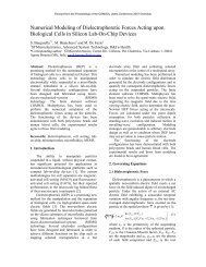
3D Simulation of the Thermal Response Test in a U ... - COMSOL.com

Presented at the COMSOL Conference 2009 Milan

Target
• Commonly used in GEOTHERMAL
applications to restore the equivalent values
of both the soil thermal conductivity (λ eq ) and
the borehole thermal resistance (Rb eq ).
• The estimation procedure is based on the
comparison of experimental TRT data with
the solution of the equations describing the
model’s behaviour (i.e. Line Source Model,
Cylinder Source Model).
To discuss the capability of the Thermal Response Test based on the
Line Source Model with regards to the characterization of borehole
energy storage systems in real conditions of non-linear and nonuniform
heat source.
Linda Schiavi – Comsol Conference 2009 2

3D transient conduction heat
transfer problem within the soil,
the borehole filling material
and the HDPE tubes is coupled
with the 1D convective
problem within the carrier fluid
Geothermal Energy Storage System’s Geometry
41080 prism meshing
elements
a) Radial meshing; b) Axial meshing
Linda Schiavi – Comsol Conference 2009 3

T
T
t
c p
r, z,0
T0
T
r
r
r
t
div
h
o
T
T
fluid
Initial condition
z,
t
T
r , z,
t
t
Boundary condition
Transient tri-dimensional heat transfer
conduction governed by the Fourier
equation is solved in the domain of the
soil, the filling material and the HDPE
tubes.
By assuming that the convection problem in both the tubes of the heat exchanger is
one-dimensional
A
T i
Ti
Ti
f
c
pf
u ho
T rt
, z,
t Ti
z,
t
t z
z, 0 T
0
Initial condition
Energy equation for the right-tube
downward fluid flow
A
T f
T
f
T
f
f
c
pf
u ho
T rt
, z,
t T
f
z,
t
t z
z, 0 T
0
Initial condition
Energy equation for the left-tube
upward fluid flow
Linda Schiavi – Comsol Conference 2009 4

The U-connection at the bottom of the pipe between the downward and
upward fluid is here modelled by imposing for z=H that the mean
temperature of the upward fluid equals the mean temperature of the
downward fluid:
Ti H , t T
f
H,
t
The condition of constant power supplied to the working fluid is implemented
by the periodic edge condition:
Ti 0, t Tf
0,
t
T
with T constant over the whole temporal domain.
Linda Schiavi – Comsol Conference 2009 5

Main input data for the tested cases
Working Fluid Mass Flowrate
0.1 kg/s
Fluid density 1000 kg/m 3
Fluid specific heat 4186 J/(kg K)
Inlet-Oulet Fluid temperature difference 3.6 K
Convective Coefficient (Dittus-Boelter) 1960 W/(m 2 K)
Soil density 1000 kg/m 3
Soil specific heat 2000 J/(kg K)
CASE A:
Soil thermal conductivity
2 W/(m K)
CASE B:
3 W/(m K)
Fill density 1000 kg/m 3
Fill specific heat 1000 J/(kg K)
Fill thermal conductivity 0.9 W/(m K)
HDPE density 950 kg/m 3
HDPE specific heat 1900 J/(kg K)
HDPE thermal conductivity 0.48 W/(m K)
Linda Schiavi – Comsol Conference 2009 6

LINE SOURCE MODEL:
Tf(t) =m+ k*ln(t)
where:
m= T0+ Q/(4 πλH) *(ln(4 α/rb2) -γ) + RbQ/H
k= Q/(4 πλH)
Temporal borehole temperature distribution at z=0
Average fluid temperature versus time for case A
Linda Schiavi – Comsol Conference 2009 7

Estimated thermal conductivity for case A
Estimated thermal conductivity for case B
The Line Source Model satisfactory predicts the thermal
conductivity of the soil, by restoring the parameter proper
value already in the first 30 hours.
Linda Schiavi – Comsol Conference 2009 8

Estimated borehole thermal resistance
• The two cases differ each other only for 1,5% for a variation of
50% of the soil thermal conductivity.
• They differ from the value numerically calculated in steady
state regime for less than 5% (R b =0.1625).
Linda Schiavi – Comsol Conference 2009 9

• The Line Source Model applied to the Thermal
Response Test represents a sufficiently
accurate approach also in the U-tube
configuration.
• The 3D approach appears necessary when
other more complex geometric configurations,
or other phenomena have to be considered.
Linda Schiavi – Comsol Conference 2009 10