Phase Diagram of the Two-Channel Kondo Lattice - APS Link ...

VOLUME 78, NUMBER 10 PHYSICAL REVIEW LETTERS 10MARCH 1997
Formalism and Simulation.—Metzner and Vollhardt
[13] provided a simplified method for solving such problems
in a nontrivial limit. They observed that the renormalizations
due to local two-particle interactions become
purely local for the coordination number tending to infinity.
In consequence, most standard lattice models may be
mapped onto the solution of an effective correlated impurity
coupled to a self-consistently determined bath or
medium (see [14] for further details and references).
We solve the effective impurity problem for Eq. (1)
by using the quantum Monte Carlo (QMC) algorithm of
Fye and Hirsch [15], modified for the two-channel Kondo
model [16]. We simulated the model for several fillings
N 0 , N # 1 and exchange interaction strengths J
J 0.75, 0.625, 0.5, 0.4. Error bars on the measured
quantities are less than 6% for the results presented
here. A sign problem encountered in the QMC process
prevented us from studying J $ 0.8 and N # 0.5 since
lower temperatures are required to access the physically
interesting regime.
The QMC simulation naturally produces both one- and
two-particle properties. The local spin susceptibility x L
was obtained by measuring the three-by-three matrix of
the local susceptibility, including both the Kondo spin and
conduction band spin fluctuations. x was then inverted to
calculate the associated irreducible vertex function and the
corresponding lattice susceptibility in the usual way [17].
The situation for the superconductivity is more complicated.
Only the two conduction channels contribute
to the pair-field susceptibility. We can then look
for pairing instabilities in singlet and triplet channels
for both spin and channel. Motivated by impurity
model results [5,6], we have restricted our attention to
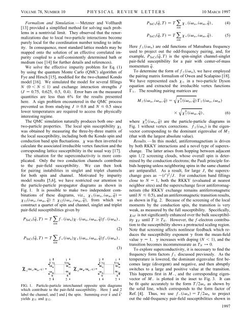
the particle-particle propagator diagrams as shown in
Fig. 1. It is possible to make two independent combinations
of these diagrams, viz., x 6 iv n , iv m , q
x 11 iv n , iv m , q 6x 12 iv n , iv m , q, from which we
construct a quartet of spin and channel, singlet and triplet
pair-field susceptibilities given by
P SsCs q, T T X nm
f 2 iv n x 2 iv n , iv m , qf 2 iv m ,
(2)
P StCt q, T T X f 1 iv n x 1 iv n , iv m , qf 1 iv m ,
nm
(3)
FIG. 1. Particle-particle interchannel opposite spin diagrams
which contribute to the pair-field susceptibility. Here 1 and 2
label the channel, and " and # the spin. Summing over k and k 0
yields x 11 and x 12 .
P StCs q, T T X nm
x 2 iv n , iv m , q , (4)
P SsCt q, T T X nm
x 1 iv n , iv m , q . (5)
Here f 6 iv n are odd functions of Matsubara frequency
used to project out the odd-frequency pairing, and, for
example, P SsCs q, T is the spin-singlet channel-singlet
pair-field susceptibility for a pair with center-of-mass
momentum q.
To determine the form of f 6 iv n , we have employed
the pairing matrix formalism of Owen and Scalapino [18].
We have represented each x 6 in a two-particle Dyson
equation and extracted the irreducible vertex functions
G 6 . The resulting pairing matrices are
q
M 6 iv n , iv m , q x6iv 0 n , q G 6 iv n , iv m
3
q
x 0 6iv m , q , (6)
where x6 0 iv n, q are the particle-particle diagrams in
Fig. 1 without vertex corrections. f 6 iv n is the eigenvector
corresponding to the dominant eigenvalue of M 6
(that with the largest absolute value).
Results.—In this model, antiferromagnetism is driven
by both RKKY interactions and a novel type of superexchange.
The latter arises from hopping between adjacent
spin 12 screening clouds, whose overall spin is determined
by the conduction electrons; the Pauli principle forbids
hopping unless neighboring spins in the same channel
are antiparallel. As a result, for large J, the superexchange
goes as t 2 J. For conduction band fillings
close to N 1, both the RKKY (evaluated at nearest
neighbor sites) and the superexchange favor antiferromagnetism
(the RKKY exchange remains antiferromagnetic
until N & 0.5), and an antiferromagnetic transition results,
as shown in Fig. 2. Because of the screening of the local
moments by the conduction spin, the transition is very
weak, as measured by the full susceptibility. Specifically,
x AF is not significantly enhanced over the bulk susceptibility
x F until T * T N . However, the f-electron contribution
to the susceptibility shows a protracted scaling region.
Note that screening affects nonlinear feedback which reduces
the susceptibility exponent g from the mean-field
value g 1. g increases with doping N , 1, and the
transition becomes incommensurate as T N ! 0.
To explore superconductivity, it is necessary to find the
frequency form factors f 6 discussed previously. As the
temperature is lowered, the dominant eigenvalue first becomes
large (divergent) and negative, and then abruptly
switches to a large and positive value at the transition.
This happens first in M 2 , and the corresponding eigenvector
of M 2 is plotted in the inset to Fig. 3. It can
be fit quite accurately to the form T2v n as shown by
the solid line, which corresponds to the form factor of
Ref. [4]. Thus, we use f 2 iv n T2v n to project
out the odd-frequency pair-field susceptibilities shown in
1997