Fault Detection and Diagnostics for Rooftop Air Conditioners

CALIFORNIA ENERGY 

COMMISSION 

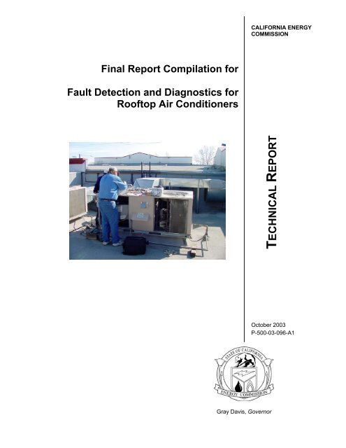
Final Report Compilation for 

Fault Detection and Diagnostics for 

Rooftop Air Conditioners 

TECHNICAL REPORT 

October 2003 

P-500-03-096-A1 

Gray Davis, Governor

CALIFORNIA 

ENERGY 

COMMISSION 

Prepared By: 

Architectural Energy Corporation 

Vernon A. Smith 

Boulder, CO 

Purdue University 

James Braun 

West Layfayette, IN 

CEC Contract No. 400-99-011 

Prepared For: 

Christopher Scruton 

Contract Manager 

Nancy Jenkins 

PIER Buildings Program Manager 

Terry Surles 

PIER Program Director 

Robert L. Therkelsen 

Executive Director 

DISCLAIMER 

This report was prepared as the result of work sponsored by the 

California Energy Commission. It does not necessarily represent 

the views of the Energy Commission, its employees or the State 

of California. The Energy Commission, the State of California, its 

employees, contractors and subcontractors make no warrant, 

express or implied, and assume no legal liability for the 

information in this report; nor does any party represent that the 

uses of this information will not infringe upon privately owned 

rights. This report has not been approved or disapproved by the 

California Energy Commission nor has the California Energy 

Commission passed upon the accuracy or adequacy of the 

information in this report. 

ii

Acknowledgements 

Jim Braun and Haorong Li with Purdue University conducted the research 

with support from Todd Rossi and Doug Dietrich with Field Diagnostic 

Services, Inc. David Jump with Nexant, Inc. and Lanny Ross with 

Newport Design Consultants provided field support. 

iii

Preface 

The Public Interest Energy Research (PIER) Program supports public interest 

energy research and development that will help improve the quality of life in 

California by bringing environmentally safe, affordable, and reliable energy 

services and products to the marketplace. 

The Program’s final report and its attachments are intended to provide a complete 

record of the objectives, methods, findings and accomplishments of the Energy 

Efficient and Affordable Commercial and Residential Buildings Program. This 

attachment is a compilation of reports from Project 2.1, Fault Detection and 

Diagnostics for Rooftop Air Conditioners, providing supplemental information to 

the final report (Commission publication #P500-03-096). The reports, and 

particularly the attachments, are highly applicable to architects, designers, 

contractors, building owners and operators, manufacturers, researchers, and the 

energy efficiency community. 

This document is one of 17 technical attachments to the final report, 

consolidating five research reports from Project 2.1: 

• Description of Field Test Sites (Feb 2003, rev.) 

• Description of FDD Modeling Approach For Normal 

Performance Expectation (Dec 2001) 

• Description And Evaluation Of An Improved FDD Method For 

Rooftop Air Conditioners (Aug 2002) 

• Decoupling-Based FDD Approach For Multiple Simultaneous 

Faults (June 2003) 

• Automated Fault Detection and Diagnostics of Rooftop Air 

Conditioners For California, Final Report and Economic 

Assessment (Aug 2003) 

The Buildings Program Area within the Public Interest Energy Research (PIER) 

Program produced this document as part of a multi-project programmatic 

contract (#400-99-011). The Buildings Program includes new and existing 

buildings in both the residential and the nonresidential sectors. The program 

seeks to decrease building energy use through research that will develop or 

improve energy-efficient technologies, strategies, tools, and building 

performance evaluation methods. 

For the final report, other attachments or reports produced within this contract, or 

to obtain more information on the PIER Program, please visit 

www.energy.ca.gov/pier/buildings or contact the Commission’s Publications 

Unit at 916-654-5200. The reports and attachments, as well as the individual 

research reports, are is also available at www.archenergy.com. 

iv

Abstract 

Project 2.1, Fault Detection and Diagnostics for Rooftop Air 

Conditioners. 

Packaged air conditioners are the most poorly maintained type of HVAC 

system. In California, they use about 54% of the HVAC energy in the 

commercial sector. The Purdue research team developed thermo-fluids 

based fault detection methods that can pinpoint five common maintenance 

problems. 

• This project was highly successful, resulting in a cost-effective method 

to detect simultaneous faults using only temperature sensors and 

models of normal operations. 

• Controllers that embed these diagnostics methods will save energy and 

maintenance costs by providing alerts only when maintenance is 

needed and giving the mechanic better information. 

• The historical data from the diagnostic system will also serve as a 

database for manufacturers to improve the reliability of components. 

This document is a compilation of five technical reports from the research. 

v

DESCRIPTION OF FIELD TEST SITES 

Revision for Walgreens Field Sites 

Deliverables 2.1.1a, 2.1.1b, and 3.1.1a 

Progress report submitted to: 


For the Building Energy Efficiency Program 

Sponsored by: 

California Energy Commission 

Submitted By: 


Principal Investigator: 

Research Assistants: 

James Braun, Ph.D., P.E. 

Tom Lawrence, P.E. 

Kevin Mercer 

Haorong Li 

April 2001 

Revision February 2003 

Mechanical Engineering 

1077 Ray W. Herrick Laboratories 

West Lafayette, IN 47907-1077 

(765) 496-6008 

(765) 494-0787 (fax)

TABLE OF CONTENTS 

LIST OF TABLES 

LIST OF FIGURES 

Page 

ii 

iii 

1. INTRODUCTION 1 

1.1 Purdue Research Projects under this Program 1 

2.2 Related Reports 1 

2. SELECTION OF FIELD TEST SITES 3 

2.1 Criteria for selection of the building and climate types 3 

2.2 California climate types 4 

2.3 Method for selecting sites 4 

3. DESCRIPTION OF FIELD TEST SITES 7 

3.1 Modular School Rooms 9 

3.2 Fast Food Restaurants 17 

3.3 Retail Stores 36 

4. TESTING PLAN 39 

i


Page 

1 – Data List for Modular School Room Field Test Sites 12 

2 - Data List for Inland Restaurant Field Test Sites (Watt Avenue and Castro Valley) 23 

3 - Data List for Inland Restaurant Field Test Sites (Bradshaw Road and Milpitas) 26 

ii


Page 

1 – Field Test Sites Data Collection and Communication Overview 8 

iii

1. INTRODUCTION 

Purdue University is under contract to Architectural Energy Corporation on behalf of the 

California Energy Commission (CEC) to conduct several research projects. This work is 

being done under the Building Energy Efficiency Program as part of the CEC’s Public 

Interest Energy Research (PIER) Program. 

1.1 Purdue Research Projects under this Program 

The work at Purdue is focused on four specific projects and is being coordinated under 

the direction of Dr. James Braun, P.E. Each project covers different technologies or 

concepts that have shown promise for improving energy efficiency in building heating, 

ventilation and air conditioning (HVAC) systems. Specifically, the four projects that 

Purdue is working on include evaluations and studies of the following. (1) fault detection 

and diagnostics (FDD) of rooftop air conditioning units (Project 2.1); (2) demand 

controlled ventilation (DCV) assessment (Project 3.1); (3) assessment and field testing of 

ventilation recovery heat pumps (Project 4.2); and (4) night ventilation with building 

thermal mass (Project 3.2). 

The first three of these projects are currently active, with the Project 3.2 scheduled to 

start in September of 2001. All four of the projects involve both theoretical analysis and 

field demonstration and evaluation. This report describes the field test sites selected for 

use in projects 2.1 and 3.1. Monitoring equipment has been installed at modular school 

room and restaurant field sites in Northern California. We have an agreement with the 

Walgreens Company to allow use of retail store sites in the Los Angeles metropolitan 

area, and installation is expected to being in August of 2001. An update to this report 

will be issued when the retail store installations are finalized. 

1.2 Related Reports 

This report describes the field test sites selected for use with the CEC PIER project. 

Other related reports submitted in parallel with this report are: (1) “Description of 

Laboratory Setup” and (2) “Modeling And Testing Strategies for Evaluating Ventilation 

Load Reduction Technologies. 

1

The report “Description of Laboratory Setup” provides a description of the York rooftop 

unit and Honeywell Demand Controlled Ventilation system that are installed outside the 

Purdue Herrick Laboratory and the instrumentation used for monitoring the setup.. This 

setup follows closely the field site setups in California. The instrumentation includes 

measurement of system temperatures, pressures, relative humidities and carbon dioxide 

concentrations. The Laboratory Setup report covers in detail the setup and operation of 

the Virtual Mechanic hardware and ACRx ServiceTool Suite of monitoring software, 

both provided by Field Diagnostic Services. Finally, the report describes the general 

process for collecting and retrieving data downloaded from the field test sites. 

The “Ventilation Strategy Analysis” report presents an overview of the modeling 

approach and input data to be used in evaluating the energy savings associated with 

several ventilation load reduction technologies. In addition, an overview of the 

preliminary test plan and field site monitoring setup for the heat pump heat recovery unit 

is given. 

2

2. SELECTION OF FIELD TEST SITES 

Projects 2.1 and 3.1 involve the use of 12 common field sites for evaluation of FDD and 

demand-controlled ventilation. In these two projects, field performance data will be 

obtained from heating/cooling units. Three different building types are being utilized in 

two different climate zones. 

2.1 Criteria for selection of the building types 

All of the Purdue projects are focused on small commercial buildings that utilize 

packaged air conditioning and heating equipment. The criteria used for selecting the 

types of buildings to include as field test sites focused on the typical building occupancy 

schedule, the building size and typical HVAC system installed, and the ability to identify 

multiple sites of similar design and construction within the same climate region. To 

reduce costs, the same test buildings are being used for the field studies in Projects 2.1 

(fault detection and diagnostics) and 3.5 (demand-controlled ventilation). Earlier studies 

on demand-controlled ventilation indicated that the greatest benefits (in terms of energy 

savings) are possible with buildings that have variable occupancy schedules. Thus, the 

three building types selected for the field test sites are smaller retail stores, restaurants 

and schools. For each type of building, two nearly identical sites will be used in two 

different climates. This will allow comparative analysis of the energy savings associated 

with demand-controlled ventilation in terms of building type and climate. The fault 

detection and diagnostics project is focused strictly on small commercial packaged air 

conditioning units, so the field sites provide a range of equipment for demonstration and 

evaluation of this technology. A single site will be used to demonstrate a heat pump heat 

recovery unit. However, the data obtained from the demand-controlled ventilation sites 

can also be used to estimate savings for the heat pump heat recovery unit if it were 

installed in these additional sites. 

A large number of modular schoolrooms are installed throughout the state of California. 

These rooms are all very similar in design and construction, and all typically use wall 

3

mounted heat pumps for heating and cooling. One advantage of the modular schoolroom 

for this study is that essentially identical rooms can be monitored side-by-side. 

For the restaurant building type, the systems used to condition the children’s play areas 

that are common in many fast food chains will be monitored. These rooms typically are 

self-contained, or nearly so, and only require one or two rooftop units for cooling and 

heating. By monitoring only the play areas in these restaurants, the study can gather data 

on spaces that have the greatest variability in occupancy, and also will eliminate the 

effects of the kitchen area and its associated ventilation systems. 

The third building type selected is a small retail store. Small retail stores can have an 

extremely wide variation in occupancy patterns. Chain stores were considered for the 

study since essentially identical buildings can be found. 

2.2 California Climate Types 

Although California has a wide range of climate types, much of the state can be 

characterized as a Mediterranean climate. This climate type experiences warm, dry 

summers and temperate moist winters. The state also includes desert regions in southern 

California (such as Palm Springs) and coastal regions. The specific climate type for a 

given locality may vary significantly within a small distance due to the influence of 

factors such as topology and the proximity to the ocean. Some of the best examples of 

these variations occur in the San Francisco Bay area where the distance of just a few 

miles can lead to significant variations in rainfall patterns and sky conditions 

2.3 Method for selecting sites 

It is not possible within the scope of this project to evaluate the new technologies for all 

possible climate regions in California using field data. However, it will be possible to 

perform more extensive evaluations through simulation. For the field studies, 

representative buildings were selected in two different macroclimate types (coastal and 

4

inland). In addition, some of the selected sites are in northern California and some are in 

southern California, which gives as wide a range of location and climate type as practical 

within the context of these projects. The inland sites vary from the Mediterranean 

climate type of the Central Valley around Sacramento to the desert regions around Palm 

Springs. Although it was not possible to have field sites for all technologies in all climate 

regions, the areas selected for study represent those with the greatest concentration of 

population and commercial development. 

Before the projects officially started, contacts were made with the owners of potential 

building sites within the school, restaurant and retail store categories. The identification 

of sites has been a time consuming process that has required the help of several of the 

participating organizations, including Honeywell, Schiller Associates, Carrier 

Corporation, Southern California Edison, and Architectural Energy Corporation. 

The first buildings identified were schools. During the summer of 2000, contacts were 

made and meetings held with representatives of the Oakland Unified School District and 

the Woodland Joint Unified School District. Woodland is approximately 20 miles west 

of Sacramento and represents an inland climate type. The monitoring systems were 

installed at two rooms located side-by-side at each of the two school districts in 

December of 2000. More details on these sites are contained later in this report. 

The restaurant building type is represented by two franchisee owned McDonald’s stores 

in the Sacramento area and by two corporate owned stores on the southeastern San 

Francisco Bay area. These stores have PlayPlace areas with similar construction and 

HVAC system installations, although it was not possible to find stores with identical 

design and sun orientation. Sun orientation can be particularly important for the 

PlayPlace areas, since they typically include a large percentage of glass area. 

Monitoring equipment was installed in the Sacramento McDonalds during the middle of 

March, 2001. In the San Francisco Bay Area, a representative of McDonalds corporate 

office identified two stores for inclusion in our study that will be the best fit for our 

needs. Monitoring equipment were installed in May of 2001 at these two stores. More 

details on these sites are also given in the later sections of this report. 

5

The retail stores are in Southern California. The Walgreens corporation has agreed to our 

using their stores as part of this program. Monitoring systems are installed at stores 

located in Rialto (near Riverside) and Anaheim. The Rialto store is located in a near 

desert climate, while Anaheim is a more coastal climate type. 

6

3. DESCRIPTION OF FIELD TEST SITES 

Figure 1 presents a general overview of how data are monitored and collected from the 

field sites. Proprietary equipment from Honeywell controls ventilation dampers using 

economizer and demand-control ventilation algorithms. The Honeywell controller 

incorporates sensors to measure ambient temperature and humidity, return air 

temperature and carbon-dioxide concentration, and mixed air temperature. Additional 

sensors are installed to monitor other air state variables, refrigerant states, power 

consumption, and operational status. The primary data acquisition is accomplished using 

hardware from Field Diagnostics Services (FDS) called the Virtual Mechanic (VM). The 

VM communicates with the Honeywell controller across an RS485 network to obtain 

sensor information and to change control strategies. The additional sensors are wired 

directly to the VM. Data are sampled at approximately 5-minute intervals and are stored 

in the VM. For some field sites, multiple VMs are employed for multiple packaged air 

conditioners. Data are downloaded each day using cell phones connected to the master 

Virtual Mechanic at each test site. 

A detailed description of the field test sites is provided in the following subsections. 

Some of the detailed technical information needed to simulate the performance of the 

different technologies for these buildings will be compiled later in the project. This 

section contains information on the following test sites: 

• Modular School Rooms – Inland Climate Type 

• Modular School Rooms – Coastal Climate Type 

• Fast Food Restaurants – Inland Climate Type 

• Fast Food Restaurants – Coastal Climate Type 

• Retail Stores – Inland Climate 

• Retail Stores – Coastal Climate 

7

Figure 1 – Field Test Sites Data Collection and Communication Overview 

Analog Data Direct Input to Virtual Mechanic 

Suction line P, Stage 1 Suction line P, Stage 2 

Liq. line P Stage 1 Liq. line P, Stage 2 

Suction line T, Stage 1 Suction line T, Stage 2 

Discharge T, Stage 1 Discharge T, Stage 2 

Liq. T before filter, 1 Liq. T before filter, 2 

Liq. T after filter, 1 Liq. T after filter, 2 

Cond. outlet air T, Stg 1 Cond. outlet air T, Stg 2 

Mixed air %RH Supply air T 

Supply air %RH SPARE 

Evap. T, Stage 1 Evap. T, Stage 2 

Cond. T, Stage 1 Cond. T, Stage 2 

SPARE 

SPARE 

Data Points from Rooftop 

Unit Power Module 

• Current transducer, #1 



• Voltage transducer, #1 



• Alternate: Power meters 

Digital Data Channels 

• Supply fan contact 

• Low V control signal, compr. 1 

• Low V control signal, compr. 2 

• Gas valve contact, stage 1 

• Gas valve contact, stage 2 

REMOTE DATA 

ACCESS BY FDS 

VIA PHONE, 

ACCESSIBLE 

ON WEB FOR 

DATA 

ANALYSIS 

MULTIPLE VIRTUAL 

MECHANIC UNITS CONNECTED 

IN A LOCAL NETWORK. 

(ONE FOR EACH ROOFTOP 

UNIT) 

FDS Virtual 

Mechanic 

UNIT #1 

RS 485 LOCAL 

AREA NETWORK 

Honeywell Economizer/Demand 

Controlled Ventilation (DCV) Controller 

• Ambient T 

• Ambient %RH 

• Mixed air T 

• Return air T 

• Return air CO 2 

FDS Virtual 

Mechanic 

UNIT #n 

FDS Virtual 

Mechanic 

UNIT #2 

Data Points Direct Input 

to DCV Controller 

Rooftop Unit #n Rooftop Unit #2 

8

BUILDING TYPE: 

Modular School Rooms 

Inland Climate Locations 

ADDRESS: 

Gibson Elementary School 

312 Gibson Road 

Woodland, CA 95695 

(530) 662-3944 

EQUIPMENT INSTALLATION DATE: December 14-19, 2000 

CELL PHONE NUMBER: (765) 427-0311 

DETAILED BUILDING DESCRIPTION: 

Floor Area 

Building Orientation 

Wall Construction 

20 feet by 40 feet (800 sq. ft.) 

East – West 

Walls are 2x4 stud construction with R-11 insulation. 

Internal walls have ¾” vinyl covered fiberboard over 

5 / 8 ” gypsum wallboard. 

Windows/ Shading 

Wood panel exterior with no windows on south or 

north sides. East and west sides have one 4’ x 8’ 

window, with door on east side. Two-foot overhang 

on west wall and three-foot overhang on east wall 

entrance area. 

Windows are double-pane with ¼” air gap. 

Roof/Ceiling Construction Flat roof with reflective paint coating. Roof has R-19 

insulation. Interior drop ceiling is 8’ above occupied 

space with t-bar 18” below the roof. 

Floor 

Lighting 

Other Loads and 

Equipment 

Occupancy Patterns 

Crawl space below is ventilated with R-11 insulation 

below floor. 

10 sets of fluorescent lights, 120 W each with 

magnetic ballast. 

One desktop computer and one small refrigerator. 

8:30 am to 3:00 pm weekdays. Usually one or two 

hours on Saturday mornings. 

The rooms are occupied by 15-20 small children per 

room, plus teacher. (These are kindergarten – first 

grade rooms.) 

9

Gibson School (Cont’d) 

Woodland School Site – 

Rear View Looking East 

Woodland School Site – 

Front View Looking West 

Each building (modular school room) has its own packaged air conditioner/heat pump. 

Two side-by-side units have been retrofit with the Honeywell economizer and demand 

control ventilation system and fully instrumented. Two VMs are networked together 

with one of units linked to a cell phone. The heat pump units were originally set up for 

fixed percentage of outdoor air, and did not have outdoor air flow control dampers. It 

was estimated that, based on the installation configuration, the airflow control was set up 

for approximately 15% outdoor air at these sites before the retrofit. 

10

HEATING / AIR CONDITIONING EQUIPMENT: 

Each building (room) has a sidewall-mounted heat pump as described in the table below. 

Manufacturer 

Bard Manufacturing 

Model WH 421-A 

Nominal Cooling Capacity 

Number of Stages 1 

3½ Tons 

SEER / HSPF 10.0 / 6.8 

Supplemental Heating 

Capacity 

Electrical 

10 kW nominal electric resistance heater. 

Single phase, 220 V 

Supply Fan Rating 1400 cfm @ 0.3” 

TEST INSTRUMENTATION: 

Table 1 lists the input data channels used at the modular schoolrooms. The same data list 

is used at both the Woodland and Oakland school sites. 

11

Table 1 – Data List for Modular School Room Field Test Sites 

Channel # Data Point 

Power Transducer Channels 

1 Unit voltage 

2 Compressor 1 voltage 

3 Common 

4 Unit total current 

5 Compressor 1 current 

6 - 8 Spare - Not Used 

Other Analog Input Data 

9 Suction line pressure, Stage 1 

10 Liquid line pressure, Stage 1 

11 - 14 Spare - Not Used 

15 Mixed air temperature 

16 Return air temperature 

17 Supply air temperature, before heater 

18 Supply air temperature, after heater 

19 Condenser inlet air temperature 

20 Condenser outlet air temperature 

21 Suction line temperature, Stage 1 

22 Discharge line temperature, Stage 1 

23 SPARE - Used as additional ambient T 

24 SPARE - Used as additional ambient T 

25 Evaporation temperature, Stage 1 

26 Condensation temperature, Stage 1 

27- 32 Spare - Not Used 

Calculated Data Channels 

33-50 NOT USED 

51 Honeywell DCV indoor (and outdoor) CO2 conc. 

52 Honeywell DCV mixed air temperature 

53 Honeywell DCV return air temperature 

54 Honeywell DCV return / outdoor humidity 

55 Honeywell DCV outdoor air temp & damper position 

56 Honeywell DCV minimum damper position 

57 superheat, stage 1 

58 subcooling, stage 1 

59 evaporating temperature, stage 1 

60 condensing temperature, stage 1 

61 condensing temperature over ambient (CT-AIC), stage 1 






12

Table 1 – Data List for Inland Modular School Room Field Test Site (Cont’d) 

Channel Data Point 

67 evaporator temperature difference (RA-SA) 

68 NOT USED 

69 NOT USED 

70 unit power (kW) 

71 unit KWh 

72 unit MWh 

73 compressor 1 power (kW) 

74 compressor 1 KWh 

75 compressor 1 MWh 




79 digital input 1, supply fan, run time (8 hours) 

80 digital input 1, supply fan, run time (seconds) 

81 digital input 2, cooling 1, run time (8 hours) 

82 digital input 2, cooling 1, run time (seconds) 



85 digital input 4, heat 1, run time (8 hours) 

86 digital input 4, heat 1, run time (seconds) 



89 digital input 6 run time (8 hours) 

90 digital input 6 run time (seconds) 

91 time since reset accumulators (8 hours) 

92 time since reset accumulators (seconds) 

93 up time (8 hours) 

94 up time (seconds) 

95 board temperature (F) 

96 board battery voltage (V) 

Digital Channels 

1 Supply fan contact (fan on / fan off) 

2 Low voltage control signal for compressor contact 

3 Spare 

4 Heat on 

5 Electric heat 

6 

13


Modular School Rooms 

Coastal Climate Location 

ADDRESS: 

Fremont High School 

4610 Foothill Blvd. 

Oakland, CA 

(510) 879-3020 

EQUIPMENT INSTALLATION DATE: December 19-21, 2000 

CELL PHONE NUMBER: (765) 427-0325 

DEtAILED DESCRIPTION: 

Floor Area 



20 feet by 40 feet (800 sq. ft.) 

East – West 

Walls are 2x4 stud construction with R-11 insulation. 

Internal walls have ¾” vinyl covered fiberboard over 

5 / 8 ” gypsum wallboard. 


Wood panel exterior with no windows on south or 

north sides. East and west sides have one 4’ x 8’ 

window, with door on east side. Two-foot overhang 

on west wall and three-foot overhang on east wall 

entrance area. 

Windows are double-pane with ¼” air gap. 

Roof/Ceiling Construction Flat roof with reflective paint coating. Roof has R-19 

insulation. Interior drop ceiling is 8’ above occupied 

space with t-bar 18” below the roof. 

Floor 

Lighting 


Equipment 


Crawl space below is ventilated with R-11 insulation 

below floor. 

Approximately 10 sets of fluorescent lights, 120 W 

each with magnetic ballast. 

One desktop computer. (To be verified) 

8:30 am to 3:00 pm weekdays. 

The rooms are occupied by 15-20 high school 

students per classroom. 

14

Fremont High School (Cont’d) 

Oakland School Site (Fremont High 

School) - View Looking Along North Walls 

Each building (modular school room) has its own packaged air conditioner/heat pump. 

Two side-by-side units have been retrofit with the Honeywell economizer and demand 

control ventilation system and fully instrumented. Two VMs are networked together 

with one of units linked to a cell phone. The heat pump units were originally set up for 

fixed percentage of outdoor air, and did not have outdoor air flow control dampers. It 

was estimated that, based on the installation configuration, the airflow control was set up 

for approximately 15% outdoor air at these sites before the retrofit. 

15


Each building (room) has a sidewall-mounted heat pump manufactured by Bard 

Industries, Model WH 421A. These are the same units as used at the Woodland school 

site. The units are contained within a fenced off area on the north end of the buildings. 


3½ Tons 

SEER / HSPF 10.0 / 6.8 

Heating Capacity 

Electrical 

10 kW nominal electric resistance heater. Note: The 

electrical resistance heaters are not functioning for 

these rooms. 

Single phase, 220 V 

Supply Fan Performance 1400 cfm @ 0.3” 


The Fremont school site uses the same data point list given in Table 1 for the Woodland 

schools. 

16


Fast Food Restaurants 

Inland Climate Locations 

ADDRESS: 

McDonalds Restaurant 

2434 Watt Ave. 

Sacramento, CA 95821 

(916) 971-0244 

3560 Bradshaw Road 

Sacramento, CA 95827 

(916) 361-8186 

CONTACT: 

Mike Godlove (Owner) 

2508 Garfield Ave 

Carmichael, CA 95608 

(916) 483-6065 

EQUIPMENT INSTALLATION DATE: March 12-14, 2001 

CELL PHONE NUMBERS: (765) 427-7714 and 427-7919 

DEtAILED DESCRIPTION: 

Equipment at two nearly identical McDonald’s PlayPlaces in Sacramento have been 

retrofit with the Honeywell economizer and demand control ventilation system and fully 

instrumented. Each system has its own dedicated VM with a cell phone for data 

transmission. The Watt Avenue site has a slightly smaller floor area (approximately 20 

square feet less take from two corners). The following subsections give some details on 

the building construction and operation. Additional details will be obtained later. 

17

Sacramento Area McDonalds PlayPlace Construction (Watt Avenue and Bradshaw 

Road) 

Floor Area 




Roof/Ceiling Construction 

Floor 

Lighting 


Equipment 


Approximately 20 feet by 30 feet (600 sq. ft.) that is 

for the most part isolated from the dining and 

cooking areas. 

Primary axis for this room is North - South. 

Major glass surfaces on the East and South walls. 

West face is interior wall shared with the dining area. 

“Stucco” exterior covering. 

Major glass surfaces on the East and South walls. 

West face is interior wall shared with the dining area. 

Some window area on North wall. No exterior 

shading. Windows are tinted with double pane, ¼” 

air gap construction. 

Flat roof with light colored asphalt coating. 

Tile on slab construction. 

Approximately six sets of fluorescent lights, with 

four bulbs each with magnetic ballast. 

Some air exchange with dining area and outdoor air 

via door in the common vestibule. 

Ceiling fans keep air in motion. 

PlayPlace hours are: 9 am to 9:30 pm. 

Occupancy varies from 0 to a maximum of 

approximately 40. 

18

Watt Avenue (Sacramento Area) McDonalds PlayPlace Pictures 

Watt Avenue McDonalds – 

View Looking Southwest 

Interior view of Watt Avenue 

McDonalds PlayPlace Area showing 

location of return air and supply air 

ducts. 

Watt Avenue McDonalds – 

Rooftop Units Undergoing Equipment Installation 

19

Bradshaw Road (Sacramento Area) McDonalds PlayPlace Pictures 

Interior view of Bradshaw Road McDonalds 

PlayPlace Area 

Bradshaw Road McDonalds – 

View Looking Northwest 

Bradshaw Road McDonalds – 

Rooftop Units Undergoing Equipment Installation 


Each PlayPlace uses rooftop-mounted units for providing heating, cooling and ventilation 

air to the room. The two sites differ in the number of rooftop units used, with the Watt 

Avenue building using one two-stage unit and the Bradshaw Road building using two 

smaller single-stage units. According to York International's regional support 

representative, the units are custom designed for supply to McDonalds Corporation for 

the PlayPlace areas. The following tables describe the units used at each site. Since they 

20

are custom designs, published performance ratings and other technical details were not 

readily available. This information will be obtained later. 

Watt Avenue 

Manufacturer 

York International 

Model 

D3CG120N20025MKD 

Nominal Cooling Capacity 10 Tons 


SEER / HSPF 

TBD 


200,000 Btu/hr nominal output 

Electrical 

Three phase, 220 V 

Supply Fan Performance 4,000 cfm manufacture rated 

Bradshaw Road 

Manufacturer 


Model 

D1CG072N07925ECC 



SEER / HSPF 

TBD 



Electrical 


Supply Fan Performance 2,400 cfm manufacture rated (each) 

21


Tables 2 and 3 list the data channels used at the restaurants. A slightly different list is 

required for each site since the HVAC equipment setup is different. In particular, the 

Watt Avenue site has one larger (10 ton) unit with 2-stage cooling to condition the entire 

room. The Bradshaw Road site, on the other hand, has two smaller (6 ton) single-stage 

cooling units operating in parallel. Instrumentation for fault detection and diagnostics 

and monitoring was set-up for one rooftop unit per site, as originally planned in the 

project proposal stage. Therefore, one unit at the Bradshaw Road site was fully 

instrumented for both FDD and DCV purposes, while the second unit was instrumented 

only for the purposes of collecting data for the DCV project. The Watt Avenue site has 

only one rooftop unit and was fully instrumented according to the standard data list. All 

data will be collected using one Virtual Mechanic at each site. 

22

Table 2 – Data List for Inland Restaurant Field Test Site (Watt Avenue) 


SENSOR CHANNELS 


1 Unit voltage 



4 Unit total current 




7 SPARE - Not used 



10 Discharge pressure, Stage 1 


12 Discharge pressure, Stage 2 



15 Mixed air temperature 

16 Return air temperature 

17 Supply air temperature, before heater 

18 Supply air temperature, after heater 

19 Condenser inlet air temperature 

20 Condenser outlet air temperature 



23 Liquid line temperature before filter/drier, Stage 1 

24 Liquid line temperature after filter/drier, Stage 1 





29 Liquid line temperature before filter/drier, Stage 2 

30 Liquid line temperature after filter/drier, Stage 2 



Calculated Data Channels 







23

Table 2 – Data List for Inland Restaurant Field Test Site (Watt Avenue) – Cont’d 













67 evaporator temperature difference (RA-SA) 

68 NOT USED 

69 NOT USED 


71 unit KWh 

72 unit MWh 

























24

Table 2 – Data List for Inland Restaurant Field Test Site (Watt Avenue) – Cont’d 


1 Supply fan contact (fan om / fan off) 

2 Low voltage control signal for compressor 1 contact 

3 Low voltage control signal for compressor 2 contact 

4 Heating 1 

5 Heating 2 

6 

25

Table 3 – Data List for Inland Restaurant Field Test Site (Bradshaw Road) 


SENSOR CHANNELS 


1 Unit 1 input voltage 

2 Compressor voltage, Unit 1 

3 Unit 2 input voltage 

4 Unit 1 total current 

5 Compressor current, Unit 1 

6 Unit 2 total current 




9 Suction line pressure, Unit 1 

10 Discharge pressure, Unit 1 





15 Mixed air temperature - Unit 1 

16 Return air temperature - Unit 1 

17 Supply air temperature, before heater - Unit 1 

18 Supply air temperature, after heater - Unit 1 

19 Condenser inlet air temperature - Unit 1 

20 Condenser outlet air temperature - Unit 1 

21 Suction line temperature - Unit 1 

22 Discharge line temperature - Unit 1 

23 Liquid line temperature before filter/drier - Unit 1 

24 Liquid line temperature after filter/drier - Unit 1 

25 Evaporation temperature - Unit 1 

26 Condensation temperature - Unit 1 



29 Mixed air temperature - Unit 2 

30 Mixed air humidity - Unit 2 

31 Supply air temperature - Unit 2 

32 Supply air humidity - Unit 2 

CALCULATED DATA CHANNELS 







26

Table 3 – Data List for Inland Restaurant Field Test Site (Bradshaw Road) – Cont’d 








62 NOT USED 

63 NOT USED 

64 NOT USED 

65 NOT USED 

66 NOT USED 

67 NOT USED 

68 NOT USED 

69 NOT USED 


71 unit KWh 

72 unit MWh 

























27

Table 3 – Data List for Inland Restaurant Field Test Site (Bradshaw Road) – Cont’d 


1 Supply fan contact (fan om / fan off) 

2 Low voltage control signal for compressor contact 

3 Spare 

4 Heating 

5 Spare 

6 

28


Fast Food Restaurants 

Coastal Climate Locations 

ADDRESS: 

99 N. Milpitas Blvd. 

Milpitas, CA 95035 

(408) 263-0181 

1620 Storbridge Ave. 

Castro Valley, CA 94546 

(510) 537-9566 

CONTACT: 

Paul Martin 

(408) 422-2339 

EQUIPMENT INSTALLATION DATE: May 2001 

CELL PHONE NUMBERS: (765) 427-2988 

(765) 427-3052 

DETAILED DESCRIPTION: 

The PlayPlace areas at these two sites are not as close in design and orientation as are the 

two Sacramento sites. This is a compromise in order to get two sites that are reasonably 

close together and in a similar coastal climate zone. Both restaurants are located south of 

Oakland on the east edge of the San Francisco Bay and have a floor space of around 1300 

square feet, which is larger than the PlayPlace areas at the two Sacramento stores. The 

Castro Valley restaurant is oriented with its main glass area facing west. The Milpitas 

store, however, contains a larger glass area and is oriented facing north. The following 

subsections contain some descriptions of the room construction and heating/cooling 

equipment for these two coast climate restaurant sites. Additional details of the 

construction and building operation will be obtained later. 

29

Castro Valley (San Francisco Bay Area) McDonalds PlayPlace Construction 

Floor Area 





Floor 

Lighting 


Equipment 


Approximately 26 feet by 50 feet (1300 sq. ft.) that is 

isolated from the dining and cooking areas by an 

interior glass wall with two doors. 

Primary axis for this room is northwest - southeast. 

The long axis glass surface area faces southwest, with 

the smaller sides facing northwest and southeast. 

Northeast wall is interior wall shared with the dining 

area. 


Windows are tinted with double pane, ¼” air gap 

construction. Overhang of 24” at top that provides 

minimal shading. 

Total glass area of about 490 sq. ft. on southwest wall 

and 195 sq. ft. each on the northwest and southeast 

walls. 



Total of 26 fixtures of 48” fluorescent lights, with 

four bulbs each with magnetic ballast. Several had 

missing bulbs, only approximately 80% of bulbs in 

place. 

One TV and four video games. 


PlayPlace operating hours are 9am – 9pm. 

During visit on a Sunday afternoon, occupied by 

approximately 70 children and adults. 

30

Milpitas (San Francisco Bay Area) McDonalds PlayPlace Construction 

Floor Area 





Floor 

Lighting 


Equipment 


Approximately 24 feet by 50 feet with 6’ by 6’ corner 

that shares internal wall with kitchen storage. Total 

floor is approximately 1170 sq. ft. Zone is isolated 

from the dining and cooking areas by an interior glass 

wall with two doors. 

Primary axis for this room is east - west. 

The long axis glass surface area faces north, with the 

smaller sides facing west and east. South wall is 

interior wall shared with the dining area. 


Windows are tinted with double pane, ¼” air gap 

construction. Overhang of 24” at top that provides 

minimal shading. 

Exterior walls are essentially floor to ceiling covered 

in glass. Total glass area of about 1000 sq. ft. on 

north wall, 480 sq. ft. on the east wall and 360 sq. ft. 

on the west wall. 



Total of 19 fixtures of 48” fluorescent lights, with 

four bulbs each with magnetic ballast. 

No TVs or video games. 


PlayPlace operating hours are 8am – 9pm. 

31

Castro Valley McDonalds PlayPlace Pictures 

Interior view of Castro Valley McDonalds 

PlayPlace Area. 

Castro Valley McDonalds – 

View Looking Southeast 

Castro Valley McDonalds PlayPlace Area. 

York Rooftop Unit 

32

Milpitas McDonalds PlayPlace Pictures 

Milpitas McDonalds – 

View Looking Southeast 

Interior view of Milpitas McDonalds 

PlayPlace Area (NW Corner) 

Milpitas McDonalds PlayPlace Area. 

Two York Rooftop Units 


Each building (room) uses rooftop-mounted units for providing heating, cooling and 

ventilation air to the room. The two sites differ in the number of rooftop units used. Just 

like the two restaurants in Sacramento, one restaurant uses one two-stage York rooftop 

unit (Castro Valley) and the other (Milpitas) uses two smaller single-stage units. The 

units are of the same series that were designed and built specifically for the McDonalds 

PlayPlace areas. The following tables describe the units used at each site. Since they are 

33

more or less custom design, published performance ratings and other technical details 

were not readily available. 

Castro Valley 

Manufacturer 


Model 

D4CG150N16525MDB 



SEER / HSPF 

TBD 



Electrical 


Supply Fan Performance 4,000 cfm manufacture rated 

Milpitas 

Manufacturer 


Model 

D1CG072N09925C 



SEER / HSPF 

TBD 



Electrical 


Supply Fan Performance 2,400 cfm manufacture rated (each) 

34


Similar test instrumentation will be used as for the Sacramento McDonalds. The system 

at the restaurant with only one rooftop unit (Castro Valley) will be fully instrumented for 

both FDD and DCV studies, like the Watt Avenue site in Sacramento. The data list is 

presented in Table 2. The Milpitas site is analogous to the Bradshaw Road store in 

Sacramento, whereby one unit will be fully instrumented for both FDD and DCV 

purposes, while the second unit will be instrumented only for the purposes of collecting 

data for the DCV project. Table 3 provides this data list. All data will be collected using 

one VM at each site. 

35


Retail Store 

ADDRESS: 

Inland Climate Location 

Contact: 

Coastal Climate Location 

Contact: 

Walgreens 

550 S. Riverside 

Rialto, CA 

Gabriel Reyes (Store Manager) 

(709) 874-6600 

Walgreens 

946 S. Brookhurst 

Anaheim, CA 

Lee Anderson (Store Manager) 

(714) 520-5444 

EQUIPMENT INSTALLATION DATES: 

Rialto Store: VM Monitoring Equipment: August 1-5, 2001 

Functioning Honeywell Controls: June, 2002 

Anaheim Store: VM Monitoring Equipment: June, 2002 

Functioning Honeywell Controls: Fall 2002 

CELL PHONE NUMBERS: Dedicated land phone lines were installed in August 

2002 to replace the cell phone arrangement. 

DETAILED BUILDING DESCRIPTION: Rialto Store (Common Design) 

Floor Area 




100 feet by 90 feet (9,000 sq. ft.) in retail store space, 

40 feet by 20 feet in the pharmacy. An additional 35 

feet by 90 feet of backroom storage and 20 feet by 

100 feet for office and equipment that is not part of 

the DCV study. 

Generally north - south, with front door on northeast 

corner. 

Brick and stucco exterior. 

A total of 20 windows on the two exterior walls to 

the retail store area. Windows are 5 feet by 8 feet, 

tinted, double-pane with ¼” air gap. Windows are 

on the east and north walls. 

A five-foot overhang covers the sidewalk and shades 

the exterior windows. 

36


Floor 

Flat roof with light store coating. 

Floor tiles over concrete slab. 

Lighting Retail store has total of 170 fixtures with 2 bulbs, 8- 

foot long fluorescent lights. 


Equipment 


Pharmacy has 33 fixtures of 2 bulb, four-foot long 

fixtures. 

Refrigerated drink and food open to store, 25 feet 

linear feet. 

Freezer section with doors, 20 feet long. 

Photo processing machine plus two cash registers. 

Store hours are 8 am to 10 pm, seven days a week. 


Four rooftop heat pumps condition the retail store space and one additional unit is 

dedicated to the pharmacy area. A separate unit is installed at the store to condition the 

storage room, but since this is an isolated area not normally occupied, it is not part of the 

DCV installation study. The rooftop units are manufactured by Trane. 

Manufacturer 

Model 



SEER / HSPF 

Electrical 

Supply Fan Performance 

Trane 

WFD090C30BBC - Retail Store 

WFD075C30BBC - Pharmacy 

Retail store units - 7½ tons 

Retail store units - 6¼ tons 

8.9 EER 


2,500 nominal supply airflow @ 0.5 in. w.c. - 6¼ 

tons 

3,000 nominal supply airflow @ 0.5 in. w.c. - 7½ 

tons 

37


Similar test instrumentation is used as for the McDonalds sites. Individual VM 

monitoring systems are installed for each rooftop unit, and networked together to one 

master VM that communicates via the cell phone. These rooftop units are single stage 

compressor systems, and the same monitoring data as listed in Table 3 are used. 

Trane rooftop heat pump installed on Walgreens Rialto store 

38

4. TESTING PLAN 

This test plan as outlined below was set up during the initial phases of the project. 

The test plan has changed as the result of equipment installation schedules and 

problems. The field sites were rotated more regularly between demand control 

ventilation ON and OFF remotely using procedures developed by Field Diagnostic 

Services. 

Data is downloaded on a daily basis using cell phones connected to the master Virtual 

Mechanic at each test site. The data monitoring and collection process was outlined 

earlier in this report in Figure 1. 

There are separate test plans for the two projects that share the 12 field test site buildings. 

Project 2.1: Fault Detection and Diagnostics 

A testing plan for this project is included in a separate report being submitted by Purdue 

for deliverable 2.1.1b. This report is titled, “Description of Laboratory Setup” and was 

described in Section 1.2 above. 

Project 3.1: Demand Controlled Ventilation 

The following is a general overview of the testing plan for Project 3.1. The separate 

report titled “Modeling and Testing Strategies for Evaluating Ventilation Load Recovery 

Technologies” being submitted by Purdue describes how the data being collected will be 

analyzed. 

Key parameters to measure for this project are: 

• Unit power consumption for the compressors and fans. 

• Energy input during heating mode. This will be expressed either in terms of 

compressor and electrical resistance heater power for the sites with heat pump 

heating, or in terms of natural gas usage for rooftop units with heating. 

• Total cycle time for compressor (and heater) operation. 

• Levels of carbon dioxide in the occupied space. 

39

• Temperature and humidity levels for the ambient air, mixed air, supply air and the 

conditioned space. 

The following is a general outline of the data gathering and test plan. 

SCHOOLS: 

March – May 2001: Monitor building performance for each of the four schoolrooms. 

Use this data to build baseline data for each room. 

May – June, 2001: For the remaining part of this school year, set up one building at each 

site to run in Demand Controlled Ventilation (DCV) mode and the other building with the 

standard economizer mode. During this time visit each room and characterize the 

nominal usage patterns, etc. 

Summer, 2001 (June-August): If the rooms are not to be occupied regularly during the 

summer months when regular school is not in session (mid-June to early September), 

then set up each room to operate in one common mode. Since the units at both school 

sites were setup for fixed outdoor air ventilation rates originally, we will duplicate that 

situation with the same percentage of outdoor air for each room. This will allow for a full 

characterization of the building thermal performance and any baseline differences 

between rooms at each site. 

Fall, 2001: Around the beginning of the new school year, the control strategy will be 

changed to include one building on DCV and the other on a fixed ventilation rate. The 

fixed ventilation rate will be for the maximum setting required for schoolroom occupancy 

as determined by ASHRAE Standard 62. The control strategies will be reversed from 

that during the initial cooling season monitoring time (May to June). 

November 2001 – January 2002: Maintain the same control strategy for each building for 

the beginning of the heating season. 

January 2002 – March 2002: Reverse ventilation control strategies between the buildings 

at each climate type. Do this during a site visit in late December 2001 or early January 

40

2002, or remotely if possible. Change back to the same settings for each room as with 

the first cooling season phase of May-June, 2001. 

RESTAURANTS: 

March – May 2001: Monitor building performance for each of the restaurants using one 

common ventilation control strategy. This will likely be the use of the existing 

economizer control. Use this time to build baseline data for each building. During this 

time, visit each site (March and/or May) and characterize the nominal usage patterns, etc. 

June-July, 2001: For each climate type, set up one building with DCV mode and the other 

with normal economizer mode. (Sacramento sites have Honeywell economizers 

currently installed.) 

August-Fall, 2001: At each climate type, reverse the ventilation control strategies, with 

one building using DCV and the other set-up for fixed position dampers. 

November 2001 – December/January 2002: Maintain the same control strategy for each 

building for the beginning of the heating season. 

December 2001 – February 2002: Reverse ventilation control strategies between the 

buildings at each climate type. (Do this during a site visit in December 2001 or January 

2002.) Change back to the same settings for each room as with the first cooling season 

phase of June-July, 2001. 

RETAIL STORES 

The detailed plan for monitoring the retail stores will be finalized after completion of the 

equipment installation. The plan will likely be as follows. 

August-Fall, 2001: After the initial installation and checkout of the control equipment, 

begin to monitor the buildings at the inland and coastal climate sites with one building in 

DCV mode and the other using normal economizer control mode. 

41

November 2001 – December/January 2002: Maintain the same control strategy for each 

building for the beginning of the heating season. 

December 2001 – February 2002: Reverse ventilation control strategies between the 

buildings at each climate type. (Do this during a site visit in December 2001 or January 

2002.) 

Spring 2002: Reverse the ventilation control strategies from the cooling season data 

gathered during August and the fall of 2001. 

42

DESCRIPTION OF FDD MODELING APPROACH FOR NORMAL 

PERFORMANCE EXPECTATION 

Deliverable 2.1.2 




Sponsored by: 


Submitted By: 



Research Assistant: 


Haorong Li 

December 2001 




(765) 496-6008 

(765) 494-0787 (fax) 

i

Table of Contents 

1. Introduction....................................................................................................................4 

2. Background work...........................................................................................................7 

2.1 Physical modeling and gray-box modeling.......................................................................7 

2.2 Black-box modeling.............................................................................................................8 

2.2.1 Polynomials...................................................................................................................................8 

2.2.2 General Regression Neural Network..........................................................................................11 

2.2.3 Back-propagation neural network ..............................................................................................15 

2.2.4 Radial basis function...................................................................................................................16 

3. Comparison of black-box modeling approaches using laboratory data ..................18 

3.1 Laboratory experimental data.........................................................................................18 

3.2 Comparisons.......................................................................................................................21 

3.3 Polynomial plus GRNN model.........................................................................................27 

4. Modeling field site data................................................................................................31 

4.1 Impact of unmeasured weather variables ......................................................................31 

4.1.1 Solar radiation impact on the system .........................................................................................31 

4.1.2 Rainfall impact on the system ....................................................................................................35 

4.2 Data Processing..................................................................................................................37 

4.2.1 Driving condition problems........................................................................................................37 

4.2.2 Steady-State Detector .................................................................................................................40 

4.2.3 Clustering of steady-state data....................................................................................................43 

4.3 Purdue Field Site Results..................................................................................................44 

4.4 California Rooftop unit model .........................................................................................52 

5. Adaptive Polynomial plus GRNN ...............................................................................55 

6. Conclusions and future work......................................................................................58 

7. Reference ......................................................................................................................59 

2

NOMENCLATURE 

A 

Sensor surface area 

ANN 

Artificial neural network 

BP 

Back-propagation 

∆ T ca 

Condenser air temperature difference 

∆ T ea 

Evaporator air temperature difference 

FDD 

Fault detection and diagnosis 

GRNN 

General regression neural network 

h 

o 

Heat transfer coefficient between sensor and ambient air 

I 

t 

Irradiation on sensor exterior surface 

ma 

Mixed air 

oa 

Outdoor air 

ra 

Return air 

RBF 

Radial basis function 

RMS 

Root mean square 

RTU 

Rooftop unit 

T amb 

Ambient temperature 

t 

a 

Air temperature 

T cond 

Condensing temperature 

T dis 

Discharge line temperature 

T Evaporating temperature 

evap 

T ll 

Liquid line temperature 

T ma 

Mixed air temperature 

T oa 

Outdoor air temperature 

T ra 

Return air temperature 

t 

s 

Sensor surface temperature (sensor’s reading) 

T sc 

Subcooling 

T sh 

Superheat 

W ma 

Mixed air humidity ratio 

W oa 

Outdoor air humidity ratio 

W ra 

Return air humidity ratio 

τ 

Transmittance 

ρ 

Reflectance 

α 

Absorptance 

3

1. Introduction 

All the thermodynamic states of a rooftop air conditioning unit (RTU) are functions of 

external driving conditions and various faults, as is shown in figure 1.1. It is important for 

fault detection and diagnosis (FDD) not to misinterpret variations in thermodynamic states 

caused by changes in the driving conditions for faults. If measurements are classified 

directly, the classification rules have to be complicated to consider the effect of external 

driving conditions. 

Faults 

External Driving conditions: 

T , T , W 

oa 

ma 

ma 

RTU 

, 

All thermodynamic states, 

T T , T , T , T , T 

ll 

cond 

evap 

dis 

sc 

sa 

Figure 1.1 Rooftop system 

In order to simplify classification and improve overall FDD performance, model-based 

FDD techniques usually use some type of model to predict expected values (normal 

behavior) of measured performance indices using measured external driving conditions for 

the equipment which is being monitored. Often, the difference between expected and 

actual measurement values (residuals) will always be zero mean when there are no faults. 

The probability distribution of residuals is a weak function of driving conditions and is 

strongly dependent on faults. So if residuals are used to detect and diagnose faults, the 

classifier may not need to consider driving conditions and is simplified considerably. 

There are three general types of models: physical, black box and gray box. Physical models, 

whose parameters and structures have some physical significance, are derived from 

fundamental physical laws. An accurate physical model is capable of extrapolating 

performance expectations well in case of limited training data. However, it is difficult and 

expensive to develop an accurate physical model. Also, a complex physical model involves 

large collections of nonlinear equations which are difficult to solve. In addition, physical 

models are not accurate enough for a given system and require detailed data for training. 

4


External 

Driving 

conditions 

RTU 

Model 

Measurements 

- 

+ 

Expectations 

Residual 

distribution 

Figure 1.2 Rooftop system with a normal performance model 

Gray-box modeling approaches use lumped system parameters and some semi-empirical 

expressions. Strictly speaking, there are no pure physical models in engineering; most of socalled 

physical models are gray-box models. Although easier to build and faster to solve 

than a physical model, a gray-box model may not be practical for commercial HVAC 

FDD. 

Black-box models, which can overcome the shortcomings of physical models, use 

empirical input/output relationships that are fit to training data. There are many black-box 

modeling approaches. Different approaches have different characteristics and interpolating 

abilities. Generally speaking, in the mathematical point of view a black-box model can not 

be expected to have good extrapolating ability. However, in the physical point of view, 

most real systems normally would not change dramatically and have major linear 

components, so black-box models can have some extrapolating abilities near the training 

data range. What’s more, different approaches have different extrapolating abilities and 

different parameters and structure of the same approach have different interpolating and 

extrapolating abilities. This report reviews some relevant literature, and then documents 

comparisons between several modeling approaches, and proposes an improved modeling 

approach. 

5

Table 1.1 Comparisons of Three Modeling Approaches 

Characteristics Advantages Disadvantages 

Physical 

models 

Derived from fundamental Model parameters are 

physical laws; Large meaningful; 

collections of nonlinear 

Extrapolates well in case 

equations 

of limited training data 

Difficult to develop and solve 

the model; 

Need more detailed physical 

description and data 

Black- 

Input/output relationship 

Easy to develop and 

Poor extrapolation; 

box 

models 

to fit the train data by 

optimizing performance 

index 

realize; Accurate fits 

within the training data 

range; Computational 

Model parameters have no 

meaning 

simplicity 

Gray-box Combination of physical 

models and black box model; 

Use semi-empirical 

expressions 

Easier to develop than 

physical model and has 

good interpolating and 

extrapolating 

performance 

A little difficult and expensive 

to develop 

6

2. Background work 

There are a lot of literature on modeling of vapor compression systems. The following 

sections contain a review some models that were developed for FDD. 

2.1 Physical modeling and gray-box modeling 

Rossi and Braun (1995) developed a steady-state physical model, known as ACMODEL, 

which simulates the operation of vapor compression cycles. The model solves the mass, 

momentum, and energy balances for each component and performs a charge inventory for 

the entire system. This model was used to aid in the original development and evaluation 

of an FDD method. ACMODEL is a modular toolkit. Individual components are 

modeled as subroutines (e.g., compressor, condenser, evaporator, expansion device) with 

specified inputs and outputs. A robust numerical equation solver capable of converging to 

the operating state with a tight tolerance is included. A tuning program adjusts less well 

known model parameters based on simple measurements at an operating point to provide 

for more accurate perfomance predictions at different operating conditions. 

The compressor of the ACMODEL is semi-empirical and uses empirical curve fits to 

manufacturer’s performance data for compressor volumetric efficiency (to calculate mass 

flow rate) and power. The outlet enthalpy is calculated assuming a polytropic compression 

process with a constant polytropic efficiency. 

The condenser and evaporator models use physically based tube-by-tube analyses where 

each tube is broken into small segments. Mass, momentum, and energy balance are applied 

to each tube segment, and the heat transfer, pressure drop, and refrigerant mass are 

calculated for the segment. However, there are some differences between the condenser 

and evaporator models. The condenser model considers only heat transfer whereas the 

evaporator model considers both heat transfer and mass transfer. The condenser and 

evaporator coil models are built from functions which are provided for a finned tube, 

return bend and manifold. Geometric information about the tubes and fins are entered in 

an input file. 

The throttling valve is modeled as a fixed orifice expansion device which is assumed to 

have two-phase Fanno flow (one-dimensional, adiabatic, compressible, with friction). 

The equations for each of these components as well as a charge inventory must be solved 

simultaneously to find the steady-state operating point for the air conditioning unit. The 

7

solution procedure involves the non-linear solution of three residual equations in the cycle. 

The effect of all five of the operating faults which are being studied can be simulated with 

ACMODEL. 

Except for Rossi and Braun, the problem of developing a physical model for a rooftop air 

conditioning unit for FDD purposes has not been specifically addressed in the literature. 

Stylianou and Nikanpour (1996) considered two different models for a reciprocating chiller 

to use with a model-based FDD technique. For the problem of fault detection, a gray-box 

model was used. This model, developed from first principles and first introduced by 

Gordon and Ng (1994), correlated the equipment COP with the condenser and evaporator 

inlet water temperatures. This performance index is used to decide when the impact of a 

fault is significant enough to warrant repair. The other model is a black-box model which 

will be discussed in the next section. 

2.2 Black-box modeling 

Since black-box models are easy to develop, accurately fit training data, and are 

computationally simple, they are popular for engineering use. Several kinds of black-box 

modeling approaches will be discussed here. 

2.2.1 Polynomials 

Linear regression polynomials are the easiest and most frequently used black-box 

models. Grimmelius et al. (1995) used steady-state linear models with three input 

variables to predict a number of output states of a vapor compression chiller. The 

predicted variables included the temperatures and pressures at the inlet and outlet of 

each component in the refrigeration cycle, suction superheat, liquid subcooling, oil 

pressure, temperature, and level, the pressure ratio across the compressor, temperature 

changes of the water across the evaporator and condenser, filter pressure drop, and 

compressor power. The three input variables were the chiller water inlet temperature, 

the cooling water temperature into the condenser, and the number of compressor 

cylinders in operation. The model form which was used is 

y = β + β T + β T + β Z + β Z + β Z + β log( T ) 

i o, i 1, i chwi 2, i cwi 3, i 1 4, i 2 5, i 3 6, 

i chwi 

−1 

+ β ( T ) + β log( T ) + β ( T ) 

−1 

7, i chwi 8, i cwi 9, 

i cwi 

8

th 

where the i output variable 

y i 

is the calculated value, 

β oi , 

- β 9,i 

are the regression 

T chwi 

coefficients, is the chiller water inlet temperature, T is the cooling water 

temperature into the condenser, and Z are variables indicating the number of cylinders 

in operation. Regression coefficients were determined using a multivariate leastsquares 

method applied to 8000 operating data points which were assumed to be faultfree. 

The R 

2 statistic of the regression indicated that the fit to the data was quite 

accurate for almost all of the variables which were used in the FDD routine. 

To create residuals to use in fault diagnosis, a black box model was used by Stylianou 

and Nikanpour (1996) to predict values for internal temperatures and pressures. The 

model uses two input variables, the water inlet temperature into the condenser and 

evaporator, and a simple linear equation for all of the output variables as given by 

y i = β 0, 

i + β1, 

iTchwi 

+ β2, 

i 

T 

cwi 

cwi 

th 

where the i output 

y i 

is the calculated value, β 0 

- β 2 

are the regression coefficients, 

T chwi 

is the chiller water inlet temperature, and T 

is the cooling water temperature 

into the condenser. The parameters of the model were determined using a 

multivariate least-squares analysis. The results showed an excellent fit to the 

experimental data, although the data only covered a relatively small range of 

evaporator inlet water temperatures (50º-59ºF) and condenser inlet water temperatures 

(72º-93º F). 

In addition to developing the FDD method considered in his thesis, Rossi (1995) also 

suggested some models for rooftop air conditioning units for use with his method. 

The performance of a rooftop air conditioner with fixed flow rates is a function of the 

condenser and evaporator inlet air temperatures and the moisture content of the 

evaporator inlet air. The moisture content can be represented using a relative 

humidity, dew point temperature, or wet bulb temperature. There are two modes of 

operation for a typical cooling coil, wet and dry. The coil is defined as wet when 

water is being removed from the air stream in addition to heat. When the coil is wet, 

the energy transfer to the coil is driven primarily by the difference between the 

temperature of the evaporating refrigerant and the wet bulb temperature of the air, 

independent of dry bulb temperature alone. When the coil is dry, the heat transfer is 

driven by the difference between the coil and the dry bulb temperature of the air, 

cwi 

9

independent of the moisture content in the air. Thus, if the operation between these 

two regimes can be separated, the problem of developing a model for the rooftop unit 

can be expressed as a function of two independent variables instead of three. To 

separate wet coil operation from dry coil operation, Rossi (1995) suggested using the 

following form for the models 

f( T , T , T ) = f ( T − T )* g ( T , T ) 

amb ra wb wet dpt evap wet amb wb 

+ ( 1− f ( T −T ))* g ( T , T 

wet dpt evap dry amb ra 

) 

where 

f( Tamb, Tra , Twb 

) 

is any state in the vapor compression cycle dependent on all 

three inputs, T 

dpt 

is the dew point temperature of the evaporator inlet air, 

f 

wet 

( T − T ) 

dpt 

evap 

is a function which returns a value of 0 when the coil is dry and 1 

when the coil is wet, and g ( T , T ) and g ( T , T ) are models for individual 

wet amb wb 

properties for the wet and dry operating regimes. Using data generated by the 

simulation model, Rossi found that the function f 

dry amb ra 

as a step function with a threshold value of 2.7º C. Thus, when T 

T evap 

wet 

( T − T evap 

) can be approximated 

dpt 

is greater than 

by more than 2.7º C, the coil is considered to be wet, and when this difference is 

less than 2.7º C the coil is considered to be dry. 

Using this form, Rossi (1995) developed models for the total capacity of the rooftop 

unit as a function of the driving conditions. In the dry coil region, he found that the 

capacity could be approximated by a linear function of the two independent variables. 

In the wet region, a much more complex non-linear function was developed to fit the 

shape of the data which appeared to saturate at high wet bulb temperatures. Although 

Rossi did suggest that these model forms could be used to model the temperatures 

required by his FDD method, he did not attempt to fit any of the temperatures. 

Breuker and Braun (1998) did extensive research on polynomial modeling for a 

rooftop unit with a fixed orifice expansion device. They examined the form of the 

experimental data over a range of driving conditions and compared different order 

polynomial models. The polynomial orders necessary to produce a satisfactory fit to 

both simulation and experimental data are given in table 2.1 shows. Three-inputs and 

two-inputs model were compared also. It was concluded that a polynomial model with 

three independent variables (three-inputs) provides the most accurate predictions of 

the test data, given a large set of training data. 

dpt 

10

Table 2.1 Best model orders for 3D polynomial fits for experimental data 

Variable Best Model to Use RMS Error (F) Maximum Error (F) 

T evap 1 st order 0.49 0.99 

T sh 3 rd order with cross terms 1.39 3.03 

T hg 3 rd order with cross terms 1.00 3.24 

T cond 1 st order 0.31 0.61 

T sc 2 nd order with cross terms 0.46 1.39 

∆T ca 

1 st order 0.18 0.48 

∆T ea 

2 nd order with cross terms 0.23 0.56 

2.2.2 General Regression Neural Network 

Donald [1991] described a memory-based network, general regression neural network 

(GRNN), which is a one-pass learning algorithm with a highly parallel structure. This 

approach eliminates the necessity of assuming a specific functional form of the model. 

Rather, it allows the appropriate form to be expressed as a probability density function 

(pdf) which is empirically determined from the observed data using nonparametric 

estimators. Thus, this approach is not limited to any particular form and requires no prior 

knowledge of the appropriate form. Secondly, the resulting regression equation can be 

implemented in a parallel, neural–network-like structure. Since the parameters of the 

structure are determined directly from examples rather than iteratively, the structure 

“learns” and can begin to generalize immediately. Considering that the idea and algorithm 

of GRNN is adopted in our FDD modeling, the derivation of GRNN is repeated and in 

order to better understand the original derivation some omitted intermediate derivation is 

added. 

Assume that f ( X , y) 

represents the known joint continuous probability density function 

of a vector random variable, X , and a scalar random variable, y . The conditional mean of 

y given X (also called the regression of y on X ) is given by 

∞ 

∫ 

∫ 

yf ( X , y) 

dy 

−∞ 

E[ y | X ] = 

(1) 

∞ 

f ( X , y) 

dy 

−∞ 

When the density f ( X , y) 

is not known, it should usually be estimated from a sample of 

observations of X and y . Here the consistent estimators proposed by Parzen (1962) are 

adopted. These estimators are a good choice for estimating the probability density 

11

function, 

f ( X , y) 

, if it can be assumed that the underlying density is continuous and that 

the first partial derivatives of the function evaluated at any X are small. The probability 

estimator 

X and 

f ˆ ( X , y) 

is based upon sample values 

i 


y , where n is the number of sample observations, 

vector variable X and σ is sample probability width: 

i 

y 

of the random variables 

p is the dimension of the 

1 

fˆ( 

X , y) 

= 

( p+ 

1) / 2 

(2π 

) σ 

1 

( X − X 

) ( X − X ) + ( y − y ) 

n 

i T 

i 

i 2 

+ ∑exp[ 

− 

] 

( p 1) 

2 

n i= 

1 

2σ 

(2) 

A physical interpretation of the probability estimate 

f ˆ( 

X , y) 

is that it assigns sample 

probability of width σ for each sample 

y 

i 


i 

y 

, and the probability estimate is the 

sum of those sample probabilities. Substituting the joint probability estimate 

f ˆ ( X , y) 

equation (2) into the conditional mean, equation (1), gives the desired conditional mean of 

given X . In particular, combining equations (1) and (2) and interchanging the order of 

integration and summation yields the desired conditional mean, designated yˆ ( X ) : 

in 

ŷ( 

X ) = 

n 

∑ 

i = 1 

n 

∑ 

i = 1 

i T 

i 

( X − X ) ( X − X ) 

exp[ − 

] 

2 

2σ 

∫ 

i T 

i 

( X − X ) ( X − X ) 

exp[ − 

] 

2 

2σ 

∞ 

−∞ 

∫ 

∞ 

−∞ 

i 2 

( y − y ) 

y exp[ − ] dy 

2 

2σ 

i 2 

( y − y ) 

exp[ − ] dy 

2 

2σ 

(3) 

Perform the following integration: 

∫ 

= 

∞ 

−∞ 

∫ 

( y − y ) 

y exp[ − 

2 

2σ 

∞ 

−∞ 

( y − y 

i ) 

i 

2 

] dy 

( y − y ) 

exp[ − 

2 

2σ 

i 

2 

] d( 

y − 

y i 

) + 

∫ ∞ −∞ 

y 

i 

( y − y ) 

exp[ − 

2 

2σ 

i 

2 

] dy 

= −σ 

= −σ 

y 

2 

2 

∫ 

∫ 

= 0 + y 

= 

i 

∫ 

∞ 

∞ 

−∞ 

∞ 

−∞ 

i 

−∞ 

∫ 

( y − y ) ( y − y ) 

− 

y i ∫ ∞ ( y − y ) 

exp[ ] d[ 

− ] + exp[ − 

2 

2 

− 

2 

2σ 

2σ 

∞ 

2σ 

i 2 

i 2 

( y − y ) i ( y − y ) 

d exp[ − ] + y exp[ ] dy 

2 

2 

2 

∫ ∞ − 

σ 

−∞ 

2σ 

i 2 

( y − y ) 

exp[ − ] dy 

∞ 

2 

2σ 

∞ 

− 

( y − y ) 

exp[− 

2 

2σ 

i 

i 

2 

2 

] dy 

i 

2 

i 

2 

] dy 

(4) 

12

2 

Define the scalar function D i 

, 

D 

i T 

= ( X − X ) ( X − X ) . (5) 

2 i 

i 

Substituting equtions (4) and (5) into equation (3), yields the following: 

yˆ( 

X ) 

n 

∑ 

i T 

i 

i ( X − X ) ( X − X ) 

y exp[ − 

] 

2 

2σ 

= 

i T 

i 

( X − X ) ( X − X ) 

exp[ − 

] 

2 

2σ 

i = 1 

i= 

1 

= 

n 

n 

∑ 

i = 1 

n 

∑ 

∑ 

i= 

1 

2 

i Di 

y exp( − ) 

2 

2σ 

2 

Di 

exp( − ) 

2 

2σ 

(6) 

Because the particular estimator, equation (3), is readily decomposed into X and y 

factors, the integrations were accomplished analytically. The resulting regression, equation 

(6), which involves summations over the observations, is directly applicable to problems 

involving numerical data. Parzen and Cacoullos (1966) have shown that density estimators 

of the form of equation (2) used in estimating equation (1) by equation (6) are consistent 

estimators (asymptotically converging to the underlying probability density function 

f ( X , y) 

at all points ( X , y) at which the density function is continuous. Provided that 

σ = σ (n) 

is chosen as a decreasing function of n such that 

and 

lim σ ( n) 

= 0 

n→∞ 

lim nσ p ( n) 

= ∞ 

(7) 

n→∞ 

The estimate 

yˆ ( X ) 

can be visualized as a weighted average of all of the observed values, 

i 

y 

, where each observed value is weighted exponentially according to its Euclidean 

distance from 

X . When the smoothing parameter σ is made large, the estimated density 

is forced to be smooth and in the limit becomes a multivariate Gaussian with 

covariance σ 

2 

I 

. On the other hand, a smaller value of σ allows the estimated density to 

assume non-Gaussian shapes, but with the hazard that wild points may have too great an 

effect on the estimate. As σ becomes very large, 

yˆ ( X ) 

assumes the value of the sample 

mean of the 

i 

i 

y and as σ goes to 0, yˆ ( X ) assumes the value of the y associate with the 

i 

observation closest to X . For intermediate values of σ , all values of y are taken into 

account, but those corresponding to points closer to X are given heavier weight. 

13

Figure 2.1 Neural-Network Implementation of GRNN 

The above GRNN algorithm can be implemented in an artificial neural-network structure 

(shown as figure 2.1), which usually defined as a network composed of a large number of 

simple processors (neurons) that are massively interconnected, operate in parallel and learn 

from experience (training data). The input units are merely distribution units, which 

provide all of the (scaled) measurement variables X to all of the neurons on the second 

layer, the pattern units. The pattern unit is dedicated to on exemplar or one cluster center. 

The summation units perform a dot product between a weight vector and a vector 

composed of the signals from the pattern units. The output unit merely performs the 

operation of division to get the desired estimate of ŷ(X ) . 

When estimation of a vector Y is desired, each component is estimated using one extra 

summation unit, which uses as its multipliers sums of samples of the component of Y 

associated with each cluster center. There may be many pattern units (one for each 

exemplar or cluster center); however, the addition of one element in the output vector 

requires only one summation neuron and one output neuron. 

14

2.2.3 Back-propagation neural network 

Neural networks are composed of simple elements operating in parallel. These elements 

are inspired by biological nervous systems. As in nature, the network function is 

determined largely by the connections between elements. A neural network can be trained 

to perform a particular function by adjusting the values of the connections between 

elements. Commonly neural networks are adjusted, or trained, so that a particular input 

leads to a specific target output. 

Back-propagation (BP) neural networks are used most often and were created by 

generalizing the Widrow-Hoff learning rule to multiple-layer networks and nonlinear 

differentiable transfer functions. Input vectors and the corresponding output vectors are 

used to train a network until it can approximate a function or associate input vectors with 

specific output vectors. Networks with biases, a sigmoid layer, and a linear output layer are 

capable of approximating any function with a finite number of discontinuities. Standard 

backpropagation is a gradient descent algorithm, as is the Widrow-Hoff learning rule. The 

term backpropagation refers to the manner in which the gradient is computed for 

nonlinear multilayer networks. Properly trained backpropagation networks tend to give 

reasonable answers when presented with inputs that they have never seen. Typically, a new 

input will lead to an output similar to the correct output for input vectors used in training 

that are similar to the new input being presented. This generalization property makes it 

possible to train a network on a representative set of input/output pairs. 

The oldest algorithm is a gradient descent algorithm, for which the weights and biases are 

moved in the direction of the negative gradient of the performance function. However, this 

algorithm is often too slow for practical problems. So many improved algorithms such as 

variable learning rate, resilient backpropagation, conjugate gradient and reduced memory 

Levenberg-marquardt, have been proposed to increase training speed and reduce the 

memory requirements. Another problem that occurs during neural network training is 

called overfitting. The error on the training set is driven to a very small value, but when 

new data is presented to the network the error is large. The network has memorized the 

training examples, but it has not learned to generalize to new situations. 

Since BP artificial neural networks can be used to build classifiers that directly classify input 

vectors, they are often used to build both the model and classifier as a whole for FDD use. 

In a paper by Li, X., H. Hvaezi-Nejad (1996), an artificial neural network (ANN) prototype 

for fault detection and diagnosis (FDD) in complex heating systems was presented. The 

15

prototype was developed by using the simulation data of a reference heating system. The 

prototype was then applied to four heating systems not used during the training phase. Six 

categories of fault modes and a reference normal mode were modeled. The paper 

demonstrated the feasibility of using ANNs for detecting and diagnosing faults in heating 

systems, provided that training data are available which are representative of the behavior 

of the system with and without faults. Although the ANN prototype was trained using only 

one simulated heating system, it showed good capacity for generalization. Two proposed 

structures of network were trained, tested and compared. In their study, a single artificial 

neural network performed better than multiple artificial neural networks. This is probably 

because a structure composed of a single network learns global knowledge easier than one 

composed of two multiple networks. So far, this FDD prototype has been studied only 

using simulation data. However, this paper gave no information about the severity of the 

faults detected. 

Lee, House and Shin (1997) described the architecture for a two-stage artificial neural 

network for fault diagnosis in a simulated air handling unit (AHU), and the use of 

regression equations for sensor recovery of failed temperature sensors. To simply the 

ANN, the AHU was divided into several subsystems. The stage-one ANN was trained to 

classify the subsystems in which faults occurr, and the stage-two ANN was trained to 

diagnose the cause of faults at the subsystem level. The trained ANNs were applied to 

simulation data and shown to be able to identify eleven faults. A regression equation was 

used to recover the estimate for the supply air temperature when the supply air 

temperature sensor yielded erroneous measurements. The estimates of the sensor 

measurement could be used for control purposes during a fault. 

2.2.4 Radial basis function 

Another black-box modeling technique uses radial basis functions (RBF) that work directly 

from data as described by Mees [1992]. The main idea is as follows: 

Suppose that by experiment, values y1, K, y of y have been found at x1 

, K, x . The 

radial basis approximation f (x) fitting the experimental data is defined by 

m 

m 

m 

∑ 

f ( x) 

= λ φ(| 

x − |) 

(8) 

i= 

1 

i 

x i 

16

where the radial basis function φ can be almost any scalar function of one variable we care 

to choose, and the λ 

i 

’s are computed so that all the known values fit exactly. That is, 

y 

i 

= 

m 

∑ 

j= 

1 

λ φ(| x − x |) 

(9) 

j 

i 

j 

Writing the matrix Φ with elements 

Φ 

ij 

= φ (| xi 

− x 

j 

|) 

(10) 

we can rewrite equation (9) as m linear equations in m unknowns: 

Φλ = y 

(11) 

where 

y 


λ are the vectors with elements y 

i 

and λ 

i 

, 

(11), therefore, determines f completely. 

i = 1, 

L, 

m . Solving equation 

Computationally, the significant part of the problem is that of solving the linear equations 

(11) for λ . The size of the matrix Φ is the number m of data points and so the 

3 

computational effort, which is of order m , may be large. Fortunately, this calculation is 

only performed once for a particular set of data points and φ . The work involved to 

interpolate for any given point is then considerably less, of order m . 

As well as the difficulty of long computation time, there is a risk that as m grows, Φ will 

become ill-conditioned. Fortunately, Dyn and Levin (1983) found some well-conditioned 

Φ results form choices of φ . 

17

3. Comparison of black-box modeling approaches using 

laboratory data 

3.1 Laboratory experimental data 

Breuker (1997) gathered data under controlled conditions in a laboratory on a test unit 

at a number of controlled operating conditions and used the data to test the ability of 

several model types to produce accurate estimates of unit performance. This test unit 

is a three ton packaged rooftop unit (Carrier Model 48DJE004610) which has a 

constant speed and hermetically-sealed reciprocating compressor (Copeland Model 

CRH3-0275-TFD) and uses fixed-orifice type expansion devices for refrigerant flow 

control. The grid of indoor conditions used in the testing is shown in figure 3.1. The 

larger set of data, labeled "Training Data" in the figure, was gathered at indoor dry 

bulb temperatures of 70, 73, 76, 79, and 82 F, indoor wet bulb temperatures of 55, 58, 

61, 64, and 67 F, and ambient temperatures (not shown in figure) of 60, 70, 80, 90, 

and 100 F. The smaller set of data, or "Test Data", was gathered at indoor dry bulb 

temperatures of 71.5, 74.5, 77.5, and 80.5 F, indoor wet bulb temperatures of 56.5, 

59.5, 62.5, and 65.5 F, and ambient temperatures of 65, 75, 85, and 95 F. As the 

figure shows, however, not all dry bulb conditions were simulated at all wet bulb 

conditions. A total of 40 distinct combinations were simulated in the "Test Data" and 

94 combinations were simulated in the "Training Data" set. The conditions were 

selected because they completely cover the normal comfort region defined by 

ASHRAE (1993). The reason for gathering the data in two distinct sets was to allow 

for training and testing on separate sets of data. Training on the large set and testing 

on the small set of data tests the ability of the model to interpolate accurately. 

Training on the small set will test the ability of the model to extrapolate beyond the 

training data. 

18

0.025 

Indoor Conditions for Testing 

Training Data 

Test Data 

0.80 

0.020 

0.60 

0.015 

64 F 

0.40 

0.010 

55 F 

58 F 

61 F 

0.20 

0.005 

0.000 

60 70 80 90 

T [F] 

Figure 3.1 Indoor conditions simulated for training and testing steady-state models 

The training data were gathered by running the rooftop unit with no faults. Data was 

gathered over the course of three weeks of testing. To ensure that there were no faults 

developing in the test unit over this time period and to test the experimental noise 

which is present in the operation of the test unit, a test condition at T amb = 85 F, T ra = 

76 F, Φ ra = 42% was retested every few days. The results of this repeatability test for 

all of the measurements used by the FDD technique are shown in table 3.1. The most 

noisy measurements, as expected, are the suction superheat and hot gas temperatures. 

This level of experimental noise is already considerably above the measurement error 

levels which were used in the steady-state analysis of the FDD technique performed 

by Rossi. Figure 2.2 shows the level of suction superheat during the repeatability test. 

The fact that the graph is not increasing during the test indicates that the level of 

charge in the system is not decreasing, since suction superheat is particularly 

dependent on the charge level in the system. One cannot expect to develop a model 

19

which is more accurate than the experimental noise of the measurements which are 

used in learning the model. 

Table 3.1 Repeatability analysis during steady-state model testing 

Property 

T evap T sh T hg T cond T sc ∆T ca ∆T ea 

of Data 

(deg. F) 

Mean 43.76 8.42 195.11 108.69 7.05 11.72 19.14 

Std. Dev. 0.39 1.73 1.25 0.40 0.25 0.09 0.17 

Spread 1.21 4.80 4.04 1.28 0.60 0.26 0.64 

Suction Superheat vs. Time During Repeatability Test 

11 

10 

Suction Superheat (F) 

9 

8 

7 

6 

5 

5/3/97 

5/7/97 

5/9/97 

5/11/97 

5/17/97 

5/18/97 

5/19/97 

5/20/97 

5/21/97 

5/22/97 

Date 

Figure 3.2 Suction superheat during repeatability test 

20

3.2 Comparisons 

Four black-box modeling approaches: polynomials, GRNN, RBF and BP neural networks 

were investigated using the laboratory data. Seven characteristic parameters (evaporating 

temperature , condensing temperature T , compressor discharge temperature 

, suction line superheat T , liquid line subcooling T , condenser air temperature 

difference 

T evap 

∆ , evaporator air temperature difference ∆ ) for FDD were modeled. 

T ca 

cond 

Tdis 

sh sc 

Since the gathered data are very limited (94 points for large set data and 40 points for small 

set data), when testing interpolation, the large data set were used to train models and both 

the small and large data set were used to test models. When testing extraplation, the core of 

the total data (T from 73 to 79 F,T from 70 to 90 F, T from 58 to 64 F) were used 

to train models and the remaining data were used to test models. 

To get a visual feeling of the modeling performance, figure 3.3 and figure 3.4 show the 

training performance and testing performance for evaporating temperature. Table 3.2 and 

figure 3.5 show the RMS error for the polynomial models. Polynomial models have good 

interpolating ability when the order is high enough (e.g. third order) and the interpolating 

performance increases as the order increases. However, low-order polynomial models have 

good extrapolating performance, while the extrapolating performance will be very poor 

when the polynomial order is too high (e.g. the third order). So there exists a conflict 

between interpolating and extrapolating performance. 

Table 3.2 and figure 3.6 show that the GRNN models have very good interpolating ability 

but poor extrapolating performance. The spread has a significant influence on the 

interpolating performance but little influence on extrapolating performance. The smaller 

the spread, the better the interpolating performance. Another advantage of GRNN is that 

training is very fast. The disadvantage of GRNN is that large memory is required to record 

the nodes when the number of nodes is large. 

From table 3.3, it can be seen that the BP neural network has very good interpolating 

ability when the number of neurons is appropriate, but extrapolating performance is poor. 

Also the performance is a little random, because the initial condition is random. The 

weakness of the BP neural network is that it takes a little long time to train. 

T ea 

ra amb wb 

21

Similar to GRNN, RBF has very good interpolating performance but poor extrapolating 

performance, which is shown in table 3.2. Table 3.4 summarizes the comparison among 

polynomial , GRNN, BP and RBF modeling approaches. 

52 

49 

) 

(F 

46 

43 

P redictedTevap 

40 

37 

34 

34 37 40 43 46 49 52 

Measured T evap 

(F) 

Figure 3.3 Training performance of third order polynomials for evaporating temperature 

52 

49 

) 

(F 

46 

43 

P redictedTevap 

40 

37 

34 

34 37 40 43 46 49 52 


(F) 

Figure 3.4 Testing interpolating performance of third-order polynomials for evaporating 

temperature 

22

interpolation(polynomials) 

extrapolation(polynomials) 

3 

2.5 

RMS error (F) 

2 

1.5 

1 

0.5 

0 

1 2 3 

Polynomials order 

Figure 3.5 Polynomial regression performance (T model) 

evap 

interpolation(GRNN) 

extrapolation(GRNN) 

2.5 

2 

RMS error (F) 

1.5 

1 

0.5 

0 

1 2 3 

GRNN spread*10 

Figure 3.6 GRNN performance (T model) 

evap 

23

Table 3.2 RMS error (Polynomial,GRNN and RBF fitting for laboratory data) 

T evap 

T cond 

T dis 

T sc 

T sh 

∆ T ca 

∆ T ea 

RMS error (F) 

Interpolation training 

testing 

Extrapolation training 

testing 


testing 


testing 


testing 


testing 


testing 


testing 


testing 


testing 


testing 


testing 


testing 


testing 

Polynomial Order GRNN Spread 

1 2 3 0.1 0.2 0.3 RBF 

0.8002 0.4006 0.3944 0 0.1148 0.5034 0 

0.7275 0.434 0.4301 0.2188 0.2393 0.4827 0.4717 

0.6895 0.303 0.2734 0 0.0003 0.0541 0 

0.7966 0.919 2.4865 1.9513 1.9518 1.9538 1.4375 

0.521 0.336 0.3252 0 0.269 1.2985 0 

0.4877 0.3506 0.3449 0.2033 0.3047 1.1282 0.4366 

0.5237 0.3136 0.2873 0 0.0006 0.1316 0 

0.5186 0.6976 2.7911 6.5361 6.5393 6.5539 4.6993 

2.3693 1.3856 1.355 0 0.3035 1.3126 0 

2.2856 1.3583 1.3092 0.5659 0.6217 1.2627 0.8922 

2.0129 0.9145 0.9005 0 0.0005 0.113 0 

2.6706 3.4217 5.2348 5.0263 5.0278 5.0333 3.7532 

0.8489 0.3926 0.384 0 0.0872 0.386 0 

0.8237 0.4223 0.4238 0.2295 0.2409 0.4 0.4442 

0.3856 0.2295 0.1653 0 0.0002 0.0375 0 

1.2149 0.9543 3.8236 1.7216 1.7218 1.7233 1.4357 

2.4055 1.7555 1.7013 0 0.3005 1.1706 0 

2.3956 1.7524 1.6646 0.7254 0.7699 1.2635 1.1423 

2.1532 1.0286 1.0239 0 0.0007 0.1398 0 

3.2821 4.7899 5.952 3.0436 3.0458 3.0514 2.1382 

0.2204 0.1402 0.1353 0 0.0292 0.1165 0 

0.2113 0.1525 0.1532 0.0828 0.0865 0.1306 0.1532 

0.1516 0.1055 0.095 0 0.0001 0.0119 0 

0.2406 0.334 0.9369 0.339 0.3389 0.3385 0.2981 

0.8448 0.2197 0.2172 0 0.1193 0.5324 0 

0.8066 0.2269 0.2278 0.1375 0.1711 0.4831 0.1666 

0.6322 0.1067 0.1022 0 0.0002 0.0413 0 

0.9553 0.858 1.1385 1.6797 1.6804 1.6819 1.1131 

24

Table 3.3 RMS(BP fitting for laboratory data) 

T evap 

T cond 

T dis 

T sc 

T sh 

∆ T ca 

∆ T ea 

RMS error (F) 


testing 


testing 


testing 


testing 


testing 


testing 


testing 


testing 


testing 


testing 


testing 


testing 


testing 


testing 

Number of Neurons(First trial) Number of Neurons (Second trial) 

6 12 18 6 12 18 

0.3514 0.2268 0.2283 0.2357 0.227 0.2043 

0.4707 0.495 0.4956 0.4918 0.4933 0.5218 

0.1925 0.6149 1.2108 0.1833 0.6151 0.615 

1.4141 1.1559 2.1499 1.467 1.1528 1.1471 

0.3393 0.2643 0.2544 0.3537 0.2668 0.2621 

0.3893 0.4555 0.4591 0.3483 0.4515 0.4549 

0.2336 0.2285 0.2289 0.2336 0.2285 2.1229 

2.3021 1.95 1.9041 2.302 1.9619 4.5249 

0.6026 0.5502 0.8923 0.6043 0.6319 0.7424 

0.9934 0.9984 1.0172 0.9935 0.934 0.9473 

0.4763 0.7584 0.4777 0.478 0.5168 1.9844 

3.4367 3.5549 3.2618 3.4056 3.0524 3.0157 

0.3248 0.325 0.325 0.3543 0.3543 0.3542 

0.4362 0.4363 0.4363 0.4646 0.4644 0.4643 

0.1992 0.1992 0.2503 0.1992 0.1992 0.1992 

1.2422 1.2416 0.9815 1.2423 1.2418 1.2414 

0.9975 1.0046 1.0024 0.9984 0.7823 1.0118 

1.0464 1.0519 1.0422 1.045 1.0605 1.0531 

0.7233 1.0792 0.7257 0.7248 0.8625 0.7276 

2.1281 2.9464 2.1096 2.1216 2.0301 2.1055 

0.0744 0.07 0.0768 0.0829 0.074 0.0716 

0.1426 0.1408 0.1377 0.1412 0.1406 0.1459 

0.0676 0.2028 0.1888 0.0676 0.2276 0.1767 

0.2655 0.3352 0.3071 0.2656 0.3842 0.2809 

0.1413 0.1389 0.1372 0.141 0.1375 0.1424 

0.1867 0.1855 0.1824 0.1905 0.1831 0.1974 

0.0635 0.062 0.0616 0.0635 0.063 0.1925 

0.8058 0.7682 0.7589 0.8058 0.7922 0.4927 

25

Table 3.4 Contrast of Black-box modeling approaches 

Characteristics Advantages Disadvantages 

Polynomials Assume polynomial Easy to build 

functional form of the 

Low-order model has 

model 

reasonable extrapolating 


Conflict between 

interpolation and 

extrapolation 

GRNN 

Memory-based 

network 

One-pass learning 

algorithm 

Parallel structure 

Free from the 

necessity of assuming 

a specific functional 

form of the model; 

Very fast training 

Very good interpolating 


No conflict between 

interpolation and extrapolation 

Parallel ANN-like structure, 

not iterative, able to operate in 

parallel 

Takes noise and disturbances 

into account 

Easy to be adaptive 

Every additional output needs 

only two additional units 

Need to cluster the data to 

reduce nodes and memory 

when data are large 

Poor extrapolating 


Back- Weights and biases 

Propagation are moved in the 

direction of 

minimizing the 

network error 

Radial basis Use radial basis 

interpolation function as basis 

function to 

interpolate 


performance; 



Need long time to train 




performance; 

Strictly speaking, most real systems are nonlinear and can be expanded by Taylor series. 

Wide use of the first order approximation of Taylor series in engineering shows that most 

real systems have a low-order dominant component, so low-order polynomials which 

capture the system performance will have reasonable extrapolating performance far outside 

their training data range while high-order polynomials will extrapolate very poorly. 

However, the interpolating performance is normally proportional to the polynomial order. 

26

So the interpolating performance of polynomials conflicts with their extrapolating 

performance. 

Other black box modeling approaches such as GRNN, RBF and BP ANN can have very 

good interpolating performance and but can not be expected to extrapolate very well far 

outside the training data range. 

3.3 Polynomial plus GRNN model 

Low-order polynomials have good extrapolating ability but poor interpolating ability, 

whereas, GRNN, BP ANN and RBF have very good interpolating ability, so the 

combination of polynomials with one of GRNN, BP or RBF modeling approaches could 

have both good interpolating ability and good extrapolating ability. The result can be seen 

from the table 3.5. 

GRNN was selected in ombination with polynomials since GRNN is easy to adapt. Nodes 

can be added to or deleted from the network to improve the accuracy. 

First, a low-order polynomial model is regressed with the training data and then the 

residuals between the polynomial output and the training data are fit with a GRNN as 

shown in figure 3.7. After training, the model can be used to generalize as shown in figure 

3.8. 

The order of the low-order polynomial model depends on the characteristic of the system 

modeled. Different systems and different variables of the same system have a different 

“dominant order”. Usually the “dominant order” is not greater than two. Before modeling, 

the “dominant order” of the system is not known so the “dominant order” is determined 

by evaluating the extrapolating performance. Table 3.5 shows that first-order for 

Tevap 

cond dis sh sc Tca 

,T ,T and T and second-order for T , 

∆ and ∆Tea 

work well and are 

best for polynomial models. The purpose of the low-order polynomial model is to 

optimize the extrapolating performance, whereas the GRNN compensates and improves 

the interpolating performance, which is sacrificed by the choice of a low-order polynomial 

model. The GRNN may improve also the extrapolating performance somewhat (figure 

3.9). The interpolating and extrapolating performance of the various approaches are 

summarized in table 3.6. 

27

Polynomial plus GRNN Training 

Desired 

output 

Residuals GRNN 

+ model + 

- 

Low-order 

+ 

Polynomial 

Output 

Driving 

conditions 

Figure 3.7 Polynomial plus GRNN training blcck diagrams 

Figure 3.8 Polynomial plus GRNN generalization block diagrams 

28

Table 3.5 RMS(Polynomial plus GRNN, BP and RBF fitting for laboratory data) 

T evap 

T cond 

T dis 

T sc 

T sh 

∆ T ca 

∆ T ea 

RMS error (F) 


testing 


testing 


testing 


testing 


testing 


testing 


testing 


testing 


testing 


testing 


testing 


testing 


testing 


testing 

Polynomial+GRNN Polynomial+BP Polynomial+RBF 

1 2 3 1 2 1 2 

0 0 0 0.8002 0.6931 0 0 

0.2188 0.2233 0.2242 0.5152 0.4719 0.4858 0.4826 

0 0 0 0.6895 0.579 0 0 

0.8556 1.0658 2.532 0.7966 1.3864 0.6526 1.0958 

0 0 0 0.521 0.4269 0 0 

0.2033 0.2059 0.2089 0.3974 0.3734 0.4241 0.4205 

0 0 0 0.5237 0.4216 0 0 

0.5789 1.0234 2.9342 0.5186 1.2049 0.5271 1.0129 

0 0 0 2.3693 2.2698 0 0 

0.5659 0.582 0.5706 2.0733 2.0486 0.9199 0.941 

0 0 0 2.0129 1.919 0 0 

2.3344 2.341 4.6164 2.6706 3.3006 2.112 2.3815 

0 0 0 0.8489 0.6177 0 0 

0.2295 0.2404 0.2447 0.7606 0.5903 0.4427 0.4519 

0 0 0 0.3856 0.3443 0 0 

1.1113 0.8034 3.7622 1.2149 0.8528 0.9775 0.83 

0 0 0 2.4055 2.2945 0 0 

0.7254 0.7464 0.7331 2.3721 2.3807 1.1347 1.1524 

0 0 0 2.1532 2.0576 0 0 

3.0882 3.218 4.7116 3.2821 3.7127 2.7979 3.0393 

0 0 0 0.2204 0.1846 0 0 

0.0828 0.0823 0.0858 0.188 0.1647 0.1561 0.1574 

0 0 0 0.1516 0.1463 0 0 

0.2631 0.2418 0.8876 0.2406 0.2119 0.2423 0.2228 

0 0 0 0.8448 0.6804 0 0 

0.1375 0.1244 0.127 0.7076 0.5133 0.1925 0.2049 

0 0 0 0.6322 0.5634 0 0 

0.9729 0.545 0.9109 0.9553 0.9672 0.6272 0.6423 

29

interpolation(poly+GRNN) 

extrapolation(poly+GRNN) 

3 

2.5 

RMS error (F) 

2 

1.5 

1 

0.5 

0 

1 2 3 

Polynomials order (GRNN spread = 0.1) 

Figure 3.9 Polynomial plus GRNN modeling performance (Tevap Model) 

Table 3.6 interpolating and extrapolating performance 

Performance 

Method 

fitting interpolation extrapolation 

+++ 

+++ 

+++ 

Polynomials 

++++ 

++++ 

++ 

+++++ 

+++++ 

+ 

BP 

+++++ 

+++++ 

++ 

BP+Polynomials 

+++++ 

+++++ 

+++(+) 

GRNN 

+++++ 

+++++ 

++ 

GRNN+Polynomials 

+++++ 

+++++ 

+++(+) 

BRF 

+++++ 

+++++ 

++ 

BRF+Polynomials 

+++++ 

+++++ 

+++(+) 

30

4. Modeling field site data 

Polynomial plus GRNN models had good performance when tested with laboratory data. 

However, some factors, which will affect the actual field operations of rooftop units, were 

not considered in the experimental tests. Examples include unmeasured ambient weather 

conditions, such as solar radiation, rain, and strong wind on the condenser. Also the 

damper position changes the air flow rate. The laboratory experimental data was collected 

with a constant air flow rate. Since the mixing chamber is small, outdoor air and return air 

are not mixed well and different damper positions also have some impact on mixing. So it 

is necessary to investigate the impact on the model of these different factors. 

4.1 Impact of unmeasured weather variables 

4.1.1 Solar radiation impact on the system 

Solar radiation has an impact on the whole system, which will absorb different amounts of 

radiation when the intensity of sunshine is varied. The most significant and direct impact is 

on the condenser. Fortunately, the solar radiation impact on the system is also reflected in 

the temperature sensor readings exposed to the solar radiation. However, whether the solar 

radiation impact on the whole system is properly reflected in the sensor’s readings needs to 

be investigated. Solar radiation impact on the whole system will be analyzed inversely by 

modeling. It is necessary to investigate the impact on the sensor’s reading before the data 

are used to build a model. 

There are two temperature sensors, condenser inlet and outlet air temperature sensors, that 

are exposed to solar radiation. From the data gathered during August 13 to August 17 at 

Purdue field site (figure 4.1) when the solar radiation was not very intense, it is apparent 

that the solar radiation impact on the condenser inlet air temperature sensor is as much as 

15F. 

From figure 4.2, it is clear that the solar radiation impact on the condenser outlet air 

temperature sensor readings depends on whether the condenser fan is on or off. When the 

condenser fan is off, the solar radiation impact is up to 15 F. However, when the 

condenser fan is on, the solar radiation impact on the condenser outlet air temperature 

sensor readings is less than 1 F. Fortunately, the data when the condenser fan is off is not 

31

used to build the steady-state model and the solar radiation impact on the condenser outlet 

air temperature sensor readings can been ignored. 

110 

100 

12:Condenser inlet air temperature 

21:Condenser inlet air temperature (shielded) 

Temperature (F) 

90 

80 

70 

60 

50 

13:00 23:06 9:06 19:06 5:06 15:06 1:10 11:10 21:10 7:10 

Time (From August 13 to 17) 

Figure 4.1 Solar radiation impact on condenser inlet air temperature readings (Purdue field 

site) 

32

130 

Condenser outlet Air temperature(Shielded) 

Condenseroutllet Air temperature 

Fan status(on=1,off=0) 

4 

110 

3 


90 

2 

Fan Status 

70 

1 

50 

0 

6:00 8:00 10:00 12:00 14:00 16:00 18:00 20:00 

Time 

Figure 4.2 Solar radiation impact on condenser outlet air temperature readings (Purdue 

field site) 

The process of solar-heat gain for the sensor is illustrated schematically in Figure 4.3. Since 

the sensor surface is opaque, transmittance τ is zero and a portion of the solar energy is 

reflected and the remainder absorbed. Since the sensor’s thermal capacity is small it reaches 

steady-state very quickly. 

According to steady-state energy balance on the sensor, 

Aα 

I 

t 

= 

Ah ( t − ta ) 

o 

s 

where, A=sensor surface area, α =absorptance, 

I t 

=irradiation on sensor exterior surface, 

ta 

=ambient air temperature, 

ts 

=sensor surface temperature (sensor’s reading), and 

h 

o 

=heat transfer coefficient between sensor and ambient air. 

33

α , ρ, 

τ 

I t 

t s 

h o 

A 

t a 

Figure 4.3 Solar radiation impact on the temperature sensor reading 

Rearrange the above equation to get 

I 

= α 

t 

t 

s 

+ 

ho 

t 

a 

αI 

t 

Note that 

h 

o 

+ t 

a 

is also the sol-air temperature for any surface having the same α , I , h 

t 

o 


t a 

. The sol-air temperature of HVAC equipment surfaces is an equivalent outside air 

temperature increased by an amount to account for the solar radiation when the heat 

transfer is calculated between outside air with the opaque HVAC equipment surfaces. 

However, only the form is the same, since different surfaces have different absorptances 

and incident radiation. HVAC equipment have surface absorptances that are different from 

the absorptance of temperature sensor and also different components of the HVAC 

equipment have different absorptances. The condenser can be considered a black body 

with an absorptance of 1. What’s more, in deriving the above so called sol-air temperature, 

thermal balance is assumed and thermal storage is neglected, which is well satisfied by the 

temperature sensor but not by the HVAC equipment whose thermal storage is more 

significant. So the unshielded temperature sensor’s reading is not exactly the sol-air 

temperature of the HVAC equipment. 

34

For the condenser outlet air temperature sensor, the air flow rate is very high when the 

condenser fan is on, and thus 

is large and 

h o 

αI 

t 

h 

o 

is small. 

As a result, 

ts 

≈ t a 

When condenser fan is off, the air flow rate is very low and h is very small and 

o 

αI 

t 

h 

o 

is 

relatively large.. However, the data when unit is off is not used to build the model. 

In order to decide whether the unshielded or shielded sensor’s reading should be used to 

build the HVAC system models, both options were evaluated. 

4.1.2 Rainfall impact on the system 

Rainfall on the condenser will cause evaporative cooling and will increase energy transfer 

rates. Rainfall will also influence the readings of exposed temperature sensor, Figure 4.4 

shows that an unshielded sensor’s reading will be about 2 F lower than a shielded 

temperature sensor in rainfall. The shielded sensor’s reading is the dry bulb temperature of 

the ambient air and the unshielded sensor’s reading approaches the wet bulb temperature 

of the ambient air, since the unshielded sensor is exposed to the rain and the rain water on 

the sensor will evaporate and cool the rain water on the sensor. Although, this temperature 

is not exactly the same as wet bulb temperature of the air, it is near to the wet bulb 

temperature. So the difference between the shielded sensor and unshielded sensor is 

dependent on the relative humidity of the air. However, normally the relative humidity of 

air in rain will be high enough to make the difference within 2-3 F. 

35


82 

79 

76 

73 

Condenser inlet air temperature 

Condenser inlet air temperature (shielded) 

70 

11:00 12:00 13:00 14:00 15:00 16:00 

Time 

Figure 4.4 Rainfall impacts on temperature sensor readings (Purdue field site) 

36

4.2 Data Processing 

4.2.1 Driving condition problems 

Of the three driving conditions, only outdoor air temperature and mixed air temperature 

are measured directly at the California field sites. One way to get mixed air humidity is to 

compute it from return air temperature and humidity and outdoor air temperature and 

humidity. The mixing process for outdoor air (oa) with return air (ra) is shown as figure 

4.5. 

0.050 

Pressure = 101.3 [kPa] 

Humidity Ratio 

0.040 

0.030 

0.020 

0.010 

ra 

ma 

oa 

0.000 

10 

15 20 25 30 35 40 45 

T [°C] 

Figure 4.5 Outdoor air and return air mixing process 

T 

T 

ma 

oa 

− T 

− T 

ra 

ma 

W 

= 

W 

ma 

oa 

−W 

−W 

ra 

ma 

T , T , , W and W are knowns, from the above equation W is obtained and 

ma 

ra 

Toa 

ra oa ma 

thus the state of ma is settled. However, there are some problems with this scheme. 

First, when T and T are equal (T should be equal to T and T ), the state of ma 

ra oa ma ra oa 

can not be determined, as depicted in figure 4.6. 

37

0.050 

0.045 


Humidity Ratio 

0.040 

0.035 =T =T 

0.030 

0.025 

0.020 

0.015 

0.010 

Tma 

ra oa 

ra 

ma 

0.005 

0.000 

15 

oa 

20 25 30 35 40 45 

T [°C] 

Figure 4.6 ma state cannot be determined when T ra =T oa 

Second, when there is some uncertainty in the ra and oa states, the calculation according to 

the above equation will amplify the uncertainty in the mixed air state, which is shown in 

figure 4.7 schematically. 

38

0.050 


0.040 

0.030 

oa 

r 

0.020 

ma 

θ 

0.010 

ra 

0.000 

10 

15 20 25 30 35 40 45 

T [°C] 

Figure 4.7 Uncertainty analysis for MAW 

Assume that the oa and ra uncertainties are within a circle with radius r and there is no 

uncertainty in T , then the uncertainty for W propagated and amplified by the oa and 

ma 

ra uncertainties will be, 

ma 

2r 

∆W ma = ≥ 2r 

sinθ 

It is obvious that the uncertainties will be propagated and amplified when θ is less than 

o 

90 . 

So it is necessary to add a mixed air humidity sensor to fix the ma state and avoid 

uncertainty propagation and amplification. 

However, there is another way to get mixed air humidity by computing it from return air 

temperature and humidity, outdoor air temperature and humidity and ratio of return and 

outdoor air mass flow rate f by following equation, 

39

T 

T 

− T 

− T 

W 

= 

W 

−W 

−W 

m 

= 

m 

ma ra ma ra oa 

= 

oa 

ma 

oa 

If the speed of the evaporator blower is constant, f approximates the ratio of return and 

outdoor air duct damper positions, which can be readily obtained from Honeywell DCV 

controllers. Although, unlike the first method, the ma state can be determined for any 

o 

case, uncertainties will be propagated and amplified when θ is less than 90 . 

In view of performance, it is still desirable to add a mixed air humidity sensor to avoid 

uncertainty propagation and amplification. However, since the humidity sensor is relatively 

expensive further work should be done to decide whether the extra expense is warranted 

by the improved accuracy. 

ma 

ra 

f 

4.2.2 Steady-State Detector 

In order to apply a steady-state model to a system, which spends considerable time in 

transient operation, a steady-state detector is necessary. Thus, the error in the ability of the 

model to fit the training data is added to the error introduced by the fact that the system is 

almost never actually operating in steady-state. There are a number of desirable properties 

of a steady-state detector method. It should be computationally efficient, require a small 

amount of memory for storing values, be responsive to quick changes in operation, and be 

able to distinguish between changes in measurements caused by transient operation and 

measurement and system noise. 

Three methods were studied by Davis (1995) through simulation for simple first-order 

responses with artificial noise introduced. The three steady-state detector methods all 

generate outputs which decrease as the system approaches steady-state. When the output 

of the steady-state preprocessor drops below a threshold value, the system is determined to 

be in steady-state. The first algorithm computes the slope of the best-fit line through a 

fixed-length sliding window of recent measurements. The other two algorithms compute 

the variance of recent measurements. One uses a fixed length sliding window of recent 

measurements. The other method, introduced by reseachers at Landis and Gyr (Glass, 

1995), recursively computes a weighted standard-deviation where more recent 

measurements are weighted more heavily. Based on his analysis, Davis concluded that the 

weighted standard-deviation method was the best of the three methods in terms of 

40

efficiency and performance for the simulated data that he studied. These methods, 

however, have not been compared using real operating data. Breuker (1997) compared the 

performance of the methods using actual transient data recorded for the FDD 

demonstration shown in figure 4.8. 

Each of the methods has design parameters that affect its performance. For the slope and 

variance methods based on measurements in a fixed-length sliding window of recent 

values, the number of measurements in the fixed-length window, the frequency with which 

new measurements are taken, and the steady-state detector threshold are the design 

parameters. Instead of using a fixed window length, the exponentially weighted variance 

method uses a forgetting factor to reduce the contribution of successively older 

measurements on the variance calculated at each step. 

In order to compare the performance of the three methods, each was applied to a transient 

start-up profile for hot gas temperature from a rooftop air conditioning unit. This analysis 

used a fixed window length of 10 measurements and a forgetting factor of 0.7 with 

measurements being taken from the test unit every 5 seconds. The forgetting factor of 0.7 

was chosen to give similar outputs between the variance calculated from the sliding 

window and the exponentially weighted variance. The first observation which can be made 

about the slope method with the two variance methods is that the slope can assume both 

positive and negative values, while the variance is only positive. This could lead to a 

problem with the slope method, since an overshoot could be interpreted as steady-state 

operation. For this reason, the methods which utilize variance rather than slope are more 

reliable. Figure 4.8 shows that the two methods which utilize variance as an indicator of 

steady-state operation have almost identical outputs during their transient startup. Since 

the exponentially weighted method is more computationally efficient than the fixedwindow 

method, this method was selected for further study. 

41

Figure 4.8 Output of three steady-state detectors on T hg measurement (Breuker,1997) 

Finding the right forgetting factor is important in tuning the exponentially weighted 

variance method for a particular application. As the forgetting factor increases, the 

response of the steady-state detector becomes more stable and more sluggish. It appears 

that a forgetting factor range of 0.6 - 0.8 provides reasonably quick response without 

introducing too much short-term noise. 

Figure 4.9 shows transient data and output of a steady-state detector during August 21 to 

24 for the Purdue field site. An exponentially weighted steady-state detector with a 

forgetting factor of 0.7 was used. The zero values of the detector output mean the system 

was not considered to be at steady state. The steady-state detector appears to work well. 

42

Discharge line temperature (F) 

200 

160 

120 

80 

40 

0 

Transient data 

Output of steady-state detector (steady-state=1, transient-state=0) 

8/21/2001 6:40 8/22/2001 11:50 8/23/2001 11:02 8/24/2001 7:52 

Time 

3 

2.5 

2 

1.5 

1 

0.5 

0 

Steady-state indicator 

Figure 4.9 Steady-state detection 

4.2.3 Clustering of steady-state data 

For some problems, the number of data points may be small enough that all of the data 

available can be used directly in learning a model. In other problems, the number of data 

obtained can become sufficiently large that it is no longer practical to assign a separate 

node to each data. Clustering techniques can be used to group data so that the group can 

be represented by only one data point. Clustering of steady-state data is necessary for the 

following two reasons: 

Firstly, there are measurement noise and system disturbances, so clustering will act 

as a filter. 

Secondly, clustering will reduce the large number of steady state data to much a 

smaller set of steady state data. This will greatly reduce the nodes of the GRNN 

and memory to realize the GRNN algorithm. 

First, establish a single radius of influence, r . Starting with the first point ( X ,Y ) , 

establish a cluster center, 

i 

X , at X . All future data for which the distance 

than the distance to any other cluster center and is also 

i . A data point for which the distance to the nearest cluster is larger than 

i 

X − X is less 

≤ r would be grouped into cluster 

r would become 

the center for a new cluster. After clustering, the expectation (average) of each group data 

43

will be calculated to represent the whole group. The radius r is an important parameter for 

the performance of clustering algorithm. For example, there are 256 of steady-state data 

points after steady-state detection for the data taken during August 13 to 17 at Purdue field 

site; there are 54 clusters after it is clustered. 

4.3 Purdue Field Site Results 

The interpolating performance of the polynomial plus GRNN model is very good, as 

shown with laboratory data. The interpolating performance for field site data (partially 

shielded condenser inlet air temperature) is also good, as shown in figures 4.10, 4.11 and 

4.12. 

To test extrapolating performance, three cases were considered, one using a partially 

shielded condenser inlet air temperature, one using a fully shielded condenser inlet air 

temperature and one using an unshielded condenser inlet air temperature. Since shields 1, 

2 and 3 (figure 4.13) do not isolate the temperature sensors completely from solar 

radiation, rainfall and wind the way the outdoor air duct does, “partially shielded” refers to 

sensors shielded by shields 1, 2 and 3 and “full shielded” refers to the sensor in the 

outdoor air duct (figure 4.13) which is totally isolated from the environment. Figures 4.14 

to 4.22 show that models built with partially shielded condenser inlet air temperature have 

reasonably good extrapolating ability which is the best among the three kinds of model. 

Models built using unshielded condenser inlet air temperature extrapolate poorly. The 

model that uses fully shielded condenser inlet air temperature data also extrapolates well 

but a little worse than the partially shielded condenser inlet air temperature model except 

that evaporating temperature is extrapolated better than with partially shielded model. So it 

can be concluded that the solar radiation impact on the whole system is not so significant 

as on the unshielded condenser inlet air temperature sensor. The readings of the 

unshielded condenser outlet air temperature sensor exaggerate the solar radiation impact 

on the system. In addition, the fully shielded sensor readings also underestimate the solar 

radiation impact on the whole system. The exception is for the evaporating temperature 

because the solar radiation and outdoor air temperature have very little impact on the 

evaporator, which is mainly driven by mixed air temperature and humidity. In summary, 

figure 4.23 shows an overview of the environmental factor impacts on modeling 


44

51 

50 

RMS error = 0.1662 (F) 

Predicted T evap 

(F) 

49 

48 

47 

46 

R = 0.985 

45 

45 46 47 48 49 50 51 


(F) 

Figure 4.10 Interpolating performance for evaporating temperature 

110 

108 

106 

RMS error =0.3587 (F) 

Predicted T cond 

(F) 

104 

102 

100 

98 

96 

94 

R = 0.997 

92 

90 

90 92 94 96 98 100 102 104 106 108 110 

Measured T cond 

(F) 

4.11 Interpolating performance for condenser temperature 

45

180 

175 

RMS error = 0.3984 (F) 

Predicted T dis 

(F) 

170 

165 

160 

155 

R = 0.997 

150 

150 155 160 165 170 175 180 

Measured T dis 

(F) 

Figure 4.12 Interpolating performance for discharge temperature 

Outdoor air 

duct 

Shield 

2 

Shield 

1 

Shield 

3 

Figure 4.13 Purdue field site setup 

46

51 

50 

RMS error=0.4451 (F) 


(F) 

49 

48 

47 

46 

R = 0.926 

45 

44 

44 45 46 47 48 49 50 51 


(F) 

Figure 4.14 Extrapolation performance of evaporating temperature model using partially 

shielded data 

115 

110 



(F) 

105 

100 

95 

R = 0.987 

90 

90 95 100 105 110 115 


(F) 

Figure 4.15 Extrapolation performance of condenser temperature model using partially 

shielded data 

47

180 

175 



(F) 

170 

165 

160 

155 

R = 0.985 

150 

150 155 160 165 170 175 180 


(F) 

Figure 4.16 Extrapolation performance of discharge temperature model using partially 

shielded data 

51 

50 



(F) 

49 

48 

47 

46 

R = 0.894 

45 

44 

44 45 46 47 48 49 50 51 


(F) 

Figure 4.17 Extrapolation performance of evaporating temperature model using unshielded 

data 

48

110 

108 

106 



(F) 

104 

102 

100 

98 

96 

94 

R = 0.931 

92 

90 

90 95 100 105 110 


(F) 

Figure 4.18 Extrapolation performance of condenser temperature model using unshielded 

data 

180 

175 



(F) 

170 

165 

160 

155 

R = 0.861 

150 

150 155 160 165 170 175 180 


(F) 

Figure 4.19 Extrapolation performance of discharge temperature model using unshielded 

data 

49

51 

50 



(F) 

49 

48 

47 

46 

R = 0.935 

45 

44 

44 45 46 47 48 49 50 51 


(F) 

Figure 4.20 Extrapolation performance of evaporating temperature model using fully 

shielded data 

110 

105 



(F) 

100 

95 

R = 0.981 

90 

90 95 100 105 110 


(F) 

Figure 4.21 Extrapolation performance of condenser temperature model using fully 

shielded data 

50

180 

175 

RMS error = 1.3569 (F) 


(F) 

170 

165 

160 

155 

R = 0.984 

150 

150 155 160 165 170 175 180 


(F) 

Figure 4.22 Extrapolation performance of discharge temperature model using fully shielded 

data 

RMS error (F) 

3.5 

3 

2.5 

2 

1.5 

1 

Partially shielded data 

Fully shielded data 

Unshielded data 

0.5 

0 

Tevap Tcond Tdis 

State variable 

4.23 Environmental factor’s impact on modeling 

51

4.4 California field site results 

Since there are some problems with data collection in California, there is not enough data 

to train models for every site. In this section, results are presented for one site, Milpitas. 

The rooftop unit has one stage and is installed in a McDonalds. This rooftoop unit is a 

little different from the unit at Purdue field site. First, there is no mixed air humidity 

sensor available, so the damper position reading is used to calculate the mixed air humidity. 

Second, from the data collected during August 28 to September 26 (Figures 4.24 and 4.25), 

this unit kept cycling very frequently and seems that it never reached steady-state, so the 

steady-state detector parameters were modified to get some “steady-state” data (Figure 

4.26). A moving window steady-state detector with a fixed window width of 2 was used. 

Figures 4.27 and 4.28 show the interpolation and extrapolation performance for 

condensing temperature, respectively. The interpolation performance was evaluated by 

randomly selecting two-thirds of the total data during August 28 to September 26 to train 

the model and one-third of the total data to test the model. For figure 4.28, the data 

collected during August 28 to September 15 was used to train the model and the data of 

September 15 to 26 was used to test the extrapolation performance. These two figures 

show that condensing temperature models worked reasonably well. Evaporating 

temperature models had RMS errors of 0.7528 F for interpolation and 1.1152 F for 

extrapolation. However, discharge line temperature models worked poorly and their RMS 

errors were 2.345 F for interpolation and about 4 F for extrapolation. The discharge line 

temperature takes the largest time to reach steady-state. 

90 

Evaporating Temperature (F) 

80 

70 

60 

50 

40 

30 

8/28/2001 

0:00 

9/1/2001 

15:20 

9/6/2001 

18:50 

9/11/2001 

12:25 

9/16/2001 

2:31 

9/20/2001 

19:31 

9/26/2001 

8:56 

Time 

Figrue 4.24 Frequent cycling of Milpitas site during August 28 to September 26 

52

90 


80 

70 

60 

50 

40 

30 

8/28/2001 11:00 8/28/2001 14:45 8/28/2001 16:51 8/28/2001 18:58 

Time 

Figrue 4.25 Frequent cycling of Milpitas site on August 28 


120 

90 

60 

30 

0 

8/28/2001 

0:05 

Transient Data 

Output of steady-state detector (Steady-state=1,Transient-state=0) 

9/2/2001 

15:25 

9/8/2001 

21:05 

Time 

9/14/2001 

13:05 

9/20/2001 

6:21 

4 

3 

2 

1 

0 

Steady-state indicator 

9/26/2001 

17:53 

Figure 4.26 Steady-state detection for Milpitas site 

53

105 

100 



(F) 

95 

90 

85 

R = 0.993 

80 

80 85 90 95 100 105 


(F) 

Figure 4.27 Interpolation performance of T Model for Milpitas site 

cond 

105 

100 

RMS error= 1.6094 (F) 


(F) 

95 

90 

85 

R = 0.961 

80 

80 85 90 95 100 105 


(F) 

Figure 4.28 Extrapolation performance of T 

cond 

model for Milpitas site 

54

5. Adaptive Polynomial plus GRNN 

Although the polynomial plus GRNN model has excellent interpolating performance and 

good extrapolating performance in the range of the training data, the extrapolating 

performance far outside the range of the training data is not guarantied, especially for, 

1. Noisy training data, which is a characteristic of measurement data 

2. Sparse training data, which is normal when FDD is first commissioned 

3. Range-limited training data, which is a normal case for field data 

4. Strong nonlinear area where dry conditions change to wet conditions 

5. Limited nodes, which will reduce memory greatly and reduce computing time 

It is obvious that the interpolating ability is always far better than extrapolating ability. And 

the nearer the data to training data, the better the extrapolation ability. So the model 

perfomance can be improved greatly by enlarging the range of training data and changing 

the model extrapolation issue into an model interpolation issue, which can be realized by 

changing the fault free outside data into training data online. So it is advisable for a 

modeling approach to be adaptive to improve the robustness of the FDD method. 

In addition to extrapolating performance improvement, adaptive modeling also will 

improve interpolating performance. The interpolating performance will be improved 

further if some more nodes are added when the training data is very sparse and where it is 

highly nonlinear, say, in the dry/wet area. 

To realize the adaptability, modeling and FDD should be considered as a whole, because 

fault free data should be guarantied in order to make use of the newly coming data. The 

adaptive modeling scheme is shown as figure 5.1. After the model is trained using limited 

original data, the model and the FDD system are commissioned. While the model and 

FDD system are being commissioned, the measurements will be processed as follows: 

Firstly, measurements will be feeded into a steady-state detector to obtain steady state data. 

Secondly, steady state data are inputed to the preprocessor, where the model is embeded, 

to decide whether the data are “ inside or near the training data” or not. If yes, the model 

will generalize the measurements, and then feed the expected value to the classifier to 

decide whether there is a fault or not, and if there is no fault, the new data will be recruited 

into new training data and used to refine the original model . If the data are not “ inside or 

near the training data”, the incoming data will not be processed further but will be stored. 

55

Since air conditioners always cycle, there is no doubt that some data which are “inside or 

near the range of training data” will appear. Using these coming “inside or near the training 

data” data, the FDD system can decide whether the system has a fault or not. If not, it can 

be said safely that the stored data also are free of a fault, so they can be recruited into the 

new training data and used to adapt the model. 

Since so far the FDD is not developed, here only modeling adaptability is discussed and 

the combination of FDD and modeling will be not discussed here. The benefit of 

modeling adaptability can be simulated by adjusting the number of training data with the 

total number of data points being constant. The simulation results are shown in figure 5.2 

using laboratory data collected by Breuker (1997) which are organized as table 5.1. Figure 

5.2 shows that the model performance is improved considerably with the expanding range 

of training data. 

Figure 5.1 Adaptive modeling scheme block diagram 

56

6 

T evap 

T cond 

5 

T hg 

T sc 

T sh 

4 

dT ca 

dT ea 

RMS error (F) 

3 

2 

1 

0 

1 2 3 4 5 6 

Training data set NO. 

Figure 5.2 RMS error with different training data set 

Training data set 

number 

Table 5.1 Data organization for adaptive modeling 

Driving conditions range 

T ra (F) T ai (F) T wb (F) 

1 73-77.5 70-85 58-62.5 16 

2 73-79 70-90 58-64 35 

3 71.5-79 65-90 56.5-64 48 

4 71.5-80.5 65-95 56.5-65.5 67 

5 70-80.5 60-95 55-65.5 96 

6 70-82 60-100 55-67 135 

Training data 

amount 

57

6. Conclusions and future work 

So far, 

• Some literature about FDD modeling has been reviewed 

• Four black-box modeling approaches: polynomial, BP neural network, RBF 

and GRNN, were compared using laboratory data 

• A polynomial plus GRNN modeling approach was proposed in order to 

improve modeling perfomance and was tested using Purdue field site and one 

california field site data. Some environmental facors have been investigated in 

field modeling, 

• In order to further improve the robustness of FDD modeling, an idea of 

adaptive FDD modeling was proposed and was simulated using laboratory data 

Future work will be to, 

• Continue to complete the modeling work for California sites 

• Develop and implement a prototype FDD System 

• Develop an improved FDD method for handling multiple faults that occur 

simultaneously 

• Implement improved FDD method in the field sites 

• Perform an economic assessment of the FDD system for California 

58

7. Reference 

Alistair I. Mees, M. F. Jackson, and Leon O. Chua, 1992. Device Modeling by Radial Basis 

Functions. IEEE Transactions on Circusits and Systems-Fundmental Theory and 

Applications. 39 (1): 19-27. 

ASHRAE. 1993. ASHRAE Handbook - 1993 Fundamentals, Atlanta: American Society 

of Heating, Refrigerating, and Air Conditioning Engineers, Inc., Atlanta, GA 30329. 

Breuker, M.S. and Braun, J.E., 1997. Evaluation of a Statistical, Rule-based Detection an 

Diagnosis Method for Vapor Compression Air Conditioners, Master’s Thesis, School of 

Mechanical Engineering, Purdue University. 

Cacoullos, 1966. “Estimation of a multivariate density,” Ann. Inst. Statist. Math, (Tokyo), 

Vol. 18, no. 2,pp.179-189. 

Chen, B. and Braun, J.E., 2000. Evaluating the potential of on-line fault detection and 

diagnosis for rooftop air conditioners, Master’s Thesis, School of Mechanical Engineering, 

Purdue University. 

Davis, Coby. 1995. Comparison of steady state detection algorithms. ME 597 Report. 

Available from Professor Jim Braun, Herrick Labs, Purdue University, West Lafayette, In 

Donald F. Specht, 1991. A General Regression Neural Network. IEEE Transactions on 

Neural Networks. 2 (6): 568-576. 

Dyn, N. and Levin, D.,1983. “Iterative solutions of systems originating from integral 

equations and surface interpolation.” SIAM J. Numerical Analysis, vol. 20, pp. 377-390. 

Glass, A.Sl, Gruber, P.,Roos, and M., Todtli, J., 1995. Qualitative Model-based fault 

detection in air-handling units, IEEE control systems Magazine, 15(4): 11-22. 

Gordon, J. M., and K. C. Ng. 1994. Thermodynamic modeling of reciprocating chillers. 

Journal of Applied Physics. 76(6):2769-2774. 

Grimmelius, H. T., J. Klein Woud, and G. Been. 1995. On-line failure diagnosis for 

compression refrigeration plants. International Joural of Refrigeration 18(1):31-41. 

59

Lee, W., House, J.M. and Shin, D.R., 1997. Fault diagnosis and Temperature Sensor 

Recovery for an Air-handling unit, ASHRAE Transaction, 103(1): 621-633. 

Li, X., H. Hvaezi-Nejad, & J.C. Visier, 1996. Development of a fault diagnosis method for 

heating systems using neural networks. ASHRAE Transactions 102 (1): 607-614. 

Parzen, 1962. On the estimation of a probability density function and the mode, Ann. 

Math. Stat., 33, pp. 1065-1076. 

Rossi, T.M. and Braun, J.E., 1995. Detection, Diagnosis, and Evaluation of Faults in Vapor 

Compression Cycle Equipment, Ph.D. Thesis, School of Mechanical Engineering, Purdue 

University. 

Stylianou, M. & D. Nikanpour. 1996. Performance monitoring, fault detection, and 

diagnosis of reciprocating chillers. ASHRAE Transactions 114 (4): 615-627. 

60

DESCRIPTION AND EVALUATION OF AN IMPROVED 

FDD METHOD FOR ROOFTOP AIR CONDITIONERS 

Deliverables 2.1.3 and 2.1.4 




Sponsored by: 


Submitted By: 





Haorong Li 

August 2002 

 

 

! 

"#$% #!#& 

"#$% !& "'% 

i

Table of Contents 

1 Introduction.....................................................................................................................5 

2 Literature review of HVAC system FDD ....................................................................7 

2.1 Overview..................................................................................................................7 

2.2 Latest progress........................................................................................................8 

2.2.1 Packaged air conditioning systems......................................................................8 

2.2.2 Other HVAC systems.........................................................................................11 

2.3 Future prospects ........................................................................................................14 

3 Description of FDD technique.....................................................................................16 

3.1 Overview................................................................................................................16 

3.2 Measurement Preprocessing ....................................................................................18 

3.2.1 Measurement filter .............................................................................................18 

3.2.2 Steady-state detector ..........................................................................................18 

3.3 Steady-state models..............................................................................................20 

3.3.1 Normal state models...........................................................................................21 

3.3.2 Overall performance models..............................................................................21 

3.4 Fault detection ......................................................................................................23 

3.4.1 Probability method.............................................................................................25 

3.4.1.1 Independence assumption ..................................................................... 25 

3.4.1.2 Monte-Carlo (MC) simulation method ................................................. 27 

3.4.2 Normalized distance method .............................................................................28 

3.5 Fault diagnosis ......................................................................................................30 

3.5.1 Fault diagnosis rules...........................................................................................31 

3.5.2 Fault diagnosis classification .............................................................................31 

3.5.2.1 Probability Method ............................................................................... 32 

3.5.2.2 Distance method.................................................................................... 34 

3.6 Fault evaluation and decision .............................................................................37 

4 Case study and method comparisons.........................................................................40 

4.1 Measurement preprocessing ...............................................................................40 

4.2 Normal state and overall performance models.................................................41 

4.2.1 Normal state models...........................................................................................41 

4.2.2 Overall performance models..............................................................................42 

4.3 Fault detection and diagnosis..............................................................................48 

4.3.1 Fault detection ....................................................................................................48 

4.3.2 Fault diagnosis rules...........................................................................................48 

4.3.3 Fault diagnosis method ......................................................................................49 

4.4 FDD results and comparisons with previous method......................................49

4.5 Fault Evaluation Results .....................................................................................56 

5 Conclusions....................................................................................................................58 

6 References......................................................................................................................59 

Appendix 1 Details Of Statistical Rule-Based Method By Rossi/Braun ........................63 

1.1 Steady-state preprocessor....................................................................................64 

1.2 Steady-state model................................................................................................65 

1.3 Fault detection classifier......................................................................................65 

1.4 Diagnosis classifier ...............................................................................................66 

1.5 Evaluation of the statistical rule-based FDD ....................................................68 

Appendix 2 Proof for normalized distance method..........................................................70 

Appendix 3 Other load level and fault results...................................................................71 

Appendix 4 Fault diagnosis distance method ....................................................................76 

Appendix 5 Introduction of faults.......................................................................................78 

3

AHU 

α 

β 

2 

d 

i 

EER 

∆ 

∆ 

η 

v 

T ca 

T ea 

NOMENCLATURE 

= Air handling unit 

= False alarm threshold 

= Fault diagnosis threshold 

= Normalized distance square 

= Equipment efficiency ratio 

= Condenser air temperature difference 

= Evaporator air temperature difference 

= Compressor volumetric efficiency 

FDD 

= Fault detection and diagnosis 

GRNN 

= General regression neural network 

HVAC 

= Heating, Ventilating, and Air-Conditioning 

M 

= Mean vector of residuals 

m 

= Refrigerant mass flow rate 

r 

µ = Mean 

N 

= Number of suction strokes per unit time 

φ ra 

= Relative humidity of return air 

= Discharge pressure 

P 

dis 

P 

suc 

Q 

cap 

RBF 

RMS 

RTU 

σ 

Σ 

T amb 

T cond 

T 

T 

T 

T 

T 

T 

T 

T 

dis 

evap 

ll 

ma 

oa 

ra 

sc 

sh 

v 

1 

VAV 

W 

= Suction pressure 

= Cooling capacity 

= Radial basis function 

= Root mean square 

= Rooftop unit 

= Standard deviation 

= Covariance matrix of residuals 

= Ambient temperature 

= Condensing temperature 

= Discharge line temperature 

= Evaporating temperature 

= Liquid line temperature 

= Mixed air temperature 

= Outdoor air temperature 

= Return air temperature 

= Sub-cooling 

= Superheat 

= Specific volume of compressor inlet refrigerant 

= Variable air volume 

= Compressor power consumption 

4

() 

 

 

 

 

!!" 

# $ 

 

%$ !! 

& ' 

 

( !! 

) 

) 

 

* 

 

 

 

 

+ , 

- . 

+ !! 

 

 

) $ ( 

 

$ & 

5

$ !! !! 

 

) . 

, 

+ !! ) 

 

- 

( !! 

) !! 

!! 

!! 

/ $ /0112" 

6

* ) +, -./ 0 122 

* 3++, 

- 01234 

 

5 ( !! 

!! 6.06.6 

!! 07 

 

0118 " 

%" + $ / 0111" 

0111 

0111 .. 

Paper statistics in HVAC FDD 

35 

30 

25 

Number 

20 

15 

10 

5 

0 

1987-1989 1990-1992 1993-1995 1996-1998 1999-2001 

Time 

Figure 2-1 Paper statistics in HVAC FDD with time 

7


Number 

40 

35 

30 

25 

20 

15 

10 

5 

0 

AHU and 

VAV 

Packaged 

Air 

Conditioner 

Chiller Controller Other 

System 

Figure 2-2 Paper statistics in HVAC FDD with system 

** 4 

+ 011193 -'::';9< 

! =$ 6330" 

• ) . !! 

 

• ) $ 

• ) . !! 

• & 

 

• !! 

** 

5( ( 0 

/ 0117 011>" !! 

- 012

Φ 

ra 

. wb 

) 

 

 

T 

" 

Tevap 

 

Tcond 

Tsh 

, Tsc 

 

∆ 

Tdis 

∆Tca 

Tea 

 

" 

. 

/ 

. 

) 

$ 

" - 

) 

$ 

Measurements 

Fault Detection 

1. Preprocessor 

2. Classifier 

Fault Diagnosis 


2. Classifier 

Fault Evaluation 

1. Comfort 

2. Economics 

3. Safety 

4. Environment 

Detection Decision 

1. Tolerate 

2. 3. Repair ASAP 

Adapt Control 

4. Stop, Repair 

HVAC Equipment 

Figure 2-1 Supervision approach of HVAC&R equipment. 

/ $ /011>01120112" 

 

!! , 

9

011>" - , 

?" 8?" 7?" 

/ 6

) 

C+ ./ D E . 

 

/ 

>7. 

7. 

F0111" $ ) 

, 

" 

A / ) 

A ' , 

 

, 

)A 

" 

& " ) 

$ 

 

$ 

 

+ 

- $ 

, $ 

 

*** 

3 -./ 0 

) 

" %" + & 

 

11

+ : 6336" , 

% * , . 

 

) , 

$ $ ) 

 

) , . 

) 

5 

 

, $ . 

. 

. G :5 6336" 

A . . 

, 

 

" , 

 

HI0111" . 

) ' ;" 

)D D DD" 

/ 

 

) DD 

, 

) ; 

H I 6330" . 

; - . $ 

) , HI 

6330" ;" 

12

, %- 

, 

6336" % ) 

A, . 

. 

. ( . 

) 

) 

, ) 

 

) 

. 

- . 

* 

 

. 

 

! :6330" . (( . 

% 

 

) $ 

. 

. , 

$ (( ( (( 

 

- (( G # =$ 0118 G # ( 011>" 

$ ::" !! % ) 

:: !! :: 

) $ ( 

, 

13

+ 

:: !!- 

:: !! :: . 

. !! 

!! +#!6330G 

# ! 6330" !! 

!! 

*6 1)) 44 

+ !! 

!! !! 

, ( !! 

) 

$ 

!! ) 

, / $ 011>" 

 

/ $ 

!! , /011>" 

 

A 

' 

$ + 

) 

& 

) $ !! 

D !! 

 

14

) $ $ 

 

(( $ " / $ 

+ 

$ $ 

G 

15

6 24 122 7) 

6 3++, 

) . !! /011>" 

/ $ /0112" 

0) . 

!! () 

, !! 

* 

) , >. 

- 

> 

 

+ 

, 

!! , ( 

) !! , . 

 

 

)$ , 6.0 

9.0- 9.0 $ 

" $" 

, / " $ 

$" $ ) 

" ) 

, " 

16

Fault 

Detection 

Residuals 

Residuals 

Generation 

Predicted 

Normal 

Operation 

Variables 

Measured Current 

Operation Variables 

Faulty? 

No 

Modeling 

Adaption 

Adapt Model 

Normal 

State 

Models 

Yes 

Driving 

Conditions 


Diagnosis 

Residuals 

Generation 

Estimated Performance 

By Predicted Inputs 

Predicted Normal 

Operation Inputs 

Residuals 

Measurement Preprocessing 

Filtering & Steady-state Detection 

Fault Name(s) & Levels 

Estimated 


By Measured 

Inputs 

Measured 

Inputs 

Overall 


Model 

Measurements 

Evaluation 


2. Economics 

3. Safety 


Costs 

Decision 

1. Tolerate 

2. Repair ASAP 

3. Adapt Control 

4. Stop to Repair 

Response 

Figure 3-1 A generalized HVAC FDD system scheme 

! " 

, A 

. ) , 

, ) 

. . 

 

 

! 

) 

 

- 

 

 

% 

 

17

) 

 

 

 

% !! $ 

A += 

) , A 

. 

.$ ) 

 

/ $ 0112" 

6* )054 

/ !! . 

. . 

6* 

)0 

) 

) 

+ 

, , $ 

) !! 

6** 

8(! ( 

- 

- $ 

$ 

)$ 

18

. / $ 

0112"- 

 

 

) 

 

9.6 . 

+ ,$ 

$ 

!!

336 F / s 

$ 

Suction line superheat ( F ) 

30 

20 

10 

0 

2.5 

Suction line superheat T sh 

Exponentially weighted varience 

Moving window varience 

1.25 

0.7 

Varience threshold 

Varience ( F 2 ) & Slope ( F / Second ) 

Moving window slope 

Slope threshold 

0.3 

0.02 

0 100 200 300 400 500 600 700 

Time ( second ) 

Figure 3-2 Three steady-state detectors’ performance 

66 8(! 0( 

) !! , . 

 

. 

'' 

 

 

20

+ " 

 

66 

0 0( 

) 

. $ F::" 

 

66* 

3+ 40 0( 

* '' 

$ ! 

, 

, . 

. 

 

 

" 

) . 

'' + 

 

 

) 

 

η v 

" 

 

5 

 

m 

r 

NV 

= ηv 

v 1 

21

N $ V 

v1 

 

 

η = a 

v 

0 

+ a 

1 

P 

P 

dis 

suc 

Pdis 

2 

+ a2 

( ) + a3 

( T 

P 

suc 

amb 

− T 

suc 

) 

a 

4 

a0 

a1 

a2 

a3 

a4 

 

) 

 

Q 

cap 

= m 

( h 1 − h3) 

r 

h1 h3 

 

) 

 

) 

 

+ W 

, 

W 

= 

NV 

v 

1 

Pdis 

Pdis 

2 

b4 

( b0 

+ b1 

+ b2 

( ) + b3 

( Tamb 

− Tsuc 

) ) 

P P 

suc 

suc 

 

EER 

Q 

EER = 

W 

cap 

'' /J.5 

22

6 1)( 

5 . !! , 

 

 

 

) 

5 

" " 

( . 9.9"5 

" ( 

9.

Figure 3-4 2-dimensional residual distribution when system is running in a fault mode 

) ( Σnormal 

 

M 

normal 

9.7- 

" 

) 

Residual-2 

Σ fault 

M fault 

Σ normal 

M normal 

Residual-1 

Normal 

operation region 

Fault detection 

boundary 

Figure 3-5 2-dimensional residual distribution 

24

) 

! 

>. " 

) 

) 

, 

6 

50( 

6 (4( )04 

) !! , > 7 

) >. 

. 

/ 011>" 

$ / $ 011>" 

9.8" 

0.0185 

 

0.0115 

 

0.0556 

 

 

- 0.0041 

0.0271 

 

 

0.0005 

 

- 0.0100 

0.0115 

0.0120 

0.0185 

0.0021 

- 0.0068 

0.0016 

- 0.0113 

0.0556 

0.0185 

1.0544 

0.1108 

0.9209 

0.0106 

- 0.1390 

- 0.0041 

0.0021 

0.1108 

0.0596 

0.1794 

0.0001 

- 0.0530 

0.0271 

- 0.0068 

0.9209 

0.1794 

1.6472 

- 0.0086 

- 0.2350 

0.0005 

0.0016 

0.0106 

0.0001 

- 0.0086 

0.0025 

- 0.0021 

- 0.0100 

- 0.0113 

 

 

- 0.1390 

- 0.0530 

 

 

- 0.2350 

 

- 0.0021 

 

0.0700 

Figure 3-6 Covariance matrix 

Σnormal 

of residuals at normal operation 

/ 011>" / $ / 0112" 

 

9.>" 9.2" 

25

10 

5 

Normal and current operation 

points fall into corresponding 

ellipse with confidence=0.999 

No overlapping 

0.25 -0.35 

Σ true 

=[ 

-0.35 1.00 ] 

Residual-2 

0.25 -0.35 

Σ true 

=[ 

-0.35 1.00 ] 

0.25 0 

Σ assum ption 

=[ 

0 1.00 ] 

0 

M fault 

M current 

Residual-1 

0.25 0 

Σ assumption 

=[ 0 1.00 ] 

Overlapping 

-5 

-15 -10 -5 0 5 10 15 

Figure 3-7 Fault detection sensitivity sacrificed by independence assumption 

10 

Normal and current operation 

points fall into corresponding 

ellipse with confidence=0.999 

Residual-2 

0.25 0 Σassumption =[ 0 1.00 ] 

0.25 0.35 

Σ Ture 

=[ 0.35 1.00 ] 

5 

Overlapping 

M current 

0.25 0 

Σ as sumption 

=[ 0 1.00 ] 

0 

M normal 

Residual-1 

0.25 0.35 

Σ Ture 

=[ 0.35 1.00 ] No overlapping 

-5 

-15 -10 -5 0 5 10 15 

Figure 3-8 False alarm introduced by independence assumption 

9.> 

- 

3111 C E " 

3330 

C E " 

26

, , 367" 

) 

3330 , 

7 N Ω 

f 

N 

N 

Ω 

= 

Ω 

X 

, 

8 K K03" P Ω 

 

, f j 

( j = 1,2,... K) 

 

) 

D . 

$ , 

+ . 

. + < 

D . 

6* 

09( ( 0( 

) ( 

 

0. N µ , σ ) .$ 

x 

( 

normal normal 

x − µ 

normal 

prob( x − µ 

normal 

< 3σ 

normal 

) ≈ 99.73% or prob( 

< 3) ≈ 99.73% 

σ 

normal 

 

x − µ 

σ 

normal 

normal 

x µ ( 

normal 

σ 

normal 

) x ( 

µ 3 99.73% 

) 

normal 

A 

0 + α : α 0. 

0027 

0. 

0027 

28

6 ( 

dmax 

 

α α = 0. 0027 

( d 

max 

,3 

9 F x ( d 

d i ≤ 

d max 

i 

x 

− µ 

i normal 

i 

= - 

σ 

normal 

 

1−α 

* d i > d max 

α 

 

) , 

 

- 0. 

. ) 

x − µ 

prob( 

σ 

 

normal 

prob(( 

x − µ 

normal 

normal 

< d 

)( σ 

max 

) = 1 − α 

2 −1 

normal 

) 

( x − µ 

normal 

) < d 

2 

max 

) = 1 − α 

. A x 

2 

X µ 

normal M 

normal 

σ normal 

Σnormal 

 

) 

prob(( 

X 

− M 

normal 

) 

T 

Σ 

−1 

normal 

( X 

− M 

normal 

)) < d 

2 

max 

) = 1 − α 

) $ ( 0. . 

T −1 

d 1−α 

- ( X − M ) Σ ( X − M ) 

2 

max 

2 n 

χ ( ) 6" n 

+ ( . 

0. A 

normal 

normal 

normal 

29

0 + α 

6 d χ ( ) 

 

2 

max 

2 

max 

2 n 

1−α 

n ) 9.0 α 

d n 

= 7 

9 F 

X i 

( , 

d 

2 

i 

= ( X 

i 

− M 

normal 

) 

T 

Σ 

−1 

normal 

( X 

i 

− M 

normal 

) - 

 

2 

2 

max 

2 

2 

max 

d i ≤ d 

1−α 

* 

d i > d α 

Table 3-1 α and corresponding 

2 

dmax 

for dimension n = 7 

α 30 330 3330 33330 333330 3333330 

1−α 

31 311 3111 31111 311111 3111111 

2 

d 0630>3 0279 6>7 976727

6$ 

1)() 

) $ $ 

 

$ 

• B 

• B 

• B 

• , B 

• B 

• B 

• 

5 

$ ) 

 

) 

 

) ( 

 

$ 

6$* 

1)( 

) 

, ,. ) 

, , 

 

9.1" 

31

Normal 

operation region 

Residual-2 

Fault diagnosis 

boundary 

Residual-1 


boundary 

Fault detection 

boundary 

Figure 3-9 Fault Detection and Diagnosis boundaries 

) A 

6$* 5( 

) 

 

Σcurrent 

M 

current 

) 

, 

- . 

 

, ) , 

/011>" 

) , . 6333"A 

 

 

w 

j 

( k) − M ( k) 

m 

1 

 

M 

current 

= ∏ 1+ 

C 

jkerf 

 

k= 1 2 

2Σcurrent( 

k, 

k) 

normal 

 

 

 

 

& & 

32

w 

j 

& 

D 

Σ 

C L0 M ( k ) M ( k ) 

jk 

current 

− 

normal 

 

jk 

+ normal 

+ current 

$ 

d B C 

jk 

L.0 

5 $ $ 

" 

- > + 

+ D . 

) 9.6 

$ 63? / $ 

011>" 9 

) 

$ ,. 

 

/ 

$ 

D . ) !! 

$ 

33

Table 3-2 Refrigerant Leak at 20% load 


Level Method 

Refrigerant 

Leak 

Comp. 

Valve Leak 

Liquid Line 

Restriction 

Cond. 

Foul 

Evap. 

Foul 

Normal 

Monte-Carlo 0 0.0010 0 0 0 

Independent 0.0008 0.0007 0.0015 0.0009 0.0004 

3.5% 

Monte-Carlo 0 0 0.0034 0 0 

Independent 0.0016 0.0004 0.0028 0.0004 0.0002 

7% 

Monte-Carlo 0.0318 0. 0.0135 0 0 

Independent 0.0039 0.0002 0.0027 0.0002 0.0001 

10% 

Monte-Carlo 0.0803 0 0.0041 0 0 

Independent 0.0067 0.0001 0.0017 0 0 

14% 

Monte-Carlo 0.1037 0 0.0004 0 0 

Independent 0.0023 0.0001 0.0008 0.0001 0.0001 

6$** 2 0( 

) , 

 

Σnormal 

Σcurrent 

 

,) 

9.03 6. 

, 

 

) - 9.03 

A 

) 

( 

 

M 

normal 

!! 

 

M 

normal 

G 

9.03 , 

6. < , $ !! 

7>. 062," 

34

Figure 3-10 Distance method for fault diagnosis 

) A 

0 = , 

 

63 " - 9.03 F1 

F2 

,-,-- 

6 

P1 

F1 

P1 F1 

= F1 

− P1 

P 1 

F2 

 

P 

1F2 

F2 

− P1 

= 

9 P1F 

2 

9.03" 

P1F 

1 

9.03" 

35

ratio dist 

= 

P F 

1 

P F 

1 

2 

1 

9.03" 

7 5 β 

- 9.03 

P1 

F2 

 

-- 

' $ 

6. < 

ratio 

dist 

(A 

2 

(1 + 

dist 

) 2 2 2 

dist 2 

2 2 

1− 

ratiodist 

1− 

ratiodist 

c ratio ratio c 

( x + ) + ( y − c) = ( ) 

x y c 

F 

9.03" y c + 

ratiodist 

0 x 

c 

- 

9.03 P1 

P2 

P4 

 

P3 

- 

P3 

P1 

P2 

P4 

 

- 

9.03 P8 

 

P1 

P2 

P3 

P4 

P9 

P10 

 

P1 

P2 

P 4 

P9 

P10 

 

 

36

c 

) c 

 

9.03 P10 

F1 

 

F2 

 

9.03 P5 

P6 

P 7 

- 

= P4 

P7 

) , 

P4 

-- 

P7 

-- $ 

., $$ 

A 0" ) 

- 9.03 < 

, B6") 

., 

,- 

, 

) $$ . , 

) $ 

,., 

062,>. 

, 

, 

6# 1)+) ( ( 

 

- 

& - 

37

$ , 

" 

- ( 

 

- A , 

" 

" & 

5 

,) ( 

 

) , 

" ( 

5 

 

0 '*:*D--)'-.+ , 

 

6 *D *)-)'-.+ , , 

 

9 + ')H-)'-.+ , , 

& , 

" 

< ':-*:D':)G -)'- . + , , 

) $ 

9 < + 

) 

A , 

, 

 

38

$ , 

% 

) / 

0118" 

) , 

- 

 

 

* 

!! # 

 

39

)(( 0( 04 

) 6330" / $ 011>" 

 

- 

!! 

, ) $ $ 

, ' 

A63?

Table 4-1 Thresholds for steady-state detector’s variables 

Tai 

Tra 

φ 

ra 

Tevap 

Tcond 

Thg 

Tsc 

Tsh 

∆Tca 

∆Tea 

+ 

) 

F / s " 

 

) 

2 

F " 

3362 3362 33367 3362 3362 3377 3372 3317 3367 3367 

362 362 337 372 362 372 372 0327 367 367 

* 0 ( + 40 0( 

* 

0 0( 

- Tai 

 

T φ 

ra 

F:: 

 

 

 

ra 

Tevap 

 

Tcond 

Thg 

, Tsc 

 

Tsh 

 

∆Tca 

 

∆Tea 

- A P hg 

 

P suct 

Tsuct 

, T ll 

 

 

") F:: )

Table 4-2 Polynomial plus GRNN model parameters 

Tevap 

Tcond 

Thg 

Tsc 

Tsh 

∆Tca 

∆Tea 

Tsuct 

Tll 

Phg 

Psuct 

= 0 0 6 6 0 0 6 0 6 6 6 

F::+ 30 30 30 30 30 30 30 30 30 30 30 

** 

3+ 40 0( 

* " 

'') 

)

Table 4-3 Compressor map data 

44

4.2 

m r,predict (kg/min) 

4 

3.8 

3.6 

3.4 

3.2 

3 

3 3.2 3.4 3.6 3.8 4 4.2 

m r,measure 

(kg/min) 

Figure 4-1 Refrigerant flow rate prediction and measurement 

3.6 

Q cap,predict (tons) 

3.4 

3.2 

3 

2.8 

2.6 

2.4 

2.2 

2.2 2.4 2.6 2.8 3 3.2 3.4 3.6 

Q cap,measure 

(tons) 

Figure 4-2 Cooling capacity prediction and measurement 

46

3.6 

3.4 

w predict (kw) 

3.2 

3 

2.8 

2.6 

2.4 

2.2 

2.2 2.4 2.6 2.8 3 3.2 3.4 3.6 

w measure 

(kw) 

Figure 4-3 Compressor power consumption prediction and measurement 

17 

EER predict (BTU/W-HR) 

16 

15 

14 

13 

12 

11 

10 

9 

9 10 11 12 13 14 15 16 17 

EER measure 

(BTU/W-HR) 

Figure 4-4 EER prediction and measurement 

47

6 1)( ( ( 

6 

1)( 

) , ( ) 

 

Σ 

normal 

M 

normal 

α ) 

) 

9.7 M 

normal 

 

Σ 

normal 

 

M = 0.6255 

0.6963 −1.3140 

0.6544 −1.1815 

0.1798 − 0. 1060 

[ ] T 

normal 

)$ α 

0.0000001 

6* 

1)() 

/ / 0117" ( 

/ $ / 011>" 

$ ) ( 

)

) 

M 

normal 

Σ 

normal 

. 

" , ) 

 

Table 4-4 Fault diagnosis rules 

 

Tevap 

Tsh 

Tcond 

Tsc 

Thg 

∆Tca 

∆Tea 

Refrigerant leakage - + - - + - - 

Comp. Valve Leak + - - - - - - 

Liquid Restriction - + - + + - - 

Condenser Fouling + - + - + + - 

Evaporator Fouling - - - - - - + 

66 

1)(0( 

) ) 

" β " c 

03 F β 311 

122 )( 04, 4+)0( 

) !! )

- )

62? "J032 "J08< "J96< "J? 6"J90 &"J23 $#"J78 6 "J901 66#"J998 

0

? "J> *"J060 #"J083 *$"J670 #"J08< 

03? *"J6< #*"J86 "J0>3 *$$"J677 6"J>90 

0

Table 4-13 Average (right, wrong) fault diagnosis ratio @ condenser fouling fault 

GG 

63?

Table 4-17 Detected (normal, fault) points/ total operation points @ liquid-line 

restriction fault 

 

G 

GG 

63? 

07? $"J07 "J000 &"J02< *"J6037" 3>83>" 3>1077" 3>>0300

) c !! 

c ,63 0 ) 

c ,63 03 c ,03 0 

c=1 c=10 c=20 

1 

0.8 

Distance ratio 

0.6 

0.4 

0.2 

0 

1 2 3 4 5 

Load level 

Figure 4-6 Impact of parameter c on the performance of FDD for 3.5% compressor valve 

leakage fault with different cooling load 

$ 1)+) ) 

) 

 

)

) " 

 

5 

 

Table 4-22 Actual /estimated per cent change of compressor power consumption 


Fault level 

name normal 1 2 3 4 

compnv 1/1.3 2/2.4 3/3 4/3.5 7/5.6 

refleak 1/1.2 1/-0.7 1/-0.25 -1/-5 -2.5/-6 

condfoul 1/1.2 2.5/2.7 4/5.8 7/9.6 10/13.8 

evapfoul 1/1.2 1/1.2 -1/0.6 -2/-0.6 

llrestr 1/1.2 1/-2 -0.5/-3.8 -3/-7 -8/-13 

Table 4-23 Actual /estimated per cent change of cooling capacity on refrigerant side 




compnv 1.5/1 -4/7.5 -5/10 -7/12 -15/22 

refleak 1/1 1/-0.2 1/-1.6 -1/-3.6 -3/-6.5 

condfoul 1/1 1/0.2 -1.5/-0.5 -3.5/-2 -6/-5 

evapfoul 1.5/1 0.6/-0.2 -2/-2.5 -4/-3.8 

llrestr 1.5/1 1/-1 -1/-2 -3.5/-6 -12/-12 

Table 4-24 Actual /estimated per cent change of refrigerant flow rate 




compnv 1.5/1.5 -3/8 -5/9.5 -7/12.5 -15/22 

refleak 1.5/1.5 -0.2/-1 -1.5/-3 -3/-6 -6/-9 

condfoul 1.5/1.5 2/1.5 3/3 3/4 4/5 

evapfoul 1.5/1.5 0.5/0.5 -1/-0.4 -2/-2 

llrestr 1.5/1.5 -1.5/-3 -4/-6 -9/-12 -22/-24 

57

$ /) 

$ 0111" .. 

!! !! , 

!! ) !! , 

A 

- . 

) . 

!! 

- 

 

- ( 

, 

 

- ) 

, . 

 

- 

) 

 

 

58

# 

ASHRAE. 1993. ASHRAE Handbook - 1993 Fundamentals, Atlanta: American 

Society of Heating, Refrigerating, and Air Conditioning Engineers, Inc., Atlanta, GA 

30329. 

Braun, J.E. and Li, Haorong. 2001. Description of FDD modeling approach for normal 

performance expectation. Progress report submitted to Architectural Energy Corporation. 

Breuker, M.S., 1997. Evaluation of a Statistical, Rule-based Detection an Diagnosis 

Method for Vapor Compression Air Conditioners, Master’s Thesis, School of Mechanical 

Engineering, Purdue University. 

Breuker, M.S. and Braun, J.E., 1998. Common Faults and Their Impacts for Rooftop Air 

Conditioners, HVAC&R Research, Vol. 4, No. 3, pp.303-318. 

Breuker, M.S. and Braun, J.E., 1998. Evaluating the performance of a Fault Detection 

and Diagnostic System for Vapor Compression Equipment, International Journal of 

Heating, Ventilating, and Air Conditioning and Refrigerating Research, Vol. 4, No. 4, 

pp.401-425. 

Cacoullos, 1966. “Estimation of a multivariate density,” Ann. Inst. Statist. Math, 

(Tokyo), Vol. 18, no. 2,pp.179-189. 

Carling, P., 2002. Comparison of Three Fault Detection Methods Based on Field Data of 

an Air-Handling Unit, ASHRAE Transactions 2002, V. 108, Pt.1. 

Chen, B., 2000. Evaluating the potential of on-line fault detection and diagnosis for 

rooftop air conditioners, Master’s Thesis, School of Mechanical Engineering, Purdue 

University. 

59

Chen, Bin and Braun, J.E, 2000. Simple fault detection and diagnostics methods for 

packaged air conditioners, Proceedings of the 8 th international refrigeration conference, 


Chen, Bin and Braun, J.E, 2001. Simple rule-based methods for fault detection and 

diagnostics applied to packaged air conditioners, ASHRAE Trans., vol. 107, part 1, paper 

No. AT-01-14-2, 847-857. 

Comstock, M.C., J.E. Braun, and B. Chen, 1999, Literature Review for Application of 

Fault Detection and Diagnostic Methods to Vapor Compression Cooling Equipment, 

Purdue University, Ray W. Herrick Laboratories, Report # HL99-19. 


Available from Professor Jim Braun, Herrick Labs, Purdue University, West Lafayette, 

In. 

Dexter, Arthur; Pakanen, Jouko (ed.). Demonstrating Automated Fault Detection and 

Diagnosis Methods in Real Buildings. Espoo. VTT Building Technology, 2001. VTT 

Symposium 217. 381 p. + app. 13 p. 

Dexter, A.L. and Ngo, D., 2001. Fault Diagnosis in Air-Conditioning Systems: A Multi- 

Step Fuzzy Model-Based Approach, International Journal of Heating, Ventilating, and 

Air Conditioning and Refrigerating Research, Vol. 7, No. 1, pp.83-102. 




equations and surface interpolation.” SIAM J. Numerical Analysis, vol. 20, pp. 377-390. 

Ghiaus, C. 1999. Fault diagnosis of air conditioning systems based on qualitative bond 

gragh, Energy and Buildings 30 (1999) 221-132. 

60







Isermann, R. 1984. Process Fault Detection Based on Modeling and Estimation - A 

Survey, Automatica, 20(4): 387-404. 



Lee, W.Y. & House, J.M., etc., 1996. Fault diagnosis of an Air-Handling Unit Using 

Artificial Neural Networks, AHRAE Transactions V.102, Pt.1, pp.540-549,1996 

Li, X., H. Hvaezi-Nejad, & J.C. Visier, 1996. Development of a fault diagnosis method 

for heating systems using neural networks. ASHRAE Transactions 102 (1): 607-614. 

Norford, L.K., Wright, J.A., etc., 2002. Demonstration of Fault Detection and Diagnosis 

Methods for Air-Handling Units, International Journal of Heating, Ventilating, and Air 

Conditioning and Refrigerating Research, Vol. 8, No. 1, pp.41-71. 


Math. Stat., 33, pp. 1065-1076. 

Rossi, T.M., 1995. Detection, Diagnosis, and Evaluation of Faults in Vapor Compression 

Cycle Equipment, Ph.D. Thesis, School of Mechanical Engineering, Purdue University. 

Rossi, T.M. and Braun, J.E., “Minimizing Operating Costs of Vapor Compression 

Equipment with Optimal Service Scheduling,” International Journal of Heating, 

61

Ventilating, Air-Conditioning and Refrigerating Research, Vol. 2, No. 1, pp. 23 - 47, 

1996. 

Rossi, T.M. and Braun, J.E., 1997. A Statistical, Rule-Based Fault Detection and 

Diagnostic Method for Vapor Compression Air Conditioners, International Journal of 

Heating, Ventilating, and Air Conditioning and Refrigerating Research, Vol. 3, No. 1, 

pp.19-37. 

Shaw, S.R., Norford, L.K., Luo, D., etc., 2002. Detection and Diagnosis of HVAC Faults 

Via Electrical Load Monitoring, International Journal of Heating, Ventilating, and Air 

Conditioning and Refrigerating Research, Vol. 8, No. 1, pp.13-40. 



Yoshida, H. & Kumar, S. 1999. ARX and AFMM model-based on-line real-time data 

base diagnosis of suddent fault in AHU of VAV system, Energy Conversion & 

Management 40 (1999) 1191-1206. 

Yoshida, H. & Kumar, S. 2001. Development of ARX model based off-line FDD 

technique for energy efficient buildings, Energy Conversion & Management 22 (2001) 

53-59. 

Yoshida, H. & Kumar, S. 2001. Online fault detection and diagnosis in VAV air handling 

unit by RARX modeling, Energy Conversion & Management 33 (2001) 391-401. 

62

.44(' 238 )!;( ( ; 

:;) 

) !! , / 011>" 

0 ) , , 

- 

%" 

) " ) " 

" F 

)4 

J " H" 

) 

, 

) A0" ) "6" ) " 

9" ) "" 

∆) " . 

 

/ H " 

. H " ∆H" ) 

) 

CE C.E ) 

$ 

+ . . 

) 

, A . . 

 

63

1.T amb 

2.T ra 

3.RH ra 

Plant 

Preprocessor 

U (input) 

Sensors 

U meas 

Steady State Model 

Classifier 

Diagnostic Classifier 

switch 

Vapor Compression Cycle 

Ŷ 

∆Y 

residuals 

Y (output) 

Sensors 

Steady State Preprocessor 


Steady 


State 

Classifier 

Classifier 

1. T evap 

2. T sh 

3. T cond 

4. T sc 

5. T hg 

6. ∆T ca 

7. ∆Τ ea 

0+J/ !! 

8(! 44 

% J 

/ 

) 

. !! . 

5 . 

 

. / $/0112" 

( . ) 

. . 

. 

/ $ 

 

. 

64

$ 

 

* 8(! 0( 

+ 

. . 

/ $ / 0112" A 

$. ) 

, . 

) ∆) . . 

23 

 

$ 

23) 

$. 

 

) , 

D 

" . 

" 

 

 

6 1)( 

) , 

) 

. 5 

( " 

6 . 

) . 

) .) O=)"P 

) 

65

F) 

$ 

 

J 

 

* 

- 

 

$0113" ) 

F 

/ 011>" 03.9 

, / 

Figure 2 Residual in 1-D. 

2 

) !! $ 

 

/ 011>" 

/ $ 

/ 0112" 

) ( 0M . 

") 

66

$ ) / 

$$ 

$) 

 

) 

, . 

Table 1 Diagnosis rules for rooftop air conditioners (with a fixed orifice as the expansion 

valve). 

Fault T evap T sh T cond T sc T hg ∆Τca ∆Τea 


Comp. Valve Leak + - - - + - - 




) . " 

, ,) - 

. / 

 

 

/ 011>" ) , 

A 

w 

j 

= 

 

m 

∏ 

k= 

1 

 

1 1 

+ C 

2 

 

jk 

 

M 

erf 

 

 

& & 

c 

 

( k) − M 

N 

( k) 

 

( ) 

2 

k, 

k 

c 

w 

j 

& 

D 

 

&$ L0 M ( k) M ( k) 

c 

− 

N 

&$ B &$ L.0 

67

+: 

+ 

$ 

5 

5 $ $ 

" 

$ +) )!( 122 

/ $ / !! , 9. 

) 

( ) 6 / 

) 9

Table 3 Sensitivity of Statistical FDD method (low-cost design) on a rooftop unit with a 

fixed orifice. 

Performance Refrigerant Liquid Line Compressor Condenser Evaporator 

Index 

Leakage Restriction Valve Leak Fouling Fouling 

(% Leakage) (% ∆P) (% ∆η v ) (% Lost area) (% Lost flow) 

1st All 1st All 1st All 1st All 1st All 

Fault Level (%) 9.7 12.5 9.0 10.5 17.5 20.0 16.4 19.5 27.2 Max 

% Loss Capacity 5.5 7.1 4.6 5.4 10.7 12.2 3.2 3.6 15.3 >19.4 

% Loss COP 3.2 4.1 3.3 3.8 11.9 13.6 4.6 6.2 13.5 >17.4 

∆Τ sh 9.2 10.5 7.8 8.9 -5.9 -6.8 -1.9 -3.0 -4.6 4.6 1.3 2.5 3.9 7.9 3.4 5.1 4.9 10.3 

∆Τ sh 5.4 > 11 2.3 4.8 -1.8 -3.6 -0.6 -1.6 -1.7 -2.7 

∆T hg 4.8 > 10 2.4 4.8 0.0 0.0 1.8 2.3 -1.2 -2.7 

69

.44(' * 5 09( ( 0( 

F N ( M , Σ) 

 

M Σ Σ 

 

X 

X − space 

( 

T 

Y = Φ X X Φ 

Σ Y 

T 

T 

D = E{ Y} = Φ E{ X} 

= Φ M 

T 

Λ = E{( Y − D)( Y − D) } 

T 

T 

= Φ E{( X − M )( X − M ) } 

T 

= Φ ΣΦ 

d1 

 

 

d 

 

 

2 

 

D = 

 

dn−1 

 

 

d 

n 

λ1 

 

 

Λ = 

 

 

 

 

λ 

2 

 

λ 

n−1 

( Σ 

) ( X 

 

 

 

 

 

 

λ 

n 

d = ( X − M ) Σ ( X − M ) 

2 T −1 

x 

T T −1 

( Y D) ( ) ( Y D) 

= Φ − Φ ΦΛΦ Φ − Φ 

T T T −1 −1 −1 

( Y D) ( ) ( Y D) 

= − Φ Φ Λ Φ Φ − 

= − Λ − 

= 

= 

T −1 

( Y D) ( Y D) 

n 

 

i 

n 

 

i 

( y − d ) 

i 

λ 

yi 

− di 

( ) 

λ 

It is obvious that, 

yi 

− di 

( ) ~ N(0,1) 

. 

λ 

i 

i 

i 

i 

2 

2 

70

n 

2 yi 

di 

2 2 

+ d 

x 

= ( 

− ) ~ χ ( n) 

λ 

i 

i 

.44(' 6 3 ( + ( )) 

The following 5 tables list probability computation results using Monte-Carlo simulation 

and simple independence assumption. At each load level, numbers on the first line are 

calculated using Monte-Carlo simulation and those on the second line using 

independence assumption. 

Refrigerant leakage fault results at other load levels 

Load 

40% 

60% 

80% 

100% 


Level 

Normal 

1 

2 

3 

4 

Normal 

1 

2 

3 

4 

Normal 

1 

2 

3 

4 

Normal 

1 

2 

Refrigerant 

Leak 

Comp. 

Valve Leak 

Liquid Line 

Restriction 

Cond. 

Foul 

Evap. 

Foul 

0 0 0 0 0 

0 0 0.0035 0 0 

0.0004 0 0.0164 0 0 

0.0010 0 0.0071 0.0001 0.0001 

0.0213 0 0.0597 0 0 

0.0063 0 0.0163 0 0 

0.0634 0 0.0768 0 0 

0.0081 0 0.0109 0 0 

0.1517 0 0.0488 0 0 

0.0113 0 0.0061 0 0 

0. 0.0040 0 0.0001 0 

0.0001 0.0002 0.0055 0.0003 0.0001 

0.0064 0.0009 0.0121 0.0006 0 

0.0040 0.0008 0.0056 0.0013 0.0005 

0.0759 0 0.0496 0 0 

0.0142 0 0.0100 0 0 

0.2388 0 0.0255 0 0 

0.0464 0 0.0044 0 0 

0.3412 0 0.0255 0 0 

0.0755 0 0.0044 0 0 

0 0 0 0 0 

0 0 0.0043 0 0 

0.0039 0 0.0543 0 0 

0.0004 0 0.0187 0 0 

0.0669 0 0.1683 0 0 

0.0045 0 0.0276 0 0 

0.2874 0 0.0867 0 0 

0.0427 0 0.0145 0 0 

0.1621 0 0.3133 0 0 

0.0105 0 0.1078 0 0 

0 0.0010 0 0.0002 0.0003 

0 0 0 0 0 

0.0016 0 0.0048 0.0010 0 

0.0026 0.0004 0.0027 0.0007 0.0004 

0.0807 0 0.0815 0 0 

0.0050 0 0.0065 0 0 

71

Load 

20% 

40% 

60% 

80% 

100% 

3 

4 


Level 

Normal 

1 

2 

3 

4 

Normal 

1 

2 

3 

4 

Normal 

1 

2 

3 

4 

Normal 

1 

2 

3 

4 

Normal 

1 

2 

0.4284 0 0.0563 0 0 

0.1285 0 0.0030 0 0 

0.4382 0 0.1120 0 0 

0.1624 0 0.0262 0 0 

Compressor valve leakage fault results 

Refrigerant 

Leak 

Comp. 

Valve Leak 

Liquid Line 

Restriction 

Cond. 

Foul 

Evap. 

Foul 

0 0.0009 0 0 0 

0.0008 0.0007 0.0015 0.0009 0.0004 

0 0.1821 0 0.0010 0 

0.0022 0.0033 0.0012 0.0017 0.0013 

0 0.1950 0 0.0083 0 

0.0006 0.0011 0.0004 0.0007 0.0006 

0 0.3200 0 0.0520 0 

0.0010 0.0078 0.0003 0.0027 0.0021 

0 0.4560 0 0.0261 0 

0.0009 0.0154 0.0001 0.0020 0.0019 

0 0 0 0 0 

0. 0. 0.0035 0. 0. 

0 0.1210 0 0.0088 0 

0.0017 0.0068 0.0039 0.0021 0.0015 

0 0.1267 0 0.0015 0 

0.0010 0.0042 0.0021 0.0015 0.0013 

0 0.2589 0 0.0013 0 

0.0025 0.0142 0.0034 0.0017 0.0014 

0 0.5018 0 0.0005 0 

0. 0.0433 0. 0.0008 0.0009 

0 0.0042 0 0.0001 0 

0.0001 0.0002 0.0055 0.0003 0.0001 

0 0.2646 0 0.0284 0 

0.0038 0.0414 0.0022 0.0058 0.0029 

0 0.2359 0 0.0120 0 

0.0007 0.0194 0.0007 0.0040 0.0027 

0 0.3796 0 0.0038 0 

0.0001 0.0628 0.0001 0.0014 0.0007 

0 0.5551 0 0.0002 0 

0. 0.1418 0. 0. 0. 

0 0.0002 0 0. 0 

0. 0. 0.0043 0. 0. 

0 0.0447 0. 0.0005 0 

0 0.0008 0. 0. 0. 

0 0.0460 0 0.0001 0 

0 0.0011 0 0.0001 0 

0 0.3026 0 0.0002 0 

0 0.0418 0 0. 0. 

0 0.4446 0 0 0 

0 0.173 0 0. 0. 

0.0013 0 0.0003 0.0005 0 

0. 0. 0. 0. 0. 

0 0.0837 0 0.0139 0 

0. 0.0019 0. 0.0004 0.0001 

0 0.2135 0 0.0133 0 

0. 0.0188 0. 0.0004 0. 

72

Load 

20% 

40% 

60% 

80% 

100% 

3 

4 


Level 

Normal 

1 

2 

3 

4 

Normal 

1 

2 

3 

4 

Normal 

1 

2 

3 

4 

Normal 

1 

2 

3 

4 

Normal 

1 

2 

0 0.3440 0 0.0261 0. 

0. 0.1559 0. 0.0003 0. 

0 0.2125 0 0. 0 

0 0.2605 0 0 0 

Liquid-line restriction fault 

Refrigerant 

Leak 

Comp. 

Valve Leak 

Liquid Line 

Restriction 

Cond. 

Foul 

Evap. 

Foul 

0 0.0010 0 0 0 

0.0008 0.0007 0.0015 0.0009 0.0004 

0 0 0.0107 0 0 

0 0 0.0054 0 0 

0 0 0.0517 0 0 

0 0 0.0025 0 0 

0 0 0.1318 0 0 

0 0 0.0120 0 0 

0 0 0.2728 0 0 

0 0 0.0185 0 0 

0 0 0 0 0 

0 0 0.0035 0 0 

0 0 0.0453 0 0 

0. 0. 0.0199 0. 0. 

0 0 0.1144 0 0 

0. 0. 0.0159 0. 0. 

0 0 0.2264 0 0 

0. 0. 0.0512 0 0 

0 0 0.3884 0 0 

0. 0. 0.0834 0. 0. 

0 0.0039 0 0.0001 0 

0.0001 0.0002 0.0055 0.0003 0.0001 

0.0001 0 0.1175 0 0 

0. 0. 0.0247 0. 0. 

0 0 0.1911 0 0 

0. 0. 0.0324 0. 0. 

0 0 0.1833 0 0 

0. 0. 0.0034 0. 0. 

0 0 0.4476 0 0 

0. 0. 0.1179 0. 0. 

0 0.0002 0 0 0 

0. 0. 0.0043 0. 0. 

0. 0 0.2369 0 0 

0. 0. 0.0322 0. 0. 

0 0 0.3390 0 0 

0. 0 0.0554 0 0 

0 0 0.3362 0 0 

0. 0. 0.0220 0. 0. 

0 0 0.5134 0 0 

0. 0. 0.1780 0. 0. 

0 0.0011 0 0.0002 0.0005 

0 0 0 0 0 

0.0007 0 0.1834 0 0 

0. 0. 0.0165 0 0 

0.0001 0. 0.3195 0 0 

0. 0. 0.0256 0. 0. 

73

Load 

20% 

40% 

60% 

80% 

100% 

3 

4 


Level 

Normal 

1 

2 

3 

4 

Normal 

1 

2 

3 

4 

Normal 

1 

2 

3 

4 

Normal 

1 

2 

3 

4 

Normal 

1 

2 

0 0 0.4360 0 0 

0. 0. 0.0750 0. 0. 

0 0 0.5160 0 0 

0 0 0.2725 0 0 

Condenser fouling fault 

Refrigerant 

Leak 

Comp. 

Valve Leak 

Liquid Line 

Restriction 

Cond. 

Foul 

Evap. 

Foul 

0 0 0 0 0 

0.0008 0.0007 0.0015 0.0009 0.0004 

0 0.0036 0 0.0085 0 

0.0010 0.0010 0.0012 0.0016 0.0005 

0 0 0 0.2660 0 

0.0007 0.0020 0.0001 0.0061 0.0010 

0 0 0 0.3090 0 

0.0001 0.0008 0 0.0060 0.0004 

0 0 0 0.3874 0 

0 0.0002 0 0.0121 0.0001 

0 0 0 0 0 

0 0 0.0035 0 0 

0 0 0 0 0 

0.0002 0.0002 0.0061 0.0004 0.0001 

0 0 0 0.1459 0 

0.0006 0.0033 0.0002 0.0173 0.0011 

0 0 0 0.3325 0 

0.0001 0.0006 0 0.0264 0.0002 

0 0 0 0.4713 0 

0 0 0 0.0673 0 

0 0.0039 0 0.0001 0 

0.0001 0.0002 0.0055 0.0003 0.0001 

0 0.0188 0 0.0597 0 

0.0010 0.0067 0.0013 0.0160 0.0020 

0 0 0 0.2499 0 

0.0001 0.0041 0 0.0332 0.0015 

0 0 0 0.3925 0 

0 0 0 0.0958 0 

0 0 0 0.3925 0 

0 0 0 0.9580 0 

0 0 0 0 0 

0 0 0.0043 0 0 

0 0.0041 0 0.0216 0 

0.0002 0.0007 0.0050 0.0018 0.0001 

0 0 0 0.2959 0 

0 0.0037 0 0.0606 0.0008 

0 0 0 0.4842 0 

0 0 0 0.1513 0 

0 0 0 0.6731 0 

0 0 0 0.1944 0 

0 0.0012 0 0.0002 0.0004 

0 0 0 0 0 

0 0.0094 0 0.0906 0 

0 0.0187 0 0.0418 0.0036 

0 0 0 0.2785 0 

0 0.0020 0 0.1188 0.0002 

74

Load 

20% 

40% 

60% 

80% 

100% 

3 

4 


Level 

Normal 

1 

2 

3 

4 

Normal 

1 

2 

3 

4 

Normal 

1 

2 

3 

4 

Normal 

1 

2 

3 

4 

Normal 

1 

2 

0 0 0 0.4503 0 

0 0.0003 0 0.0735 0 

0 0 0 0.7896 0 

0 0 0 0.2815 0 

Evaporator fouling fault 

Refrigerant 

Leak 

Comp. 

Valve Leak 

Liquid Line 

Restriction 

Cond. 

Foul 

Evap. 

Foul 

0 0.0011 0 0 0 

0.0008 0.0007 0.0015 0.0009 0.0004 

0E-3 0.0550 E-3 0 E-3 0.0300 E-3 0.3800 E-3 

0.0007 0.0007 0.0015 0.0008 0.0007 

0 0 0 0.0014 0.1890 

0.0007 0.0017 0.0004 0.0015 0.0028 

0 0 0 0 0.3387 

0.0006 0.0015 0.0002 0.0010 0.0035 

0 0 0 0 0 

0 0 0.0035 0 0 

0 0 0 0 0.0064 

0.0002 0.0003 0.0028 0.0004 0.0005 

0 0 0 0 0.1535 

0.0002 0.0008 0.0006 0.0005 0.0028 

0 0 0 0 0.4560 

0.0002 0.0014 0.0001 0.0004 0.0247 

0 0.0040 0 0.0001 0 

0.0001 0.0002 0.0055 0.0003 0.0001 

0 0.0001 0 0 0.1169 

0.0003 0.0010 0.0011 0.0014 0.0039 

0 0 0 0 0.3757 

0.0001 0.0013 0 0.0006 0.0353 

0 0 0 0 0.4784 

0.0001 0.0007 0 0.0002 0.0348 

0 0 0 0 0 

0 0 0.0043 0 0 

0 0 0 0 0.0599 

0 0.0002 0.0009 0.0001 0.0009 

0 0 0 0 0.2675 

0 0 0 0 0.0145 

0 0 0 0 0.4546 

0 0.0001 0 0 0.0543 

0. 0.0011 0 0.0003 0.0004 

0 0. 0.0001 0.0001 0.0001 

0 0 0 0 0.1947 

0 0 0 0 0.3991 

0 0.0001 0 0 0.0590 

0 0.0001 0 0 0.0590 

75

3 

4 

0 0 0 0 0.4173 

0 0.0010 0 0.0005 0.0109 

.44(' 1)(( 0( 

c 

F ( c, c) 

F ( c, c) 

1 2 

− ,-,-- P ( x , y ) 

 

F 2 

(-c, c) 

F 1 

(c, c) 

P ( x, y ) 

Fault Quadrant II 

Fault Quadrant I 

(0,0) 

M normal 

Illustration of distance ratio method for FDD 

76

PF = ( x − c) + ( y − c) 

PF ( x + c) + ( y − c) 

2 2 2 2 

1 2 

ratiodist 

= = 

2 2 

2 2 

1 ( ) ( ) 

2 

( ) ( ) 

PF x − c + y − c 

PF = x + c + y − c 

 

 

2 2 

( x + c) + ( y − c) 

= ratio 

2 2 

( x − c) + ( y − c) 

 

 

2 

dist 

2 2 2 

(1 − 

dist 

) + 2 (1 + 

dist 

) 

2 2 2 2 

ratio x c ratio x + (1 − ratiodist 

)( y − c) + (1 − ratiodist 

) c = 0 

 

 

2 2 2 

c(1 + ratiodist 

) 2 2 2 c (1 + ratiodist 

) 

( x + ) + ( y − c) + c − = 0 

2 2 2 

1 − ratiodist 

(1 − ratiodist 

) 

 

 

c 

( x + 

 

2 

(1 + ratiodist 

) 2 2 2ratiodist 

c 2 

) + ( y − c) = ( ) 

2 2 

1− 

ratiodist 

(1 − ratiodist 

) 

 

x 

y 

o 

o 

c + ratio c − ratio ratio c c − ratio ratio c 

= − = − ( + ) = − ( + ) 

= c 

2ratio 

c 

r = 

1 − ratio 

2 2 

(1 

dist 

) (1 

dist 

) 2 

dist 

(1 

dist 

) 2 

dist 

2 2 2 2 

1− ratiodist 1− ratiodist 1− ratiodist 1+ 

ratiodist 

1− 

ratiodist 

dist 

2 

dist 

, 

y 

c 

+ 

ratiodist 

0 x 

c 

 

77

.44(' $ () ) 

) 

- 

$ , $ 

) 

 

 

- 

. @ @ 

) 

 

. 

). 

 

@ $ @ 

 

$ . 

 

 

) 

 

) 

0 

 

, 

+ 

= 

$ ) 

$ $ 

78

, % $ 

) 

? 

1 

2 

Hot Gas 

Cond. 

Out 

10 

11 

12 

18 

19 

20 

28 

Figure 1 Test unit condenser coil circuitry 

' $ 

/ 

 

$ 

/ 

$ 

* 

 

) 

? 

, J 

- 

, - 

, ) ( A 

79

∆P 

Restrictio n Level=100%* 

∆P 

res 

sys 

(1) 

∆= ∆= 

" " 

 

$ - 

, 

5 

$$ 

) 

$ 

) ? 

$ 

',69 

m 

η v 

= m 

actual 

ideal (2) 

m 

ideal 

= n ⋅V 

⋅ ρ (3) 

m actual 

 

ρ 

$ - 

 

) $ 

, ? 

80

A DECOUPLING-BASED FDD APPROACH FOR MULTIPLE - 

SIMULTANEOUS FAULTS 

Deliverable 2.1.5 




Sponsored by: 


Submitted By: 





Haorong Li 

June 2003 




(765) 496-6008 

(765) 494-0787 (fax) 

i

2 


TABLE OF CONTENTS.....................................................................................................2 

LIST OF FIGURES.............................................................................................................5 

LIST OF TABLES...............................................................................................................8 

NOMENCLATURE............................................................................................................9 

ABSTRACT.......................................................................................................................11 

1 The Fault Detection and Diagnosis Methodology ..........................................................13 

1.1 Mathematical Formulation of Model-Based FDD Problem ........................................13 

1.1.1 Fault Detection......................................................................................................15 

1.1.1.1 Original SRB Fault Detection Classifier........................................................15 

1.1.1.2 Normalized Distance Fault Detection Classifier............................................17 

1.1.2 Fault Diagnosis .....................................................................................................19 

1.1.2.1 Original SRB Fault Diagnosis Method..........................................................20 

1.1.2.1.1 Original SRB Fault Diagnosis Classifier ................................................23 

1.1.2.1.2 Simple Distance Fault Diagnosis Classifier............................................23 

1.1.2.2 Decoupling-Based Fault Diagnosis Method ..................................................24 

1.1.2.3 Unilateral Decoupling Case ...........................................................................26 

1.2 Strategy for Decoupling Rooftop Unit System............................................................28 

1.2.1 Taxonomy of Faults ..............................................................................................29 

1.2.2 Interactions............................................................................................................32 

1.2.3 Decoupling of Component Faults .........................................................................34 

1.2.3.1 Compressor Valve Leakage Fault..................................................................34 

1.2.3.2 Condenser-Related Faults ..............................................................................36 

1.2.3.2.1 Non-Condensable Gas Fault ...................................................................36 

1.2.3.2.2 Condenser Fouling Fault.........................................................................40 

1.2.3.3 Liquid-line Restriction Fault..........................................................................42 

2

3 

1.2.3.4 Evaporator Fouling Fault ...............................................................................45 

1.2.3.5 Summary of Decoupling Component-Level Faults .......................................47 

1.2.4 Decoupling System-Level Faults ..........................................................................49 

1.2.5 Summary of Decoupling Schemes for Rooftop Unit System Faults ....................52 

2 Case Studies ....................................................................................................................53 

2.1 Case Study of Decoupling Rooftop Unit Faults ..........................................................53 

2.1.1 Compressor Valve Leakage ..................................................................................53 

2.1.2 Condenser Fouling Decoupling ............................................................................55 

2.1.3 Evaporator Fouling Decoupling............................................................................56 

2.1.4 Liquid-Line Restriction Decoupling .....................................................................58 

2.1.5 Refrigerant Leakage Decoupling ..........................................................................60 

2.2 Purdue Field Emulation Site’s Demonstration ............................................................61 

2.2.1 Field Fault Simulation Window ............................................................................62 

2.2.2 Fault Detection and Diagnosis Window ...............................................................64 

2.2.3 System Performance & Safety Degradation Window ..........................................65 

2.2.4 FDD Report Window ............................................................................................66 

2.2.5 Output of the FDD Demonstration .......................................................................66 

2.3 Results for California Field Sites.................................................................................75 

2.3.1 Milpitas McDonalds Field Site .............................................................................75 

2.3.2 Summarized Results for Other Sites .....................................................................82 

3 Conclusions and Recommendations ...............................................................................84 

Reference ...........................................................................................................................85 

Appendix 1 Physical Models of Expansion Device...........................................................90 

A1.1 Fixed-Area Expansion Device Models .................................................................90 

A1.1.1 Orifice Models ...............................................................................................90 

A1.1.2 Short-Tube Models ........................................................................................92 

A1.1.2 Capillary-Tube Models ..................................................................................93 

A1.2 Adjustable Throat-Area Expansion Valve Models ...............................................93 

A2.2.1 Model Format Validation Using Manufacturers’Rating Data ......................94 

A1.2.2 Derivation of Throat-Area A Expression......................................................97 

3

4 

A1.2.3 Valve Position Expression .............................................................................99 

A1.2.4 Overall Mass Flow Rate Model of TXV......................................................100 

A1.2.5 Parameter Estimation Method......................................................................102 

A1.3.2.5.1 Global Linear Assumption Method....................................................102 

A1.2.5.2 Nonlinear Parameter Estimation Without Specification Data ..............103 

A1.2.5.3 Validation Using Harms’Data..............................................................104 

Appendix 2 RTD Temperature Sensor Measuring Issue .................................................109 

4

5 


Figure 1-1 System after being incorporated with a normal operation model....................14 

Figure 1-2 2-dimensional residual distribution when system is running in a fault mode ..14 

Figure 1-3 Fault detection classifier scheme for a 2-dimensional case .............................18 

Figure 1-4 Fault detection and diagnosis boundaries ........................................................22 

Figure 1-5 Taxonomy of Rooftop Faults ...........................................................................30 

Figure 1-6 Interactions of Rooftop Unit System................................................................33 

Figure 1-7 Compressor Valve Leakage Decoupling Scheme ............................................35 

Figure 1-8 Condenser Fouling and Non-Condensable Gas Faults Decoupling Scheme ...42 

Figure 1-9 Liquid-line restriction illustration ....................................................................43 

Figure 1-10 Vapor Compression Cycle Illustration...........................................................44 

Figure 1-11 Liquid-Line Restriction Decoupling Scheme.................................................45 

Figure 1-12 Evaporator Fouling Decoupling Scheme .......................................................46 

Figure 1-13 Ideal Decoupling Scheme of Component-Level Faults with Refrigerant mass 

flow measurement......................................................................................................47 

Figure 1-14 Actual Decoupling Scheme of Component-Level Faults without Refrigerant 

Mass Flow Measurement ...........................................................................................49 

Figure 1-15 The Decoupling Scheme for System Level Faults.........................................50 

Figure 1-16 ∆ with different refrigerant charge levels .............................................51 

Tsh 

− sc 

Figure 1-17 The Decoupling Scheme of All Rooftop System Faults ................................52 

Figure 2-1 Decoupling compressor valve leakage fault using estimated compressor power 

measurement and estimated refrigerant mass flow rate.............................................54 

Figure 2-2 Decoupling condenser fouling fault using measured refrigerant mass flow rate 

....................................................................................................................................55 

Figure 2-3 Decoupling condenser fouling fault using estimated refrigerant mass flow rate 

....................................................................................................................................56 

Figure 2-4 Decoupling evaporator fouling fault using measured evaporator air mass flow 

rate..............................................................................................................................57 

Figure 2-5 Decoupling evaporator fouling fault using measured refrigerant mass flow rate 

....................................................................................................................................58 

Figure 2-6 Decoupling evaporator fouling fault using estimated refrigerant mass flow rate 

....................................................................................................................................58 

Figure 2-7 Decoupling liquid-line restriction using measured pressure drop....................59 

Figure 2-8 Decoupling liquid-line restriction using estimated pressure P 

up 

and measured 

3 

P ...............................................................................................................................59 

Figure 2-9 Decoupling liquid-line restriction using estimated pressure drop....................60 

5

6 

Figure 2-10 Decoupling refrigerant leakage faults using ∆ Tsh 

− sc......................................61 

Figure 2-12 Timeline of the fault simulation in minutes. ..................................................63 

Figure 2-13 Outputs of the FDD demonstration after introduction of low refrigerant 

charge fault.................................................................................................................67 

Figure 2-14 Outputs of the FDD demonstration after introduction of condenser fouling 

fault ............................................................................................................................68 

Figure 2-15 Outputs of the FDD demonstration after introduction of liquid line restriction 

fault ............................................................................................................................69 

Figure 2-16 Outputs of the FDD demonstration after introduction of compressor leakage 

fault ............................................................................................................................70 

Figure 2-17 Outputs of the FDD demonstration after removal of condenser fouling fault 

....................................................................................................................................71 

Figure 2-18 Outputs of the FDD demonstration after removal of liquid line restriction 

fault ............................................................................................................................72 

Figure 2-19 Outputs of the FDD demonstration after removal of compressor leakage fault 

....................................................................................................................................73 

Figure 2-20 Outputs of the FDD demonstration after removal of low refrigerant low 

charge fault.................................................................................................................74 

Figure 2-21 Histogram bar plot of the normalized fault indicator for liquid line restriction 

....................................................................................................................................76 

Figure 2-22 Histogram bar plot of the normalized fault indicator for refrigerant low 

charge .........................................................................................................................76 

Figure 2-23 Histogram bar plot of the normalized fault indicator for condenser fouling .77 

Figure 2-24 Histogram bar plot of the normalized fault indicator for compressor valve 

leakage .......................................................................................................................78 

Figure 2-25 Histogram bar plot of the normalized fault indicator for cooling capacity 

degradation.................................................................................................................79 

Figure 2-26 Histogram bar plot of the return air temperature ...........................................79 

Figure 2-27 Histogram bar plot of the continuous running time between off-cycles of the 

RTU............................................................................................................................80 

Figure 2-28 Histogram bar plot of the normalized fault indicator for EER degradation...81 

Figure 2-29 System power consumption reduction ...........................................................81 

Figure A1-1 The CA value of an ALCO EXV of manufacturer rating conditions............95 

Figure A1-2 The CA value of a SPORLAN TXV of manufacturer rating conditions ......95 

Figure A1-3 P-T saturation curve for R22.........................................................................96 

Figure A1-4 Three types of valve geometry......................................................................97 

Figure A1-5 Geometric model of type I and II valve ........................................................98 

Figure A1-6 Throat-area curves of different valve types...................................................98 

Figure A1-7 Geometric model of valve type III................................................................99 

Figure A1-8 Valve position curve....................................................................................100 

Figure A1-10 The C d 

A value of the 5-ton Trane RTU TXV as a function of superheat 

..................................................................................................................................106 

Figure A1-11 Comparison of TXV modeling error.........................................................107 

Figure A1-12 Illustration of the three parameter estimation methods .............................108 

6

7 

Figure A2-1 RTD measuring scheme ..............................................................................109 

Figure A2-2 Thermocouple measuring scheme ...............................................................110 

Figure A2-3 Equivalent thermal circuit ...........................................................................110 

7

8 


Table 1-1 Fault diagnosis rules ..........................................................................................22 

Table 1-2 χref 

and ∆ T 

cond, 

abnorm 

with compressor off and nominal charge and 1% noncondensable 

gas..........................................................................................................39 



cond, 

abnorm 

with compressor off and ambient temperature=30 o C and 

1% non-condensable gas............................................................................................40 

Table 2-1 FDD results of Modular School sites ................................................................82 

Table 2-2 FDD results of McDonalds Restaurant Sites.....................................................83 

Table 2-3 FDD results of Walgreen Retail Store Sites at Rialto.......................................83 

Table A1-1 TXV rating settings.......................................................................................103 

Table A1-2 Comparison of TXV modeling error ............................................................107 

Table A2-1 Thermal resistance distribution of thermocouple measuring scheme ..........111 

Table A2-2 Thermal resistance distribution of RTD measuring scheme ........................111 

Table A2-3 Thermal resistance distribution of RTD for measuring cold water ..............112 

Table A2-4 Thermal resistance distribution of RTD for measuring refrigerant vapor ....112 

8

9 

NOMENCLATURE 

AHU 

α 

α 

β 

c 

= Air handling unit 

= Thermal resistance portion 



= Distance from fault point to axes 

χ 2 ( n) 

= Chi-square distribution 

2 

d 

i 


d 

max 

= Maximum normalized distance 

∆ T ca 

= Condenser air temperature difference 

∆ T ea 

= Evaporator air temperature difference 

EER 

= Equipment efficiency ratio 

η 

v 


FDD 

= Fault detection and diagnosis 

F 

i 

= Fault points 

f 

i 

= Frequency 

GRNN 

= General regression neural network 

h 

o 

= Heat transfer coefficient between sensor and ambient air 

HVAC 

= Heating, Ventilating, and Air-Conditioning 

IA 

= Independence Assumption 

λ 

i 

= Eigenvalue of Σ 

Λ 

= Eigenvalue matrix 

M 


M = Mean vector for normal operation 

normal 

M 

current 

= Mean vector for current operation 

MCS 

= Monte-Carlo Simulation 

m& 

r 

= Refrigerant mass flow rate 

µ = Mean 

µ 

normal 

= Mean value for normal operation 

M 

X 

= Mean vector for sample X 

M 

= Mean vector for sample Y 

Y 

9

10 

N 

= Number of generated sample points 

N 

X 

= Normal distribution for sample X 

Ω 

X 

= Area for probability evaluation 

P 

dis 


Φ 

= Eigenvector matrix 

P 

i 

= Data points 

P 

Ω 

= Probability within area Ω 

X 

φ 

ra 

= Relative humidity of return air 

P 


dis 

P 

suc 

= Suction pressure 

Q & cap 


ratio 

dist 

= Distance ratio 

SRB 

= Statistical rule-based 

RTU 

= Rooftop unit 

σ 


σ 

normal 

= σ for normal operation 

Σ 

= Covariance matrix 

Σ = Σ with independence assumption 

assumption 

Σ 

current 

= Σ for current operation 

Σ 

normal 

= Σ for normal operation 

Σ 

X 

= Covariance matrix for X 

T 

amb 

= Ambient temperature 

T 

cond 

= Condensing temperature 

T = Discharge line temperature 

dis 

T = Evaporating temperature 

evap 

T 

ll 


T 

ma 

= Mixed air temperature 

T 

oa 


T 

ra 


T 

sc 

= Sub-cooling 

T 

sh 

= Superheat 

T 

wb 

= Wet bulb temperature 

VAV 


v 1 


X 

= Sample point in original space 

Y 

i 

i 

= Sample point in transformed space 

10

11 

ABSTRACT 

Although the statistical rule-based (SRB) fault detection and diagnosis (FDD) 

method developed by Rossi and Braun (1997) has good performance for individual faults, 

it requires measurements over a wide range of conditions for training reference models. 

The development of these models can be time consuming and costly. Furthermore, SRB 

FDD methods can only handle individual faults. This report presents new methods that 

reduce engineering and installed costs for FDD and handle multiple-simultaneous faults. 

The methods were evaluated using both laboratory and field data. 

Inspired by a mathematical formulation for a general FDD methodology, a 

decoupling-based FDD approach was developed to handle multiple-simultaneous faults. 

To decouple different faults, all faults are categorized according to two criteria: scope of 

the fault impact and fault cause. The fault impact scope separates faults into system-level 

and component-level faults. The fault cause criterion classifies faults into service and 

operational faults. After decoupling, features are identified that uniquely depend on each 

fault. The other advantage of the mathematical formulation is that the previously 

developed SRB FDD method can be cast within the general mathematical framework, 

which guides the improvement and provides a better understanding of the SRB FDD. 

In the proposed FDD approach, normal operation models and virtual sensors play 

a very important role. So, various models and virtual sensors are proposed to generate 

decoupled features. Wherever possible, physical or gray-box models are proposed that 

exploit manufacturers’ performance rating data and only require very limited 

experimental or field data to train model parameters. 

Finally, three case studies are presented in this document. One case study 

provides initial validation of the decoupling-based FDD approach using laboratory data 

where single faults were artificially introduced into a 3-ton Trane rooftop unit (RTU) 

11

12 

with a fixed-orifice as the expansion device. The second case study demonstrates the 

whole FDD methodology by artificially introducing multiple-simultaneous faults into the 

Purdue field emulation site, where a 5-ton York RTU with a TXV as the expansion 

device is installed. Finally, the decoupling-based FDD approach was applied to 

California field sites. 

12

13 

1 THE FAULT DETECTION AND DIAGNOSIS METHODOLOGY 

One of the drawbacks of the SRB method presented by Rossi and Braun (1997) is 

that it can not handle multiple-simultaneous faults. From the control point of view, 

decoupling is an efficient way to deal with complicated interactions among multiple 

inputs and multiple outputs. From the mathematical point of view, transformation is the 

key to decoupling a system. Section 1.1 first formulates the FDD methodology in a 

mathematical way. And then, from a mathematical perspective, a decoupling-based FDD 

scheme is proposed to deal with multiple-simultaneous faults efficiently. The 

mathematical decoupling approach leads to infinite decoupling cases, but only those 

which have physical meaning are practical for low-cost FDD use. To find the physical 

decoupling, section 1.2 describes a way to analyze the system from a component point of 

view. 

1.1 Mathematical Formulation of Model-Based FDD Problem 

The (thermodynamic) states of a (RTU) system are functions of external driving 

conditions and various faults, as is shown in Figure 1-1. It is important for fault detection 

and diagnosis (FDD) not to misinterpret variations in (thermodynamic) state-variables 

caused by changes in the driving conditions for faults. If measurements are classified 

directly, the classification has to be complicated to consider the effect of external driving 

conditions. In order to simplify classification and improve overall FDD performance, 

normal operation models are used to predict expected values for these measurements 

under normal operation in terms of measured external driving conditions. For any steadystate 

measurement, the difference between expected and actual measurement values 

13

14 

(residuals) should have a zero mean when there are no faults (see Figure 1.2) and a 

probability distribution that is a weak function of driving conditions but dominantly 

dependent on faults. 

Faults X 

External 

Driving 

Conditions 

System 

Normal 

Operation 

Model 

Measurements 

- 

+ 

Expectations 

Residual Y 

Distribution 

Figure 1-1 System after being incorporated with a normal operation model 

Figure 1-2 2-dimensional residual distribution when system is running in a fault mode 

14

15 

So, the input-output relationship of the system after being incorporated with a 

normal operation model can be described approximately as follows, 

where, 

Y = F(X ) 

(1-1) 

X 

⎡x1⎤ 

⎢ ⎥ 

⎢ 

x2 

= ⎥ , Y 

⎢ M ⎥ 

⎢ ⎥ 

⎣x n ⎦ 

⎡ y 

⎢ 

⎢ 

y 

= 

⎢ M 

⎢ 

⎣ 

1 

2 

y m 

⎤ 

⎥ 

⎥ , and 

⎥ 

⎥ 

⎦ 

⎡ f 

⎢ 

⎢ 

f 

F( 

X ) = 

⎢ 

⎢ 

⎣ f 

1 

2 

m 

( x1, 

x2, 

L, 

xn 

) ⎤ 

( x , , , ) 

⎥ 

1 

x2 

L xn 

⎥ . 

M ⎥ 

⎥ 

( x1, 

x2, 

L, 

xn 

) ⎦ 

X is the fault vector with each entry 

x 

i 

representing a measure of the fault level for fault 

i (for example x 

1 

could characterize the level of compressor valve leakage, say, 20%). 

Y is the state variable residual vector, with each entry 

y 

i 

representing a particular statevariable 

residual (for example y 

1 

is discharge line temperature residual 

∆Tdis 

and its 

value is temperature variation, say, 10 F). F (X ) is a nonlinear function vector with each 

individual nonlinear function f x , x , L , x ) defining the relationship between different 

i( 1 2 n 

faults at different levels and the state-variable residuals Y . n is the number of fault types 

considered, and m is the number of chosen state variables. 

1.1.1 Fault Detection 

Fault detection, which is to indicate whether the system is normal or not, can be 

done by evaluating whether the resulting Y in equation (1-1) is zero or not in a statistical 

sense. 

1.1.1.1 Original SRB Fault Detection Classifier 

Rossi & Braun (1997) proposed a way to evaluate whether Y is zero indirectly by 

evaluating the overlap (see Figure 1-2) of the actual distribution and the expected 

distribution of the residual(s). When the overlap of the actual distribution and the 

15

16 

expected distribution of the residual(s) decreases to a preset value (the classification error 

threshold), a fault is considered to be at present. 

The direct numerical integration of this overlap for high dimensional (e.g., 7- 

dimensional for our case) probability distributions cannot be performed in real time on a 

microprocessor. Therefore, Rossi & Braun (1997) cleverly employed the concept of 

Bayes classifier to obtain the analytical solution of overlap, also known as Bayes error 

(Fukunaga, 1990). 

The other merit of this classifier is that it cleverly converted the classification of 

an individual observation Y among infinite predefined classes 

into identification of whether any class 

using a series of observations 

classifier separate different faults. 

Y 

ω ω ,L ω , L inversely 

1, 2 n 

ω 

i 

deviating from the normal operation appears 

1 

, Y2 

, LYn 

with certain overlap and let the fault diagnosis 

Since it is impracticable, if not impossible, to estimate the high-dimensional 

covariance matrix of current operation online, an identical covariance matrix with that of 

normal operation is assumed. However, if this assumption is not well grounded it may 

undermine the fault detection performance, because the overlap is highly dependent on 

the covariance matrix. It is really difficult to evaluate the identical covariance matrix 

assumption because a large data set is necessary to estimate a high-dimensional 

covariance matrix at reasonable accuracy. However, it can be evaluated indirectly by 

checking the variance of individual variables. According to the experimental data 

collected by Breuker (1997), 

1. Faults have significant impact on the variance of state variables. For example, 

variances of subcooling, superheat and evaporating temperature increase when the 

system has refrigerant leakage fault. 

2. Different faults have different impacts. For example, refrigerant leakage has a 

larger impact on the variance of subcooling than evaporator fouling. 

16

17 

As a result of these considerations, a new fault detection classifier, which does not 

require a faulty operation covariance matrix, was developed and is described in the next 

section. 

1.1.1.2 Normalized Distance Fault Detection Classifier 

The attached ASHRAE paper (Li & Braun, 2003) and Deliverables 2.1.3 & 2.1.4 

(2002) present details of a normalized distance fault detection classifier that can be used 

for both individual and multiple-simultaneous faults simply. The classifier evaluates the 

following inequality. 

ω1: 

Normal 

T −1 

≤ 2 −1 

( Y − M 

normal 

) Σnormal 

( Y − M 

normal) 

( χ ) ), 

> 

−1 

normal 

T 

where ( Y − M ) Σ ( Y − M ) 

normal 

normal 

ω2: 

Faulty 

{(1 

−α 

m} 

(1-2) 

2 −1 

is the normalized distance, ( χ ) {(1 

−α),m} 

2 −1 

is the threshold of normalized distance for normal operation, ( χ ) {, } is the inverse of 

the chi-square cumulative distribution function, α is the false alarm rate, and m is the 

degree of freedom or dimension which is equal to the number of chosen state variables. 

Due to modeling error M 

normal 

is not exactly zero, so equation (1-2) takes modeling error 

into account to statistically evaluate whether Y is zero or not. 

The above fault detection scheme can be illustrated using Figure 1-3. The residual 

distribution of normal operation can be characterized in terms of the covariance matrix 

Σ 

normal 

and mean vector M 

normal 

and depicted in the residual space plane as in Figure 1-3. 

In the residual space plane, any operating states (points) outside the normal operating 

region are classified as faulty while those inside the normal operation region are 

classified as normal. The normal operating ellipse is the fault detection boundary. 

Practically, normal operation information, such as the mean and covariance 

matrix, is more accessible and more reliable, compared to faulty operation data. In 

addition, this scheme is intuitive in that the opposite of normal operation is abnormal 

operation. If the current operation point is not inside the normal operation region at a 

certain confidence according to reliable prior information, it should be classified as faulty 

17

18 

operation. Another advantage is that the fault detection decision is based on individual 

points rather than on a distribution, so it is more computational efficient for online 

application. 

Residual-2 

Σ 

normal 

M normal 

Residual-1 

Normal 

Operation Region 


Boundary 

Figure 1-3 Fault detection classifier scheme for a 2-dimensional case 

Although some quantitative fault diagnosis techniques can also do fault detection 

at the same time, implementing fault detection prior to attempting any diagnosis is 

recommended for following reasons: 

1. Fault detection is much easier than fault diagnosis and the probability for abnormal 

operation is lower than normal operation. Therefore, advance fault detection would 

save considerable computation by eliminating the costly fault diagnosis step under 

normal operation. 

2. Fault detection can take statistical analysis into account easily, which makes the 

fault diagnosis method more flexible. 

18

19 

1.1.2 Fault Diagnosis 

Fault diagnosis, which entails the determination of the kind and location of the 

detected fault from a list of possibilities, needs to use the resulting Y (knowns) to find the 

causes X (unknowns) qualitatively or quantitatively. The nonlinear equation (1-1) can 

not get unique solutions for X for a given Y if 

if 

m < n and may result in inconsistencies 

m > n , but it would not lose any generality to assume m = n . If F (X ) is known, 

multiple-simultaneous fault diagnosis becomes easy. However, it is very difficult, if not 

impossible, to find F ( X ). To simplify equation (1-1), the first two items of Maclaurin’s 

series can be used to linearize the nonlinear equations. 

where, 

∂F 

Y = F( 0 ) + ( 0)( X − 0) = JX 

(1-3) 

∂X 

∂F 

∂X 

F ( 0 ) = 0, J = ( 0 ) 

⎡ ∂f 

⎢ 

⎢ 

∂x 

⎢∂f 

= ⎢∂x 

⎢ M 

⎢∂f 

⎢ 

⎢⎣ 

∂x 

1 

1 

2 

1 

n 

1 

∂f 

∂x 

∂f 

1 

2 

∂x 

M 

∂f 

∂x 

2 

2 

n 

2 

L 

L 

O 

L 

∂f 

∂x 

∂f 

1 

∂x 

M 

∂f 

∂x 

n 

2 

n 

n 

n 

⎤ 

⎥ 

⎥ 

⎥ 

⎥ 

⎥ 

⎥ 

⎥ 

⎥⎦ 

is the Jacobian matrix of F ( X ) evaluated at 0. Compared to F ( X ) 

, J is much easier to 

estimate by experiment, which requires 

done more easily by, 

2 

n tests. After J is estimated, diagnosis can be 

−1 

X = J Y 

(1-4) 

It should be pointed out that a nonsingular matrix J is a necessary and sufficient 

condition for the above equation. For a practical engineering problem, this condition is 

readily guarantied if the given set of state variables Y can be used to uniquely describe 

the system under the possible fault vector X . It is not difficult at all to find such a set of 

state variables Y with the help of physical knowledge. 

19

20 

1.1.2.1 Original SRB Fault Diagnosis Method 

Although J can be estimated approximately by experiment, it is still not generic 

because different units of the same type may have different values of J . Estimation of 

J for individual systems is only practical for large or critical systems. Instead of 

estimating J , the rule-based FDD method proposed by Rossi and Braun is equivalent to 

using the sign of J to do fault diagnosis, 

J 

sign 

= sign 

( J ) 

⎛⎡ 

∂f 

⎜⎢ 

⎜ ∂x 

⎢ 

⎜ 

⎢∂f 

= sign⎜⎢ 

⎜ ∂x 

⎢ 

⎜ M 

⎢ 

⎜ ∂f 

⎢ 

⎜ 

⎝⎢⎣ 

∂x 

If faults occur individually, for example, only individual fault i happens at some 

time and 

and then 

X 

= sign 

( X ) 

1 

1 

2 

1 

n 

1 

∂f 

∂x 

∂f 

∂x 

M 

∂f 

∂x 

1 

2 

2 

2 

n 

2 

L 

L 

O 

L 

⎛⎡ 

0 ⎤⎞ 

⎡0⎤ 

⎜⎢ 

⎥⎟ 

⎢ ⎥ 

⎜ 

⎢ 

M 

⎥ 

⎟ 

⎢ 

M 

⎥ 

= sign 

⎜⎢ 

⎥⎟ 

= ⎢ ⎥ 

⎜ ⎟ 

1 

⎢ ⎥ ⎢ ⎥ 

⎜ 

⎢ M ⎥ 

⎟ 

⎢M⎥ 

⎜ ⎟ 

⎝ 

⎢ 

⎣ 0 ⎥ 

⎦⎠ 

⎢ 

⎣0 

⎥ 

⎦ 

sign 

x i 

∂f 

∂x 

∂f 

∂x 

M 

∂f 

∂x 

1 

n 

2 

n 

n 

n 

⎤⎞ 

⎥⎟ 

⎥ 

⎟ 

⎥ 

⎟ 

⎥⎟ 

⎥⎟ 

⎥ 

⎟ 

⎥⎟ 

⎥⎟ 

⎦⎠ 

Y 

sign 

= J 

sign 

X 

sign 

⎛⎡ 

∂f1 

⎜⎢ 

⎜ ∂xi 

⎢ 

⎜ 

⎢∂f 

2 

= sign⎜⎢ 

⎜ ∂xi 

⎢ 

⎜ M 

⎢ 

⎜ ∂f 

n 

⎢ 

⎜ 

⎝⎢⎣ 

∂xi 

⎤⎞ 

⎥⎟ 

⎥ 

⎟ 

⎥ 

⎟ 

⎥⎟. 

⎥⎟ 

⎥ 

⎟ 

⎥⎟ 

⎥⎟ 

⎦⎠ 

So, if a fault happens individually, for a given matrix 

J sign 

, Y 

sign 

is determined 

uniquely by 

X 

sign 

and vice versa. Inversely, this can be used to do fault diagnosis by 

comparing Y 

sign 

with the column of J 

sign 

in the statistical sense or mathematically by, 

20

21 

⎛ ⎡n⎤⎞ 

⎜ ⎢ ⎥⎟ 

⎜ T 

⎢ 

n ⎟ 

X 

⎥ 

sign 

= sign⎜ 

J 

sign 

Ysign 

− 

⎢ ⎥⎟ 

(1-5) 

⎜ 

M 

⎟ 

⎢ ⎥ 

⎝ ⎣n⎦⎠ 

By determining which entry of vector X 

sign 

is 1, the fault diagnosis classifier can 

make a decision. The advantages of this method are that: 

1. It is very easy to infer the J sign 

accurately by n simple tests or from experience, 

compared to 

2 

n well- designed tests to estimate J roughly. 

2. Although this method is derived from a linearization operation and drivingcondition-independence 

assumption, it applies without these two assumptions. 

Actually there is no linearization approximation necessary for the sign of J 

sign 

. 

3. J 

sign 

is generic at least for the same type of system, compared to different J ’s for 

different systems. 

4. This diagnosis method cleverly uses direction change pattern (sign) to convert an 

infinite classification problem (infinite number of fault levels for an individual type 

of fault) into a multiple classification one. 

The drawback is that it can only handle individual faults. 

It also should be pointed out that the above deduction only involves a matrix 

transposition operation instead of a matrix inverse operation, so the conclusion can be 

obtained without the assumption of 

m = n . This is because the SRB fault diagnosis 

method uses “sign” to do fault diagnosis qualitatively instead of quantitatively. The 

“possible inconsistencies” in the case of 

m > n are impossible. Mathematically the 

maximum number of faults can be diagnosed by m state variables is up to 

m 

n = 2 , which 

can be either larger or smaller than m . Practically, in order to simplify the process of 

extracting rules, more state variables ( m > n) are often adopted. For example, Rossi and 

Braun (1997) use seven state variables to deal with five faults. 

21

22 

Corresponding to the SRB fault diagnosis terminology, 

J 

sign 

is equivalent to the 

fault diagnosis rules (see Table 1-1), which are expressed as positive and negative 

changes in residuals, so that each fault type corresponds to a unique quadrant of a multidimensional 

residual space. To decide which fault is the most probable is equivalent to 

identifying which quadrant the current measurement belongs to. Combined with the 

normal operating ellipse, coordinate axes form the fault diagnosis boundary (see Figure 

1-4). 

Fault type 


T 

evap 

T 

sh 

T 

cond 

T 

sc 

T 

hg 

∆ Tca 

∆ Tea 






Fault quadrant-2 

Normal 



Boundary 

y 

2 

M normal 

Σ 

normal 



Boundary 


Boundary 

y 

1 

Figure 1-4 Fault detection and diagnosis boundaries 

There are many good classifiers in the literature to handle finite classes 

(especially two classes) with regular patterns, which can be parameterized using 

covariance matrix and mean vector. However, for this problem, boundaries of each class 

22

23 

or pattern are coordinate axes, and can not be parameterized using a covariance matrix 

and mean vector. So, a fault diagnosis classifier to realize this diagnosis method is the 

key. 

1.1.2.1.1 Original SRB Fault Diagnosis Classifier 

Similar to the fault detection classifier, Rossi & Braun (1997) proposed a fault 

diagnosis classifier that involves evaluating the probability of the current distribution 

within each fault quadrant. When the probability of the most likely fault class exceeds 

that of the second most likely class by a preset threshold (fault probability ratio threshold), 

a diagnosis is made. 

The merit of this classifier is that it maintains the SRB fault diagnosis method’s 

merit, converting an infinite classification problem into a multi-classification one. 

However, similar to the fault detection classifier, direct numerical integration of the high 

dimensional (e.g., 7-dimensional for this case) probability distributions cannot be 

performed in real time using a microprocessor. However, unlike the detection classifier, it 

is impossible to find an analytical solution. Therefore, Rossi & Braun (1997) made an 

assumption that each dimension of the 7-dimensional density function is independent. In 

other words, the cross terms of the current operation covariance matrix are removed. This 

assumption simplified the 7-dimensional integration into a multiplication of seven 1- 

dimensional integrations. 

However, experimental data show that the covariance matrix in normal operation 

is far from diagonal. The impact of the independence assumption on FDD performance 

was evaluated through comparison with a classifier that utilizes Monte-Carlo simulation 

and was shown to degrade fault diagnosis sensitivity. The results of this analysis appear 

in the attached ASHRAE paper (Li & Braun, 2003) and Deliverable 2.1.3 & 2.1.4 (2002). 

1.1.2.1.2 Simple Distance Fault Diagnosis Classifier 

To eliminate the independence assumption and improve fault diagnosis 

performance, a simple distance fault diagnosis classifier, which does not require 

23

24 

integration of the probability distributions, was developed and validated (see the attached 

ASHRAE paper (Li & Braun, 2003)). The performance of the method is good (good 

sensitivity for detecting/diagnosing faults) and is relatively insensitive to the choice of 

parameters and different operating conditions over a wide range (Li & Braun, 2003). 

1.1.2.2 Decoupling-Based Fault Diagnosis Method 

In order to extend the easily-implemented SRB fault diagnosis idea to handle 

multiple-simultaneous faults, equation (1-3) can be further transformed as follows, 

PY = PJX 

where 

Z = ΛX 

⎡λ1x1 

⎤ 

⎢ ⎥ 

⎢ 

λ2x2 

= ⎥ 

⎢ M ⎥ 

⎢ ⎥ 

⎣λnx n ⎦ 

Λ = PJ 

⎡λ1 

⎢ 

= ⎢ 

⎢ 

⎢ 

⎣ 

λ 

2 

O 

λ 

⎤ 

⎥ 

⎥ 

⎥ 

⎥ 

⎦ 

n 

Z = PY is the transformed feature vector, and 

−1 

P = ΛJ 

is the transformation matrix to 

make Λ diagonal. There exists infinite number of transformation combinations of Λ , P 

and Z by arbitrarily choosing a diagonal Λ if matrix J is non-singular (this can be 

guaranteed by proper choice of Y physically). This transformation decouples interactions 

among the different faults and makes each entry of the feature vector Z only correspond 

to unique fault entries of the fault vector X and vice versa. 

⎡ z1 

⎤ 

⎢ 

λ 

⎥ 

1 

⎢ ⎥ 

⎢ z ⎥ 

= Λ 

− 2 

1 

X Z = ⎢λ 

⎥ 

⎢ M 2 ⎥ 

⎢ z ⎥ 

⎢ n 

⎥ 

⎢⎣ 

λn 

⎥⎦ 

(1-6) 

24

25 

To eliminate impacts of the linearization operation and driving-conditionindependence 

assumption on diagnosis, the signum operation is applied to both sides of 

equation (1-6). Since Z , based on actual measurement or virtual estimate, is corrupted by 

measurement noise, system disturbance and modeling error, it should be statistically 

evaluated by the signum operation. So, the 

decoupled to be n 

1 − dimensional 

SRB FDD problems. 

sign( 

X ) = sign( 

Λ 

−1 

n − dimensional 

FDD problem has been 

) sign _ stat( 

Z) 

where, sign _ stat( 

z) 

is a signum operation in a statistical sense, such that 

where, c is a constant, say, 3. 

⎧−1, 

⎪ 

sign _ stat( 

z) 

= ⎨ 0, 

⎪ 

⎩ 1, 

X 

sign 

if ( z < −cσ 

if ( z 

⎡ sign _ stat( 

z1) 

⎤ 

⎢ 

sign( 

λ 

⎥ 

1) 

⎢ 

⎥ 

⎢sign 

_ stat( 

z ) 

2 ⎥ 

= ⎢ sign( 

λ ) ⎥ 

2 

⎢ M ⎥ 

⎢sign 

_ stat( 

z ) ⎥ 

n 

⎢ 

⎥ 

⎢⎣ 

sign( 

λn 

) ⎥⎦ 

< cσ 

if ( z > cσ 

z 

z 

z 

) 

) 

) 

(1-7) 

Equation (1-7) can be easily used to do multiple-simultaneous fault diagnosis. 

Although the impacts of the linearization operation and driving-condition-independence 

assumption on diagnosis are eliminated and multiple-simultaneous faults diagnosis can be 

handled, P and Z depend on J . If J is not known, P and Z can not be determined 

mathematically. Since there exists infinite number of transformation combinations of Λ , 

P and Z , from the mathematical viewpoint, it can be supposed without proof that there 

exists at least one Z which has physical meaning. So, if some Z can be found physically 

or empirically, the sign of Λ can also be decided empirically. Consequently, the 

methodology to physically find the decoupled feature vector Z becomes the key point of 

this approach, which will be discussed in next section 1.2. 

In addition to the previous advantages listed for the SRB fault diagnosis method, 

the decoupling-based diagnosis method: 

25

26 

1. Simplifies fault detection from a high-D problem to n 1-D ones. Equation (1-2) 

boils down to following n 1-D equations, 

sign _ stat ( zi 

) = 

2 

⎪⎧ 

( zi 

− µ 

i, 

normal) 

− ⎪⎫ 

2 1 

⎨ 

> ( χ ) {(1 

− α),1} 2 

⎬ 

⎪⎩ σ 

i, 

normal 

⎪⎭ 

(1-8A) 

or 

= 

⎪⎧ 

zi 

− µ 

⎨ 

σ ⎪⎩ 

i, 

i, 

normal 

normal 

> 

N 

−1 

⎪⎫ 

⎬ 

⎪⎭ 

{(1 

− α ),0,1} 

(1-8B) 

where, 

i = 1,2, 

L, 

n . 

2. Automatically achieves fault diagnosis without any extra computation immediately 

after fault detection is finished, because equations (1-8) have obtained what 

equation (1-7) needs. So the fault diagnosis classifier is not required. 

sign _ stat( 

z ) sign( 

zi 

) sign _ stat( 

zi 

) 

i 

x 

i sign 

= 

= 

= sign _ stat ( z 

sign( 

λ ) 

sign( 

λ ) 

, i 

i 

i 

3. Overcomes the drawback of the SRB diagnosis method and handles multiplesimultaneous 

faults diagnosis. 

4. Becomes more generic and system-independent and does not require complicated 

rules, which depend on the system. 

) 

1.1.2.3 Unilateral Decoupling Case 

The above methodology based on full decoupling can handle multiplesimultaneous 

faults easily, but the criterion of full decoupling is not a necessary condition 

and can be lowered. To lower the full decoupling criterion has practical application. 

Although a physically decoupled feature vector Z can be found for a fault vector X , 

some features may be too expensive to be used for a non-critical FDD application. For 

example, condenser air flow rate, which is independent of any other faults, could be the 

decoupled feature for condenser fouling, but its measurement is too expensive. An 

alternative way to obtain this kind of feature is to estimate it using a virtual sensor, which 

may be corrupted by other faults. In other words, although fault i may not impact other 

26

27 

faults’ features 

( j ≠ i 

z 

j 

’s ( j ≠ i ), its feature z i 

would be contaminated by another fault j 

). For example, the condenser air flow rate can be estimated from an energy 

balance with refrigerant mass flow rate estimated from a compressor performance map. 

However, the air flow rate estimate can be corrupted by a compressor valve leakage fault. 

Therefore, only the coupling from i to j is broken while the one from j to i is not. The 

worse case which can be handled is described in equation (1-9), in which the feature z 

i 

would be impacted by faults j ’s ( i ). 

Z = LX 

⎡l 

⎢ 

⎢ 

l 

= 

⎢ M 

⎢ 

⎣ln 

11 

21 

1 

l 

l 

22 

M 

n2 

O 

L 

l 

nn 

⎤⎡x1⎤ 

⎥⎢ 

⎥ 

⎥⎢ 

x2⎥ 

⎥⎢ 

M ⎥ 

⎥⎢ 

⎥ 

⎦⎣xn⎦ 

(1-9) 

A sequential FDD method, which is contrasted with the above simultaneous FDD 

technique, can be used to solve this case. 

Step 1 Do FDD on fault 1. Because feature z 1 

is independent of any other faults, fault 

1 can be detected and diagnosed independently. If fault 1 does not exist, go to the 

next step. Otherwise, don’t go to the next step until either fault 1 is fixed if it is 

severe enough or the features, which have been corrupted by this fault, are modified 

according to this diagnosed fault in the virtual sensor. 

z1 

sign _ stat( 

z1) 

z1 

= l11x1 

⇒ x1 

= ⇒ x1, 

sign 

= 

l 

sign( 

l ) 

11 

Step 2 Do FDD on fault 2 . After step 1 has been done, either x 

1 

= 0 (if fault 1 does 

not exist or is fixed) or l 

21 

= 0 (after modification according to fault 1) can be 

guarantied. So, 

z2 

sign _ stat( 

z2) 

z2 

= l21x1 

+ l 

22x2 

= l22x2 

⇒ x2 

= ⇒ x2, 

sign 

= 

l 

sign( 

l ) 

22 

If it exists, fix fault 2 if it is severe enough, or otherwise modify the infected 

features. 

M 

M 

11 

22 

27

28 

Step i Do FDD on fault i . After steps 1,2, 

L , i − 1 have been done, either x = 0 or 

l = 0 ( for k 

ik 

sign _ stat( 

zi) 

z 

i 

= li 

1x1 

+ li2x2+ 

, L , + liixi 

= liixi 

⇒ xi, 

sign 

= 

sign( 

l ) 

If it exists, fix fault i if it is severe enough, or otherwise modify the infected 

features. 

ii 

k 

M 

M 

Step n Do FDD on fault n . After steps 1,2, 

L , n −1 

have been done, either x = 0 or 

l = 0 ( for k < n) is guarantied. 

nk 

sign _ stat( 

z 

z 

n 

= ln1x1 

+ li2x2 

+ , L , + lnnxn 

= lnnxn 

⇒ xn, 

sign 

= 

sign( 

l ) 

Fix fault n , if it exists and is severe enough. 

nn 

n 

) 

k 

1.2 Strategy for Decoupling Rooftop Unit System 

The approach proposed in the previous section is based on decoupled features. 

Mathematically, there exists an infinite number of decoupled features, but for HVAC 

systems only those with intuitive physical meaning and those that are readily available 

(low-cost) are practical. This section develops a methodology or guidelines to find these 

kinds of features. 

Philosophically, any 

problem could be approached microscopically or 

macroscopically or both to obtain required results with different details. A macroscopic 

approach uses external and overall information to interpret the observed phenomenon or 

predict a coming phenomenon, while a microscopic approach uses internal and 

component information to interpret or predict the phenomenon. In some situations, a 

macroscopic approach is preferred and unnecessary details are often ignored to simplify a 

complicated problem to be a manageable one at the cost of losing some information. For 

example, statistical thermodynamics considers physical models at the level of particles 

28

29 

while classical thermodynamics focuses on macroscopic and overall behavior of the 

particle system. FDD is not an exception. The original SRB method approaches the FDD 

problem from the overall system point of view. It considers the thermodynamic impact of 

different faults on overall system state variables, and uses models to predict normal 

operation state variables according to the overall system driving conditions, and then 

statistically evaluates the overall system state residuals to do FDD. The merit of this 

method is that it is simple and systematic, while the drawback is that it has difficulty in 

handling multiple-simultaneous faults and also depends on components which constitute 

the system. Multiple-simultaneous faults have almost infinite combinations with different 

fault types and levels and each combination has an overall impact on the overall system 

behavior. So it is almost impossible to extract so many system-level rules to do FDD with 

multiple-simultaneous faults. In addition, system-level rules depend on the composition 

or structure of the system. So these two drawbacks are inherent. To overcome these two 

drawbacks, an approach is developed that is based on individual components, which leads 

to identification of decoupled features. 

1.2.1 Taxonomy of Faults 

Taxonomy always is based on and also conversely contributes to the 

understanding of a subject. For the SRB FDD method, all the faults are treated equally 

and only the overall impacts of them on the overall system state variables are 

discriminated. For example, from the macroscopic and overall system point of view, the 

only discrimination among the 7 faults of refrigerant leakage, compressor valve leakage, 

condenser fouling, evaporator fouling, liquid-line restriction, refrigerant overcharge and 

non-condensable gas is the directional change of the overall system state variables’ 

residuals. However, from microscopic and macroscopic points of view, the seven faults 

can be divided into two classes: component-level and system-level faults, which are 

shown in Figure 1-5. If classified from the view of fault cause, they can be divided into: 

operational and service faults. 

29

30 

ROOFTOP UNIT FAULTS 

COMPONENT-LEVEL FAULTS 

SYSTEM-LEVEL FAULTS 

Compressor Valve leakage 

Condenser Fouling 

Evaporator Fouling 

Liquid-Line Restriction 

Non-Condensable Gas 

Low Refrigerant Charge 

Leakage 

Undercharge 

Refrigerant Overcharge 

OPERATIONAL FAULTS 

SERVICE FAULTS 

Figure 1-5 Taxonomy of Rooftop Faults 

Compressor valve leakage is a component-level and operational fault. Although it 

impacts the overall system performance such as discharge temperature and condensing 

temperature, these impacts are indirectly related to a compressor volumetric efficiency 

reduction, which is directly impacted by valve leakage. A loss of compressor volumetric 

efficiency results in the reduction of refrigerant flow rate and increasing power 

consumption per refrigerant flow rate and discharge pressure and temperature, and other 

changes of system variables, whose direction and intensity depend on the expansion 

device used. Physically, this source impact can be confined to the compressor component. 

Since a compressor valve is normally damaged when the system is running, it is 

classified to be an operational fault. 

Condenser fouling is also a component-level fault. For a rooftop unit, a direct 

impact of condenser fouling is the reduction of condenser air flow rate. A reduction of 

30

31 

condenser air flow rate results in a heat transfer penalty that causes changes in state 

variables, whose direction and intensity depend on the expansion device used. For 

example, evaporator temperature would increase significantly for fixed orifice systems 

but it would be unchanged for a TXV system until the fouling became very. A condenser 

fouling fault develops slowly when the system is running, so it is classified to be an 

operational fault. 

Similar to condenser fouling, evaporator filter and/or coil fouling is a componentlevel 

fault. For a rooftop unit, a direct impact of evaporator fouling is the reduction of 

evaporator air flow rate. The reduction of evaporator air flow rate results in poorer heat 

transfer performance and causes changes of state variables, whose direction and intensity 

also depend on the expansion device used. For example, condenser temperature would 

decrease significantly for fixed orifice systems but it would be unchanged for a TXV 

system until the fouling became severe level. Evaporator fouling is classified as an 

operational fault. 

A liquid-line restriction fault often occurs in a dryer or a filter and can be 

classified as a component-level fault. This fault has a direct impact of increasing the 

pressure and possibly temperature difference between the inlet and outlet of the dryer or 

filter. The increased pressure drop also results in a series of changes in state variables, 

whose direction and intensity are highly dependent on the expansion device used. For 

example, for a system with a fixed orifice as the expansion device, a liquid-line 

restriction will result in a significant reduction of refrigerant flow rate, while a moderate 

liquid-line restriction will not result in noticeable reduction of refrigerant flow rate when 

a TXV is used as the expansion device. This is because a TXV, an automatic control 

device, can compensate for an increased pressure drop resulting from a liquid-line 

restriction by increasing the opening of the TXV. Filter-driers continuously absorb water 

and dirt and become restricted over time, so a liquid line restriction fault is classified as 

an operational fault. 

Low or high refrigerant charge is a system-level fault because it can occur 

anywhere and its direct impact cannot be confined to a particular location. Refrigerant 

overcharge only happens during service, so it is a service fault. Low refrigerant charge 

31

32 

has two possible causes: refrigerant is undercharged when service was done or there is a 

refrigerant leakage. Therefore, low charge can be a system-level operational or service 

fault. 

Since the rooftop unit is under positive gage pressure system when charged, noncondensable 

gases can only be introduced during service. Non-condensable gases tend to 

accumulate in the condenser. Its primary impact is to increase heat transfer resistance and 

results in high condensing pressures and temperatures. So, non-condensable gas is 

considered to be a component-level service fault. 

In summary, the characteristic of a component-level fault is that its source impact 

is confined to a specific location or component and all the other impacts on the system 

originate from this source impact. On the contrary, the source impact of a system-level 

fault cannot be confined to a specific location or component. Operational faults usually 

develop through running and occur randomly or gradually, while service faults are 

introduced with service. 

1.2.2 Interactions 

As depicted in Figure 1-6, a rooftop unit can be represented as a black-box, which 

is driven by faults, disturbances and overall system driving conditions, including T 

aoc 

, 

T 

aie, and φ 

aie 

, and outputs overall system state variables. It is difficult to tell which 

factors contribute to the current operation state directly from overall state variables. The 

SRB method uses normal state models to predict the normal operation states according to 

the overall driving conditions and generates residuals to decouple the interactions 

between driving conditions and faults, and further uses statistical analysis to further 

decouple the actions from disturbances, but leaves the couplings among the different 

faults untouched. This is the reason why the SRB FDD methods cannot handle multiplesimultaneous 

faults. 

32

33 

To handle multiple-simultaneous faults, the interactions among different faults 

should be decoupled. That is, if one independent feature, which is impacted only by one 

fault, can be found for each individual fault, then multiple-simultaneous faults are 

decoupled. For a linear system or some special nonlinear systems, a transformation can 

be found to diagonalize a transfer function matrix to decouple the system if a detailed 

system physical model is available. However, to obtain such a detailed physical model 

taking faults into account for a rooftop unit system is extremely difficult. Even so, an 

objective is to decouple the interactions between faults. Another way to decouple the 

system is to unfold the black-box representing the rooftop unit system to view it from a 

microscopic point of view and find some independent features with physical meaning for 

component-level faults, and isolate service faults from operation faults immediately after 

service is done and when the system stops. There is an important and practical restriction 

for the independence features. They should be able to be expressed as functions of lowcost 

measurements such as temperature and pressure. 

Overall Driving Conditions 

T 

aoc 

, T 

aie, φ 

aie 

Compressor Valve 

Leakage 







Disturbances 

Rooftop Unit System 

Compressor 

Condenser 

Liquid-Line 

Evaporator 

η 

v 

Reaction 

m& 

ca 

Reaction 

∆ P ll 

Reaction 

m& 

ea 

Reaction 

T 

evap 

T 

sh 

T 

hg 

T 

cond 

T 

sc 

∆ T ea 

∆ T ca 

∆ P ll 

Overall System State Variables 

Figure 1-6 Interactions of Rooftop Unit System 

33

34 

1.2.3 Decoupling of Component Faults 

In section 1.2.1, rooftop unit faults were divided into two classes according to two 

different criteria: component-level or system-level faults according to fault impact scope, 

and service or operational faults according to fault cause criterion. The characteristic of 

component-level faults is that their source impact can be confined to a component and 

this source impact is independent of other faults locally. So, the independence features 

for individual component-level faults can be found by investigating their source impacts. 

The independence features for service faults can be found by investigating their impact 

when the system stops. 

1.2.3.1 Compressor Valve Leakage Fault 

A compressor pumps a certain flow rate of refrigerant with certain 

thermodynamic state to the whole system. At steady state, the compressor is mainly 

driven by three conditions: any two independent thermodynamic parameters of the 

compressor inlet conditions, say pressure P 

suc 

and temperature T 

suc 

, and compressor 

outlet pressure 

P 

dis 

. These three driving conditions determine all the outlet 

thermodynamic parameters and refrigerant mass flow rate 

& 

m 

ref , pred 

. For a certain set of 

driving conditions: 

P 

suc 

, T 

suc 

and P 

dis, 

T = ref P , h ) 

(1-10) 

dis, pred 

( 

dis dis, 

pred 

where, 

h 

dis, pred 

( Psuc, 

Tsuc 

, Pdis 

) = hsuc 

( Psuc 

, Tsuc 

) + wpred 

( Psuc 

, Tsuc, 

Pdis) 

− Qloss 

(1-11) 

w 

pred 

( P 

suc 

, T 

suc 

, P 

dis 

W& 

) = 

m& 

pred 

( P 

suc 

( P 

, T 

suc 

, T 

, P 

dis 

, P 

ref , pred suc suc dis 

) 

) 

is the compressor specific power consumption, 

h , 

is the predicted discharge line 

dis pred 

refrigerant enthalpy, 

enthalpy. 

T 

dis 

is discharge line temperature, h 

suc 

is suction line refrigerant 

34

35 

When a compressor valve has leakage, the compressor volumetric efficiency 

ηv 

decreases compared to the given set of driving conditions. The decrease of volumetric 

efficiency 

η 

v 

causes the refrigerant mass flow rate 

m& 

ref 

to decrease compared to the 

normal value for the given set of driving conditions. Although the power consumption 

W & may increase or decrease, w , power consumption per mass flow rate, would increase 

compared to the normal value. As a result, the compressor discharge line enthalpy h 

dis 

would increase significantly. Since, at a given pressure 

P 

dis 

, the discharge line 

temperature T 

dis 

monotonically increases with h 

dis, the discharge line temperature would 

increase significantly due to a compressor valve leakage fault. 

Using a compressor map, w 

pred 

( Psuc 

, Tsuc 

, Pdis 

) can be predicted and then T 

dis , pred 

can be calculated. Using this model, the residual 

∆ between predicted T 

dis , pred 


Tdis 

measured 

T , 

would be a function of compressor valve leakage independent of 

dis meas 

operating conditions and faults in other components. Figure 1-7 shows the decoupling 

scheme. It can be seen that the residual 

∆ Tdis 

is only impacted by compressor faults and 

all the other factors including other component faults and overall system driving 

conditions have been taken into account by 

P 

suc 

, T 

suc 


dis. 

Compressor 

Valve 

Leakage 


T 

T 

φ 

aic 

aie 

aie 

Rooftop 

System 

P , T , P 

suc 

suc 

Compressor 

dis 

T 

dis , meas 

+ 

_ 

∆ T dis 

Other Faults 

Compressor 

Map Model 

T 

dis , pred 

Figure 1-7 Compressor Valve Leakage Decoupling Scheme 

35

36 

1.2.3.2 Condenser-Related Faults 

Usually, one component-level fault corresponds to one component, so the 

decoupling can easily be achieved. However, it is possible for one component to have 

more than one component-level fault. The condenser is such a case. There are two 

possible component-level faults related to condensers: non-condensable gas and 

condenser fouling faults. Although the SRB method can handle low-dimensional cases 

such as 2-D without decoupling, it is still advisable to find an independence feature to 

further decouple them. Fortunately, these two condenser-related faults can be decoupled 

further. 

1.2.3.2.1 Non-Condensable Gas Fault 

As discussed in section 1.2.1, a non-condensable gas fault is not only a 

component-level fault but also a service fault and can only be introduced through service. 

In addition, its impact influences not only the performance of a running system but also 

the state of a stopped system. When a system is stopped, the non-condensable gas tends 

to accumulate in the condenser (it can possibly to accumulate in other components such 

as evaporator, but this will not impact final the result). The non-condensable gas fault can 

be detected and diagnosed immediately after the service was done and the system is 

stopped. For a given system, the condenser pressure at any point can be related to the 

compressor discharge according to 

P 

cond 

L 

2 1 

= Pdis 

− G ( fvdx+ 

v2 

− v1 

) 

2D∫ (1-12) 

0 

where P 

cond 


dis 

are condenser pressure and discharge line pressure, G is mass flux, 

D is tube diameter, f is Darcy friction factor, L is tube length, and v , v 

1 

and v 

2 

are 

specific volume. 

After the system stops, it will take some time for the system to balance high-side 

and low-side pressures. During pressure balancing, the flow rate is quite small ( G ≈ 0) 

so, 

36

37 

L 

2 1 

P 

cond 

= Pdis 

− 0 ( fvdx+ 

v −v 

= P 

D 

∫ 2 1) 

2 

0 

After the system stops, at least one of the condenser and evaporator coils will be 

filled with two-phase refrigerant and the refrigerant will not be subcooled anywhere. For 

a TXV system, since the TXV has the ability to shut off the refrigerant flow when the 

compressor stops, the refrigerant in both coils could remain in a two-phase condition. For 

a fixed-orifice system, after the system has been off for a long time in the daytime, the 

refrigerant in the condenser will normally be superheated. However, it takes some time 

for the high and low sides to reach a balance and for the refrigerant to become 

superheated. In addition, in the nighttime at many locations the outdoor temperature is 

normally lower than the indoor temperature, so the refrigerant in the condenser will be 

two-phase mixture when the system is off. Consequently, it is safe to assume that the 

refrigerant in the condenser would be saturated at some time when the system is off and 

the following derivation holds. 

T = T ( P ) = T ( P ) 

(1-13) 

cond, pred sat cond sat dis 

∆T = T − T = T − T ( P ) 0 

(1-14) 

cond, norm cond, 

meas cond, 

pred cond, 

meas sat dis 

= 

However, when there is non-condensable gas in the system and according to 

Dalton’s law, 

P 

ref , vapor 

= Pdis 

− Pncg 

= (1 − yncg 

) Pdis 

, yncg 

>> 0 

(1-15) 

dis 

y 

ncg 

= 

P 

P 

ncg 

dis 

= 

= 

( N 

1+ 

( N 

1 

= 

χ 

1+ 

r 

ref 

ncg 

N 

ncg 

ref , vapor 

ncg 

1 

N 

N 

ncg 

+ N 

N 

ref , vapor 

ref , total 

ref , total 

) 

) 

= 

( N 

ncg 

N 

( N 

ref , total 

ncg 

N 

) + ( N 

ref , total 

) 

ref , vapor 

N 

ref , total 

) 

where, 

P 

ref , vapor 

is the refrigerant partial pressure, 

ncg 

P is non-condensable gas partial 

pressure, 

y 

ncg 

is the mole fraction of non-condensable gas in the refrigerant vapor-gas 

37

38 

mixture, 

χ 

ref 

is known as the quality or the mole fraction of vapor refrigerant in the 

refrigerant liquid-vapor mixture, r 

ncg 

is the mole ratio of non-condensable gas over total 

refrigerant, and 

N 

ncg 

, 

ref vapor 

N − 

, and N 

ref , total 

are the numbers of moles of noncondensable 

gas, vapor refrigerant, and total refrigerant. 

where, 

According to the Clapeyron equation, 

dP 

( ) 

dT 

sat 

h 

= 

Tv 

⇒ ∆T ≈ ∆P 

fg 

h 

fg 

Tv 

h 

fg 

is the enthalpy of vaporization, v 

fg 

is specific volume change, and T is 

absolute temperature for vaporization. So, equation (1-14) can be modified to, 

∆T 

cond, 

abnorm 

= T 

= { T 

= T 

cond, 

meas 

cond, 

meas 

sat 

= ( P 

= −(1 

− y 

− r 

= 

χ 

ncg 

ref 

( P 

ref , vapor 

ref , vapor 

ncg 

1 

= (1 − 

1 − y 

P 

ncg 

−T 

−T 

− P 

Pdisv 

) 

h 

ref , vapor 

cond, 

pred 

fg 

P 

) 

sat 

) −T 

dis 

fg 

fg 

( P 

T 

) 

ref , vapor 

sat 

ref , vapor 

( T 

h 

T 

cond, 

meas 

= T 

( P 

dis 

cond, 

meas 

h 

fg 

fg 

cond, 

meas 

( T 

h 

fg 

fg 

fg 

cond, 

meas 

fg 

)} + { T 

) 

v 

cond, 

meas 

) v 

T 

) v 

−T 

fg 

sat 

T 

cond, 

meas 

sat 

( P 

( P 

dis 

) 

ref , vapor 

cond, 

meas 

) −T 

sat 

( P 

dis 

)} 

. (1-16) 

For an air conditioning application, 

P ) v 

ref , vapor 

( Tcond, 

meas 

h 

fg 

fg 

can be approximated as 

a constant, 0.125, and if the Celsius scale is used, equation (1-16) can be reduced to be, 

rncg 

∆T cond abnorm 

= − ( 0.125)(273.15 + Tcond, 

χ 

, meas 

ref 

rncg 

= ( − )(34.14 + 0.125Tcond,meas) 

χ 

ref 

) 

38

39 

rncg 

o 

∆ Tcond, abnorm 

< −34.14 C 

(1-17) 

χ 

Suppose that there is 1% (in mole sense) non-condensable gas in the whole 

system, and refrigerant quality is 0.03 

1 

r 

ncg 

= and χ 

ref 

= 0. 05 

99 

then, 

y 

ncg 

1 

= 

χ 

1+ 

r 

ref 

ncg 

ref 

1 

= ≈ 0.17 

0.05 

1+ 

1 99 

It is obvious that although the mole fraction of the non-condensable gas in the 

whole system is very small, say 1%, the refrigerant partial pressure 

P , 

is 

ref vapor 

considerably less than the total pressure P 

dis 

(83%). According to equation (1-17), 

r 

1 

ncg 

T 

99 

o 

∆ 

cond, abnorm 

< −34.14 

= −34.14 

= −6.90 

C = −12. 

41 

χ 

0.05 

ref 

F 

So, 

∆ is a very sensitive FDD feature. From equation (1-17), it is 

T 

cond, 

abnorm 

obvious that 

∆ T , is inversely dependent on the refrigerant quality, χ 

ref 

cond 

abnorm 

. If the 

refrigerant quality approaches to 1, the sensitivity would be low. However, the high 

quality case is not possible when the system is stopped and immediately after the service. 

Table 1-2 lists the refrigerant quality at different ambient temperature for a 3-ton rooftop 

unit with the compressor off and nominal charge. From Table 1-2, it can be seen that 

refrigerant quality is very low when the system is stopped and fully charged, so the 

sensitivity would be very high. 



cond, 

abnorm 

with compressor off and nominal charge and 1% noncondensable 

gas 

T 

amb( o C ) 20 30 40 30 

χ 0.031 0.040 0.032 0.063 

ref 

∆ T 

cond, 

abnorm( o C ) -11.12 -8.62 -6.63 -3.31 

39

40 

Table 1-3 also lists the refrigerant quality for different refrigerant charge levels 

with an ambient temperature of 30 o C 

. From Table 1-3, it can be seen that refrigerant 

overcharge would raise the non-condensable FDD sensitivity, whereas refrigerant 

undercharge would reduce the non-condensable FDD sensitivity. Even at an unrealistic 

worst case of 20% of nominal charge, this feature would provide sufficient FDD 

sensitivity. 



cond, 

abnorm 

with compressor off and ambient temperature=30 o C and 

1% non-condensable gas 

Charge Level 20% 40% 60% 80% 90% 100% 110% 120% 140% 

χ 0.384 0.169 0.098 0.062 0.030 0.040 0.033 0.026 0.016 

ref 

∆ T 

cond, 

abnorm( o C ) -0.90 -2.04 -3.32 -3.36 -6.90 -8.62 -10.3 -13.3 -21.6 

T 

cond, 

abnorm 

In summary, although refrigerant charge has some influence on the sensitivity of 

∆ to detect and diagnose a non-condensable gas fault, the influence would not 

change the fault pattern and the sensitivity is high enough over a very large range of 

ambient and charge conditions. So, the non-condensable gas fault could be detected and 

diagnosed independently. In a broad sense, 

∆ could be considered as an 

T 

cond, 

abnorm 

independent feature to detect and diagnose a non-condensable gas fault and the coupling 

between non-condensable gas fault and condenser fouling can be broken when the system 

stops. Since it is not a real decoupling, it is termed pseudo-decoupling to distinguish it 

from real decoupling. 

1.2.3.2.2 Condenser Fouling Fault 

A rooftop unit system typically uses a constant-speed fan to force ambient air to 

cool condenser coils. Fouling mainly develops on the air side and affects heat transfer in 

two ways. On the one hand, it increases the thermal resistance mainly by small-scale dirt 

particles attached to the coils, and on the other hand, it reduces the air flow area by largescale 

dirt and results in a reduction of air flow rate. Since a rooftop air conditioner is 

normally installed outside, there can be a lot of large-scale dirt such as paper and leaves. 

40

41 

Also, high velocity air makes it difficult for small-scale dirt to attach to the condenser 

coils. Therefore, the condenser air flow rate reduction can be chosen as an independent 

feature for condenser fouling. Applying the first thermodynamic law to the condenser, 

m& C ( T − T ) = m& 

( h ( P , T ) − h ( P , T )) 

(1-18) 

ca 

p, air aoc aic ref dis dis dis ll ll ll 

mref 

( hdis( 

Pdis 

, Tdis 

) − hll 

( Pll 

, Tll 

)) 

m& ca 

= & 

(1-19) 

C ( T − T ) 

p, air aoc aic 

where, 

m& 

ca 

is condenser air mass flow rate, C 

p , air 

is air specific heat, T 

aoc 

is condenser 

outlet air temperature, 

T 

aic 

is condenser inlet air temperature, m& 

ref 

is refrigerant mass 

flow rate, h 

dis 

is discharge line refrigerant enthalpy, P 

dis 

is discharge line pressure, T 

dis 

is 

discharge line temperature, h 

ll 

is liquid line refrigerant enthalpy, and T ll 

is the liquid 

line temperature. 

Normally the refrigerant is subcooled at the outlet of condenser. If it is not 

subcooled, then a fault is most likely present, which the FDD system should detect and 

diagnose. So, the enthalpy h P , T ) can be approximated by h P , T ) 

ll( ll ll 

ll( dis ll 

very 

accurately. 

mref 

( hdis 

( Pdis, 

Tdis 

) − hll 

( Pdis, 

Tll 

)) 

m& ca 

≈ & 

(1-20) 

C ( T − T ) 

p, air aoc aic 

Since all the parameters on the right side of equation (1-20) are measured directly 

or estimated from measurements by virtual sensors, equation (1-20) offers a virtual 

sensor or observer for measured air mass flow rate 

& . The normal model for m& 

ca 

m 

ca , meas 

would be constant value for a fixed-speed condenser fan. Practically, the normal value of 

m& 

ca 

fouling. 

would be learned when the FDD scheme is implemented assuming that there is no 

In order to evaluate refrigerant properties in equation (1-20), it is necessary that 

there be no non-condensable gas in the system. This assumption is reasonable, because 

the non-condensable gas fault can be excluded immediately after service is done. Figure 

1-8 illustrates the decoupling scheme for condenser fouling and non-condensable gas 

faults. 

41

42 

Refrigerant 

Property 

T 

cond, 

pred 

_ 

Non-Cond. 

Gas Fault 

Condenser 

Fouling 


T 

T 

φ 

aic 

aie 

aie 



System 

h 

dis 

ll 

m& 

ref 

( P 

h ( P 

dis 

dis 

, T 

aic 

, T 

ll 

dis 

, T ) 

, T 

) 

aoc 

P 

dis 

COMP OFF 

CONDENSER 

COMP ON 

T 

cond, 

meas 

Virtual 

Sensor 

+ 

& 

m 

ca , meas 

+ 

∆ T cond 

∆ m& 

ca 

_ 

Constant 

m& 

ca 

Figure 1-8 Condenser Fouling and Non-Condensable Gas Faults Decoupling Scheme 

1.2.3.3 Liquid-line Restriction Fault 

Because water dissolved in the refrigerant would result in clogging of the 

expansion device and dirt such as carbon and rust in the system would wear the 

compressor valve and cylinder, rooftop units usually include dryer/filters to absorb water 

and filter the dirt. When the dryer/filter is saturated with too much water and dirt, it 

would result in significant pressure loss and need to be replaced. 

The source and direct impact of a restriction is significant pressure drop ∆ Pll, but 

a temperature drop ∆ Tll 

is not a sufficient feature. Only when the restriction is large 

enough to cause the refrigerant to change phase, would the temperature begin to drop. 

42

43 

Figure 1-9 illustrates the liquid-line restriction on a P-h diagram. Normally the refrigerant 

at the condenser outlet (3) has about 15 F subcooling. For the conditions of Figure 1-9, 

the pressure drop resulting from a restriction would need to be larger than 49.2 psi for the 

temperature to drop and 14.9 psi more pressure drop would cause a 5 F temperature drop. 

Consequently, if temperature drop is used to do FDD, any restriction lower than 49.2 psi 

is not detectable and to get 5 F temperature drop, a total pressure drop of 64.1 psi is 

necessary. In addition, when there is a liquid-line restriction, the actual subcooling would 

become even larger (say 20 F at 3’) and more pressure drop (64.1 psi) is needed to trigger 

the temperature drop. 

400 

R22 

P [psia] 

300 

200 

3' 3 

∆P=49.2psi 

3 flash 

∆P=14.9psi 

3' flash 

120 F 

105 F 

100 F 

0.2 0.4 0.6 0.8 

150 

70 90 110 130 150 170 190 

h [Btu/lb m ] 

Figure 1-9 Liquid-line restriction illustration 

It also should be pointed out that a large restriction may be necessary to obtain a 

phase change but once the phase change occurs the pressure drop rate would increase 

significantly with the restriction size because two-phase flow is more sensitive to flow 

area than pure liquid refrigerant flow. The dryer/filter with a restriction acts as an 

expansion device, which can result in a significant pressure and temperature drop 

between the inlet and outlet of the dryer/filter. Therefore, the temperature drop can serve 

43

44 

as an independent feature only for very large liquid-line restriction faults. However, lowcost 

is an advantage of using temperature drop as the feature. 

To detect small liquid-line restriction faults, the pressure drop could be used. 

However, pressure measurements are relatively expensive. Therefore, an approximate 

scheme should be developed. Figure 1-10 illustrates the relevant components and state 

variables. 

P 3 

T cond 

P cond 

P 2 

900 

Drier/Filter 

T up 

P up 

T 3 

COND 

T 2 

P [psia] 

500 

200 

100 

T 3 P 3 

T up P up 

T sat 

P sat 

P 2 

T 2 

EXP 

T 4 

P 4 

EVAP 

P 1 

50 

30 

T 4 P 

P 1 

4 

T 1 

80 100 120 140 160 180 

T evap 

P evap 

T 1 

h [Btu/lb m ] 

Figure 1-10 Vapor Compression Cycle Illustration 

Using the nomenclature defined in Figure 1-10, the pressure drop across the 

filter/dryer is 

∆Pll = P3 

− P up 

P 

3 

can be approximated very well by P cond 

= P sat 

( T cond 

) if T 

cond 

can be measured properly 

because the condenser pressure drop resulting from liquid refrigerant flow is small (less 

than 3 psi). The key point for this technique is placement of the condenser temperature 

sensor, because a non-saturated temperature would result in large estimation error, 

especially if a superheated temperature were measured. A relatively safe approach is to 

place the temperature sensor at the point where different condensing circuits are 

combined, where the refrigerant is almost never superheated unless the refrigerant charge 

44

45 

is extremely low. However, it is possible for the refrigerant at this point to have a small 

degree of subcooling if there is a severe liquid line restriction or a refrigerant overcharge 

fault. Even so, a small subcooling would not have a big impact. On the contrary, 1-2 F 

subcooling would compensate for the error resulting from neglecting the pressure drop in 

the liquid-line and condenser subcooling section. 4 F subcooling may result in around a - 

3 psi error. Another more approximate approach to estimating P 

3 

is to assume constant 

pressure drop across condenser, which may result in a ± 10 psi error. 

An estimate of P 

up 

can be obtained by modeling the expansion device. There are 

rather mature techniques available for modeling fixed orifices including short tube and 

capillary tube (see Appendix 1). For a TXV or EXV system, Appendix 1 develops a 

practical and useful modeling approach to estimate the upstream pressure using factory 

performance map data. The models for estimating pressures work as a virtual sensor for 

pressure drop. The decoupling scheme is shown in Figure 1-11. 

Liquid-Line 

Restriction 

Liquid 

Line 

Virtual 

Sensor 

P 

up 

+ 

∆ 

P 

ll , meas 

T 

T 

φ 

aic 

aie 

aie 


System 

Virtual 

Sensor 

_ 

P ( T 

3 cond 

) 

+ 

_ 

2 

∆ Pll 


Constant 

P ≈ 0 

∆ ll 

Figure 1-11 Liquid-Line Restriction Decoupling Scheme 

1.2.3.4 Evaporator Fouling Fault 

Similar to condenser fouling, evaporator or evaporator filter fouling also develops 

on the air side and the dominant impact is a reduction of air flow rate. Therefore, the 

45

46 

evaporator air flow rate reduction can be chosen as an independent feature for evaporator 

fouling. Applying the first thermodynamic law to the evaporator, 

where, 

m& 

ea 

( haie( 

Taie, 

φ 

aie) 

− haoe 

( Taoe, 

φaoe 

)) = m& 

ref 

( hsuc 

( Psuc 

, Tsuc 

) − hll 

( Pll 

, Tll 

)) (1-21) 

mref 

( hsuc( 

Psuc, 

Tsuc) 

− hll( 

Pll, 

Tll)) 

m& ea 

= & 

(1-22) 

( h ( T , φ ) − h ( T , φ )) 

aie 

aie 

aie 

aoe 

aoe 

aoe 

m& 

ea 

is evaporator air mass flow rate, h 

aoe 

is the evaporator outlet air enthalpy, 

φ 

aoe 

is the relative humidity of evaporator outlet air, T 

aoe 

is evaporator outlet air 

temperature, h 

aie 

is evaporator air inlet enthalpy, T 

aie 

is evaporator inlet air temperature, 

φ 

aie 

is the relative humidity of evaporator inlet air, h 

suc 

is suction line refrigerant enthalpy, 

P 

suc 

is suction line pressure, and T 

suc 

is suction line temperature. 

All the parameters on the right side of equation (1-22) are measured or estimated, 

so equation (1-22) is a virtual sensor or observer for measuring 

illustrates the above decoupling scheme. 

& . Figure 1-12 

m 

ea , meas 

Evaporator 

Fouling 


T 

T 

φ 

aic 

aie 

aie 


System 


Evaporator 

h ( P 

h 

ll 

m& 

suc 

ref 

Speed 

Setting 

dis 

( P 

, T 

, T ) 

suc 

aoe 

Virtual 

Sensor 

ll 

, T 

suc 

, T 

aie 

) 

,φ 

Blower 

aie 

& 

m 

ea , meas 

+ 

_ 

∆ m& 

ea 

Figure 1-12 Evaporator Fouling Decoupling Scheme 

Unlike condenser air mass flow rate, 

& normally has more than one speed 

m 

ea , pred 

setting, but it is constant for a given setting. So, the block ‘blower’ acts as a normal 

model, whose input is the setting control signal and output is a constant air mass flow rate 

46

47 

& corresponding to the speed setting. Practically, the actual value of m & 

ea , pred 

would 

m 

ea , pred 

be learned when the FDD scheme is implemented with the assumption of no fouling. 

1.2.3.5 Summary of Decoupling Component-Level Faults 

After decoupling the 5 component-level faults in the previous sections, the 

decoupling scheme for component faults can be summarized in Figure 1-13. 

NonCond 

CondFoul 

COMP-OFF 

CONDENSER 

COMP-ON 

∆ T cond 

∆ m& 

ca 

CompLeak 

COMPRESSOR 

∆ T dis 

EvapFoul 

EVAPORATOR 

∆ m& 

ea 

LL-Restr 

LIQUID-LINE 

2 

∆ P ll 

Figure 1-13 Ideal Decoupling Scheme of Component-Level Faults with Refrigerant mass 

flow measurement 

From Figure 1-13, it can be seen that: 

1. Immediately after system service has been done and when the system is stopped, 

∆ T cond 

is a pseudo-decoupling feature for non-condensable gas; 

2. ∆ m& 

ca 

is independent of any faults except for condenser fouling, so it serves as a 

decoupling feature for condenser fouling; 

3. Similar to ∆ m& 

ca 

, ∆ m& 

ea 

is the decoupling feature for evaporator fouling; 

4. ∆ Tdis 

is only dependent on compressor valve leakage fault, so it can be used to 

break the coupling from compressor valve leakage to any other faults; 

47

48 

5. 2 Pll 

∆ deviates drastically from zero only when there is a restriction in the liquidline 

and is a decoupling feature for liquid-line restriction. 

In decoupling condenser fouling and evaporator fouling faults, a refrigerant mass 

flow rate measurement m& 

ref 

is necessary. However, a mass flow rate meter is too 

expensive for this application. So, the decoupling scheme shown in Figure 1-12 is called 

ideal decoupling. An alternative way to obtain a refrigerant mass flow rate measurement 

m& 

ref 

is to estimate it indirectly using compressor map data with some readily available 

measurements. However, using a virtual sensor instead of a real sensor has a penalty. 

Because the accuracy of real refrigerant mass flow rate measurement has nothing to do 

with other faults such as a compressor leakage fault, an ideal decoupling among 

component-level faults can be achieved if a real measurement is used. However, the 

estimate from a virtual sensor is strongly dependent on the compressor performance. If 

the compressor has a valve or other fault, the refrigerant mass flow rate could be 

overestimated. Since condenser and evaporator air mass flow rates are also estimated by 

virtual sensors, which use refrigerant mass flow rate as an input, overestimated 

refrigerant mass flow rate would result in underestimated condenser and evaporator air 

mass flow rate. Therefore, the couplings from compressor leakage to condenser and 

evaporator fouling are not broken. In other words, use of a virtual sensor would result in 

unilateral decoupling between a compressor leakage fault and condenser and evaporator 

fouling faults. 

Unlike control applications, in which bilateral decoupling is preferred, unilateral 

decoupling is sufficient for an FDD application. Later sections will discuss how to do 

FDD after decoupling. Figure 1-14 modifies the ideal decoupling scheme in Figure 1-13 

to an actual decoupling scheme using a virtual sensor for refrigerant flow rate. 

48

49 

NonCond 

CondFoul 

CompLeak 

EvapFoul 

LL-Restr 

COMP-OFF 

CONDENSER 

COMP-ON 

COMPRESSOR 

EVAPORATOR 

LIQUID-LINE 

∆ T sat 

∆ m& 

ca 

∆ T dis 

∆ m& 

ea 

2 

∆ P ll 

Figure 1-14 Actual Decoupling Scheme of Component-Level Faults without Refrigerant 

Mass Flow Measurement 

1.2.4 Decoupling System-Level Faults 

This section interprets relationships among the three system-level faults: 

refrigerant overcharge, refrigerant undercharge and refrigerant leakage. Although these 

three faults are system-level faults, from the classification criteria of fault cause, 

refrigerant overcharge and undercharge faults are service faults while refrigerant leakage 

is an operational fault. Service faults only happen during service and fault severity would 

not change, while operational faults normally develop during operation and they would 

deteriorate. This information contributes to the development of an FDD technique. 

From the viewpoint of fault effect, refrigerant undercharge and refrigerant leakage 

have the same fault effect on the system, low or deficient refrigerant charge, so they can 

be considered as a single fault when doing fault detection and then can be separated using 

the fault cause criteria when doing fault diagnosis. Physically, refrigerant deficient and 

excessive charge faults would not happen simultaneously, so actually there is no coupling 

among the three system-level faults at all from the sense of fault detection and it is pretty 

easy to separate them using the fault cause criteria from the sense of fault diagnosis. 

Figure 1-15 depicts the decoupling scheme for the system-level faults. 

49

50 

System-Level Faults 

RefUnder 

RefLeak 

RefOver 

OR Low 

Charge 

XOR 

Wrong 

Charge 

RTU 

SYSTEM 

System State 

Residuals (SSR) 

Or 

∆T 

= T −T 

sh − sc 

sh 

sc 

Figure 1-15 The Decoupling Scheme for System Level Faults 

So far, couplings among system-level faults and from system-level faults to 

component-level faults are broken. However, it is necessary to identify a feature that 

strongly depends on charge. 

Since component-level faults can be excluded before handling system-level faults, 

the system-level faults can be diagnosed independently using the SRB method. However, 

using the SRB method to do FDD requires system-level normal operation models, which 

can be expensive to develop. Another lower-cost feature is the difference between suction 

line superheat and liquid line subcooling, ∆ 

reasons: 

Tsh 

− sc 

. This is a good feature for the following 

1. Most of the refrigerant charge (more than 80%) accumulates as liquid in the 

condenser subcooling section and liquid line including the filter/drier. Subcooling 

is provided by certain heat transfer area in condenser, so the volume of liquid 

refrigerant is proportional to subcooling. 

2. Similarly, superheat is provided by certain heat transfer area in evaporator and the 

vapor volume is proportional to superheat. So the saturated liquid in the evaporator 

is inversely proportional to superheat. 

3. So the difference between superheat and subcooling should be inversely 

proportional to refrigerant charge. From the SRB diagnosis rules for both fixed 

orifice and TXV, it can be seen that the superheat and subcooling residuals change 

in the same direction for all other faults and in counter directions only for 

refrigerant charge faults. 

50

51 

The penalty of using this low-cost feature is that it does not include the effects of 

driving conditions. However, these effects are relatively small. Data collected by 

Harms (2002) were used to validate this feature. Figure 1-16 shows that the difference 

between superheat and subcooling is inversely proportional to refrigerant charge. The 

different symbols represent different operating conditions. There is only very small 

dependence on different operating conditions for these data because the system uses a 

TXV, which compensates for variations in operating conditions. For a fixed orifice 

system, this feature would work as well. Chapter 2 provides a case study for a system 

having a fixed orifice. 

Tsh-Tsc (C) 

15 

10 

5 

0 

-5 

A B C HT 

-10 

3.50 4.50 5.50 6.50 7.50 

Charge (Kg) 

Figure 1-16 

∆ with different refrigerant charge levels 

Tsh 

− sc 

Since all the component-level faults can be independently detected and diagnosed, 

their influence on detecting and diagnosing system-level faults can be eliminated if the 

component-level faults are considered first. Similar to the unilateral decoupling between 

non-condensable gas and condenser fouling faults, unilateral decoupling between 

component-level and system-level faults is also achieved. 

51

52 

1.2.5 Summary of Decoupling Schemes for Rooftop Unit System Faults 

So far, couplings among component-level faults, among system-level faults, and 

from system-level to component-level faults have been broken fully or unilaterally. 

Figure 1-17 summarizes the decoupling scheme for component and system level faults. 

Equation (1-23) formulates the decoupling scheme and results of all the rooftop faults. It 

can be seen that the matrix L of equation (1-23) is sparse and lower triangular. The 

algorithm described in section 3.1.2.3 can solve this unilateral decoupled problem. 

Component-Level Faults 

NonCond 

CondFoul 

CompLeak 

EvapFoul 

LL-Restr 

COMP-OFF 

CONDENSER 

COMP-ON 

COMPRESSOR 

EVAPORATOR 

LIQUID-LINE 

∆ T cond 

∆ m& 

ca 

∆ T dis 

∆ m& 

ea 

2 

∆ P ll 


RefUnder 

RefLeak 

RefOver 

OR Low 

Charge 

XOR 

Wrong 

Charge 

RTU 

SYSTEM 

System State 


Or 

∆T 

= T −T 

sh − sc 

sh 

sc 

Figure 1-17 The Decoupling Scheme of All Rooftop System Faults 

⎡ ∆T 

⎢ 

⎢ 

∆T 

2 

⎢ ∆ P 

⎢ 

⎢ ∆m& 

⎢ ∆m& 

⎢ 

⎢⎣ 

SSR / T 

sat 

dis 

ll 

ca 

ea 

sh−sc 

⎤ 

⎥ 

⎥ 

⎥ 

⎥ 

⎥ 

⎥ 

⎥ 

⎥⎦ 

= Z 

= LX 

⎡l 

⎢ 

⎢ 

⎢ 

= ⎢ 

⎢ 

⎢ 

⎢ 

⎢⎣ 

l 

11 

61 

l 

l 

l 

l 

l 

22 

32 

42 

52 

62 

l 

l 

33 

63 

l 

l 

44 

64 

l 

l 

55 

65 

l 

66 

⎤⎡ 

NonCond ⎤ 

⎥⎢ 

⎥ 

⎥⎢ 

CompLeak 

⎥ 

⎥⎢ 

LLRestr ⎥ 

⎥⎢ 

⎥ 

⎥⎢ 

CondFoul ⎥ 

⎥⎢ 

EvapFoul ⎥ 

⎥⎢ 

⎥ 

⎥⎦ 

⎢⎣ 

RefCharge⎥⎦ 

(1-23). 

52

53 

2 CASE STUDIES 

In order to validate the decoupling-based approach, three cases studies are 

provided in this chapter. Section 2.1 presents an initial case study to validate the 

decoupling scheme for a 3-ton fixed orifice rooftop unit. Section 2.2 presents an FDD 

demonstration of multiple-simultaneous faults for a 5-ton TXV rooftop unit installed at 

the Purdue field site. Section 2.3 provides results for California field sites. 

2.1 Case Study of Decoupling Rooftop Unit Faults 

Data gathered by Breuker (1997) under controlled conditions in a laboratory were 

used to evaluate the decoupling scheme for a system with a short-tube expansion device. 

As described in Deliverables 2.1.3 & 2.1.4, five types of individual faults were artificially 

introduced at different fault levels and the unit was tested at different load levels with the 

unit cycling on and off. Although these five kinds of faults are individual instead of 

multiple-simultaneous faults, they can be used to test whether the proposed decoupling 

features for each fault are independent of fault and load levels and all other faults. 

2.1.1 Compressor Valve Leakage 

Figure 2-1 illustrates the discharge line temperature residuals for different fault 

types with different fault and load levels obtained using predicted compressor power 

consumption and predicted refrigerant mass flow rate. It can be seen that only the 

compressor valve leakage fault has a significant influence on the discharge line 

temperature residual. The small fluctuations with other faults are caused by measurement 

53

54 

noise, system disturbances and modeling error. So, the coupling between compressor 

valve leakage and other faults is broken successfully using the discharge line temperature 

residual. 

However, there is still some room for improvement. For example, the discharge 

line temperature residual is impacted a little by large liquid-line restrictions. This may be 

caused by high suction line superheat at severe liquid-line restrictions, which results in a 

lower value of the compressor volumetric efficiency. However, this can be improved by 

improving the compressor model performance and finding some practical means to tune 

it, which will also eliminate the impact of other faults on the discharge line temperature 

estimation. 

Discharge Line Temperature 

Residual (F) 

40 

20 

0 

-20 

-40 

evapfoul condfoul refleak llrestr compnv 

Load level 1 Load level 2 Load level 3 Load level 4 Load level 5 

1 2 3 4 5 1 2 3 4 5 1 2 3 4 5 1 2 3 4 5 1 2 3 4 5 

Fault Level 


measurement and estimated refrigerant mass flow rate 

54

55 

2.1.2 Condenser Fouling Decoupling 

Figure 2-2 gives the condenser air mass flow rate estimated using a virtual sensor 

under different fault types with different fault and load levels. In order to show the 

potential of the decoupling scheme, this virtual sensor uses the actual refrigerant mass 

flow rate measurement. From 2-2, it can be seen that the condenser air mass flow rate is 

only influenced by the condenser fouling fault. The reduction of condenser air mass flow 

rate is proportional to the condenser fault level and independent of load levels and other 

faults. So full decoupling between condenser fouling fault and other faults is achieved. 

Condenser Air Mass Flow Rate 

(lbm/hr) 

20000 

17500 

15000 

12500 

10000 



1 2 3 4 5 1 2 3 4 5 1 2 3 4 5 1 2 3 4 5 1 2 3 4 5 



A refrigerant mass flow rate meter is too expensive for this application, so it is 

estimated using compressor map data. Figure 2-3 shows the condenser mass flow rate 

estimated using a refrigerant mass flow rate estimate under different fault types with 

different fault and load levels. It can be seen that the condenser mass flow rate estimate is 

influenced simultaneously by condenser fouling and compressor valve leakage with 

inverse directions. The dependence on compressor valve leakage is caused by errors in 

refrigerant mass flow rate prediction, since the compressor map was built using normal 

55

56 

compressor data. When there is a compressor valve leakage fault, the compressor model 

over-estimates the refrigerant mass flow rate and this results in an over-estimate of 

condenser air mass flow rate. So, the coupling from compressor valve leakage to 

condenser fouling is not broken if the refrigerant mass flow rate is estimated using the 

compressor map. However, this would not impact the FDD application, because the 

coupling from condenser fouling to compressor valve leakage has been broken already. 

In other words, unilateral or partial decoupling can be achieved even if refrigerant mass 

flow rate is estimated using a compressor map. 


(lbm/hr) 

25000 

20000 

15000 

10000 

5000 



1 2 3 4 5 1 2 3 4 5 1 2 3 4 5 1 2 3 4 5 1 2 3 4 5 



2.1.3 Evaporator Fouling Decoupling 

To quantify the fault levels simulated in this experiment, evaporator air mass flow 

rate was indirectly calculated from the fan curve using the measurement of the change in 

differential pressure across the evaporator fan. Figure 2-4 shows the evaporator air mass 

flow rate measurements. From this figure, it can be seen that in addition to an outlier 

56

57 

point the actual evaporator air mass flow rate has a small variation for different fault 

types and different fault levels, and the fluctuation band shifts up with the increasing load 

levels. The outlier point may be caused by experimental error. The small shifting 

fluctuation with increasing load level may be caused by the variation in the air density at 

different load levels, and different fault type and fault level also have some influence on 

the air density. However, this small fluctuation would not change the decoupling feature. 


rate 

Evaporator air mass flow rate is not typically measured. Figure 2-5 illustrates the 

evaporator air mass flow rate estimated using a virtual sensor under different fault types 

with different fault and load levels. This virtual sensor used the measured refrigerant 

mass flow rate. From this figure, it can be seen that the existing shifting fluctuation is 

amplified a little, which may be caused by the systematic error in the measurement of 

evaporator air inlet and outlet conditions. However, this still does not change the 

decoupling feature and the change of evaporator air mass flow rate estimate is still 

dominated by evaporator fouling and also it can be alleviated by improving the 

measurement scheme. 

Evaporator Air Mass Flow 

Rate (lbm/hr) 

9000 

7500 

6000 

4500 

3000 



1 2 3 4 5 1 2 3 4 5 1 2 3 4 5 1 2 3 4 5 1 2 3 4 5 


57

58 

Figure 2-5 Decoupling evaporator fouling fault using measured refrigerant mass flow rate 

Figure 2-6 illustrates the evaporator air mass flow rate estimated using estimated 

refrigerant mass flow rate. As expected, the coupling from compressor valve leakage to 

evaporator fouling is not broken if refrigerant mass flow rate is estimated by compressor 

map. For the same reason as condenser fouling, unilateral decoupling is sufficient for 

FDD application. 

Figure 2-6 Decoupling evaporator fouling fault using estimated refrigerant mass flow rate 

2.1.4 Liquid-Line Restriction Decoupling 

Figure 2-7 illustrates the measured liquid-line pressure drop under different fault 

types with different fault and load levels. It is obvious that the liquid line pressure drop is 

only influenced by the liquid-line restriction fault. The decoupling between liquid-line 

restriction faults and all other faults is broken successfully. 

However, it is not practical to measure the inlet and outlet pressures for FDD. 

The outlet pressure P up 

should be estimated using a virtual sensor. Figure 2-8 shows the 

decoupling results using estimated 

P 

up 

and measured P 

3. It can be seen that the accuracy 

of the 

P up 

estimate is within 

± 5 psi . In addition, the measurement of P 

3 

is not available, 

so Appendix 1 proposed two estimation techniques. Due to limited data, only the second 

technique, assuming constant pressure drop across the condenser, was tested. Figure 2-9 

shows the predict pressure drop between P 

dis 


up. It seems that a constant pressure 

drop of 

25 psi in the condenser can be assumed to estimate P 

3. 

58

59 

Liquid-Line Pressure Drop (psi) 


40 

20 

0 


-20 

1 2 3 4 5 1 2 3 4 5 1 2 3 4 5 1 2 3 4 5 1 2 3 4 5 


Figure 2-7 Decoupling liquid-line restriction using measured pressure drop 

Liquid-Line Pressure Drop 

(PSI) 

40 

20 

0 



-20 

1 2 3 4 5 1 2 3 4 5 1 2 3 4 5 1 2 3 4 5 1 2 3 4 5 



up 


P 

3 

59

60 

Total Pressure Drop of Liquid- 

Line & Condenser (psi) 

60 

45 

30 

15 

0 



1 2 3 4 5 1 2 3 4 5 1 2 3 4 5 1 2 3 4 5 1 2 3 4 5 


Figure 2-9 Decoupling liquid-line restriction using estimated pressure drop 

2.1.5 Refrigerant Leakage Decoupling 

Figure 2-10 shows the decoupling feature of 

∆ for the different fault and 

Tsh 

− sc 

load levels. It can be seen that all the faults have impacts on this feature. However, since 

the refrigerant fault does not have an impact on the other decoupling features (from 

Figure 2-1 to Figure 2-9) and the value of this feature is proportional to refrigerant 

leakage fault levels, the unilateral decoupling is achieved successfully. 

It should be pointed out that this feature monotonically decreases slightly with 

load level. This is expected, because no model is used for this feature and a fixed orifice 

can not compensate for load level variations very well. Although these impacts are a little 

larger than those of a TXV system, they are still reasonably small. Anyway, it is still 

advisable to improve this feature furthermore by modifying it using load level. 

60

61 

30 

refleak compleak llrestr condfoul evapfoul 

Tsh-Tsc (C) 

15 

0 


-15 

1 2 3 4 5 1 2 3 4 5 1 2 3 4 5 1 2 3 4 5 1 2 3 4 5 


Figure 2-10 Decoupling refrigerant leakage faults using 

∆ 

Tsh 

− sc 

2.2 Purdue Field Emulation Site’s Demonstration 

To demonstrate the decoupling-based fault detection and diagnosis approach, 

multiple-simultaneous faults were artificially introduced to the Purdue field emulation 

site, which has been described in a previous deliverable. 

The decoupling-based fault detection and diagnosis approach described in 

Chapter 1 was applied to the demonstration. To make the demonstration intuitive, a 

movie was made to show the whole process. There are four windows shown in the movie: 

Fault Detection and Diagnosis Window, System Performance and Safety Degradation 

Window, Fault Simulation Window, and Fault Detection and Diagnosis Window (see 

Figure 2-11). The following sections describe all the windows in detail and present some 

sample results. 

61

62 

Figure 2-11 Illustration of Demo Movie 

2.2.1 Field Fault Simulation Window 

For easy access, four faults were artificially introduced: refrigerant low charge, 

condenser fouling, liquid line restriction and compressor leakage. Since it is not accurate 

to discharge refrigerant using the recovery system, the refrigerant low charge fault was 

simulated by charging less refrigerant to the system before running rather than 

discharging some refrigerant during operation. The fault simulation procedures were 

divided into the following two stages: added four faults one by one and removed faults 

one by one. Figure 2-12 illustrates the timeline of the fault simulation. 

62

63 

Refrigerant Low-charge Refrigerant Low-charge 


Refrigerant Low-charge 


Liquid-line Restriction 

1 31 61 91 

211 

181 

151 

121 




Compressor Leakage 


Fault Free 






241 

Figure 2-12 Timeline of the fault simulation in minutes. 

The following steps describe the addition of faults, 

1. Evacuated the system, and then charged the system up to eighty per cent of 

nominal refrigerant charge. The system ran for half an hour to reach steady state 

and then data were logged. 

2. After logging half an hour of low charge data, the condenser fouling fault was 

added, by covering thirty per cent of condenser area using paper. At this time, 

there were two simultaneous faults in the system: refrigerant low charge and 

condenser fouling. 

3. Half an hour later, a liquid line restriction fault was introduced by closing the 

restriction valve until a twenty psi pressure drop was caused. Three faults 

existed in the system simultaneously: refrigerant low charge, condenser fouling 

and liquid line restriction. 

4. Half an hour later, a compressor leakage fault was introduced by opening the 

compressor bypass valve to let fifteen per cent of refrigerant mass flow rate 

63

64 

bypass the compressor. At this time, four faults existed simultaneously in the 

system: refrigerant low charge, condenser fouling, liquid line restriction, and 

compressor leakage. 

The following steps describe the removal of faults, 

5. After the system ran for half an hour under four faults, the paper covering the 

condenser was removed. There existed three simultaneous faults in the system: 

refrigerant low charge, liquid line restriction, and compressor leakage, which is 

a different combination than step three. 

6. Half an hour later, the liquid line restriction fault was removed by fully opening 

the liquid line restriction valve. At this time, refrigerant low charge and 

compressor leakage existed in the system, which is a different combination than 

step two. 

7. Half an hour later, the compressor bypass valve was closed to remove 

compressor leakage fault. There was only refrigerant low charge fault in the 

system. 

8. Finally, half an hour later, the system was charged up to a nominal refrigerant 

level. The system was supposed to run normally. 

2.2.2 Fault Detection and Diagnosis Window 

This window plots the normalized fault indicator for four individual faults using 

color bars: refrigerant low charge (Low-Charge), condenser fouling (Cond-Foul), liquid 

line restriction (LL-Restr), and compressor leakage (Comp-Leak). 

The normalized fault indicator is the ratio of the current feature value to the 

predefined value, which is defined at an individual fault level causing 20% cooling 

capacity degradation. 

Normalized 

_ Fault _ Indicator = 

current _ feature − value 

predefined _ feature _ value 

64

65 

Although the predefined fault level is arbitrary, the author believes that a fault 

causing 20% cooling capacity degradation is worthwhile to service. 

The normalized fault indicator indicates the relative severity of the individual faults. 

However, the refrigerant low charge is a system-level fault and its impact on overall 

system performance is not only determined by its own charge level but also other faults, 

so the indicator oscillates a lot. Fortunately, data collected so far shows that this 

oscillation does not change the decision of the fault detection and diagnosis method. 

The normalized fault indicators are plotted using color bars. When an indicator is 

larger than the threshold, 0.2, it is plotted in red, otherwise in green. According to 

experience, an indicated fault level with a performance degradation less than 

0.2*20%=4% is not reliable. 

2.2.3 System Performance & Safety Degradation Window 

Capacity and COP are usually used as criteria to indicate system performance. 

The compressor is the most expensive part of the system and too much overheating 

would result in safety problems such as bad lubrication and motor short-circuit. So 

degradations of these three indices are plotted in this window. The capacity and COP 

degradations are defined by, 

normal _ value − current _ value 

normal _ value 

The normal value is predicted using an overall system performance model which 

is built based on system manufacturer rating data. The model inputs are condenser inlet 

air dry-bulb temperature and evaporator wet-bulb temperature. 

The compressor overheat degradation is defined by, 

The maximum 

current _ T 

dis 

− normal _ T 

max_ ∆T 

dis 

∆ Tdis 

is found to be around 40 F by Chen’s data (2000), which 

should be confirmed by more investigation. There is difficulty to predict normal values 

dis 

65

66 

for T 

dis 

because there is no overall system state model available. For this demonstration, 

it is assumed that the system driving condition is not changed much and the measured 

value at the fault free condition is used as the normal value. Further research should be 

done later to find an inexpensive safety indicator for a compressor. 

2.2.4 FDD Report Window 

To help customers make a decision whether to service the diagnosed fault or not, 

the FDD Report Window generates a tabular report for the FDD results including 

diagnosed faults and relative severity indicators and system performance and safety 

degradation indices, and provides an FDD recommendation. In this demo, the FDD 

recommendation is based on performance and safety degradation. If the performance 

degradation is over twenty per cent or the compressor is overheated up to ninety per cent, 

service is recommended. More investigation is needed for fault recommendation. 

2.2.5 Output of the FDD Demonstration 

This section provides sample outputs of the FDD demonstration after each fault 

was added and removed (watch the movie for details). 

Figure 2-13 captures a movie frame when the system was running at low 

refrigerant charge (step 1 of section 2.2.1). The “Fault Detection and Diagnosis window 

(FDDW)” indicates that there existed a refrigerant low charge fault whose fault severity 

was around 0.45. The “System Performance & Safety Degradation Window (SPSDW)” 

plots the overall degradations, all of which were less than 20%. The “FDD Report 

Window (FDDRW)” summarizes the indicates and generates the FDD report table and 

recommended that “although there is (are) fault(s) with minor impacts on overall system 

performance, it may be not worthwhile to service so far”. 

66

67 


charge fault 

Figure 2-14 shows one frame after 30% of the condenser area was covered by 

paper (step 2 of section 2.2.1). The “Field Fault Simulation Window (FFSW)”shows that 

some part of the condenser area was covered by paper. FDDW indicates that there existed 

two faults: refrigerant low charge with the fault severity around 0.45 and condenser 

fouling with the fault severity around 0.4. Since the overall performance degradations 

were less than 20% at this moment (see SPSDW and FDDRW), service was not 

recommended (see FDDRW). 

67

68 


fault 

Figure 2-15 shows one frame after the liquid line restriction fault was introduced 

by closing the restriction valve until a twenty psi pressure drop was caused (step 3 of 

section 2.2.1). The final position of the restriction valve can be seen from the FFSW (see 

Figure 2-18 for the fully opening position). FDDW indicates that there existed three 

simultaneous faults: refrigerant low charge with the fault severity over 1.0, condenser 

fouling with the fault severity around 0.5 and liquid line restriction fault with the severity 

around 0.35. Since refrigerant charge fault is a system-level fault whose indicator was 

impacted by other faults, the refrigerant low charge indicator value increased after the 

liquid line restriction fault was introduced. Since the COP was degraded 21% at this 

moment (see SPSDW and FDDRW), FDDRW recommended that: the system requires 

more refrigerant, the condenser requires cleaning and the filter/drier requires replacement. 

68

69 

Although every individual fault was not severe enough to cause more than a 20% 

performance degradation, the combination of three simultaneous faults aggravated overall 

system performance degradations. 


fault 

Figure 2-16 shows one frame after the compressor leakage fault was introduced 

by opening the discharge bypass valve until about 15% of refrigerant mass flow rate was 

reduced (step 4 of section 2.2.1). FDDW indicates that there existed four simultaneous 

faults: refrigerant low charge with the fault severity over 0.70, condenser fouling with the 

fault severity around 0.5, liquid line restriction fault with the fault severity around 0.35 

and compressor leakage fault with the fault severity around 0.5. Since the COP was 

degraded 24% at this moment (see SPSDW and FDDRW), FDDRW recommended that: 

69

70 

the system requires more refrigerant, the condenser requires cleaning, the filter/drier 

requires replacement and the compressor requires service. 


fault 

Figure 2-17 shows one frame after the condenser fouling fault was removed (step 

5 of section 2.2.1). It can be seen from FFSW that the paper covering the condenser was 

removed. FDDW indicates that there existed three simultaneous faults: refrigerant low 

charge with the fault severity over 0.60, liquid line restriction fault with the fault severity 

around 0.3 and compressor leakage fault with the fault severity around 0.8. Since both 

cooling capacity and COP were degraded 21% at this moment (see SPSDW and 

70

71 

FDDRW), FDDRW recommended that: the system requires more refrigerant, the 

filter/drier requires replacement and the compressor requires service. 


Figure 2-18 shows one frame after the liquid line restriction fault was removed by 

opening the liquid line restriction valve (step 6 of section 2.2.1). The final restriction 

valve position can be seen from FFSW (refer to Figure 2-15 for the fully closing position). 

FDDW indicates that there existed two simultaneous faults: refrigerant low charge with 

the fault severity over 0.35 and compressor leakage fault with the fault severity around 

0.8. Since COP was degraded 20% at this moment (see SPSDW and FDDRW), FDDRW 

71

72 

recommended that: the system requires more refrigerant and the compressor requires 

service. 


fault 

Figure 2-19 shows one frame after the compressor leakage fault was removed by 

closing the discharge line bypass valve (step 7 of section 2.2.1), which was restored to 

step 1 of section 2.2.1. FDDW indicates that there existed one fault, refrigerant low 

charge with the fault severity over 0.45. Since the overall performance degradation was 

less than 20% at this moment (see SPSDW and FDDRW), no service is recommended. 

72

73 


Figure 2-20 shows one frame after the system was charged up to the nominal level. 

FDDW indicates that there existed no fault. FDDRW reported that the system was 

running normally. 

73

74 


charge fault 

74

75 

2.3 Results for California Field Sites 

Section 2.1 validated the decoupling scheme using laboratory data and section 2.2 

demonstrated the whole approach by artificially introducing faults at the Purdue field 

emulation site. This section applies the FDD approach to California field sites. Section 

2.3.1 presents detailed results for one example site, Milpitas McDonalds restaurant, and 

section 2.3.2 summarizes the FDD results for other sites. 

2.3.1 Milpitas McDonalds Field Site 

This site is located in Oakland, California. A 6-ton York rooftop unit 

(D1CG072N09923C) is installed for this McDonalds restaurant. A Copeland scroll 

compressor (ZR72KC-TF3) and a TXV are used in this RTU. Data collected from April 

to October in 2002 were used to do FDD. After filtering the transient data by a steadystate 

detector and removing the bad data corrupted by the acquisition equipment, 1119 

data points (one data point every five minutes) were retained. 

Since the RTU has been installed for several years, faults have been fully 

developed. Unlike the Purdue field emulation site, results of this site are presented in the 

statistical sense. That is, histogram bar plots are used to present the results. 

Figure 2-21 plots the normalized fault indicator for a liquid-line restriction fault. 

It can be seen that all the steady-state data points are located at the right of the red dotted 

line, FDD threshold (0.2) and the mean value is around 0.8. That is, all steady-state points 

indicate that the liquid-line is restricted. Most likely the filter or drier is clogged by debris. 

If this fault happened individually, it would result in about a 16% cooling capacity 

degradation. 

Figure 2-22 plots the normalized fault indicator for refrigerant charge faults. 

Similar to Figure 2-21, all the steady-state data points are located at the right of the FDD 

threshold and the mean value is about 1.6, which means that the system charge is very 

low. If this fault happened individually, it would result in about 32% cooling capacity 

degradation. However, since refrigerant charge faults are system level faults, their 

indicator is impacted by other faults. 

75

76 



charge 

76

77 

Figure 2-23 plots the normalized fault indicator for a condenser fouling fault. It 

can be seen that most of the steady-state data points (>95%) are at the right of the FDD 

threshold and the mean value is about 0.5, which indicates that the condenser is a little 

dirty. If this fault happened individually, it would result in about 10% cooling capacity 

degradation. 

Figure 2-24 plots the normalized fault indicator for a compressor valve leakage 

fault. It can be seen that all the steady-state data points are at the left of FDD threshold 

and the mean value is about -0.7, which indicates that the compressor works properly and 

the compressor has about 15% heat loss. However, according to heat transfer analysis and 

our experience with laboratory data, compressors installed in York and Trane RTUs have 

very small heat, less than 5% of the power input and even gain some heat at some 

operating conditions. The explanation for this discrepancy is probably that the discharge 

line temperature is not measured accurately using the RTD temperature sensor. Appendix 

2 discusses the RTD measuring issue and presents a correction approach. However, 

Figure 2-24 shows that the discharge line temperature is not corrected accurately as well, 

which is because the sensor is not installed properly. 

Figure 2-23 Histogram bar plot of the normalized fault indicator for condenser fouling 

77

78 


leakage 

In summary, the system has three faults, low refrigerant charge, liquid line 

restriction and condenser fouling. To assess the impact of the diagnosed faults on the 

overall system performance, Figure 2-25 plots the cooling capacity degradation. It can be 

seen that the system cooling capacity was degraded 23~45% and the average is about 

32%, which is coincident with the value indicated by refrigerant charge fault indicator. 

The cooling capacity degradation can be confirmed by investigating the return air 

temperature and system running time. It can be seen from Figure 2-26 that the average 

return air temperature is around 78 F and the highest is 88 F, which does not satisfy the 

comfort criteria. From Figure 2-27, it can be seen that the system kept running 

continuously for a long time (average is 2.5 hours and maximum is up to 9 hours) in 

order to remove the heat load. So, from the comfort criteria, service should be done to 

correct the diagnosed faults in order to maintain comfort. 

78

79 


degradation 

Figure 2-26 Histogram bar plot of the return air temperature 

79

80 


RTU 

In addition to the comfort criteria, Figure 2-28 plots an economic criterion, EER 

degradation. It can be seen that the system EER degraded about 10~40%, which depends 

on the operating conditions. Compared with the cooling capacity degradation, the EER 

degradation was a little smaller. This is because the power consumption was reduced a 

little but less than the degradation of cooling capacity when the refrigerant mass flow rate 

was reduced due to faults. Figure 2-29 plots the system power consumption reduction. 

The average power consumption reduction is about 15%, which is smaller than the 

average cooling capacity degradation of 32%. In sum, the average EER degradation is 

21%, which is a pretty large economic loss. Since costs to recover the system charge, 

replace the filter or drier, and clean the condenser are not expensive, service to correct the 

faults is justified. 

In summary, from both comfort and economic criteria, it is justified to correct the 

diagnosed faults as soon as possible. 

80

81 

Figure 2-28 Histogram bar plot of the normalized fault indicator for EER degradation 

Figure 2-29 System power consumption reduction 

81

82 

2.3.2 Summarized Results for Other Sites 

Since some necessary information about compressor and TXV and system 

configuration is not available so far, the decoupling-based FDD approach was partially 

applied to the other sites. Comprehensive FDD results and economic assessment will be 

provided after all the necessary information is obtained. Similar to Milpitas site, data 

collected from April to October in 2002 were used to do analysis for the following sites. 

There are two modular school sites at Woodland and Oakland. At each site there 

are two 3.5-ton Bard wall-mounted heat-pump RTUs (WH421-A). Table 2-1 summarizes 

the FDD results for these two sites. 


Refrigerant 

Charge 

Liquid-line 

Restriction 

Evaporator 

Fouling 

Recommended 

Service 

Table 2-1 FDD results of Modular School sites 

Woodland 

Oakland 

RTU1 RTU2 RTU1 RTU2 

Normal Normal Normal Over Charge 

Restriction Restriction Restriction Normal 

Normal Normal Normal Fouling 

Not yet 

Replace 

filter/drier 

Not yet 

Discharge some 

refrigerant and clean 

the evaporator 

Similar to the Milpitas McDonalds site, the Bradshaw McDonalds site uses a 6- 

ton York RTU. Both Castro Valley and Watt Avenue McDonalds sites have two York 

two-stage RTUs, but only one RTU in each site was configured for FDD investigation 

(one is 10 tons and the other is 11 tons). Table 2-2 summarizes the FDD results for these 

three McDonalds sites. 

There are five Trane heat-pump RTUs (one is 6.25 tons and other four are 7.25 

tons) installed at the Walgreens Rialto site. Table 2-3 summarizes the FDD results for 

this site. 

82

83 


Refrigerant 

Charge 

Liquid-line 

Restriction 

Recommended 

Service 

Table 2-2 FDD results of McDonalds Restaurant Sites 

Bradshaw Castro Valley 

Watt Avenue 

Stage 1 Stage 2 Stage 1 Stage 2 

Low Normal Normal Low Normal 

Charge 

Charge 

Restriction Normal Normal Normal Normal 

Add some 

refrigerant 

NA NA Add some 

refrigerant 

NA 

Refrigerant 

Charge 

Liquid-line 

Restriction 

Recommended 

Service 

Table 2-3 FDD results of Walgreen Retail Store Sites at Rialto 

RTU1 RTU2 RTU3 RTU4 RTU5 

Extremely 

Over Charge 

Low A little Low Normal Normal 

Charge Charge 

Normal Small Normal Normal Normal 

Restriction 

Add some 

refrigerant 

immediately 

Not yet NA NA 

Discharge a 

little refrigerant 

In summary, initial investigation shows that faults happen very frequently at the 

field sites. For example, six of the sixteen investigated RTUs have liquid line restriction 

faults, seven of them have refrigerant charge faults, and four of them have more than two 

simultaneous faults. Seven of the sixteen investigated RTUs justify service immediately. 

83

84 

3 CONCLUSIONS AND RECOMMENDATIONS 

This report first formulated the general model-based FDD methodology in a 

mathematical way and cast the SRB FDD method within this framework. Inspired by this 

mathematical formulation, a decoupling-based FDD approach was proposed to handle 

multiple-simultaneous faults. 

Laboratory data collected by Breuker (1998) for a 3-ton fixed orifice RTU 

validated the proposed decoupling strategy. And then multiple-simultaneous faults were 

artificially introduced into the Purdue field emulation site to demonstrate the decouplingbased 

FDD approach. This demonstration showed that the proposed FDD approach can 

correctly detect and diagnosis multiple-simultaneous faults and it also demonstrates the 

type of information that could be supplied to a user. Finally, the FDD method was 

applied to California field sites. Only partial results were obtained for the California field 

sites because not all of the information on the equipment was obtained so far. However, 

the results showed that many faults at the field sites can be detected and diagnosed even 

if the information is not complete. According to the analysis of field data, another 

conclusion can be drawn that faults occurred frequently and multiple-simultaneous faults 

were common at the field sites. 

More data for multiple-simultaneous faults under wider ranges of operating 

conditions are needed to test the robustness and quantify the performance of the proposed 

FDD approach. The instrumentation of the California field sites should to be checked, 

improved or even modified to obtain more reliable data. 

84

85 

REFERENCE 

Aaron, D. A., and P. A. Domanski. 1990. Experimentation, analysis, and correlation of 

refrigerant-22 flow through short-tube restrictor. ASHRAE Transactions 96(1): 

729-742. 

Alistair I. Mees, M. F. Jackson, and Leon O. Chua, 1992. Device Modeling by Radial 

Basis Functions. IEEE Transactions on Circusits and Systems-Fundmental Theory 

and Applications. 39 (1): 19-27. 


Society of Heating, Refrigerating, and Air Conditioning Engineers, Inc., Atlanta, 

GA 30329. 

Benjamin, M.W., and J.G. Miller,1941. The flow of saturated water throttling orifice. 

Transactions of the ASME 63 (5): 419-426 

Braun, J.E. and Li, Haorong. 2001a. Description of Laboratory Setup. Progress report 

submitted to Architectural Energy Corporation. 

Braun, J.E. and Li, Haorong. 2001b. Description of FDD modeling approach for normal 

performance expectation. Progress report submitted to Architectural Energy 

Corporation. 

Braun, J.E. and Li, Haorong. 2002. Description and Evaluation of an Improved FDD 

Method for Rooftop Air Conditioners. Progress report submitted to Architectural 

Energy Corporation. 

Breuker, M.S., 1997. Evaluation of a Statistical, Rule-based Detection an Diagnosis 

Method for Vapor Compression Air Conditioners, Master’s Thesis, School of 


85

86 

Breuker, M.S. and Braun, J. E., 1997. Evaluation of a Statistical, Rule-based Detection an 

Diagnosis Method for Vapor Compression Air Conditioners, HL 98-9, Report # 

1796-7a, School of Mechanical Engineering, Purdue University. 

Breuker, M.S. and Braun, J.E., 1998. Common Faults and Their Impacts for Rooftop Air 


Breuker, M.S. and Braun, J.E., 1998. Evaluating the performance of a Fault Detection 

and Diagnostic System for Vapor Compression Equipment, International Journal 

of Heating, Ventilating, and Air Conditioning and Refrigerating Research, Vol. 4, 

No. 4, pp.401-423. 

Cacoullos, 1966. “Estimation of a multivariate density,”Ann. Inst. Statist. Math, (Tokyo), 

Vol. 18, no. 2,pp.179-189. 



Chen, B., 2000. Evaluating the potential of on-line fault detection and diagnosis for 

rooftop air conditioners, Master’s Thesis, School of Mechanical Engineering, 


Chen, Bin and Braun, J.E, 2000. Simple fault detection and diagnostics methods for 

packaged air conditioners, Proceedings of the 8 th international refrigeration 

conference, Purdue University. 


diagnostics applied to packaged air conditioners, ASHRAE Trans., vol. 107, part 

1, paper No. AT-01-14-2, 847-837. 


Fault Detection and Diagnostic Methods to Vapor Compression Cooling 

Equipment, Purdue University, Ray W. Herrick Laboratories, Report # HL99-19. 


Available from Professor Jim Braun, Herrick Labs, Purdue University, West 

Lafayette, In. 

86

87 


Diagnosis Methods in Real Buildings. Espoo. VTT Building Technology, 2001. 

VTT Symposium 217. 381 p. + app. 13 p. 


Step Fuzzy Model-Based Approach, International Journal of Heating, Ventilating, 

and Air Conditioning and Refrigerating Research, Vol. 7, No. 1, pp.83-102. 




equations and surface interpolation.” SIAM J. Numerical Analysis, vol. 20, pp. 

377-390. 

Fukunaga, K. 1990. Introduction to Statistical Pattern Recognition, Academic Press, 

Purdue University, W. Lafayette, IN, USA 











Kim, Y. and O’Neal, D. L., 1994. Two-phase flow of R-22 through short-tube orifices. 

ASHRAE Transactions 100(1): 323-334. 

87

88 




Artificial Neural Networks, AHRAE Transactions V.102, Pt.1, pp.340-349,1996 

Li, H. and Braun, J.E. 2003, “An Improved Method for Fault Detection and Diagnosis 

Applied to Packaged Air Conditioners”. Accepted by the American Society of 

Heating, Refrigerating, and Air Conditioning Engineers (ASHRAE) 

Li, H. and Braun, J.E., “On-Line Models for Use in Automated Fault Detection and 

Diagnosis for HVAC&R Equipment,” Proceedings of the 2002 ACEEE 

Conference on Energy Efficiency in Buildings, Monterey, CA, 2002. 


for heating systems using neural networks. ASHRAE Transactions 102 (1): 607- 

614. 


Methods for Air-Handling Units, International Journal of Heating, Ventilating, 



Math. Stat., 33, pp. 1063-1076. 


Cycle Equipment, Ph.D. Thesis, School of Mechanical Engineering, Purdue 

University. 

Rossi, T.M. and Braun, J.E., “Minimizing Operating Costs of Vapor Compression 

Equipment with Optimal Service Scheduling,”International Journal of Heating, 

Ventilating, Air-Conditioning and Refrigerating Research, Vol. 2, No. 1, pp. 23 - 

47, 1996. 


Diagnostic Method for Vapor Compression Air Conditioners, International 

88

89 

Journal of Heating, Ventilating, and Air Conditioning and Refrigerating Research, 

Vol. 3, No. 1, pp.19-37. 


Via Electrical Load Monitoring, International Journal of Heating, Ventilating, and 






Management 40 (1999) 1191-1206. 

Yoshida, H. & Kumar, S. 2001. Development of ARX model based off-line FDD 

technique for energy efficient buildings, Energy Conversion & Management 22 

(2001) 33-39. 

Yoshida, H. & Kumar, S. 2001. Online fault detection and diagnosis in VAV air handling 

unit by RARX modeling, Energy Conversion & Management 33 (2001) 391-401. 

89

90 

APPENDIX 1 PHYSICAL MODELS OF EXPANSION DEVICE 

An expansion device is a relatively simple component, whose role is to reduce the 

pressure and regulate the refrigerant flow to the low side evaporator in accordance with 

load demands. As mentioned in Section 1, a model of the expansion device can be used to 

estimate its upstream pressure. There are two kinds of expansion devices used in vapor 

compression system: fixed-area and adjustable throat-area expansion valve. 

A1.1 Fixed-Area Expansion Device Models 

The fixed-area expansion devices are typically used on certain small air 

conditioners and refrigeration systems where operating conditions permit moderately 

constant evaporator loading and constant condenser pressures. According to their lengthto-diameter 

ratios, 

L/ D , fixed-area expansion devices fall into one of three categories: 

an orifice with L / D < 3 , a short-tube with L / D = 3 ~ 35 , and a capillary tube 

with L / D > 20 (ASHRAE 1998). Among them, capillary tubes are used in home 

refrigerators and room air-conditioners of small capacity, while short-tubes are widely 

used in packaged residential and small commercial air-conditioners and heat-pumps of 

relatively large capacity. 

A1.1.1 Orifice Models 

Although orifices are seldom used as refrigerant expansion devices nowadays, 

their operation principles are the basis for the operation of adjustable throat-area control 

90

91 

devices. An equation for liquid mass flow rate across an orifice could be derived from 

Bernoulli’s equation (ASHRAE 1997) as, 

4 

m& C A 2ρ( 

P − P ) /(1 − β ) 

(A1-1) 

= 

d 

up down 

2 

where, C 

d 

is discharge coefficient, A = πD is the throat area, ρ is density, P 

up 

is the 

4 

upstream pressure, P 

down 

is the downstream pressure, and β is the ratio of the orifice 

diameter, D , to the upstream tube diameter. Since β varies from 0.1 to 0.2, raising β 

4 

to the fourth power results in a very small number. Therefore, the term of (1 − β ) could 

be dropped from the equation. 

m& = C A ρ( 

P − P ) 

(A1-2) 

d 

2 

up down 

Benjamin and Miller (1941) conducted experiments of sharp-edged orifices of 

L / D = 0.28 ~1 with saturated water at various upstream pressures and found that 

1. Orifices having L / D < 1 did not choke the flow at normal operating conditions and 

therefore could not be used as refrigerant expansion devices. 

2. The discharge coefficient found for a two-phase water mixture was approximately 

the same as that for cold liquid water. 

Some other researchers (Roming et al., 1966; Davies and Daniels, 1973) refined 

the above equation to deal with two-phase situations more accurately by adding an 

expansion factor, y , which is unity if no vaporization occurs. 

m& = C yA ρ( 

P − P ) 

(A1-3) 

d 

2 

up down 

In summary, the mass flow rate equation of orifices can be generalized as, 

m& = CA ρ( 

P up 

− P ) 

(A1-4) 

2 

down 

It should be pointed out that some researchers (Chisholm, 1967; Krakow and Lin 

1988) observed that the mass flow rate of a refrigerant through an orifice in a heat pump 

was primarily dependent on the upstream conditions, which indicates that the flow was 

choked. This warrants further investigation. 

91

92 

A1.1.2 Short-Tube Models 

Many researchers (Bailey, 1951; Zaloudek, 1963; Mei, 1982; Aaron & Domanski, 

1990, and Kim & O’Neal, 1994) conducted experimental or theoretical research on shorttubes. 

Among them, Aaron & Domanski (1990) and Kim & O’Neal (1994) obtained good 

consistent results and proposed some good correlations. There is no doubt that the flow 

through a short-tube in air-conditioner applications is choked. Following is the model 

format for short tubes. 

m& = C A g ρ( 

P − P ) 

(A1-4) 

ref 

c 

s 

2 

ca up f 

where 

As 

is the flow area, 

gca 

is the dimensional gravity constant, Cc 

is a constant that 

corrects for inlet effect. ρ and 

P 

up 

are the upstream refrigerant density and pressure, 

respectively. For a sharp-edged entrance, C 

c 

= 1, otherwise, C 

c 

depends on the inlet 

chamfer geometry as, 

C c 

= + 

0.70775 

1.0 

0.02655( L / D) 

( DEPTH / D 

) 

0.22684 

o 

DEPTH is the inlet chamfer depth ( 45 chamfer angle) and P f 

is the flashing pressure, 

which is approximated by a semi-empirical equation as, 

P 

f 

= P 

sat 

(1.005 + 5.7367( P 

up 

− 0.226exp( −0.021( 

D / D 

/ P ) 

ref 

c 

−0.485 

)( L/ 

D) 

( L / D) 

2 

−0.179 

SUBC 

) − 0.092EVAP 

0.9948 

+ 0.268( P 

up 

/ P ) 

c 

2.716 

) 

where 

P 

sat 

is the liquid saturated pressure corresponding to T 

up 

, L/ D is the ratio of 

length to diameter, 

D / is the non-dimensional diameter with D ref 

= 1. 35mm 

, 

Dref 

= ( Tsat 

− Tup 

) Tc 

with T in absolute temperatures, EVAP ( Pc 

− P4 

) / Pc 

SUBC / 

in absolute pressures, T 

c 


= with P 

P 

c 

are critical temperature and pressure, respectively, P 

4 

is 

the saturated pressure corresponding to T4 

which can be measured, and 

saturated temperature corresponding to 

m& 

ref 

can be estimated using a compressor map. 

T 

sat 

is the 

P 

up. Using this model, P 

up 

can be estimated if 

It was reported in the literature that the above model works very well for upstream 

conditions with positive subcooling and reasonably well down to 10 % quality. Our FDD 

92

93 

application falls into the “very well” range, because if the upstream has no subcooling 

∆ T ll 

would be used to do FDD for a liquid-line restriction. 

A1.1.2 Capillary-Tube Models 

Since capillary tubes are used very widely in household refrigerators and room air 

conditioners, exhaustive research has been conducted for capillary tubes. Similar to a 

short-tube, the flow through a capillary tube is choked. Since capillary tubes are seldom 

used in small commercial air-conditioners and many good correlations can be found in 

the literature, models for them are not repeated here. 

A1.2 Adjustable Throat-Area Expansion Valve Models 

The drawback associated with fixed-area devices is their limited ability to 

efficiently regulate refrigerant flow in response to changes in system operating conditions, 

since they are sized based on one set of conditions. Adjustable throat-area expansion 

valves provide a better solution to regulating refrigerant flow into a direct expansion type 

evaporator using certain feedback control strategy. The thermostatic expansion valve 

(TXV) and the electric expansion valve (EXV) fall into the adjustable throat-area 

expansion valve. The TXV uses a single variable proportional feedback control scheme 

to maintain a nearly constant superheat at the evaporator outlet. The fundamental 

principle of a EXV is the same as a TXV except that it is designed with sophisticated 

system control strategies including PID and multivariable control. 

Although TXVs and EXVs are used widely, modeling literature for them is very 

limited. When building a simulation model for a system, some researchers ignored them 

and assumed constant superheat. Some researchers (Harms, 2002) correlated TXV 

performance using experimental data. Among the limited literature, none discusses 

fundamentally whether the flow is choked or not. In the limited literature, the following 

format for a TXV model has been adopted, 

93

94 

m& = CA ρ P up 

− P ) 

(A1-5) 

( 

down 

The above equation is the same as that for an orifice except that A is a variable. 

Therefore, it seems that mass flow rate is a strong function of pressure drop 

∆ P = P up 

− P down 

and variable restriction area A but a very weak function of upstream 

refrigerant subcooling . The implicit assumption is that the flow is not choked. 

T 

sub 

Before using this model format, it is advisable to validate this assumption. 

A2.2.1 Model Format Validation Using Manufacturers’Rating Data 

Whether the flow is choked or not can be checked indirectly by analyzing 

manufacturers’rating data. Equation (A1-5) can be rearranged as, 

m& 

CA = 

ρ 

ref 

( Pup 

− Pdown 

) 

(A1-6) 

According to ANSI/ASHRAE standard 17 (1998) and ARI standard 750 (2001), 

maximum throat-area A is nearly fixed by fixing the opening superheat when generating 

the manufacturers’ rating data for a TXV. For a EXV, the maximum throat-area A is 

exactly fixed at the rating value. So CA for a EXV should be constant and that for a TXV 

should be relatively constant if the flow is not choked. 

Figure A1-1 shows that CA of an ALCO EXV is pretty constant (mean: 6.7881, 

standard variation: 0.0101, standard variation/mean: 0.15%) over the whole set of rating 

conditions (evaporator temperature: -40F~40F and Pressure Drop: 50psi~250psi). 

For a Sporlan TXV, Figure A1-2 shows that CA has an abrupt change from an air 

conditioning application (evaporator temperature: -5C ~ 5C) to a refrigeration application 

(evaporator temperature: -15C). In spite of the abrupt change, its overall variation is still 

small (mean: 1.1018, standard variation: 0.0323, standard variation/mean: 2.93%). 

Furthermore, the variation is very small within each application range. For air 

conditioning applications, the mean is 1.1238, standard variation is 0.0021, and standard 

variation/mean is 0.19%. For refrigeration applications, the mean is 1.0578, standard 

variation is 0.0013, and standard variation/mean is 0.12%. Therefore, the TXV model 

format is accurate and the flow is not choked. 

94

95 

6.84 

Tevap=40F Tevap=20F Tevap=0F Tevap=-20F Tevap=-40F 

6.804 

Figure A1-1 The CA value of an ALCO EXV of manufacturer rating conditions 

1.133 

1.123 

CA 

6.768 

6.732 

0 50 100 150 200 250 300 

Pressure drop accross TXV (psi) 

1.113 

1.103 

Tevap=5C Tevap=-5C Tevap=-15C 

CA 

1.093 

1.083 

1.073 

1.063 

1.053 

2 4 6 8 10 12 14 16 

Pressure drop (Bar) 

Figure A1-2 The CA value of a SPORLAN TXV of manufacturer rating conditions 

95

96 

The abrupt change of CA for the TXV can be explained by the P-T curve of the 

thermostatic charge fluid. Figure A1-3 shows that the P-T curve becomes flatter at lower 

temperature. As a result, a given opening superheat results in less pressure difference 

across the valve diaphragm at lower evaporating temperatures causing a reduction in 

valve opening A . For example, the pressure difference caused by 5 C of opening 

superheat at an evaporating temperature of 5 C is 0.969 bars, which is far larger than 

0.584 bars at an evaporating temperature of -15 C. Fortunately, this would not cause a big 

problem because of the following reasons: 

1. The P-T curve is pretty linear if it is divided into three sections: AB, BC and CD. 

For a given application, the TXV will work in one of the three sections. The TXV 

used in packaged air conditioning falls into section CD. 

2. It can be eliminated or overcome using cross charge. The above analysis is based on 

liquid charge. As to cross charge, the power fluid is chosen so that the superheat 

required to open the valve is nearly constant over the entire operating range. 

8 

7 

D 

6 

0.969Bar 

P sat [bar] 

5 

4 

3 

2 

A 

C 

0.584Bar 

5C 

B 

5C 

1 

-40 -30 -20 -10 0 10 20 

T sat [C] 

Figure A1-3 P-T saturation curve for R22 

96

97 

In summary, from manufacturers’standard rating data, the flow across a TXV or 

EXV is not choked and the generally used model format is valid. To specify the TXV or 

EXV model, the key point is to find the expression for variable throat-area, A , and then 

specify the constant C using manufacturers’rating data. 

Generally speaking, the throat-area, A , is a function of valve position, which is 

determined by the control strategy used by the valve. Because TXVs and EXVs use 

different control strategies, the first step is to derive the A in terms of valve position and 

then develop expressions for valve position. 

A1.2.2 Derivation of Throat-Area A Expression 

As shown in Figure A1-4, there are three kinds of valves used in TXVs and EXVs 

and each different type has a different expression for A . Among them, type I and II are 

used widely and their expression is the same. 

Type I 

Type II 

Type III 

Figure A1-4 Three types of valve geometry 

position, h , 

Figure A1-5 shows the geometric model of valve type I and II. At a certain valve 

where, d = 2 tanθ ( H − h) 


tan θ = 

2 2 

A = π ( D − d ) , 

4 

D 

, so, 

2H 

D 

h 

d = 2 ( H − h) 

= D(1 

− ) , 

2H 

H 

97

98 

These equations can be combined to give, 

π 

A = ( D 

4 

2 

2 2h 

h 

− D (1 − + ( ) 

H H 

2 

π 

)) = D 

2 

2 

h 

( 

H 

− 

1 

( 

2 

h 

) 

H 

2 

π 

) = 

4 

h 

H 

2 h 

D (2 − ) 

H 

It is obvious that throat-area, A , is a second order function of valve position, h , 

which is plotted as Figure A1-6. 

P 

open 

= P 

b 

− P 

e 

2 θ 

d 

d 

h 

H 

A 

D 

D 

P 

close 

= P 

static 

+ ∆P 

spring 

Figure A1-5 Geometric model of type I and II valve 

A 

Type III 

Type I & II 

1 

h 

H 

Figure A1-6 Throat-area curves of different valve types 

98

99 

Figure A1-7 shows the geometric model of valve type III. It is very easy to obtain 

the expression as, 

A = πDh , 

h 

D 

Figure A1-7 Geometric model of valve type III 

It is obvious that throat-area, A , is a linear function of valve position, h . 

A1.2.3 Valve Position Expression 

The valve position for a EXV can be calculated easily by the control signal. As to 

a TXV, it is the function of superheat. Assume that the pressure difference is a linear 

function of superheat, 

= , P = k ( x ) . 

P 

open 

k1T sh , operating 

close 2 static 

+ h 

Since the forces exerted on the valve are balanced, 

k 

1Tsh , operating 2 static 

+ h 

= k ( x ) , 

Rearranging the above equation gives an expression for valve position, 

k 

h = 

k 

1 

2 

= kT 

= kT 

T 

sh, 

operating 

sh, 

operating 

sh, 

opening 

− x 

− kT 

static 

sh, 

static 

= kT 

= k( 

T 

sh, 

operating 

− x 

sh, 

operating 

static 

−T 

sh, 

static 

As shown in Figure A1-8, it is obvious that the valve position is a linear function 

of opening superheat. 

). 

99

100 

H 

h 

T 

sh , max opening 

T 

sh , static 

T 

sh , opening 

T 

sh 

T 

sh , operating 

Figure A1-8 Valve position curve 

A1.2.4 Overall Mass Flow Rate Model of TXV 

The overall mass flow rate model for a TXV can be obtained by substituting the 

expression of throat-area and valve position expression into the general model equation. 

As to type I and II, 

2 

πD 

h 

A = 

4 H 

2 

πD 

kT 

= 

4 kT 

(2 − 

h 

H 

sh,max 

opening 

sh,max 

opening 

2 

πD 

kTsh 

, 

) = 

4 H 

kTsh, 

(2 − 

kT 

opening 

opening 

sh,max 

opening 

kT 

(2 − 

πD 

) = 

4 

sh, 

opening 

H 

T 

2 

T 

) 

sh, 

opening 

sh,max 

opening 

T 

(2 − 

T 

sh, 

opening 

sh,max 

opening 

) 

m& 

= C 

d 

A 

ρ( 

P 

T 

= C(2 

T 

up 

− P 

sh, 

opening 

sh,max 

opening 

As to type III, 

down 

) = C 

T 

− ( 

T 

d 

πD 

4 

sh, 

opening 

2 

sh,max 

opening 

T 

) 

sh,max 

opening 

2 

T 

sh, 

opening 

) 

ρ( 

P 

up 

A = πDkT sh , opening 

T 

(2 − 

T 

− P 

down 

sh,max 

opening 

) 

sh, 

opening 

) 

ρ( 

P 

up 

− P 

down 

) 

m& 

= C 

d 

A 

ρ( 

P 

up 

− P 

down 

) 

= C πDkT 

d 

sh, 

opening 

ρ( 

P 

up 

− P 

down 

) 

= CT 

sh, 

opening 

ρ( 

P 

up 

− P 

down 

) 

100

101 

Figure A1-9 shows the refrigerant mass flow rate curves at a fixed pressure drop. 

It can be seen that: 

1. The mass flow rate of type I & II valves is higher than that of a type III valve with 

the same operation range at the same opening superheat except that the valves are 

fully open or close. That is, for the valves with the same operation range, type I & II 

valves require smaller superheat to get the same capacity than type III valve. 

2. The mass flow of type III keeps increasing linearly with the opening superheat until 

the maximum opening superheat arrives, while that of type I & II keeps increasing 

nonlinearly and the increasing rate decreases smoothly down to zero when the valve 

is fully open. That is, for type I & II valves to have the same reserve capacity as a 

type III valve more superheat is required, so type I & II valves would be expected 

to have smaller reserve capacity (around 10%) than that of type III (up to 40%) in 

order to avoid abnormally high superheat at high capacity operation. However, a 

possible advantage is that type I & II valves may help reduce the problem of the 

TXV alternately overfeeding and underfeeding the evaporator, which is usually 

termed hunting or cycling. 

Mass flow rate 

Type I & II 

Type III 

T 

sh , static 

T 

sh , ratingopening 

T 


Superheat T 

sh 

Figure A1-9 Mass flow rate curves at a fixed pressure drop 

101

102 

A1.2.5 Parameter Estimation Method 

Having determined the model format, it is important to identify the parameters. 

From the above analysis, it can be seen that the mass flow rate for type I and II TXVs is a 

nonlinear function of superheat while that of type III is a linear function of superheat. 

However, in most of the existing literature, it is assumed that the mass flow rate of all 

kinds of TXVs is a linear function of superheat. So, in order to simplify the parameter 

estimation, the global linear assumption can be adopted (no approximation for type III 

TXV). There are two proposed ways to estimate model parameters using manufacturers’ 

rating or experimental data. One is to use the linear assumption and the other is directly 

estimate parameters. 

A1.3.2.5.1 Global Linear Assumption Method 

Under the global linear assumption, the general TXV model is 

m& 

= C T − T ) ρ( 

P 

( 

sh, operating sh, 

static up 

− Pdown 

) 

Rearranging the above equation, 

C T 

( 

sh, 

operating 

−Tsh, 

static 

) = 

ρ( 

P 

up 

m& 

− P 

down 

) 

The parameters of the TXV model can be determined by the following procedure, 

1. According to manufacturers’rating data, 

C( 

Tsh , rating 

− Tsh 

, static) 

= CTsh 

, rating, 

opening 

= constant 

where 

T 

sh rating, 

opening 

, 

is fixed by the TXV manufacturer and should be readily 

available. Although the TXV manufacturer presets the 

T , 

as well, the 

sh static 

manufacturer of the air conditioning system would adjust it slightly in order to 

match the rated capacity. 

2. IF T 

sh, rating, 

opening 

is available from the manufacturer, go to step 3. If not, roughly 

guess an initial value according to ARI and ASHRAE standards and 

manufacturing tradition (Table A1-1). 

102

103 

Table A1-1 TXV rating settings 

Source 

T 

sh, 

rating, 

opening 

T 

sh , rating 

T 

sh , 

Reserve 

static 

(C) (C) (C) 

Capacity 

ARI Standard ≤ 4 

> 1 

ASHRAE Standard Example 3 3 

ASHRAE Handbook 2 ~ 4 

0 .1 ~ 0. 4 

ALCO (recommend) 2 .2 ~ 3. 3 

3 .3 ~ 5. 6 

SPORLAN(recommend) 4 .4 ~ 6. 7 

Recommended Initial Guess 3 or 4 3, 4 or 5 0 . 1 

3. Determine 

constant 

C = . 

T sh , rating, 

opening 

4. Determine T 

sh , static. If the number of rotations adjusted by the system manufacturer 

is recorded, it could be very easy to calculate the actual static superheat. If not, it 

could be guessed initially by the manufacturer settings and refined by 

experimental data. 

5. Determine Tsh 

, max, opening 

using the manufacturers’tradition of reserving capacity to 

set the upper boundary of T − T ) . 

T 

T 

( 

sh, rating sh, 

static 

sh, 

rating, 

opening 

sh,max, 

opening 

≈ 1− 

reserve _ capacity 

A1.2.5.2 Nonlinear Parameter Estimation Without Specification Data 

The nonlinear model format is 

Tsh, 

opening 

Tsh, 

opening 2 

m& 

= C(2 

− ( ) ) ρ( 

P 

T 

T 

sh,max 

opening 

sh,max 

opening 

up 

− P 

down 

) 

Rearranging the above equation, 

T 

C(2 

T 

sh, 

opening 

sh,max 

opening 

T 

− ( 

T 

sh, 

opening 

sh,max 

opening 

) 

2 

) = 

ρ( 

P 

up 

m& 

− P 

down 

) 

The parameters of the TXV model can be determined by the following procedure, 

1. According to manufacturers’rating data, 

Tsh, 

rating, 

opening 

Tsh, 

ratingopening , 2 

C(2 

− ( 

) ) = constant 

Tsh,max 

opening 

Tsh,max 

opening 

2. According to manufacturers’tradition of reserving capacity, 

103

104 

T 

(2 

T 

sh, 

ratingopening , 

sh,max 

opening 

Tsh, 

ratingopening , 2 

− ( 

) ) ≈ 1 − reserve_capacity 

T 

sh,max 

opening 

and solving the equation, 

T 

T 

⇒ 

sh, 

rating, 

opening 

sh,max 

opening 

constant 

C = , 

1- reserve_capacity 

= 1− 


3. Determine T 

sh , static 

and T 

sh, rating, 

opening 

as described in the last section, 

4. Determine Tsh 

, max, opening 

and set the upper boundary for ( Tsh, rating 

− Tsh, 

static) 

. 

A1.2.5.3 Validation Using Harms’Data 

The 5-ton RTU Data collected by Harms (2002) were used to validate the TXV 

Model (Number: CBB-I-VE-5-VGA). This TXV is a Sporlan model and normally is used 

specially for heat pumps because it has a check valve inside. 

Global Linear Assumption: 

guessed that 

According to the manufacturers’rating data, 

C 

( Tsh 

, 

, rating 

− Tsh 

static) 

= constant = 1.125 

From experimental data set A from Harms (2002) with a nominal charge, it can be 

o 

T sh , rating 

= 8 

C 

Assuming 

T 

sh 

o 

, rating, 

opening 

= 4 C , so 

T 

sh 

, static 

= Tsh, 

rating 

−Tsh, 

rating, 

opening 

= 8 − 4 = 

o 

4 

C 

So, 

1125 

C = . 

4 

= 0.2813 

104

105 

Assuming the reserve capacity is 10%, since most of valves belong to type I & II, 

So, 

T 

Tsh, 

rating, 

opening 4 

≈ 

= 

1− 

reserve_ 

capacity 0.9 

sh , max, opening 

≈ 

4.5 

m& 

= C( 

T 

sh, 

operating 

= 0.2813( T 

− T 

sh, 

operating 

) 

sh, 

static 

− 4) 

ρ( 

P 

up 

ρ ( P 

up 

− P 

down 

− P 

) 

down 

) 

where, the upper boundary of T − T ) is set at 4 .5 

o C . 

( 

sh, rating sh, 

static 

Nonlinear Parameter Estimation: 

Similarly, according to the manufacturers’rating data, 

T 

C(2 

T 

sh, 

rating, 

opening 

sh,max 

opening 

T 

− ( 

T 

sh, 

rating, 

opening 

sh,max 

opening 

) 

2 

) = constant = 1125 . 

Assuming reserve capacity of 10%, 

constant 1125 . 

C = 

= = 1.2656 

1− 

reserve _ capacity 0.9 

and, 

T 

sh, 

rating, 

opening 

T 

sh,max 

opening 

= 1− 


= 1 − 0.1 =0.68 

Similarly, assume 

T 

sh 

o 

, rating, 

opening 

= 4 C , 

So, 

T 

m& 

= C(2 

T 

sh, 

opening 

sh,max 

opening 

T 

= 1.2656(2 

6 

T 

T 

− ( 

T 

sh, 

opening 

4 

o 

sh, max opening 

= ≈ 6 

sh, 

opening 

sh,max 

opening 

T 

−( 

6 

) 

sh, 

opening 

) 

2 

2 

) 

) 

0.68 

ρ( 

P 

up 

ρ( 

P 

up 

C 

− P 

− P 

down 

down 

) 

) 

where, the upper boundary of 

( − = is set at 6 o C . 

T 

sh, rating 

Tsh, 

static) 

Tsh, 

opening 

105

106 

Harms’Result 

Harms plotted all four sets of data (see Figure A1-10) and fit the following model 

by minimizing the least squares error. 

( ) ⎡ρ 

( ) ⎤ 

0.5 

m& 

= c T −c ⎣ P −P 

ref 1 super 2 f 5 6 

Harms determined c 1 = 0.51* 10, c2 

= 1. So, 

m& 

= 0 .51* 10( Tsh, operating 

−1) 

ρ( 

Pup 

− Pdown 

) 

where the upper boundary of ( T 

, 

−1) 

was set at 8 o C . 

sh operating 

Figure A1-10 and Table A1-2 show the results of the global linear assumption and 

nonlinear parameter estimation approaches. To test how well the experimental data are 

fitted to a linear model, the model correlated by Harms was tested using the same data 

used for training. It is obvious that the nonlinear parameter estimation obtained better 

results than the global linear assumption which is comparable to the interpolation 

performance of Harms’ model. In addition, from the testing of Harms’model, it can be 

seen that linearization will inherently result in larger errors under many circumstances. 

⎦ 

4.5 

4 

3.5 

A 

B 

C 

HT 

C d A [mm 2 ] 

3 

2.5 

2 

1.5 

1 

0.5 

0 

0 2 4 6 8 10 12 14 16 

T super [°C] 

Figure A1-10 The 

C d 

A value of the 5-ton Trane RTU TXV as a function of superheat 

106

107 

Relative error of mass flow 

rate 

0.15 

0.1 

0.05 

0 

-0.05 

-0.1 

Nonlinear Linear Todd-Harms 

1 2 3 4 5 6 7 8 9 10 11 12 13 14 15 16 17 18 19 20 21 

Experimenta data point 

Figure A1-11 Comparison of TXV modeling error 

Table A1-2 Comparison of TXV modeling error 

Nonlinear Global Linear Harms Results 

Estimation Estimation 

Mean 0.0096 0.0043 0.0235 

Std. 0.0291 0.0460 0.0352 

Spread 0.0967 0.1647 0.1329 

Although Harms’ gray-box method may be good for interpolation, it can not be 

expected to extrapolate well. Mathematically, his method is equivalent to making a local 

linear assumption (see Figure A1-12). If the experimental data range is limited, 

parameters C 

1 

and C 

2 

will be unreasonable. For example, in his method parameter C2 

of 

the 5-tos RTU, which is supposed to be the static superheat setting, is equal to 

the upper boundary of opening superheat is set at 

standards, static superheat should be far larger than 

1 o C , while 

8 o C . According to ARI and ASHRAE 

1 o C , and o C 

8 of upper boundary for 

opening superheat (indicating a 50% of reserve capacity ) is too large. For a 7.5 ton RTU 

considered by Harms, parameter C 

2 

was correlated to be a negative value, 

which is impossible physically. 

− 4.4 

o C , 

107

108 

Mass flow rate 

Local 

linearization 

T 

sh , static 

T 

sh , ratingopening 

T 


Superheat T 

sh 

Figure A1-12 Illustration of the three parameter estimation methods 

108

109 

APPENDIX 2 RTD TEMPERATURE SENSOR MEASURING ISSUE 

The experiment data collected by Breuker (1997), Chen (2000) and Harms (2002) 

were measured using thermocouples, so the compressor energy analysis is balanced very 

well. However, the field data energy analysis shows that there are over 50% heat losses 

from the compressor, which is impossible from the heat transfer point of view. It was 

found that the misleading result is caused by inaccurate discharge-line temperature 

readings measured using RTDs. Figure A2-1 illustrates the RTD measuring scheme. 

T 

of 

α 

o 

T 

ow 

α 

i 

δ 

w 

= d 2 

− d 1 λ 

T 

if 

T 

iw 

Figure A2-1 RTD measuring scheme 

It is described in the literature that: “If the sensor is not insulated, the sensor’s 

reading would be a weighted average of the tube wall and ambient air temperature”. In 

addition, the temperature of the sensor is not geometrically distributed uniformly even if 

the sensor is insulated properly, which is difficult to evaluate. Ideally, assume the 

109

110 

temperature on the RTD is uniform and identical with the tube wall temperature, which is 

equivalent to thermocouple (see Figure A2-2). 

T 

of 

α 

o 

T 

ow 

α 

i 

δ 

w 

= d 2 

− d 1 λ 

T 

if 

T 

iw 

Figure A2-2 Thermocouple measuring scheme 

Figure A2-3 sketches the equivalent thermal circuit of the thermocouple 

measuring scheme and thermal resistance values are listed in Table A2-1. It can be seen 

that the thermal resistance between refrigerant inside the tube and the thermocouple only 

accounts for 1.6% of the total thermal resistance, which means that the measuring error 

would be 1.6 F if there was a 100 F temperature difference between the refrigerant inside 

the tube and ambient air temperature. So it can be concluded that the thermocouple can 

measure the refrigerant temperature at reasonably good accuracy. 

T 

if 

R 

i 

T 

iw 

R 

tb 

T 

ow 

R 

in 

T 

in 

R 

o 

T 

of 

1 

α πd i 

1 

ln( d 

2 

d1) 

2πλ 

tb 

ln( d3 

d2) 

2πλ 

in 

1 

α o πd 

1 

Figure A2-3 Equivalent thermal circuit 

110

111 

Table A2-1 Thermal resistance distribution of thermocouple measuring scheme 

Thermal 

Resistance 

R 

i 

R 

ib 

R 

in 

R 

o 

Value 0.0278 0.0000765 1.052 0.682 

Portion 1.6% 0.004% 59.7% 38.7% 

Portion 1.6% 98.4% 

However, there are two additional factors which would impact the measuring 

accuracy of an RTD. One is the thermal contact resistance between the tube wall and the 

RTD, and the other is the temperature distribution of RTD. The former is straightforward 

and impacted only by sensor installation method. If thermal grease is applied and the 

tube’s surface is polished, it would be reduced significantly. However, the latter is 

difficult to evaluate and is impacted by insulation and the installation method, but its 

impact on measurement accuracy can be equivalent to that of thermal resistance. So an 

equivalent thermal contact resistance, R 

contact 

, which takes both thermal contact resistance 

and the resistant effect caused by none-uniform temperature distribution. Since it is 

difficult to evaluate R 

contact 

explicitly, experiments are needed in order to determine all 

the values in Table A2-2. 

Table A2-2 Thermal resistance distribution of RTD measuring scheme 

Thermal 

Resistance 

R 

i 

R 

ib 

R 

contact 

R 

in 

R 

o 

Value 0.0278 0.0000765 ? 1.052 0.682 

Portion ? ? 

Experiments conducted at FDSI using cold water instead of refrigerant showed 

that the measurement error is around 5% of the total temperature difference between 

water inside the tube and ambient air if the RTD was insulated and thermal grease was 

applied. Since liquid water has a larger heat transfer coefficient than refrigerant vapor at 

the same mass flow rate, the inside thermal resistance value should be modified in order 

to estimate the equivalent thermal contact resistance, 

R 

contact 

. Table A2-3 lists all the 

value for the cold water application. Using the thermal contact resistance value calculated 

111

112 

in cold water application, it is easy to determine all the values in Table A3-4 for the 

refrigerant vapor application. 

Table A2-3 Thermal resistance distribution of RTD for measuring cold water 

Thermal 

Resistance 

R 

i 

R 

ib 

R 

contact 

R 

in 

R 

o 

Value 0.0278/5=0.00556 0.0000765 0.4087 1.052 6.82 

Portion 5% 95% 

Table A2-4 Thermal resistance distribution of RTD for measuring refrigerant vapor 

Thermal 

Resistance 

R 

i 

R 

ib 

R 

contact 

R 

in 

R 

o 

Value 0.0278 0.0000765 0.4087 1.052 0.682 

Portion 20% 80% 

From Table A2-4, it can be seen that the subtotal thermal resistance between the 

refrigerant inside the tube and the RTD is up to 20% of the total, which means that there 

would be up to 20 F measurement error even under good contact and insulation if there 

was a 100 F temperature difference between the refrigerant and ambient air. 

Besides the thermal resistance, the temperature difference between the refrigerant 

inside the tube and ambient air is the other important factor (see Equation (A2-1)). 

Error = α T − T ) 

(A2-1) 

( 

ref amb 

α is the thermal resistance portion (say 20%). 

Since the maximum temperature difference occurs between the discharge line 

refrigerant and ambient air, over 100 F. So either thermocouple or modification is needed 

(see Equation (A2-2)). 

Tref 

−αTamb 

T 

ref,mod 

= 

(A2-2) 

1−α 

So the key is to determine the thermal resistance portion α . According to our 

experience, if the RTD sensor was insulated very well and tube wall was polished before 

thermal grease was applied, it can be reduced to 5%. However, if the sensor is not 

properly installed, its value can be very large. 

112

1 

AUTOMATED FAULT DETECTION AND DIAGNOSTICS OF 

ROOFTOP AIR CONDITIONERS FOR CALIFORNIA 

Deliverables 2.1.6a & 2.1.6b 

Final report and economic assessment 

submitted to: 



Sponsored by: 


Submitted By: 





Haorong Li 

August 2003 




(765) 496-6008 

(765) 494-0787 (fax)

1 

ACKNOWLEDGEMENTS 

The research that resulted in this document was part of the “Energy Efficient and 

Affordable Small Commercial and Residential Buildings Research Program”, which was 

a Public Interest Energy Research Program (PIER) sponsored by the California Energy 

Commission (CEC). We are extremely grateful for the funding from the CEC through 

PIER. Several organizations and people were involved in the project described in this 

final report and deserve our many thanks. Chris Scruton of the CEC was very 

enthusiastic throughout this project and provided valuable insight and encouragement. 

Vern Smith and Erin Coats of Architectural Energy Corporation (AEC) provided 

excellent overall project management for the numerous projects within this large program. 

Todd Rossi and Doug Dietrich of Field Diagnostic Services, Inc. (FDSI) and Lanny Ross 

of Newport Design Consultants (NDS) were essential in setting up and maintaining the 

field sites. Martin Nankin of FDSI provided monitoring equipment at cost for this project. 

Bob Sundberg of Honeywell, Inc. arranged the donation of Honeywell equipment and 

was an enthusiastic supporter of the research. Adrienne Thomle and Bill Bray at 

Honeywell, Inc. made sure that equipment was delivered to the field sites and provided 

replacement equipment and troubleshooting when necessary. We also had excellent 

support from the organizations that own and/or operate buildings at the field sites. 

Individual contributors include Jim Landberg for the Woodland schools, Tadashi 

Nakadegawa for the Oakland schools, Tony Spata and Mike Godlove for McDonalds, 

and Mike Sheldon, Paul Hamann, Gordon Pellegrinetti, and Tim Schmid for Walgreens.

2 


ACKNOWLEDGEMENTS................................................................................................ 1 

TABLE OF CONTENTS.................................................................................................... 2 

LIST OF FIGURES ............................................................................................................ 5 

LIST OF TABLES.............................................................................................................. 7 

NOMENCLATURE ........................................................................................................... 8 

EXECUTIVE SUMMARY .............................................................................................. 11 

1 INTRODUCTION ......................................................................................................... 20 

1.1 Background on FDD................................................................................................... 20 

1.2 Literature Review ....................................................................................................... 22 

1.2.1 Overview.............................................................................................................. 22 

1.2.2 Latest Progress..................................................................................................... 24 

1.2.2.1 Packaged Air Conditioning Systems ............................................................ 24 

1.2.2.2 Other HVAC&R Systems ............................................................................. 27 

1.2.3 Summary of Literature Review............................................................................ 30 

1.3 Research Objectives and Approach ............................................................................ 31 

1.3.1 Motivation and Objectives................................................................................... 31 

1.3.2 Methodology........................................................................................................ 33 

2 DATA SOURCES USED FOR EVALUATION AND DEMONSTRATION............. 35 

2.1 Overview..................................................................................................................... 35 

2.2 Previous Data Sources ................................................................................................ 35 

2.2.1 Mark Breuker’s Data ........................................................................................... 35 

2.2.1.1 Normal Operation Data................................................................................. 36 

2.2.1.2 Faulty Operation Data................................................................................... 36 

2.2.2 Chen’s Data.......................................................................................................... 37

3 

2.2.3 Todd Harms’ Data ............................................................................................... 37 

2.3 Field Test Facilities..................................................................................................... 38 

3 IMPROVED SRB FDD METHOD............................................................................... 40 

3.1 Limitations of the Original SRB FDD Method .......................................................... 41 

3.2 Improved SRB Approach............................................................................................ 42 

3.2.1. Steady-State Detector ......................................................................................... 43 

3.2.2 Steady-State Models ............................................................................................ 43 

3.2.3 Normalized Distance Fault detection Classifier .................................................. 44 

3.2.4 Fault Diagnosis .................................................................................................... 45 

3.2.4.1 Fault Diagnosis Rules ................................................................................... 45 

3.2.4.2 Simple Distance Fault Diagnosis Classifier.................................................. 46 

3.3 Results......................................................................................................................... 48 

4 A DECOUPLING-BASED FDD TECHNIQUE........................................................... 49 

4.1 Approach..................................................................................................................... 49 

4.2 Results......................................................................................................................... 54 

4.2.1 Case Study of Decoupling Rooftop Unit Faults .................................................. 54 

4.2.1.1 Compressor Valve Leakage .......................................................................... 54 

4.2.1.2 Condenser Fouling Decoupling .................................................................... 55 

4.2.1.3 Evaporator Fouling Decoupling.................................................................... 57 

4.2.1.4 Liquid-Line Restriction Decoupling ............................................................. 60 

4.2.1.5 Refrigerant Leakage Decoupling .................................................................. 62 

4.2.2 Purdue Field Emulation Site’s Demonstration .................................................... 63 

4.2.2.1 Field Fault Simulation Window (FFSW)...................................................... 64 

4.2.2.2 Fault Detection and Diagnosis Window (FDDW)........................................ 66 

4.2.2.3 System Performance & Safety Degradation Window (SPSDW) ................. 66 

4.2.2.4 FDD Report Window (FDDRW).................................................................. 67 

4.2.2.5 Output of the FDD Demonstration ............................................................... 68 

4.2.3 Results for California Field Sites......................................................................... 76 

4.2.3.1 Milpitas McDonalds Field Site ..................................................................... 76 

4.2.3.2 Summarized Results for Other Sites ............................................................. 83

4 

5 ECONOMIC ASSESSMENTS ..................................................................................... 85 

5.1 Preventive Maintenance Inspection Savings (PMIS) ................................................. 86 

5.2 Operating Cost Savings (OCS)................................................................................... 87 

5.2.1 Utility Cost Savings (UCS).................................................................................. 88 

5.2.2 Equipment Life Savings (ELS)............................................................................ 92 

5.3 Fault Detection and Diagnosis Savings (FDDS) ........................................................ 93 

5.3.1 Unnecessary Service (USS)................................................................................. 93 

5.3.2 Fault Diagnosis Savings (FDS)............................................................................ 94 

5.4 Smart Service Schedule Savings (SSSS).................................................................... 95 

5.5 Total Equipment Life Savings (TELS)....................................................................... 95 

6 SUMMARY AND RECOMMENDATIONS FOR FUTURE WORK....................... 100 

REFERENCES ............................................................................................................... 103

5 


Figure E-1. FDD demonstration output ........................................................................... 13 

Figure E-2 Histogram of the normalized fault indicator for low refrigerant charge ........ 14 

Figure E-3 Histogram of the cooling capacity degradation.............................................. 14 

Figure E-4 Histogram of the EER degradation................................................................. 15 

Figure 1-1 Paper statistics in HVAC FDD with time ....................................................... 23 

Figure 1-2 Paper statistics in HVAC FDD with system ................................................... 23 

Figure 1-3 Supervision approach of HVAC&R equipment.............................................. 25 

Figure 3-1 Interactions of Rooftop Unit System............................................................... 40 

Figure 3-2 Structure of the SRB FDD method ................................................................. 42 

Figure 3-3 Fault detection classifier scheme for a 2-dimensional case ............................ 45 

Figure 3-4 Fault detection and diagnosis boundaries ....................................................... 46 

Figure 3-5 Distance method for fault diagnosis................................................................ 47 

Figure 4-1 Taxonomy of Rooftop Faults .......................................................................... 51 

Figure 4-2 Decoupling Scheme of Rooftop System Faults .............................................. 52 


measurement and estimated refrigerant mass flow rate............................................ 55 


................................................................................................................................... 56 


................................................................................................................................... 57 


rate............................................................................................................................. 58 

Figure 4-7 Decoupling evaporator fouling using measured refrigerant mass flow rate ... 59 

Figure 4-8 Decoupling evaporator fouling using estimated refrigerant mass flow rate ... 59 

Figure 4-9 Decoupling liquid-line restriction using measured pressure drop................... 60 


up 


P 

3 

.............................................................................................................................. 61 

Figure 4-11 Decoupling liquid-line restriction using estimated pressure drop................. 61 

Figure 4-12 Decoupling refrigerant leakage faults using ∆ Tsh 

− sc 

..................................... 62 

Figure 4-13 Illustration of Demo Movie........................................................................... 63 

Figure 4-14 Timeline of the fault simulation in minutes. ................................................. 64 


charge fault................................................................................................................ 68 


fault ........................................................................................................................... 69


fault ........................................................................................................................... 70 


fault ........................................................................................................................... 71 


................................................................................................................................... 72 


fault ........................................................................................................................... 73 


................................................................................................................................... 74 


charge fault................................................................................................................ 75 


................................................................................................................................... 77 


charge........................................................................................................................ 77 

Figure 4-25 Histogram bar plot of the normalized fault indicator for condenser fouling 78 


leakage ...................................................................................................................... 79 


degradation................................................................................................................ 80 

Figure 4-28 Histogram bar plot of the return air temperature .......................................... 80 


RTU........................................................................................................................... 81 

Figure 4-30 Histogram bar plot of the normalized fault indicator for EER degradation.. 82 

Figure 4-31 System power consumption reduction .......................................................... 82 

Figure 5-1 Interrelationship among different factors affecting RTU performance .......... 88 

6

7 


Table E-1 FDD results for modular school site ................................................................ 15 

Table E-2 FDD results of McDonalds Restaurant Sites ................................................... 16 

Table E-3 FDD results of Walgreen Retail Store Sites at Rialto...................................... 16 

Table E-4 FDD results of Walgreen Retail Store Sites at Anaheim................................. 16 

Table E-5 Conservative Lifetime Total Savings per RTU for Automated FDD .............. 19 

Table 2-1 Repeatability analysis during steady-state model testing................................. 36 

Table 2-2 Fault levels introduced to different faults......................................................... 37 

Table 2-3 Environmental conditions................................................................................. 38 

Table 2-4 Field site information ....................................................................................... 39 

Table 3-1 Fault diagnosis rules......................................................................................... 46 

Table 3-2 Performance comparison of previous and improved FDD method.................. 48 

Table 4-1 FDD results of Modular School sites ............................................................... 83 

Table 4-2 FDD results of McDonalds Restaurant Sites.................................................... 84 

Table 4-3 FDD results of Walgreen Retail Store Sites at Rialto ...................................... 84 

Table 4-4 FDD results of Walgreen Retail Store Sites at Anaheim ................................. 84 

Table 5-1 Planned Preventive Maintenance Costs............................................................ 87 

Table 5-2 Estimates of Utility Costs Savings for a 6-ton RTU A/C................................. 91 

Table 5-3 Equipment life savings ..................................................................................... 93 

Table 5-4 Potential for Refrigerant Charge Fault Savings................................................ 94 

Table 5-5 Potential Savings for Multiple-Service ............................................................ 95 

Table 5-6 Equipment Lifetime Operational Savings ........................................................ 98 

Table 5-7 Conservative Lifetime Total Savings per RTU (6-ton).................................... 99

8 

NOMENCLATURE 

ANN = Artificial neural network 

AHU = Air handling unit 

α 


α 

= EER degradation factor 

β 


β 

= Cooling capacity degradation factor 

BP = Back-propagation 

c 

= Distance from fault point to axes 

C 

e 

= Cost of electricity 

χ 2 ( n) 

= Chi-square distribution 

2 

d 

i 

max 

T ca 


d = Maximum normalized distance 

∆ = Condenser air temperature difference 

∆ T ea = Evaporator air temperature difference 

∆ Tsh 

− sc = Difference between suction line superheat and liquid line subcooling 

E 

= Energy consumption 

EER = Equipment efficiency ratio 

EER 

Normal 

= Equipment efficiency ratio at normal operation 

ELS = Equipment life savings 

η 

v 


E 

savings 

= Energy savings 

FDD = Fault detection and diagnosis 

FDDRW = FDD report window 

FDDS = Fault detection and diagnosis savings 

FDDW = Fault detection and diagnosis window 

FDS = Fault diagnosis savings 

FFSW = Field fault simulation window 

F 

i 

= Fault points 

f 

i 

= Frequency 

GRNN = General regression neural network 

HVAC = Heating, Ventilating, and Air-Conditioning

9 

IA 

= Independence Assumption 

λ 

i 

= Eigenvalue of Σ 

Λ 

= Eigenvalue matrix 

M 


ma = Mixed air 

M = Mean vector for normal operation 

normal 

M 

current = Mean vector for current operation 

MCS = Monte-Carlo Simulation 

m& 

r = Refrigerant mass flow rate 

µ = Mean 

µ 

normal = Mean value for normal operation 

M 

X = Mean vector for sample X 

M 

Y = Mean vector for sample Y 

N 

= Number of generated sample points 

N 

X = Normal distribution for sample X 

OCS = Operation costs savings 

Ω 

X = Area for probability evaluation 

P 

dis = Discharge pressure 

Φ 

= Eigenvector matrix 

P 

i 

= Data points 

P 

Ω 

= Probability within area Ω 

X 

φ 

ra = Relative humidity of return air 

P 

dis 


PMIS = Preventive maintenance service savings 

P 

suc = Suction pressure 

Q & cap 


Q & 

cap 

= Average cooling capacity 

& 

= Average cooling capacity at normal operation 

Q 

cap , Normal 

Q 

Load 

= Building cooling load 

ra 

= Return air 

ratio 

dist = Distance ratio 

RBF = Radial basis function 

RMS = Root mean square 

SPSDW = System performance & safety degradation window 

SRB = Statistical rule-based 

SSR = System state residual 

SSSS = Smart service schedule savings 

RTU = Rooftop unit

10 

σ 


σ 

normal = σ for normal operation 

Σ 

= Covariance matrix 

Σ = Σ with independence assumption 

assumption 

Σ 

current = Σ for current operation 

Σ = Σ for normal operation 

normal 

Σ = True covariance matrix 

true 

Σ 

X = Covariance matrix for X 

T 

= Runtime 

T = Ambient temperature 

amb 

T = Condensing temperature 

cond 

T 

dis = Discharge line temperature 

TELS = Total equipment life savings 

T = Evaporating temperature 

T 

ll 

evap 


T = Mixed air temperature 

T 

T 

T 

T 

ma 

oa 

ra 

sc 

sh 

T 

wb 

UCS 

USS 

VAV 

v 

1 

X 

Y 

i 

i 



= Sub-cooling 

= Superheat 

= Wet bulb temperature 

= Utility cost savings 

= Unnecessary service savings 



= Sample point in original space 

= Sample point in transformed space 

W & 

= Power consumption 

W & 

= Average power consumption 

W ma 

= Mixed air humidity ratio 

W oa 

= Outdoor air humidity ratio 

= Return air humidity ratio 

W 

ra

11 

EXECUTIVE SUMMARY 

Packaged air conditioning equipment is used extensively throughout small 

commercial and institutional buildings. However, compared to larger systems, they tend 

to be not well maintained. Widespread application of automated fault detection and 

diagnosis (FDD) to packaged equipment will significantly reduce energy use and peak 

electrical demand, down time and maintenance costs. However, techniques for online 

FDD reported in the literature are expensive to apply because of requirements for model 

training and large computation, have only been tested in the laboratory, and can not 

handle multiple-simultaneous faults. Furthermore, no one has performed economic 

assessments of FDD. Economic assessment is a complicated problem that requires field 

evaluations. The primary goals of the research described in this report were to 1) develop 

a practical automated FDD technique having low cost, robust performance, and the 

capability to handle multiple-simultaneous faults and 2) to perform an initial economic 

assessment of FDD applied to vapor compression equipment in California. 

The process of developing and evaluating the performance of FDD methods 

involved the use of both laboratory and field data. Laboratory data from previous studies 

were used to provide rigorous performance evaluations. In addition, a number of field 

sites were established in small commercial buildings in California to allow consideration 

of practical issues. An additional field site was set up at Purdue to allow artificial 

implementation of faults in order to provide more controlled evaluation of the FDD 

techniques under realistic operating conditions. 

Two different FDD approaches were developed in this research. First of all, the 

statistical rule-based (SRB) FDD method presented by Rossi and Braun (1997) was 

modified to improve sensitivity and robustness and reduce computational requirements. 

The following components of the FDD method were improved: 1) models for predicting

12 

normal state variables, 2) steady-state detector, 3) fault detection classifier, and 4) fault 

diagnosis classifier. The resulting method is simpler to implement and was shown to have 

significantly better sensitivity for detecting and diagnosing faults than the original 

method. However, it was not possible to modify the method to handle multiplesimultaneous 

faults. Furthermore, the application of this method to the field sites proved 

to be difficult because of the requirement for training models using field data. The 

method is better suited to implementation in original equipment than for retrofit to field 

applications. 

A second FDD method was developed to handle multiple-simultaneous faults and 

to eliminate the need for model training using field data. The ability to handle multiple 

faults was addressed by identifying features that decouple the impacts of individual faults. 

The need for on-line models was eliminated by employing manufacturers’ rating data 

such as compressor and TXV maps. These data are readily available at no cost and are 

generic and reasonably accurate. The performance of the decoupling-based FDD method 

was initially tested using laboratory data. A prototype software implementation was 

developed and a demonstration was created for illustration purposes using the Purdue 

field site with faults artificially introduced. Finally, the FDD methodology was applied 

to California field sites to understand the condition of the equipment and highlight the 

potential for FDD. 

Figure E-1 shows output from the FDD demonstration at a point where four faults 

had been introduced. The bar chart in the upper-left quadrant shows individual fault 

indicators relative to a threshold for detection and diagnosis. Each of the fault indicators 

have been normalized so that full scale (i.e., 1.0) corresponds to an individual fault 

causing a 20% degradation in cooling capacity. The graph in the lower-left quadrant 

shows impacts of the faults on performance and safety factors as a function of time 

during the demonstration. The factors include cooling capacity, COP, and overheating of 

the compressor. The capacity and COP are reductions relative to values for equipment 

operating normally. The compressor overheating is the difference between the current 

and normal compressor discharge temperature normalized by a value considered to be 

harmful to the compressor life. The table in the lower right quadrant summarizes the

13 

current values of the fault indicators and performance and safety factors. Also shown are 

current recommendations provided by the FDD method. The demonstration has been 

very useful in testing the FDD method for single and multiple faults and for illustrating 

the potential for application of FDD. 

Figure E-1. FDD demonstration output 

The decoupling-based method was then applied to field data. Figure E-2 shows 

example results for a rooftop unit at the Milpitas McDonalds field site determined over an 

entire cooling season. This plot is a histogram of the normalized fault indicator for a low 

refrigerant charge. All the steady-state data points are located at the right of the FDD 


low. In addition to low refrigerant charge, the FDD method identified a clogged filterdrier 

and a fouled condenser coil for this site.

14 

Figure E-2 Histogram of the normalized fault indicator for low refrigerant charge 

Figures E-3 and E-4 show the degradation in cooling capacity and EER for the 

Milpitas site. The system cooling capacity was degraded between 23 and 45%, with an 

average degradation of 32%. The cooling capacity degradation was confirmed by 

analyzing zone temperature and system runtime data. The rooftop unit at this site was not 

maintaining comfort conditions at all times. The system EER degraded between about 10 

and 40%, with an average of 21%. 

Figure E-3 Histogram of the cooling capacity degradation

15 

Figure E-4 Histogram of the EER degradation 

Tables E-1, E-2, E-3, and E-4 summarize FDD results for the other field sites. 

Eleven of the twenty-one investigated RTUs have liquid-line restriction faults, ten of 

them have refrigerant charge faults, and eight of them have more than two simultaneous 

faults. Service would be justified for nine of the twenty-one investigated RTUs. 


Refrigerant 

Charge 

Liquid-line 

Restriction 

Evaporator 

Fouling 

Recommended 

Service 

Table E-1 FDD results for modular school site 





Restriction 

Severe 

Restriction 

Restriction 

Normal 


Not yet 

Arrange 

Service 

Not yet 

Arrange Service

16 


Refrigerant 

Charge 

Liquid-line 

Restriction 

Recommended 

Service 

Table E-2 FDD results of McDonalds Restaurant Sites 

Castro Valley 

Watt Avenue 

Bradshaw 


Low Charge Normal Normal Low Charge Normal 


Arrange 

Service 

NA NA Not yet NA 

Table E-3 FDD results of Walgreen Retail Store Sites at Rialto 


Refrigerant Extremely 

Charge Low Charge 

Low Charge Normal Normal Over Charge 

Liquid-line 

Small 

Normal 

Restriction 

Restriction 

Normal Normal Normal 

Recommended Require Arrange 

Service Service Service 

NA NA Not yet 

Table E-4 FDD results of Walgreen Retail Store Sites at Anaheim 


Refrigerant 

Low 

Low Charge Low Charge Normal 

Charge 

Charge 

Normal 

Liquid-line 

Restriction 

Small 

Restriction 

Severe 

Restriction 

Small 

Restriction 

Small 

Restriction 

Small 

Restriction 

Recommended Arrange Require 

Arrange 

Not yet 


Service 

Not yet 

Some initial estimates of the economics of FDD were made based upon the field 

results. Opportunities for cost savings with automated FDD that were included in this 

analysis are: 

1. Savings associated with eliminating planned preventive maintenance services. 

Instead, the FDD system would schedule service when it is most economical.

17 

2. Operational cost savings, which include two parts: utility cost and equipment 

life savings. The utility cost savings should include both energy and peak 

demand savings associated with equipment operating more efficiently due to 

better maintenance. Equipment life savings are due to two effects resulting 

from better maintenance: less adverse operating conditions for the compressor 

and decreased runtime due to cooling capacity that is closer to rated 


3. Fault detection and diagnosis savings, which includes two parts: unnecessary 

service and fault diagnosis savings. Unnecessary service includes regular 

service, such as coil cleaning, that is not justified and unnecessary repairs that 

are based upon incorrect fault diagnoses. Fault diagnosis savings are due to 

reduced technician time associated with diagnosing a problem. 

4. Smart service schedule savings. The primary savings are associated with 

reducing the total service calls by only performing service when it is 

economically justified and by scheduling multiple service tasks during each 

service visit. 

made: 

In order to quantify the net savings, the following conservative assumptions were 

1. A 10-year equipment life under normal operating conditions with no 

replacement of major components, such as the compressor and fan motors 

during the life of the equipment. Actual equipment life might be longer, but 

with major service required including compressor and fan motor replacements. 

These major service requirements are not considered in this analysis. 

2. No effect of adverse operating conditions on equipment life. This is a 

conservative assumption, since improved maintenance due to FDD will reduce 

adverse operating conditions for the compressor (i.e., liquid slugging and 

overheating). The only equipment life impact considered was reduced runtime 

due to improved cooling capacity.

18 

3. Elimination of preventative maintenance for a savings of $2000 per RTU over 

the life of the unit. 

4. On average, the performance of the system was degraded for 40% of its lifetime 

with an EER and cooling capacity degradation of 21% and 30%, respectively. 

This assumption is based upon limited field results and should be confirmed 

through additional analysis. 

5. No demand savings. This is a very conservative assumption and should be 

considered in more detail in future studies. 

6. One coil cleaning service can be saved per year through automated FDD. 

7. A 60% probability that a refrigerant charge fault will occur once during the 

equipment lifetime. 

8. A 60% probability that a filter/drier restriction fault will occur once during the 


9. A 6-ton RTU having an initial of cost of $4500. 

10. A cost for the FDD system of $300. 

Table E-5 gives estimates of total lifetime net savings (total savings minus FDD 

system cost) for an individual RTU operating in different buildings and locations. The 

estimated savings over the life of the unit range from $4000 to $10,000 per RTU. The 

annual net savings range from $400 to $1,000 and the estimated payback period is less 

than one year. Greater savings are possible in hotter climates due to larger cooling 

requirements. The savings would be greater for heat pumps because they operate 

throughout the whole year.

19 

Table E-5 Conservative Lifetime Total Savings per RTU for Automated FDD 

Location 

North 

California 

South 


Building 

Type 

Net 

Savings 

($) 

Modular 

School 

4,328 

Restaurant 4,800 

Retail 

Store 

5,804 

Modular 

School 

5,496 

Restaurant 6,772 

Retail 

Store 

9,756 

Research on further improvements and evaluations of the FDD methodology will 

continue as follows: 

1. Obtain more detailed information on the rooftop units for all the California field 

sites and apply the proposed FDD technique more completely to these sites. 

2. Further improve the performance of the unified FDD technique by improving the 

modeling approach that is based on manufacturers’ data and find an efficient and 

practical way to tune these models using low-cost sensors. Improve other virtual 

sensors’ performance and consider trying to remove pressure and humidity sensors. 

3. Improve the overall performance model for assessing performance degradations of 

packaged air conditioning equipment under faulty operation using limited sensor 

and manufacturers’ rating data. 

4. Expand the service cost database and build a more detailed economic assessment 

model to more accurately evaluate the potential savings associated with the FDD 

technique and to provide guidelines for the fault evaluation and decision step. 

5. Conduct more field tests under multiple-simultaneous faults and, if necessary, 

conduct more laboratory tests to test the proposed decoupling-based FDD 

technique. 

6. Consider additional control related diagnoses, such as economizer and controller 

diagnoses.

20 

1 INTRODUCTION 

1.1 Background on FDD 

FDD is an acronym for fault detection and diagnosis. Fault detection involves 

identifying whether the supervised system deviates from normal operation and fault 

diagnosis is diagnosing or isolating the detected fault(s) from other possible faults. Some 

literature uses the acronym FDI to refer to fault detection and isolation. 

FDD has been successfully applied to critical systems such as space exploration 

and nuclear power plants, in which early identification of small malfunctions would 

prevent loss of life and damage of equipment. In these applications, FDD sensitivity is a 

vital feature. However, false alarm rate is also an important index because of economic 

concerns. A high false alarm rate could result in unnecessary economic loss due to 

stoppage of equipment operation. In order to increase FDD sensitivity and decrease false 

alarm rate, FDD techniques generally use multiple hardware such as sensors and 

computation sources for the same purpose. The high cost of hardware redundancy has 

limited the application of FDD to non-critical systems such as HVAC&R systems. 

However, with the growing realization of the benefits brought by FDD and the decreasing 

cost of hardware especially for computation, more and more applications of FDD have 

been attempted for non-critical equipment such as HVAC&R systems. 

HVAC systems often do not function as well as expected due to faults introduced 

during initial installation or developed in routine operation. Rooftop and other packaged 

air conditioners are used extensively throughout small commercial and institutional 

buildings, but compared to larger systems, they tend to be not well maintained. As a 

result, widespread application of automated FDD will significantly reduce energy use and 

peak electrical demand, down time and maintenance costs. Unlike critical systems, FDD 

for HVAC systems, especially for small packaged air conditioners, is subject to economic

21 

constraints. Economic constraints bring special difficulties and issues, which do not need 

to be considered in critical systems. 

First, since a packaged air conditioner is relatively inexpensive, the cost to realize 

FDD for HVAC systems in terms of software and hardware should be low. Therefore 

some relatively expensive measurements such as flow rate cannot be used, and use of 

pressure and humidity sensors is limited. This is a particular problem in fault diagnosis 

since some faults may have similar symptoms and more sensors can help in 

distinguishing them. On the one hand, features as sensitive as possible should be 

extracted from limited available measurements, and on the other hand, the diagnosis 

method should be as sensitive as possible to isolate several faults with similar symptoms 

and insensitive features. Computation should be small enough to be implementable 

within a microprocessor. 

Second, since HVAC equipment are used in diverse weather and climates, the 

behavior of the HVAC plant will vary drastically. In addition, since single-point sensor 

placement is generally used, many measurements often are biased and noisy. So the FDD 

system should be able to handle biased measurements and be robust to different operating 

modes and against noise and disturbances. 

Third, unlike critical systems in which faults have zero tolerance, a fault 

evaluation and decision step should be added to assess the impact of a fault on overall 

system performance and make a decision whether the benefit of servicing the fault 

justifies its expense. 

Fourth, unlike a critical FDD system which is engineered for a specific large 

system, FDD for HVAC systems needs to be adaptive and generic (system-independent) 

to the same type of system, or at least to similar models from the same product family. 

This would reduce the per-unit costs, which need to be low, compared to the HVAC 

equipment price. 

Finally, multiple-simultaneous faults are pretty common for air conditioners, so 

the FDD technique should be capable of handling them. This feature has been neglected 

for previous developments and evaluations of FDD techniques.

22 

In order to reduce hardware costs, FDD for HVAC systems should use analytical 

redundancy, which means the information from system measurements should be 

preprocessed extensively before it is used to detect and diagnose faults. Furthermore, the 

characteristics of being adaptive and generic and capable of handling multiplesimultaneous 

faults should be emphasized when developing FDD for HVAC systems. 

The rest of this chapter presents a literature review about FDD for HVAC systems 

with emphasis on rooftop and other vapor compression air conditioners, provides the 

motivation for the proposed research, summarizes the specific research objectives, and 

discusses the general approach to evaluating the proposed FDD methods. Chapter 2 

describes data sources used to validate and demonstrate the proposed approaches. 

Chapters 3 and 4 describe the FDD methodology. Chapter 5 describes the economic 

assessment. Chapter 6 summarizes the major completed work and provides some 

recommendations for future work 

1.2 Literature Review 

1.2.1 Overview 

In the late 1980’s, some researchers investigated common faults and methods for 

fault detection and diagnosis in simple vapor compression cycles, such as a household 

refrigerator. With the growing realization of the benefits brought by FDD, many more 

papers about HVAC FDD have appeared in the last ten years. Figures 1-1 and 1-2 show 

the paper statistics for HVAC FDD over the past 13 years. 

From these two figures, it can be seen that the number of papers significantly 

increased since 1996 and most of the papers focused on variable air volume (VAV) air 

handling units (AHU). Since Comstock, Chen, and Braun (1999) did a very detailed and 

comprehensive literature review in 1999, the next section of this report will briefly refer 

to some significant contributions before 1999 and concentrate on up-to-date progress 

after that.

23 


35 

30 

25 

Number 

20 

15 

10 

5 

0 

1987-1989 1990-1992 1993-1995 1996-1998 1999-2001 

Time 

Figure 1-1 Paper statistics in HVAC FDD with time 


Number 

40 

35 

30 

25 

20 

15 

10 

5 

0 

AHU and 

VAV 

Packaged 

Air 

Conditioner 

Chiller Controller Other 

System 

Figure 1-2 Paper statistics in HVAC FDD with system

24 

1.2.2 Latest Progress 

Since 1999, about 30 papers have been published on FDD for HVAC systems. 

According to the IEA ANNEX 34 final report edited by Dexter and Pakanen (2001), 

• Twenty-three prototype FDD performance monitoring tools and three validation tools 

have been developed. 

• Thirty demonstrations have been taken place in twenty buildings. 

• Twenty-six FDD tools have been tested in real buildings. 

• Four performance monitoring schemes have been jointly evaluated on three 

documented data sets from real buildings. 

• A test shell has been developed to simplify the comparative testing of FDD tools. 

1.2.2.1 Packaged Air Conditioning Systems 

Rossi and Braun (1996 and 1997) modified the general FDD supervision 

methodology first described by Isermann (1984) for non-critical HVAC system as shown 

in Figure 1-3 and developed a statistical rule-based (SRB) FDD technique for vapor 

compression air conditioners. This technique uses only nine temperatures and one relative 

humidity. Among the ten measurements, ambient air temperature 

T amb 

, return air 

temperatureT ra , and return air relative humidity Φ 

ra 

(or wet-bulb temperature T wb ) are 

considered to be driving conditions. The other seven measurements (evaporating 

temperature T evap 

, condensing temperature T cond 

, suction line superheat T sh , liquid line 

subcooling T sc , compressor discharge temperature T dis , air temperature rise across the 

condenser ∆ Tca 

, and air temperature drop across the evaporator ∆ Tea 

) are used to 

specify the system operating state. A steady-state model is used to describe the 

relationship between the driving conditions and the expected output states in a normally 

operating condition. By comparing the measurements of the output states with those 

predicted by the steady-state model, residuals are generated. These residuals are 

statistically evaluated to perform fault detection and compared with a set of rules based

25 

on directional changes to identify the most likely cause of the faulty behavior (diagnosis). 

In addition, four fault impact evaluation criteria, ECONOMIC CRITERIA, COMFORT 

CRITERIA, SAFETY CRITERIA, and ENVIRONMENTAL CRITERIA, were 

developed. Based on estimated impacts, the FDD technique further made a decision on 

how to respond to the fault: tolerate, repair ASAP, adapt control, or stop to repair. This 

research laid a blueprint for later research, whose strengths and weaknesses were 

discussed in Deliverables 2.1.3, 2.1.4 and 2.1.5 and Li & Braun (2003). 

Measurements 



2. Classifier 

Fault Diagnosis 


2. Classifier 

Fault Evaluation 


2. Economics 

3. Safety 


Detection Decision 

1. Tolerate 

2. 3. Repair ASAP 

Adapt Control 

4. Stop, Repair 

HVAC Equipment 

Figure 1-3 Supervision approach of HVAC&R equipment. 

Following this research, Breuker and Braun (1997a, 1998a, 1998b) first identified 

important faults and their impacts on rooftop air conditioners through interactions with 

industry personnel, and then did a detailed evaluation of the performance of the FDD 

technique presented by Rossi and Braun (1997). It was found that by the frequency of 

occurrence, approximately 40% of the failure incidents of "no air conditioning" were 

electrical or controls related and the other 60% were mechanical. By the service 

occurrences, refrigerant leakage (12%) dominated among the mechanical faults while the 

occurrences of faults relating to condenser (7%), air handling (7%), evaporator (6%), and 

compressor (3%) are similar. By the service costs, the faults related to compressor failure 

dominated with 24% of total service costs. Controls related faults were the second-rated

26 

class of high cost fault, accounting for 10% of total service costs. Further analysis 

showed that, although most failures in hermetic compressors are diagnosed as a failure in 

the motor, those failures usually result from mechanical problems such as overload or 

liquid refrigerant in the compressor. Based on their survey and analysis, Breuker and 

Braun concluded that five fault types should be considered for systems with fixed 

expansion devices: (1) refrigerant leakage; (2) condenser fouling; (3) evaporator filter 

fouling; (4) liquid line restriction; and (3) compressor valve leakage. 

To evaluate the FDD technique presented by Rossi and Braun, the above five 

faults were introduced within a 3-ton fixed orifice air conditioner in well-controlled 

environmental chambers under various fault levels and cooling load levels. Results 

showed that refrigerant leakage, condenser fouling, and liquid line restriction faults could 

be detected and diagnosed before an 8% reduction in COP occurred; compressor valve 

leakage was detected and diagnosed before a 12% reduction occurred; and the least 

sensitivity was evaporator fouling at 20%. These results are compared with the improved 

FDD technique later in the current report. 

To keep track of the up-to-date research, Comstock, Chen, and Braun (1999) 

performed an exhaustive literature review of FDD in HVAC. This review provided a 

solid background and guide for later research. 

The fault characteristics on a system with a TXV are different from those with a 

fixed orifice for which Rossi and Braun originally developed the statistical rule-based 

technique. Chen (2000a) modified and evaluated the original FDD technique for a 5-ton 

rooftop unit with a TXV as the expansion device. To simplify the FDD method, two 

innovative and easy-to-implement methods were proposed (Chen & Braun, 2000b & 

2001). The first method, termed the “Sensitivity Ratio Method”, used measurements and 

model predictions of temperatures for normal system operation to compute ratios that are 

sensitive to individual faults. The second method, termed the “Simple Rule-Based 

Method”, dispensed with any on-line model but used performance indices computed from 

raw measurements that are relatively independent of operating state but are sensitive to 

faults. Both methods were tested using experimental data for different fault types and

27 

fault levels at different operation conditions. Also, a 7.5-ton unit from the same product 

family as the 5-ton unit was used for a robustness test. 

Ghiaus (1999) presented a bond graph method for a packaged air conditioning 

system. The bond graph is a graph in which nodes represent conservation of energy 

equations, and terminal nodes represent either system elements (such as resistance, 

capacitance, inertia) or sources. A bond is a power connection between two parts of the 

system: A and B. The power is the product of power variables: effort and flow. Effort 

represents force, torque, pressure, voltage, or absolute temperature, while flow represents 

velocity, rotational frequency, volume flow rate, current, or entropy flow rate. For the air 

conditioning system, a thermal bond graph used temperature as effort and entropy flow 

rate as flow. Two faults: reducing the heat removed by the evaporator (by slowing the 

evaporator fan) and reducing the heat rejected by the condenser (by slowing the 

condenser fan) were considered. The advantage of the method is that it could diagnose a 

fault without any a priori knowledge of the possible faults and implementation of the 

fault inference algorithm is fast and simple due to its recursive nature. However, there are 

several drawbacks for this method. Firstly, the method does not consider impact of 

variation in driving conditions on the bond graph, so it cannot tell driving condition 

effects from faulty effects. Secondly, only two simple faults were considered. If there is a 

refrigerant fault such as leakage or flow restriction, the technique described in the paper 

could not make the correct diagnosis, due to the assumption of constant refrigerant flow 

rate. 

1.2.2.2 Other HVAC&R Systems 

There is a large body of literature on other HVAC systems, especially variable air 

volume (VAV) air handling units (AHU) and chillers. Since this project is focused on 

rooftop and other packaged air conditioners, only recent and representative research is 

discussed here. 

Shaw and Norford (2002) presented two techniques for using electrical power 

data for detecting and diagnosing a number of faults in AHUs. One technique relies on 

gray-box correlations of electrical power with such exogenous variables as airflow or

28 

motor speed. This technique was developed to detect and diagnose a limited number of 

air handler faults and was shown to work well with data taken from a test building. The 

other method relies on physical models of the electromechanical dynamics that occur 

immediately after a motor is turned on. This technique has been demonstrated with submetered 

data for a pump and for a fan. Tests showed that several faults could be 

successfully detected from motor startup data alone. While the method relies solely on 

generally stable and accurate voltage and current sensors, thereby avoiding problems with 

flow and temperature sensors used in other fault detection methods, it requires electrical 

data taken directly at the motor, down-stream of variable-speed drives, where current 

sensors would not normally be installed for control or load-monitoring purposes. Later 

Norford and Wright (2002) presented some results from controlled field tests and 

concluded that: the first-principles-based method misdiagnosed several faults and 

required a larger number of sensors than the electrical power correlation models, while 

the latter method demonstrated greater success in diagnosis (limited number of faults 

addressed in the tests may have contributed to this success) but required power meters 

that were not typically installed. 

Yoshida and Kumar (1999) presented a model-based methodology for online fault 

detection for VAV HVAC systems. Two models, Auto Regressive Exogenous (ARX) 

and Adaptive Forgetting through Multiple Models (AFMM), were trained and validated 

on data obtained from a real building. Based on the results, it was concluded that the 

variation of parameters rather than the difference between the predicted and actual output 

is more prominent and reflective of a sudden fault in the system. The AFMM could detect 

any change in the system but required a long window length and therefore may not detect 

faults of low magnitude. The ARX model, on the other hand, could be used with very 

short window length and was more robust. Yoshida and Kumar (2001a) further put forth 

an off-line analysis based on ARX method. It was concluded that off-line analysis of data 

by this model was likely to detect most of the faults. To evaluate the robustness of this 

technique, Yoshida and Kunmar (2001b) developed a recursive autoregressive exogenous 

algorithm (RARX) to build the frequency response dynamic model for VAV AHUs. It

29 

was concluded that the method was quite robust against sensor error and could detect and 

diagnose several types of faults. 

Carling (2002) presented a comparison of three fault detection methods for AHUs. 

The three methods were: a qualitative method that compares controller outputs and 

model-based predictions, a rule-based method that examines measured temperatures and 

controller outputs, and a model-based method that analyzes residuals based on steadystate 

models. The author concluded that the first method was easy to set up and generated 

few false alarms. However, it detected only a few faults of those introduced. The second 

method is straightforward and detected more faults while requiring some analysis during 

setup. The third method also detected more faults but it also generated more false alarms 

and demanded considerably more time for setup. The third method may have generated 

more false alarms because of poor steady-state detector performance and a bad detection 

and diagnosis threshold. In this paper, an exponentially weighted variance steady-state 

detector was used. Our investigation, which will be discussed in a later part of the report 

shows that the variance method, either the exponentially weighted method or fixed 

moving window method, is not robust enough and should be used together with a slope 

method for steady-state detection. 

Dexter and Ngo (2001) proposed a multi-step fuzzy model-based approach to 

improve their earlier diagnosis results for AHUs. A computer simulation study 

demonstrated that a more precise diagnosis can be obtained and experimental results also 

showed that the proposed scheme does not generate false alarms. This method was based 

on the use of two kinds of reference models, the fault-free reference model and one of the 

reference models describing faulty behavior, to perform multiple-diagnosis. Although 

this new technique overcame some weaknesses of the fuzzy method, the difficulty to 

summarize or generate fuzzy rules when the number of fault types and levels and load 

levels increased could not be eliminated. 

In addition to fuzzy methods, several investigators (Lee & Park, 1996, Li & Vaezi 

1997) attempted to use artificial neural network (ANN) directly to do FDD for AHUs. 

The common feature of ANN FDD is to use an ANN to map the symptoms to the fault 

indicators. The network must first be trained to recognize the symptoms of the possible

30 

faults, which requires tremendous data for different load levels, fault levels and types. For 

complicated problems with many fault types and levels and operating conditions, it is 

difficult, if not possible, to gather so much data. So recently there seems to be no research 

on ANN for HVAC FDD. It should be clarified that although it is difficult to directly use 

ANN to do FDD, it is very useful to use ANN to build fault-free reference models for 

model-based FDD. 

Finally, in the literature of HVAC FDD, some researchers (Salsbury & Diamond 

2001, Liu & Dexter 2001) attempted to deal with FDD in control loop problems or use 

the information from the controller to do FDD. 

1.2.3 Summary of Literature Review 

So far, online FDD for HVAC is primarily at the laboratory or field demonstration 

stage and commercialization of FDD is a big challenge, since many practical and 

economic issues should be addressed. In particular, none of the previous methods can 

handle multiple simultaneous faults, which limits their applicability. The SRB FDD 

method was one of the first comprehensive techniques applied to packaged air 

conditioners and was the most extensively validated through experimental testing. 

Significant contributions of this work included: 

1. The method was validated by experimental tests and shown to have reasonably 

good performance in handling individual faults. 

2. The method only requires nine low-cost temperature measurements and one 

humidity measurement, which is vital for practical use and commercialization. 

3. This work was the first to introduce fault evaluation to HVAC&R equipment FDD 

and four fault evaluation criteria were introduced. 

4. A detailed simulation model was developed and used to test FDD methods. 

5. The method involved the successful conversion of an infinite-classification problem 

into multiple single-classification problems. 

6. The work laid a blueprint for later research.

31 

However, several improvements are possible, including: 

1. Removing the assumption that the covariance matrix Σ 

current 

for current operation is 

the same as the normal covariance matrix Σ 

normal operation, it is possible for 

normal 

. When the system deviates from 

Σ 

current 

to vary significantly fromΣ normal 

. 

2. Eliminating the independence assumption originally used to simplify the probability 

computation, which results in some loss of FDD sensitivity. 

3. Extending the methods to handle multiple-simultaneous faults. Neglecting the 

different fault levels, 3 kinds of faults may have 31 

5 5 5 5 5 5 

( ( ) + ( ) + ( ) + ( ) + ( ) = 2 1 ) combinations while 7 would have 127 

1 2 3 4 5 

− 

combinations, so it is difficult, if it is not impossible, to find so many rules for each 

combination. 

4. Extending the methods to achieve system-independence. TXV systems have 

different rules from fixed orifice systems and are not handled using the original 

SRB method. 

1.3 Research Objectives and Approach 

1.3.1 Motivation and Objectives 

Based on the background literature review, the motivation for the proposed 

research can be summarized as: 

1. Packaged air conditioning equipment is an excellent application for FDD. This 

type of equipment is used extensively throughout small commercial and 

institutional buildings. However, compared to larger systems, they tend to be not 

well maintained. For instance, one study showed that more than 60% of residential 

systems in California were not properly charged (Levins, Rice, and Baxter, 1996). 

Widespread application of automated FDD to packaged equipment will 

significantly reduce energy use and peak electrical demand, down time and 

maintenance costs.

32 

2. Existing techniques for online FDD mainly have three drawbacks. First, they are 

expensive to apply practically because of requirements for model training and large 

computational demand. Second, they have only been tested in the laboratory and 

have not considered factors that occur in the field. Third, they can not handle 

multiple-simultaneous faults. 

3. No one has performed economic assessments of FDD. It is a complicated problem 

that requires field evaluations. 

So, a general objective of this research was to develop a practical automated FDD 

technique, whose cost is low enough to be affordable for packaged air conditioners and 

heat pumps, and whose performance is robust and capable of handling multiplesimultaneous 

faults. Another objective was to perform an initial economic assessment of 

FDD applied to vapor compression equipment in California. 

The biggest technical difficulties associated with development of a practical FDD 

method are associated with the economic constraints. To realize the general objective, 

some sub-objectives should be achieved. 

1. Only inexpensive hardware can be used, which means that redundant analyses 

should be conducted using limited computation and memory resources. This is a 

particular problem in fault diagnosis since some faults may have similar symptoms 

and more sensors can help in distinguishing them. On the one hand, features as 

sensitive as possible should be extracted from limited inexpensive measurements, 

and on the other hand, the diagnosis method should be as sensitive as possible to 

isolate several faults with similar symptoms and insensitive features. Computation 

should be small enough to be implementable within a microprocessor. 

2. Packaged air conditioners are used in diverse weather and climates, so their 

behavior will vary drastically. Unmeasured ambient weather conditions, such as 

solar radiation, rain, and strong wind on the condenser can impact performance. 

Since the mixing chamber is small, outdoor air and return air are not mixed well 

and varying damper positions even exaggerate this impact. In addition, since single-

33 

point sensor placement is generally used, many measurements often are biased and 

noisy. The FDD should be able to handle these practical difficulties. 

3. Multiple-simultaneous faults are common for packaged air conditioners, so the 

FDD technique should be capable of handling them. 

1.3.2 Methodology 

There are two aspects to the general approach proposed for achieving the 

objectives: 1) actively create favorable conditions for application of the FDD techniques 

and 2) provide improved FDD methodologies to handle multiple-simultaneous faults and 

reduced model training requirements. 

Because of economic constraints, some practical difficulties are impossible to 

overcome passively. For example, it is not possible for a single-point sensor to measure 

the mixing box temperature accurately under varying damper position. To reduce 

measurement uncertainty and bias and dimensionality, favorable conditions for FDD can 

be created proactively as follows: 

1. Schedule application of the FDD methods at special times (e.g. night time) instead 

of around the clock to eliminate the unfavorable impact of weather conditions, such 

as solar radiation, and occupant intervention. 

2. Override routine controls to fix the speed of the condenser fan and evaporator 

blower and damper position. Constant condenser fan and evaporator blower speed 

is equivalent to constant air mass flow rate under normal operation condition. Fixed 

damper position eliminates the mixing problem with single-point sensor. 

From a methodology point of view, 

1. Existing FDD methods were examined to identify their advantages and drawbacks. 

The statistical rule-based (SRB) FDD method proposed by Rossi & Braun only 

uses low cost sensor and has good performance under laboratory test, so it 

provided a start for further improvement. 

2. The FDD problem was analyzed from a control and mathematical point of view. 

From the control point of view, decoupling is an efficient way to handle

34 

interactions among multiple factors. From the perspective of mathematics, 

transformation could result in decoupling. 

3. The underlying physics for HVAC&R equipment were utilized wherever possible. 

By analyzing the different faults deeply, the commonness and characteristics of 

faults and decoupling features could be found. Deep understanding of the physics 

of the system also contributed to development of models (virtual sensors) that can 

be used to estimate some measurements that would require expensive 

measurements. 

4. Manufacturers’ rating data such as compressor maps, TXV maps and system 

capacity rating data were used extensively, because they are not only readily 

available at no cost, but also are generic and reasonably accurate. 

5. The focus was on development of generic FDD methods for packaged air 

conditioners. Unlike a critical FDD system which is engineered for a specific large 

system, FDD for packaged equipment needs to be adaptive and generic (systemindependent) 

for the same type of system, or at least for similar models from the 

same product family. The application of generic FDD methods would reduce the 

per-unit costs. 

Both laboratory and field data were used to validate the proposed techniques as 

follows: 

1. Field setups were used to investigate the impact of practical factors on FDD 

application. 

2. Laboratory setups will be used to test overall performance of FDD methods in a 

controlled environment with individual and multiple-simultaneous faults artificially 

imposed at known levels. 

Field data were also used to evaluate the impact of faults on system performance 

and to perform initial economic assessments for FDD.

35 

2 DATA SOURCES USED FOR EVALUATION AND DEMONSTRATION 

2.1 Overview 

There is a lot of test data available from earlier research projects performed at 

Herrick laboratories for the purpose of validating FDD techniques and models for 

packaged air conditioning equipment. Data taken by Breuker (1997b), Chen (2000), and 

Harms (2002) were used to validate the FDD techniques presented in this report. 

The earlier laboratory data sets do not include some factors that would be 

experienced in the field. Examples include ambient weather conditions that appear in the 

field but are typically not measured and were not considered during laboratory testing, 

such as solar radiation, rain, and wind. These factors can influence the performance of the 

unit through an impact on the condenser heat transfer characteristics. Also the damper 

position changes the air flow rate, while the laboratory experimental data was collected 

with a constant air flow rate. Since the mixing chamber is small, outdoor air and return 

air are not mixed well and different damper positions also have some impact on mixing. 

If not properly considered, changes in damper position could lead to classification errors. 

The impacts of these factors are unknown and deserve further research in a field situation. 

2.2 Previous Data Sources 

2.2.1 Mark Breuker’s Data 

Two types of laboratory data were collected by Breuker (1997b) under controlled 

conditions for a 3-ton Carrier rooftop air conditioner with a short-tube as the expansion 

device. One is normal operation data, which were used to build a normal operation model, 

and the other is faulty operation data, which were collected under various simulated faults 

and used to evaluate FDD performance.

36 

2.2.1.1 Normal Operation Data 

The normal operation data set was obtained at a number of controlled normal 

operating conditions. There are two sets of normal operation data. A large set of data was 

gathered at combinations of indoor dry bulb temperatures ( T ra 

) of 70, 73, 76, 79, and 82 

F, indoor wet bulb temperatures ( T 

wb 

) of 33, 38, 61, 64, and 67 F, and ambient 

temperatures ( T amb 

) of 60, 70, 80, 90, and 100 F. A smaller set of data was gathered at 

indoor dry bulb temperatures of 71.3, 74.3, 77.3, and 80.3 F, indoor wet bulb 

temperatures of 36.3, 39.3, 62.3, and 63.3 F, and ambient temperatures of 63, 73, 83, and 

93 F. The conditions were selected because they completely cover the normal comfort 

region defined by ASHRAE (1993). 

To ensure that there were no faults developing in the test unit during the test 

period and to quantify experimental noise which is present in the operation of the test unit, 

a test condition at T amb 

= 83 F, T ra 

= 76 F, T wb 

= 61 F was retested every few days. The 

results of this repeatability test for all of the measurements used by the FDD technique 

are shown in Table 2-1. Because of the smaller heat capacity associated with vapor (as 

compared with liquid), the noisiest measurements are the suction superheat and hot gas 

temperatures. 

Table 2-1 Repeatability analysis during steady-state model testing 

Data 

(deg. F) 

Tevap 

Tsh 

Tdis 

Tcond 

Tsc 

∆Tca 

∆Tea 

Mean 43.76 8.42 193.11 108.69 7.03 11.72 19.14 

Std. Dev. 0.39 1.73 1.23 0.40 0.23 0.09 0.17 

Spread 1.21 4.80 4.04 1.28 0.60 0.26 0.64 

2.2.1.2 Faulty Operation Data 

In addition, five types of artificial faults were introduced at different fault levels 

and the unit was tested at different load levels in order to evaluate the performance of the 

FDD technique.

37 

The fives types of faults are refrigerant leakage, compressor valve leakage, 

condenser fouling, evaporator fouling and liquid line restriction. Each fault was 

introduced at four or five different levels (see Table 2-2) and tested at five different load 

levels (20%, 40%, 60%, 80% and 100%). In all, there are 120 sets of fault data available 

to test the proposed FDD method. For each of the different load levels, the unit was on 

for different amounts of time. The total cycle time was held constant at 43 minutes and 

the on time was varied for the different load levels. For example at 20% load, the unit ran 

for 9 minutes and was off for 36 minutes. Two consecutive transient start-up responses 

were generated and data were recorded at 3-second intervals at each of the conditions and 

fault levels. 


Level 

Table 2-2 Fault levels introduced to different faults 

Refrigerant 

Leakage 

Liquid-line 

Restriction 

Compressor 

Valve Leakage 

Condenser 

Fouling 

1 0 0 0 0 0 

2 3.5% 5.0% 7.0% 14.6% 12% 

3 7.0% 10% 14% 29.2% 24% 

4 10% 15% 19% 41.4% 35% 

5 14% 20% 28% 56.1% NA 

Evaporator 

Fouling 

2.2.2 Chen’s Data 

Similar to Breuker’s data, two sets of laboratory data were collected under 

controlled conditions for two packaged York rooftop air conditioners with TXV as the 

expansion device: a 5-ton one stage system and a 7.5-ton two-stage system by Chen 

(2000). In addition to the five faults considered by Breuker (1997b), two more faults, 

refrigerant overcharge and non-condensable gas, were simulated. 

2.2.3 Todd Harms’ Data 

Although the data collected by Todd Harms were originally used for refrigerant 

charge inventory research, they are useful to test modeling approaches and refrigerant

38 

charge faults for TXV RTU systems. Three Trane RTUs (a 2.5-ton split system, a 5-ton 

packaged system and a 7.5-Ton split system) were tested under four operation conditions 

(see Table 2-3) with various charge levels. 

Table 2-3 Environmental conditions. 

Test 

Condition 

T outdoor , 

°C 

T indoor , 

°C 

T dew point , 

°C 

A 35.00 26.67 15.77 

B 27.78 26.67 15.77 

C 27.78 26.67 < 3.06 

HT 48.89 26.67 15.77 

2.3 Field Test Facilities 

All the field-sites in California are small commercial buildings that utilize 

packaged air conditioning and heating equipment. The criteria used for selecting the 

field-sites included: 1) building occupancy type and size; 2) HVAC system installed, and 

3) climate region. The types of building include smaller retail stores, restaurants and 

modular schoolrooms. The HVAC systems installed include different rooftop and wall 

mounted units with different capacities and manufactured by York, Trane and Bard. The 

climates include two different macroclimate types: coastal and inland. Table 2-4 

summarizes information about all sites (refer to Deliverables 2.1.1a & 2.1.1b for details). 

The Purdue field setup is meant to mimic field setups in California in order to aid 

in the identification of installation and operational problems locally. In addition, this 

setup allows us to test alternative sensors and to artificially introduce faults, both of 

which would be logistically difficult to perform in California (refer to Deliverables 2.1.1a 

& 2.1.1b).

39 

Occupation 

Type 

Climate 

Location 

Table 2-4 Field site information 

Model 

Cap 

(Tons) 

Stage 

No. 

VM No. 

Storage room Inland Purdue York 5 1 1 

Schoolroom 

McDonalds 

Walgreens 

RTU/COMP Model No. 

D1EE 060 A23 

Copeland Model ZR37K3-TF3 

Inland 

1 

Woodland 2 

WH421-A 

Bard HP 3.5 1 

Coastal 

1 CopelandRecip. CR42K6-PFV 


2 

D3CG120N20023MKD 

10 2 WattAve 


Bristol Inertia H23A36QDBLA 

Sacramento 

D1CG072N07923ECC 

Bradshaw 

CopelandScroll ZR72KC-TF3 

York 6 1 

D1CG072N09923C 

Milpitas 

Coastal 

CopelandScroll ZR72KC-TF3 


D4CG130N16323MDB 

12 2 Castro 

Bristol Inertia H26A72QDBLA 

6.25 3 WCD073C30BBC 

1 


1 5 

Rialto 7.5 

WFD090C30BBC 

2 

Coastal 

Anaheim 

Trane HP 

4 

5 1 WSCO60A3R0A01H0A 

6.25 

2 

1 3 

WCD073C30CBC 

7.5 

4 

5 

WCD090C30CBC

40 

3 IMPROVED SRB FDD METHOD 

As depicted in Figure 3-1, a rooftop unit (RTU) can be represented as a black-box, 

which is driven by faults, disturbances and overall system driving conditions, including 

condenser inlet air temperature T aic 

, evaporator inlet air temperature T aie 

, and relative 

humidity 

φ 

aie 

, and outputs overall system state variables, including evaporator 

temperature T 

evap 

, suction line superheat T sh 

, discharge line temperature T hg 

temperature T 

cond 

, condensing 

, liquid line subcooling T 

sc 

, evaporator air temperature difference 

∆ Tea 

, 

condenser air temperature difference 

∆ Tca 

, and liquid line pressure drop ∆ Pll 

. The 

objective of the FDD technique is to infer some of the inputs from the outputs. There are 

two ways to fulfill this. 

Overall Driving Conditions 

T 

aic 

, T 

aie 

, φ 

aie 

Compressor Valve 

Leakage 







Disturbances 

Rooftop Unit System 

Compressor 

Condenser 

Liquid-Line 

Evaporator 

η v 

Reaction 

m& ca 

Reaction 

∆P ll 

Reaction 

m& ea 

Reaction 

T 

evap 

T 

sh 

T 

hg 

T 

cond 

T 

sc 

∆ T ea 

∆ T ca 

∆ P ll 

Overall System State Variables 

Figure 3-1 Interactions of Rooftop Unit System

41 

The SRB FDD method determines which factors contribute to the current 

operation state directly from overall state variables. This method uses normal state 

models to predict the normal operation states according to the overall driving conditions 

and generates residuals to decouple the interactions between driving conditions and faults, 

and further uses statistical analysis to further decouple the actions from disturbances. 

This chapter summarizes an improved SRB FDD method (refer to Deliverables 2.1.3 & 

2.1.4 or Li & Braun (2003) for details). However, this method leaves the couplings 

among the different faults untouched, so it cannot handle multiple-simultaneous faults. A 

method for handling multiple-simultaneous faults is described in the next chapter. 

3.1 Limitations of the Original SRB FDD Method 

Although the SRB FDD method proposed by Rossi and Braun (1997) has 

reasonably good performance, there are two disadvantageous assumptions which impact 

FDD performance. One is that the covariance matrix of the probability distributions for 

all faulty operation is constant and the same as that of normal operation. This assumption 

is important for this method, because it is difficult to obtain the covariance matrix for 

different faulty conditions. When implementing fault diagnosis, a further assumption, a 

diagonal co-variance matrix, is made. The diagonal assumption greatly simplifies the 

calculation of the probabilities associated with the occurrence of each of the faults, 

changing the problem from the integration of a 7-dimensional probability density 

function into a problem of seven 1-dimensional integrals. The first assumption is 

difficult to validate and the second one, a diagonal co-variance matrix, leads to some loss 

in FDD sensitivity. Deliverables 2.1.3 & 2.1.4 and Li & Braun (2003) evaluated the 

second assumption using Monte-Carlo Simulation. Section 3.2 summarizes the improved 

SRB FDD method and section 3.3 provides some comparisons with the original method.

42 

3.2 Improved SRB Approach 

Figure 3-2 depicts the overall structure of the SRB FDD method presented by 

Rossi and Braun (1997). Data (including system driving conditions and state variables) 

gathered from HVAC equipment are fed into the preprocessor, which includes a steadystate 

model and a preprocessor for the steady-state detector. The steady-state detector 

determines whether the system is considered to be at steady state, a necessary condition 

for the fault detection and diagnosis steps, and provides a binary output to a switch (SW), 

which ignores the output of the detection and diagnostic classifiers unless the system is in 

steady-state. The steady-state model uses the measured driving conditions (ambient drybulb 

temperature, mixed air temperature and wet-bulb) to predict state variables under 

normal operation (evaporation temperature, suction superheat, condensing temperature, 

condenser subcooling, compressor hot gas temperature, condenser and evaporator air 

temperature differences). The residuals between current measured and predicted normal 

operating states are used by fault detection and diagnostic classifiers. 

Driving 

Conditions 

Plant 

Air Conditioning Unit 

Measurements 

T amb 

T ra 

T wb 

Preprocessor 

Sensors 

Steady 

State 

Model 

- + 

Sensors 

Steady State 

Preprocessor 

T evap 

T sh 

T cond 

T sc 

T hg 

∆T ca 

∆T ea 

Classifier 

Residuals 

Diagnostic 

Classifier 



Classifier 

Steady 

State 

Classifier 

SW 

Figure 3-2 Structure of the SRB FDD method

43 

The following sections describe specific improvements that have been made with 

respect to the steady-state detector, steady-state models, fault detection classifier, and 

diagnostic classifier. 

3.2.1. Steady-State Detector 

Two kinds of detection methods, a slope method and two variance methods, have 

been proposed to decide whether the system has approached steady-state (see Breuker 

(1997a)). If the variance threshold is set low enough, variance methods can filter out data 

with both deterministic and random variations. Although the slope method can filter out 

data with deterministic variations, it has difficulty distinguishing data with pure large 

oscillating magnitude from those with pure small oscillating magnitude. The combination 

of the slope and variance methods was proposed to improve the overall performance. 

This combined steady-state detection method can filter both deterministic and random 

variations at reasonable threshold and therefore is more robust (see Deliverables 2.1.3 & 

2.1.4 and Li & Braun (2003)). 

3.2.2 Steady-State Models 

Breuker and Braun (1998b) used low-order polynomial (i.e, 1 st and 2 nd -order) 

models to predict steady-state operating states for normal operation. The advantage of 

low-order models is that relatively little data is required for training and the models work 

reasonably well to extrapolate beyond the range of training data. However, higher-order 

models can provide a better representation when sufficient training data are available. Li 

and Braun (2002) proposed a hybrid model that combines a low-order polynomial with a 

general regression neural network (GRNN). A GRNN is a memory-based network that 

incorporates a one-pass learning algorithm with a highly parallel structure (Donald, 1991). 

The low-order polynomial model is fit to the training data and the GRNN model is 

trained using residuals between the polynomial predictions and the data. Li and Braun 

(2002) demonstrated that in comparison to the low-order polynomial models, the hybrid

44 

model has better performance in predicting states that are within the range of training 

data, with no penalty for extrapolating beyond the range. 

3.2.3 Normalized Distance Fault detection Classifier 

Deliverables 2.1.3, 2.1.4 & 2.1.5 and Li & Braun (2003) present details of a 

normalized distance fault detection classifier that can be used for both individual and 

multiple-simultaneous faults. The classifier evaluates the following inequality. 

( Y − M 

ω1: 

Normal 

ω2: 

Faulty 

{(1 

−α 

m} 

T −1 

2 −1 

normal 

) Σ 

normal 

( Y − M 

normal 

) ( χ ) ), 

−1 

normal 

T 

where ( Y − M ) Σ ( Y − M ) 

normal 

normal 

≤ 

> 

(3-1) 

2 −1 

is the normalized distance, ( χ ) {(1 

− α ), m} 

2 −1 

is the threshold of normalized distance for normal operation, ( χ ) {,} 

is the inverse of 

the chi-square cumulative distribution function, α is the false alarm rate, and m is the 

degree of freedom or dimension which is equal to the number of chosen state variables. 

Due to modeling error 

M 

normal 

is not exactly zero, so equation (3-1) takes modeling error 

into account to statistically evaluate whether Y is zero or not. 

The above fault detection scheme can be illustrated using Figure 3-3. The residual 

distribution of normal operation can be characterized in terms of the covariance matrix 

Σ 

normal 

and mean vector M 

normal 

and depicted in the residual space plane as in Figure 3-3. 

In the residual space plane, any operating states (points) outside the normal operating 

region are classified as faulty while those inside the normal operation region are 

classified as normal. The normal operating ellipse is the fault detection boundary. 

Practically, normal operation information, such as the mean and covariance 

matrix, is more accessible and more reliable, compared to faulty operation data. In 

addition, this scheme is intuitive in that the opposite of normal operation is abnormal 

operation. If the current operation point is not inside the normal operation region at a 

certain confidence according to reliable prior information, it should be classified as faulty 

operation. Another advantage is that the fault detection decision is based on individual

45 

points rather than on a distribution, so it is more computational efficient for online 

application. 

Residual-2 


Boundary 

Residual-1 

Σ normal 

Normal 


M normal 

Figure 3-3 Fault detection classifier scheme for a 2-dimensional case 

3.2.4 Fault Diagnosis 

The SRB FDD method relies on a set of diagnosis rules to do fault diagnosis. 

Based on the fault diagnosis rules, fault diagnosis classifier separates the detected faults 

from the possible fault candidates. 

3.2.4.1 Fault Diagnosis Rules 

Fault diagnosis rules (see Table 3-1) can be expressed as positive and negative 

changes in residuals, so that each fault type corresponds to a unique quadrant of a multidimensional 

residual space. To decide which fault is the most probable is equivalent to 

identifying which quadrant the current measurement belongs to. Combined with the 

normal operating ellipse, coordinate axes form the fault diagnosis boundary (see Figure 

3-4).

46 

Fault type 


Tevap 

Tsh 

Tcond 

Tsc 

Thg 

∆ Tca 

∆ Tea 







Normal 


Residual-2 



Boundary 

Residual-2 


Boundary 

M 

normal 

Σ 

normal 


Boundary 

Figure 3-4 Fault detection and diagnosis boundaries 

3.2.4.2 Simple Distance Fault Diagnosis Classifier 

To eliminate the independence assumption and improve fault diagnosis 

performance, a simple distance fault diagnosis classifier, which does not require 

integration of the probability distributions, was developed and validated. 

This method is briefly illustrated in Figure 3-5 using a two-dimensional case. 

Based on the predefined fault points (i.e., F 

1 

and F 

2 

) corresponding to the fault quadrants 

(I and II), the distance ratio of the smallest distance to the second smallest distance (as to

47 

current operation point P 

1, 

P F 

1 2 

ratio dist 

= ) is calculated, and when the distance ratio is 

P F 

1 

1 

less than a preset threshold β , then a fault corresponding to the minimum distance will 

be indicated. In Figure 3-5, the fault point with the minimal distance for P 1 

is F 

2 

while 

for P 

7 

is F 

1, and if the distance ratio is lower than a preset threshold, fault II would be 

indicated for P 

1 

while fault I for P 

7 

. 

The performance of the method is good in that the distance ratio monotonously 

decreases with increasing fault level ( P 1 

has the same fault level as P 2 


4 

but a higher 

fault level than P 5 

and lower fault level than P 3 


6 

), and is relatively insensitive to 

the choice of parameters c ( P 6 

can be classified correctly in Figure 3-5) and different 

operating conditions over a wide range (refer to Deliverables 2.1.3, 2.1.4 & 2.1.5 and Li 

& Braun (2003) for details). 

Model Residual-2 

True Residual-2 

Fault Quadrant II 

Fault Quadrant I 

F 2 (-c, c) 

F 1 

( c, c) 

P 6 

P 3 

P 5 

P 1 

(0,0) 

P 4 

P 2 

M norma 

P 7 

Model Residual-1 

True Residual-1 

Normal Operation 

Region 

Figure 3-5 Distance method for fault diagnosis

48 

3.3 Results 

Table 3-2 gives comparative results for the two methods in terms of FDD 

sensitivity. Compared with the results obtained by Breuker and Braun (1998b), the 

improved SRB FDD method has superior performance. Breuker and Braun (1998b) 

presented results in terms of a “1 st Detected” and “All Detected” level. The “1 st Detected” 

level is the level at which the fault was first successfully detected and diagnosed 

throughout the data set. The “All Detected” level is the level at which the fault was 

detected and diagnosed during all steady-state operating conditions. As an example, the 

“1 st Detected” refrigerant leakage fault level is 3.5% for the improved method and 7.8% 

for the original SRB method, whereas the “All Detected” refrigerant leakage fault levels 

are 7% and 9.5%, respectively. Similar results occur for the other faults. The results of 

Breuker and Braun do show some “1 st Detected levels” that are below the lowest level of 

fault that was introduced. This is because their results were calculated by interpolating 

the impact of the fault level. This was not done for the current study. For a direct 

comparison without interpolation, the original SRB results should be rounded up to the 

next discrete fault level (shown in parenthesis for each fault type). For example, the “1 st 

Detected” refrigerant leakage fault level for the original SRB, 7.8%, would be rounded up 

to the next discrete fault level, 10%. With this fairer comparison, the improvements in 

performance with the new method are more dramatic. 

Table 3-2 Performance comparison of previous and improved FDD method 

Refrigerant Liquid-line Compressor Condenser fouling Evaporator 

FDD leakage restriction valve leakage (14.6,29.2,41.4,56.1)% fouling 

results (3.5,7,10,14)%(5,10,15,20)%(7,14,19,28)% 

(12,24,35)% 

1 st All 1 st All 1 st All 1 st All 1 st All 

Original 

SRB 

7.8 9.5 6.2 8.1 6.5 14.2 11.6 15.1 11.1 30.9 

Improved 

SRB 

3.5 7 5 5 7 7 14.6 14.6 12 12

49 

4 A DECOUPLING-BASED FDD TECHNIQUE 

Although the improved SRB FDD method has good performance for individual 

faults, it requires measurements over a wide range of conditions for training reference 

models. The development of these models can be time consuming and costly. 

Furthermore, SRB FDD methods can only handle individual faults. This section 

summarizes a new method, termed the decoupling-based FDD method, which reduces 

engineering and installed costs for FDD and handles multiple-simultaneous faults. This 

methods are evaluated using both laboratory and field data. Additional details of the 

method and evaluation are given in Deliverable 2.1.5. 

4.1 Approach 

To handle multiple-simultaneous faults, the interactions among different faults 

should be decoupled (refer to Figure 3-1). That is, if one independent feature, which is 

impacted only by one fault, can be found for each individual fault, then multiplesimultaneous 

faults are decoupled. For a linear system or some special nonlinear systems, 

a transformation can be found to diagonalize a transfer function matrix to decouple the 

system if a detailed system physical model is available. However, to obtain such a 

detailed physical model taking faults into account for a rooftop unit system is extremely 

difficult. Another way to decouple the system is to unfold the black-box representing the 

rooftop unit system to view it from a microscopic point of view and find some 

independent features with physical meaning for component-level faults, and isolate 

service faults from operation faults immediately after service is done and when the 

system stops. There is an important and practical restriction for the independence features. 

They should be able to be expressed as functions of low-cost measurements such as 

temperature and pressure.

50 

In order to extend the easily-implemented SRB fault diagnosis idea to handle 

multiple-simultaneous faults, Deliverable 2.1.5 proposed a decoupling-based method, 

which decouples the interactions between the transformed FDD features Z and faults X 

(see Equation (4-1)). That is, it makes each entry of the feature vector Z only correspond 

to unique fault entries of the fault vector X and vice versa. 

⎡λ1 

⎢ 

Z = ⎢ 

⎢ 

⎢ 

⎣ 

λ 

2 

O 

⎤ 

⎥ 

⎥ X 

⎥ 

⎥ 

λn 

⎦ 

(4-1) 

Based on the decoupled features, the SRB FDD technique can be applied to 

handle multiple-simultaneous faults. That is, the 

decoupled to be n 

n − dimensional 

FDD problem has been 

1 − dimensional 

SRB FDD problems. In addition, the decouplingbased 

diagnosis method simplifies fault detection from a high-D problem to n 1-D ones. 

Equation (3-1) boils down to the following n 1-D equations, 

ω1: 

normal 

2 

( − µ ) ≤ 

1 

z i 

σ 

i, 

normal 

2 

i, 

normal 

> 

ω2: 

faulty 

or 

2 − 

( χ ) {(1 

− α ),1} 

(4-2A) 

z 

i 

− µ 

σ 

i, 

normal 

i, 

normal 

ω1: 

normal 

≤ 

> 

ω2: 

faulty 

N 

−1 

{(1 

− α ),0,1} 

(4-2B) 

2 −1 

−1 

where, ( χ ) {} , is the inverse chi-square cumulative distribution function, N {} , is the 

inverse normal cumulative distribution function, α is the false alarm rate, and 

i = 1,2, 

L,n 

. 

Fault diagnosis automatically is achieved without any extra computation 

immediately after fault detection is finished, so the fault diagnosis classifier is not 

required.

51 

This approach overcomes the drawback of the SRB diagnosis method and handles 

multiple-simultaneous faults diagnosis and becomes more generic and systemindependent 

and does not require complicated rules, which depend on the system. 

The above approach is based on decoupled features. Mathematically, there exists 

an infinite number of decoupled features, but for HVAC systems only those with intuitive 

physical meaning and those that are readily available (low-cost) are practical. Deliverable 

2.1.5 develops a methodology or guidelines to find these kinds of features. This 

methodology or guideline first classifies the RTU faults from two criteria. From 

microscopic and macroscopic points of view, the seven faults can be divided into two 

classes: component-level and system-level faults, which are shown in Figure 4-1. If 

classified from the view of fault cause, they can be divided into: operational and service 

faults. 

ROOFTOP UNIT FAULTS 

COMPONENT-LEVEL FAULTS 

SYSTEM-LEVEL FAULTS 

Compressor Valve leakage 






Leakage 

Undercharge 


OPERATIONAL FAULTS 

SERVICE FAULTS 

Figure 4-1 Taxonomy of Rooftop Faults

52 

The characteristic of component-level faults is that their source impact can be 

confined to a component and this source impact is independent of other faults locally. So, 

the independence features for individual component-level faults can be found by 

investigating their source impacts. The independence features for service faults can be 

found by investigating their impact when the system stops. 

Deliverable 2.1.5 described the details about how to decouple the RTU faults 

based on the taxonomy. Figure 4-2 summarizes the decoupling scheme for component 

and system level faults. Equation (4-3) formulates the decoupling scheme and results of 

all the rooftop faults. It can be seen that the matrix L of equation (4-3) is sparse and 

lower triangular. The algorithm described in Deliverable 2.1.5 can solve this unilateral 

decoupled problem. 

Component-Level Faults 

NonCond 

CondFoul 

CompLeak 

EvapFoul 

LL-Restr 

COMP-OFF 

CONDENSER 

COMP-ON 

COMPRESSOR 

EVAPORATOR 

LIQUID-LINE 

∆ T cond 

∆ m& ca 

∆ T dis 

∆ m& ea 

2 

∆ P ll 


RefUnder 

RefLeak 

RefOver 

OR Low 

Charge 

XOR 

Wrong 

Charge 

RTU 

SYSTEM 

System State 


Or 

∆T 

= T − T 

sh − sc 

sh 

sc 

Figure 4-2 Decoupling Scheme of Rooftop System Faults

53 

⎡ ∆T 

⎢ 

⎢ 

∆T 

2 

⎢ ∆ P 

⎢ 

⎢ ∆m& 

⎢ ∆m& 

⎢ 

⎢⎣ 

SSR / T 

cond 

dis 

ll 

ca 

ea 

sh−sc 

⎤ 

⎥ 

⎥ 

⎥ 

⎥ 

⎥ 

⎥ 

⎥ 

⎥⎦ 

= Z 

= LX 

⎡l 

⎢ 

⎢ 

⎢ 

= ⎢ 

⎢ 

⎢ 

⎢ 

⎢⎣ 

l 

11 

61 

l 

l 

l 

l 

l 

22 

32 

42 

52 

62 

l 

l 

33 

63 

l 

l 

44 

64 

l 

l 

55 

65 

l 

66 

⎤⎡ 

NonCond ⎤ 

⎥⎢ 

⎥ 

⎥⎢ 

CompLeak 

⎥ 

⎥⎢ 

LLRestr ⎥ 

⎥⎢ 

⎥ 

⎥⎢ 

CondFoul ⎥ 

⎥⎢ 

EvapFoul ⎥ 

⎥⎢ 

⎥ 

⎥⎦ 

⎣RefCharge 

⎦ 

(4-3) 

where 

∆ Tcond 

is the temperature difference between the condensing temperature and 

saturated temperature based on condensing pressure, 

∆ m& 

ca 

is condenser air mass flow 

rate residual, 

∆ is evaporator air mass flow rate residual, ∆ 2 Pll 

is the liquid line 

m& 

ea 

pressure drop residual, SSR is the system state residual, and 

∆ is the difference 

Tsh 

− sc 

between suction line superheat and liquid line subcooling.

54 

4.2 Results 

In order to validate the decoupling-based approach, three cases studies are 

provided in this section. Section 4.2.1 presents an initial case study to validate the 

decoupling scheme for a 3-ton fixed orifice rooftop unit. Section 4.2.2 presents an FDD 

demonstration of multiple-simultaneous faults for a 5-ton TXV rooftop unit installed at 

the Purdue field site. Section 4.2.3 provides results for California field sites. 

4.2.1 Case Study of Decoupling Rooftop Unit Faults 

Data gathered by Breuker (1997b) under controlled conditions in a laboratory 

were used to evaluate the decoupling scheme for a system with a short-tube expansion 

device. As described in Chapter 2, five types of individual faults were artificially 

introduced at different fault levels and the unit was tested at different load levels with the 

unit cycling on and off. Although these five kinds of faults are individual instead of 

multiple-simultaneous faults, they can be used to test whether the proposed decoupling 

features for each fault are independent of fault and load levels and all other faults. 

4.2.1.1 Compressor Valve Leakage 

Figure 4-3 illustrates the discharge line temperature residuals for different fault 

types with different fault and load levels obtained using predicted compressor power 

consumption and predicted refrigerant mass flow rate. It can be seen that only the 

compressor valve leakage fault has a significant influence on the discharge line 

temperature residual. The small fluctuations with other faults are caused by measurement 

noise, system disturbances and modeling error. So, the coupling between compressor 

valve leakage and other faults is broken successfully using the discharge line temperature 

residual. 

However, there is still some room for improvement. For example, the discharge 

line temperature residual is impacted a little by large liquid-line restrictions. This may be 

caused by high suction line superheat at severe liquid-line restrictions, which results in a 

lower value of the compressor volumetric efficiency. However, this can be improved by

55 

improving the compressor model performance and finding some practical means to tune 

it, which will also eliminate the impact of other faults on the discharge line temperature 

estimation. 

Discharge Line Temperature 

Residual (F) 

40 

20 

0 

-20 

-40 



1 2 3 4 5 1 2 3 4 5 1 2 3 4 5 1 2 3 4 5 1 2 3 4 5 



measurement and estimated refrigerant mass flow rate 

4.2.1.2 Condenser Fouling Decoupling 

Figure 4-4 gives the condenser air mass flow rate estimated using a virtual sensor 

under different fault types with different fault and load levels. In order to show the 

potential of the decoupling scheme, this virtual sensor uses the actual refrigerant mass 

flow rate measurement. From Figure 4-4, it can be seen that the condenser air mass flow 

rate is only influenced by the condenser fouling fault. The reduction of condenser air 

mass flow rate is proportional to the condenser fault level and independent of load levels 

and other faults. So full decoupling between condenser fouling fault and other faults is 

achieved.

56 


(lbm/hr) 

20000 

17500 

15000 

12500 

10000 



1 2 3 4 5 1 2 3 4 5 1 2 3 4 5 1 2 3 4 5 1 2 3 4 5 



A refrigerant mass flow rate meter is too expensive for this application, so it is 

estimated using compressor map data. Figure 4-5 shows the condenser mass flow rate 

estimated using a refrigerant mass flow rate estimate under different fault types with 

different fault and load levels. It can be seen that the condenser mass flow rate estimate is 

influenced simultaneously by condenser fouling and compressor valve leakage with 

inverse directions. The dependence on compressor valve leakage is caused by errors in 

refrigerant mass flow rate prediction, since the compressor map was built using normal 

compressor data. When there is a compressor valve leakage fault, the compressor model 

over-estimates the refrigerant mass flow rate and this results in an over-estimate of 

condenser air mass flow rate. So, the coupling from compressor valve leakage to 

condenser fouling is not broken if the refrigerant mass flow rate is estimated using the 

compressor map. However, this would not impact the FDD application, because the 

coupling from condenser fouling to compressor valve leakage has been broken already. 

In other words, unilateral or partial decoupling can be achieved even if refrigerant mass 

flow rate is estimated using a compressor map.

57 


(lbm/hr) 

25000 

20000 

15000 

10000 

5000 



1 2 3 4 5 1 2 3 4 5 1 2 3 4 5 1 2 3 4 5 1 2 3 4 5 



4.2.1.3 Evaporator Fouling Decoupling 

To quantify the fault levels simulated in this experiment, evaporator air mass flow 

rate was indirectly calculated from the fan curve using the measurement of the change in 

differential pressure across the evaporator fan. Figure 4-6 shows the evaporator air mass 

flow rate measurements. From this figure, it can be seen that in addition to an outlier 

point the actual evaporator air mass flow rate has a small variation for different fault 

types and different fault levels, and the fluctuation band shifts up with the increasing load 

levels. The outlier point may be caused by experimental error. The small shifting 

fluctuation with increasing load level may be caused by the variation in the air density at 

different load levels, and different fault type and fault level also have some influence on 

the air density. However, this small fluctuation would not change the decoupling feature.

58 

Evaporator Air Mass Flow Rate 

(lbm/hr) 

9000 

7500 

6000 

4500 

3000 



1 2 3 4 5 1 2 3 4 5 1 2 3 4 5 1 2 3 4 5 1 2 3 4 5 


Outlier point 


rate 

Evaporator air mass flow rate is not typically measured. Figure 4-7 illustrates the 

evaporator air mass flow rate estimated using a virtual sensor under different fault types 

with different fault and load levels. This virtual sensor used the measured refrigerant 

mass flow rate. From this figure, it can be seen that the existing shifting fluctuation is 

amplified a little, which may be caused by the systematic error in the measurement of 

evaporator air inlet and outlet conditions. However, this still does not change the 

decoupling feature and the change of evaporator air mass flow rate estimate is still 

dominated by evaporator fouling and also it can be alleviated by improving the 

measurement scheme.

59 

Evaporator Air Mass Flow 

Rate (lbm/hr) 

9000 

7500 

6000 

4500 

3000 



1 2 3 4 5 1 2 3 4 5 1 2 3 4 5 1 2 3 4 5 1 2 3 4 5 


Figure 4-7 Decoupling evaporator fouling using measured refrigerant mass flow rate 

Figure 4-8 illustrates the evaporator air mass flow rate estimated using estimated 

refrigerant mass flow rate. As expected, the coupling from compressor valve leakage to 

evaporator fouling is not broken if refrigerant mass flow rate is estimated by compressor 

map. For the same reason as condenser fouling, unilateral decoupling is sufficient for 

FDD application. 

Evaporator Air Mass Flow Rate 

(lbm/hr) 

12000 

9000 

6000 

3000 

0 



1 2 3 4 5 1 2 3 4 5 1 2 3 4 5 1 2 3 4 5 1 2 3 4 5 


Figure 4-8 Decoupling evaporator fouling using estimated refrigerant mass flow rate

60 

4.2.1.4 Liquid-Line Restriction Decoupling 

Figure 4-9 illustrates the measured liquid-line pressure drop under different fault 

types with different fault and load levels. It is obvious that the liquid line pressure drop is 

only influenced by the liquid-line restriction fault. The decoupling between liquid-line 

restriction faults and all other faults is broken successfully. 

However, it is not practical to measure the inlet and outlet pressures for FDD. 

The outlet pressure P up 

should be estimated using a virtual sensor. Figure 4-10 shows the 

decoupling results using estimated P 

up 

and measured P 

3 

. It can be seen that the accuracy 

of the P up 

estimate is within 

± 5psi 

. In addition, the measurement of P 3 

is not available, 

so Deliverable 2.1.5 proposed two estimation techniques. Due to limited data, only the 

second technique, assuming constant pressure drop across the condenser, was tested. 

Figure 4-11 shows the predict pressure drop between P dis 


up 

. It seems that a 

constant pressure drop of 

25psi 

in the condenser can be assumed to estimate P 

3. 

Liquid-Line Pressure Drop (psi) 

40 

20 

0 

-20 



1 2 3 4 5 1 2 3 4 5 1 2 3 4 5 1 2 3 4 5 1 2 3 4 5 


Figure 4-9 Decoupling liquid-line restriction using measured pressure drop

61 

Liquid-Line Pressure Drop 

(PSI) 

40 

20 

0 

-20 



1 2 3 4 5 1 2 3 4 5 1 2 3 4 5 1 2 3 4 5 1 2 3 4 5 



up 


P 

3 

Total Pressure Drop of Liquid- 

Line & Condenser (psi) 

60 

45 

30 

15 

0 



1 2 3 4 5 1 2 3 4 5 1 2 3 4 5 1 2 3 4 5 1 2 3 4 5 


Figure 4-11 Decoupling liquid-line restriction using estimated pressure drop

62 

4.2.1.5 Refrigerant Leakage Decoupling 

Figure 4-12 shows the decoupling feature of 

∆ for the different fault and 

Tsh 

− sc 

load levels. It can be seen that all the faults have impacts on this feature. However, since 

the refrigerant fault does not have an impact on the other decoupling features and the 

value of this feature is proportional to refrigerant leakage fault levels, the unilateral 

decoupling is achieved successfully. 

It should be pointed out that this feature monotonically decreases slightly with 

load level. This is expected, because no model is used for this feature and a fixed orifice 

can not compensate for load level variations very well. Although these impacts are a little 

larger than those of a TXV system, they are still reasonably small. Anyway, it is still 

advisable to improve this feature furthermore by modifying it using load level. 

30 

refleak compleak llrestr condfoul evapfoul 

Tsh-Tsc (C) 

15 

0 


-15 

1 2 3 4 5 1 2 3 4 5 1 2 3 4 5 1 2 3 4 5 1 2 3 4 5 


Figure 4-12 Decoupling refrigerant leakage faults using 

∆ 

Tsh 

− sc

63 

4.2.2 Purdue Field Emulation Site’s Demonstration 

To demonstrate the decoupling-based fault detection and diagnosis approach, 

multiple-simultaneous faults were artificially introduced to the Purdue field emulation 

site, which has been described in a previous deliverable. 

The decoupling-based fault detection and diagnosis approach was applied to the 

demonstration. To make the demonstration intuitive, a movie was made to show the 

whole process. There are four windows shown in the movie: Fault Detection and 

Diagnosis Window, System Performance and Safety Degradation Window, Fault 

Simulation Window, and Fault Detection and Diagnosis Window (see Figure 4-13). The 

following sections describe all the windows in detail and present some sample results. 

Figure 4-13 Illustration of Demo Movie

64 

4.2.2.1 Field Fault Simulation Window (FFSW) 

For easy access, four faults were artificially introduced: refrigerant low charge, 

condenser fouling, liquid line restriction and compressor leakage. Since it is not accurate 

to discharge refrigerant using the recovery system, the refrigerant low charge fault was 

simulated by charging less refrigerant to the system before running rather than 

discharging some refrigerant during operation. The fault simulation procedures were 

divided into the following two stages: added four faults one by one and removed faults 

one by one. Figure 4-14 illustrates the timeline of the fault simulation. 

Refrigerant Low-charge Refrigerant Low-charge 





1 31 61 91 

211 

181 

151 

121 






Fault Free 






241 

Figure 4-14 Timeline of the fault simulation in minutes. 

The following steps describe the addition of faults:

65 

1. Evacuated the system, and then charged the system up to eighty per cent of nominal 

refrigerant charge. The system ran for half an hour to reach steady state and then 

data were logged. 

2. After logging half an hour of low charge data, the condenser fouling fault was 

added, by covering thirty per cent of condenser area using paper. At this time, there 

were two simultaneous faults in the system: refrigerant low charge and condenser 

fouling. 

3. Half an hour later, a liquid line restriction fault was introduced by closing the 

restriction valve until a twenty psi pressure drop was caused. Three faults existed in 

the system simultaneously: refrigerant low charge, condenser fouling and liquid line 

restriction. 

4. Half an hour later, a compressor leakage fault was introduced by opening the 

compressor bypass valve to let fifteen per cent of refrigerant mass flow rate bypass 

the compressor. At this time, four faults existed simultaneously in the system: 

refrigerant low charge, condenser fouling, liquid line restriction, and compressor 

leakage. 

5. The following steps describe the removal of faults, 

6. After the system ran for half an hour under four faults, the paper covering the 

condenser was removed. There existed three simultaneous faults in the system: 

refrigerant low charge, liquid line restriction, and compressor leakage, which is a 

different combination than step three. 

7. Half an hour later, the liquid line restriction fault was removed by fully opening the 

liquid line restriction valve. At this time, refrigerant low charge and compressor 

leakage existed in the system, which is a different combination than step two. 

8. Half an hour later, the compressor bypass valve was closed to remove compressor 

leakage fault. There was only refrigerant low charge fault in the system. 

9. Finally, half an hour later, the system was charged up to a nominal refrigerant level. 

The system was supposed to run normally.

66 

4.2.2.2 Fault Detection and Diagnosis Window (FDDW) 

This window plots the normalized fault indicator for four individual faults using 

color bars: refrigerant low charge (Low-Charge), condenser fouling (Cond-Foul), liquid 

line restriction (LL-Restr), and compressor leakage (Comp-Leak). 

The normalized fault indicator is the ratio of the current feature value to the 

predefined value, which is defined at an individual fault level causing 20% cooling 

capacity degradation. 

Normalized _ Fault _ Indicator = 

current _ feature − value 

predefined _ feature _ value 

Although the predefined fault level is arbitrary, the author believes that a fault 

causing 20% cooling capacity degradation is worthwhile to service. 

The normalized fault indicator indicates the relative severity of the individual faults. 

However, the refrigerant low charge is a system-level fault and its impact on overall 

system performance is not only determined by its own charge level but also other faults, 

so the indicator oscillates a lot. Fortunately, data collected so far shows that this 

oscillation does not change the decision of the fault detection and diagnosis method. 

The normalized fault indicators are plotted using color bars. When an indicator is 

larger than the threshold, 0.2, it is plotted in red, otherwise in green. According to 

experience, an indicated fault level with a performance degradation less than 

0.2*20%=4% is not reliable. 

4.2.2.3 System Performance & Safety Degradation Window (SPSDW) 

Capacity and COP are usually used as criteria to indicate system performance. 

The compressor is the most expensive part of the system and too much overheating 

would result in safety problems such as bad lubrication and motor short-circuit. So 

degradations of these three indices are plotted in this window. The capacity and COP 

degradations are defined by,

67 

normal _ value − current _ value 

normal _ value 

The normal value is predicted using an overall system performance model which 

is built based on system manufacturer rating data. The model inputs are condenser inlet 

air dry-bulb temperature and evaporator wet-bulb temperature. 

The compressor overheat degradation is defined by, 

current _ Tdis 

− normal _ T 

max_ ∆T 

dis 

dis 

The maximum 

∆ Tdis 

is found to be around 40 F by Chen’s data (2000), which 

should be confirmed by more investigation. There is difficulty to predict normal values 

for T 

dis 

because there is no overall system state model available. For this demonstration, 

it is assumed that the system driving condition is not changed much and the measured 

value at the fault free condition is used as the normal value. Further research should be 

done later to find an inexpensive safety indicator for a compressor. 

4.2.2.4 FDD Report Window (FDDRW) 

To help customers make a decision whether to service the diagnosed fault or not, 

the FDD Report Window generates a tabular report for the FDD results including 

diagnosed faults and relative severity indicators and system performance and safety 

degradation indices, and provides an FDD recommendation. In this demo, the FDD 

recommendation is based on performance and safety degradation. If the performance 

degradation is over twenty per cent or the compressor is overheated up to ninety per cent, 

service is recommended. More investigation is needed for fault recommendation.

68 

4.2.2.5 Output of the FDD Demonstration 

This section provides sample outputs of the FDD demonstration after each fault 

was added and removed (watch the movie for details). Figure 4-15 captures a movie 

frame when the system was running at low refrigerant charge (step 1 of section 4.2.3.1). 

The FDDW indicates that there existed a refrigerant low charge fault whose fault severity 

was around 0.45. The SPSDW plots the overall degradations, all of which were less than 

20%. The FDDRW summarizes indicators and generates the FDD report table and 

recommended that “although there is (are) fault(s) with minor impacts on overall system 

performance, it may be not worthwhile to service so far”. 


charge fault

69 

Figure 4-16 shows one frame after 30% of the condenser area was covered by 

paper (step 2 of section 4.2.3.1). The FFSW shows that some part of the condenser area 

was covered by paper. FDDW indicates that there existed two faults: refrigerant low 

charge with the fault severity around 0.45 and condenser fouling with the fault severity 

around 0.4. Since the overall performance degradations were less than 20% at this 

moment (see SPSDW and FDDRW), service was not recommended (see FDDRW). 


fault 

Figure 4-17 shows one frame after the liquid line restriction fault was introduced 

by closing the restriction valve until a twenty psi pressure drop was caused (step 3 of 

section 4.2.3.1). The final position of the restriction valve can be seen from the FFSW 

(see Figure 4-20 for the fully opening position). FDDW indicates that there existed three

70 

simultaneous faults: refrigerant low charge with the fault severity over 1.0, condenser 

fouling with the fault severity around 0.5 and liquid line restriction fault with the severity 

around 0.35. Since refrigerant charge fault is a system-level fault whose indicator was 

impacted by other faults, the refrigerant low charge indicator value increased after the 

liquid line restriction fault was introduced. Since the COP was degraded 21% at this 

moment (see SPSDW and FDDRW), FDDRW recommended that: the system requires 

more refrigerant, the condenser requires cleaning and the filter/drier requires replacement. 

Although every individual fault was not severe enough to cause more than a 20% 

performance degradation, the combination of three simultaneous faults aggravated overall 

system performance degradations. 


fault

71 

Figure 4-18 shows one frame after the compressor leakage fault was introduced 

by opening the discharge bypass valve until about 15% of refrigerant mass flow rate was 

reduced (step 4 of section 4.2.3.1). FDDW indicates that there existed four simultaneous 

faults: refrigerant low charge with the fault severity over 0.70, condenser fouling with the 

fault severity around 0.5, liquid line restriction fault with the fault severity around 0.35 

and compressor leakage fault with the fault severity around 0.5. Since the COP was 

degraded 24% at this moment (see SPSDW and FDDRW), FDDRW recommended that: 

the system requires more refrigerant, the condenser requires cleaning, the filter/drier 

requires replacement and the compressor requires service. 


fault

72 

Figure 4-19 shows one frame after the condenser fouling fault was removed (step 

5 of section 4.2.3.1). It can be seen from FFSW that the paper covering the condenser 

was removed. FDDW indicates that there existed three simultaneous faults: refrigerant 

low charge with the fault severity over 0.60, liquid line restriction fault with the fault 

severity around 0.3 and compressor leakage fault with the fault severity around 0.8. Since 

both cooling capacity and COP were degraded 21% at this moment (see SPSDW and 

FDDRW), FDDRW recommended that: the system requires more refrigerant, the 

filter/drier requires replacement and the compressor requires service. 


Figure 4-20 shows one frame after the liquid line restriction fault was removed by 

opening the liquid line restriction valve (step 6 of section 4.2.3.1). The final restriction

73 

valve position can be seen from FFSW (refer to Figure 4-17 for the fully closing position). 

FDDW indicates that there existed two simultaneous faults: refrigerant low charge with 

the fault severity over 0.35 and compressor leakage fault with the fault severity around 

0.8. Since COP was degraded 20% at this moment (see SPSDW and FDDRW), FDDRW 

recommended that the system requires more refrigerant and the compressor requires 

service. 


fault 

Figure 4-21 shows one frame after the compressor leakage fault was removed by 

closing the discharge line bypass valve (step 7 of section 4.2.3.1), which was restored to 

step 1 of section 4.2.3.1. FDDW indicates that there existed one fault, refrigerant low

74 

charge with the fault severity over 0.45. Since the overall performance degradation was 

less than 20% at this moment (see SPSDW and FDDRW), no service is recommended. 


Figure 4-22 shows one frame after the system was charged up to the nominal level. 

FDDW indicates that there existed no fault. FDDRW reported that the system was 

running normally.


charge fault 

75

76 

4.2.3 Results for California Field Sites 

Section 4.2.1 validated the decoupling scheme using laboratory data and section 

4.2.2 demonstrated the whole approach by artificially introducing faults at the Purdue 

field emulation site. This section applies the FDD approach to California field sites. 

Section 4.2.3.1 presents detailed results for one example site, Milpitas McDonalds 

restaurant, and section 4.2.3.2 summarizes the FDD results for other sites. 

4.2.3.1 Milpitas McDonalds Field Site 

This site is located in Oakland, California. A 6-ton York rooftop unit is installed 

for this McDonalds restaurant. A Copeland scroll compressor and a TXV are used in this 

RTU. Data collected from April to October in 2002 were used to do FDD. After filtering 

the transient data by a steady-state detector and removing the bad data corrupted by the 

acquisition equipment, 1119 data points (one data point every five minutes) were retained. 

Since the RTU has been installed for several years, faults have been fully developed. 

Unlike the Purdue field emulation site, results of this site are presented in the statistical 

sense. That is, histogram bar plots are used to present the results. 

Figure 4-23 plots the normalized fault indicator for a liquid-line restriction fault. 

It can be seen that all the steady-state data points are located at the right of the red dotted 

line, FDD threshold (0.2) and the mean value is around 0.8. That is, all steady-state points 

indicate that the liquid-line is restricted. Most likely the filter or drier is clogged by debris. 

If this fault happened individually, it would result in about a 16% cooling capacity 

degradation. 

Figure 4-24 plots the normalized fault indicator for refrigerant charge faults. 

Similar to Figure 4-23, all the steady-state data points are located at the right of the FDD 


low. If this fault happened individually, it would result in about 32% cooling capacity 

degradation. However, since refrigerant charge faults are system level faults, their 

indicator is impacted by other faults.

77 



charge

78 

Figure 4-25 plots the normalized fault indicator for a condenser fouling fault. It 

can be seen that most of the steady-state data points (>95%) are at the right of the FDD 

threshold and the mean value is about 0.5, which indicates that the condenser is a little 

dirty. If this fault happened individually, it would result in about 10% cooling capacity 

degradation. 

Figure 4-26 plots the normalized fault indicator for a compressor valve leakage 

fault. It can be seen that all the steady-state data points are at the left of FDD threshold 

and the mean value is about -0.7, which indicates that the compressor works properly and 

the compressor has about 15% heat loss. However, according to heat transfer analysis and 

our experience with laboratory data, compressors installed in York and Trane RTUs have 

very small heat, less than 5% of the power input and even gain some heat at some 

operating conditions. The explanation for this discrepancy is probably that the discharge 

line temperature is not measured accurately using the RTD temperature sensor. 

Deliverable 2.1.5 discusses the RTD measuring issue and presents a correction approach. 

However, Figure 4-26 shows that the discharge line temperature is not corrected 

accurately as well, which is because the sensor is not installed properly. 

Figure 4-25 Histogram bar plot of the normalized fault indicator for condenser fouling

79 


leakage 

In summary, the system has three faults, low refrigerant charge, liquid line 

restriction and condenser fouling. To assess the impact of the diagnosed faults on the 

overall system performance, Figure 4-27 plots the cooling capacity degradation. It can be 

seen that the system cooling capacity was degraded 23~45% and the average is about 

32%, which is coincident with the value indicated by refrigerant charge fault indicator. 

The cooling capacity degradation can be confirmed by investigating the return air 

temperature and system running time. It can be seen from Figure 4-28 that the average 

return air temperature is around 78 F and the highest is 88 F, which does not satisfy the 

comfort criteria. From Figure 4-29, it can be seen that the system kept running 

continuously for a long time (average is 2.5 hours and maximum is up to 9 hours) in 

order to remove the heat load. So, from the comfort criteria, service should be done to 

correct the diagnosed faults in order to maintain comfort.

80 


degradation 

Figure 4-28 Histogram bar plot of the return air temperature

81 


RTU 

In addition to the comfort criteria, Figure 4-30 plots an economic criterion, EER 

degradation. It can be seen that the system EER degraded about 10~40%, which depends 

on the operating conditions. Compared with the cooling capacity degradation, the EER 

degradation was a little smaller. This is because the power consumption was reduced a 

little but less than the degradation of cooling capacity when the refrigerant mass flow rate 

was reduced due to faults. Figure 4-31 plots the system power consumption reduction. 

The average power consumption reduction is about 15%, which is smaller than the 

average cooling capacity degradation of 32%. In sum, the average EER degradation is 

21%, which is a pretty large economic loss. A rough and conservative estimate in Chapter 

5 shows that a direct operation savings would be $252/year for this economical 

application (in North California), which does not consider the dangerous impact of faults 

on compressor safety (cost about $1000 to replace a compressor). Since multiple-service 

costs to add some refrigerant, replace the filter/drier, and clean the condenser are around 

$500, service to correct the faults is justified. In summary, from both comfort and 

economic criteria, it is justified to correct the diagnosed faults as soon as possible.

82 

Figure 4-30 Histogram bar plot of the normalized fault indicator for EER degradation 

Figure 4-31 System power consumption reduction

83 

4.2.3.2 Summarized Results for Other Sites 

Since some necessary information about compressor and TXV and system 

configuration is not available so far, the decoupling-based FDD approach was partially 

applied to the other sites. Comprehensive FDD results and economic assessment will be 

provided after all the necessary information is obtained. Similar to Milpitas site, data 

collected from April to October in 2002 were used to do analysis for the following sites 

except for the Walgreens Anaheim site, which is based on data collected in 2003. 

There are two modular school sites at Woodland and Oakland. At each site there 

are two 3.5-ton Bard wall-mounted heat-pump RTUs (WH421-A). Table 4-1 summarizes 

the FDD results for these two sites. 


Refrigerant 

Charge 

Liquid-line 

Restriction 

Evaporator 

Fouling 

Recommended 

Service 

Table 4-1 FDD results of Modular School sites 





Restriction 

Severe 

Restriction 

Restriction 

Normal 


Not yet 

Arrange 

Service 

Not yet 

Arrange Service 

Similar to the Milpitas McDonalds site, the Bradshaw McDonalds site uses a 6- 

ton York RTU. Both Castro Valley and Watt Avenue McDonalds sites have two York 

two-stage RTUs, but only one RTU in each site was configured for FDD investigation 

(one is 10 tons and the other is 11 tons). Table 4-2 summarizes the FDD results for these 

three McDonalds sites. 

There are five Trane heat-pump RTUs (one is 6.25 tons and other four are 7.25 

tons) installed at the Walgreens Rialto and Anaheim sites. Tables 4-3 and 4-4 summarize 

the FDD results for these sites.

84 


Refrigerant 

Charge 

Liquid-line 

Restriction 

Recommended 

Service 

Table 4-2 FDD results of McDonalds Restaurant Sites 

Castro Valley 

Watt Avenue 

Bradshaw 


Low Charge Normal Normal Low Charge Normal 


Arrange 

Service 

NA NA Not yet NA 

Table 4-3 FDD results of Walgreen Retail Store Sites at Rialto 


Refrigerant Extremely 

Charge Low Charge 

Low Charge Normal Normal Over Charge 

Liquid-line 

Small 

Normal 

Restriction 

Restriction 

Normal Normal Normal 

Recommended Require Arrange 


NA NA Not yet 

Table 4-4 FDD results of Walgreen Retail Store Sites at Anaheim 


Refrigerant 

Low 

Low Charge Low Charge Normal 

Charge 

Charge 

Normal 

Liquid-line 

Restriction 

Small 

Restriction 

Severe 

Restriction 

Small 

Restriction 

Small 

Restriction 

Small 

Restriction 

Recommended Arrange Require 

Arrange 

Not yet 


Service 

Not yet 

In summary, initial investigation shows that faults happen very frequently at the 

field sites. For example, eleven of the twenty-one investigated RTUs have liquid line 

restriction faults, ten of them have refrigerant charge faults, and eight of them have more 

than two simultaneous faults. Nine of the twenty-one investigated RTUs justify service 

immediately.

85 

5 ECONOMIC ASSESSMENTS 

Since the primary consequences of faults in HVAC systems are economic, FDD 

systems must be assessed based upon economic considerations. In order to performed 

economic assessments, the following factors should be considered: 

1. RTU systems are relatively inexpensive, around $750-1000 per ton for installed 

equipment. A 6-ton RTU only costs about $5000. As a result, it is difficult to 

persuade RTU manufacturers or customers to spend an additional $300 for an 

automated FDD. 

2. Utility costs are not very significant compared to other costs for a business. For 

the northern California McDonalds sites, the monthly utility costs for a 6-ton 

RTU are about $100. For the southern California Walgreens site, the monthly 

costs are around $600. 

3. Service costs are very high, $115 for each visit plus $60/hour ($50~75/hour) for 

service. For example, a three-hour service visit costs $295. 

In order to perform economic assessments, the following assumptions were 

employed: 

1. Service is required whenever the RTU cannot maintain comfort due to the 

presence of one or more faults. This assumption implies that there is a high cost 

associated with not maintaining comfort. 

2. For a given building over a given time period, the cooling load is independent 

of whether an RTU fault exists. 

3. A technician will only detect and diagnose severe and obvious faults. In the 

absence of preventative maintenance, technicians would typically be called to

86 

perform emergency service when an air conditioner is not working or is unable 

to maintain comfort. Even if preventive maintenance is performed, the 

procedures only involve routine checks that can only detect severe and obvious 

faults. According to the analysis of California site data, some systems degraded 

significantly due to faults which were not detected during preventive 

maintenance service. 

4. Compared with service costs, most HVAC hardware replacement costs are 

small (with the exception of a faulty compressor). A liquid line filter/drier costs 

around $15, while the labor fee for replacement costs about $300. An 

evaporator filter costs around $2, while the labor fee for replacement costs $30. 

R-22 refrigerant costs less than $2/lb, while leak checking plus recharging costs 

more than $400. 

5. An automated FDD technique can detect and diagnose common faults, which 

has been demonstrated through laboratory and field tests. 

Based on the above assumptions, the following sections analyze the potential 

savings associated with FDD. 

5.1 Preventive Maintenance Inspection Savings (PMIS) 

According to discussions with service technicians, regular preventive 

maintenance inspections are often applied to RTU systems for commercial use. Table 5-1 

lists the costs of planned preventative maintenance inspections done by a technician. 

These costs only cover inspections and some easy maintenance. Power washing of 

condenser and evaporator coils is quoted separately. It can be seen that the average 

annual planned maintenance inspection costs are around $270. 

If an automated FDD system were applied, most (e.g, 75%) of the planned 

preventative maintenance inspection fees of $270 would be saved. If the average 

equipment life for an RTU is 10 years, then the life-long preventive maintenance

87 

inspection savings would be $2,027 per RTU. This is a significant initial savings for FDD, 

which is usually not considered. 

Table 5-1 Planned Preventive Maintenance Costs 

Location No. of RTU Total Annual 

Costs ($) 

Costs per 

Inspection ($) 

Annual Costs 

per RTU ($) 

1 4 1,119.00 279.75 279.75 

2 5 1,377.00 344.25 275.40 

3 6 1,635.00 408.75 272.50 

4 7 1,893.00 473.25 270.43 

5 8 2,151.00 537.75 268.88 

6 9 2,409.00 602.25 267.67 

7 10 2,667.00 666.75 266.70 

8 11 2,925.00 731.25 265.91 

9 12 3,183.00 795.75 265.25 

5.2 Operating Cost Savings (OCS) 

Many systems are affected by faults that are not detected during preventive 

maintenance inspections and that lead to significant system performance degradations. 

For example, Proctor and Downey (see Levins, Rice, and Baxter, 1996) investigated 

refrigerant charge levels in residential systems in California: 

1. One study found that 31% of the units were undercharged and 69% were either 

properly charged or overcharged. 

2. Another study in 1990-1991 found that about 60% of the units were 

undercharged or overcharged, and 40% were properly charged. 

3. A third study found 22% undercharged units, 33% overcharged units, and 45% 

properly charged units. 

According to our initial investigation of California field sites, fifteen of the 

twenty-one systems (71%) are significantly impacted by faults: eleven (52%) have 

filter/drier restrictions, ten (48%) have refrigerant charge fault, and eight have (38%) 

have both low charge and filter/drier restriction faults. As an example, the EER and 

cooling capacity of the RTU at the Milpitas site degraded 21% and 30%, respectively.

88 

5.2.1 Utility Cost Savings (UCS) 

Figure 5-1 illustrates the interrelationship among the system performance indices 

and other factors. Generally speaking, the total cooling load of a specific building over a 

specific time period, Q Load 

, is independent of the RTU cooling capacity, Q & 

Cap 

, and its 

operating status (fault or normal) as long as comfort conditions are maintained. However, 

cooling capacity is very dependent on operating status (fault or normal). So, in order to 

satisfy the cooling load, the RTU run time varies according to whether a fault exists or 

not. If cooling capacity degrades due to one or more faults, the RTU must operate longer. 

RTU Driving 

Conditions 

RTU Status 

Faulty or Not 

Supply Air 

CFM 

EER 

Q & 

Cap 

W & 

Q 

Load 

Energy 

Consumption 

Time 

Figure 5-1 Interrelationship among different factors affecting RTU performance 

In order to estimate the impact on utility costs, the cooling load is related to the 

average cooling capacity and total runtime according to equation (5-1). 

Q 

= Q & T 

(5-1) 

Load Cap 

× 

Power consumption, W & , is also highly dependent on operating status (fault or 

normal). The relationship between EER , W & and 

Q & Cap 

is given by equation (5-2).

89 

Q & Cap 

= W & × EER 

(5-2) 

The energy consumption is estimated as the product of the average power 

consumption (W & ) and the runtime ( T ) for mechanical cooling/heating according to 

equation (5-3). 

E = W & × T 

(5-3) 

Substituting equations (5-1) and (5-2) into equation (5-3) gives 

QLoad 

E = (5-4) 

EER 

If the EER were degraded by a factor of α ( EER = ( 1−α) 

EER ), then the energy 

consumption would increase by a factor of 

fault 

Normal 

α 

. For example, if the EER degraded 

1−α 

21 % , the energy consumption would increase 26 .6% 

. In other words, if faults were 

corrected the energy savings would be 26 .6% 

. In general, the maximum energy savings 

associated with maintaining the equipment at normal performance levels are 

α α Q 

E 

Savings 

= × E = × 

1−α 

1−α 

EER 

Load 

Normal 

(5-5) 

The cooling load can be related to the cooling capacity and run time according to 

Q 

= Q & ( 1− 

β T 

(5-6) 

Load Cap, Normal 

)

90 

where β is a degradation factor for cooling capacity due to faults and 

Q & Cap, Normal 

is the 

RTU cooling capacity for normal operation Substituting equation (5-6) into equation (5- 

5) gives 

E 

α 

= Q& Cap, Normal 

(1 − β T 

(5-7) 

(1 −α) 

EER 

Savings 

) 

Normal 

Neglecting demand costs, the utility cost savings (UCS) are calculated as 

UCS ( α 

= Q& Cap,Normal 

(1 − ) T ) Ce 

(1 −α) 

EER 

β 

(5-8) 

Normal 

where 

C 

e 

is the cost of electricity ($/kWh). Neglecting demand savings is a conservative 

assumption. Significantly greater utility cost savings would be possible if demand costs 

were considered. Roughly, the weighted average utility rate between on-peak and midpeak 

periods in North California is 0.08$/kWh and that in South California is around 

$0.21/kWh. 

According to the simple relationship given in equation (5-8), the utility cost 

savings associated with automated FDD applied to an individual RTU depend on the 

following factors: 

1. the normal ERR ( EER 

Normal 

) and the degradation in EER due to the faults, α . 

The lower the normal EER and the greater the EER degradation, the greater the 

opportunity for utility cost savings. The savings are particularly sensitive to 

the EER degradation factor. 

2. the normal cooling capacity ( Q & 

Cap, Normal 

) and the degradations in cooling 

capacity (β). Greater savings are associated with larger cooling capacities and 

cooling capacity degradations. 

3. runtime (T ). Utility cost savings increase linearly with increasing runtime.

91 

4. electricity costs ( C 

e 

). Utility cost savings increase linearly with increasing 

energy costs. A similar result would apply to demand costs if they were 

considered. 

Table 5-2 gives estimates of utility cost savings for different buildings and 

locations in California obtained with equation (5-8). For these calculations, the 

degradation factors determined for the RTU installed at Milpitas were used. This site uses 

RTU a 6-ton York air conditioning system with a nominal EER equal to 9 and its EER 

and cooling capacity degraded 21% and 30%, respectively due to faults. The runtimes for 

different sites, which only include the operation time for mechanical cooling, are 

estimated using data collected in 2002. 

Location 

North 


South 


Table 5-2 Estimates of Utility Costs Savings for a 6-ton RTU A/C 

Electricity 

Costs 

($/kWh) 

0.08 

0.21 

Building 

Type 

Monthly 

Runtime 

(hour per 

month) 

Months 

per 

Year 

Annual 

Runtime 

(hour per 

year) 

Utility 

Savings 

per Year 

($) 

Modular 

School 

120 4 480 57 

Restaurant 150 6 900 107 

Retail 

Store 

300 6 1800 214 

Modular 

School 

180 5 900 281 

Restaurant 225 7 1575 492 

Retail 

Store 

450 7 3150 985 

From Table 5-2, it can be seen that: 

1. The savings are greater in southern California than in northern California, 

because the climate is hotter and the electricity costs are higher. The 

differences might be less if demand charges were included.

92 

2. The savings are greatest for retail store and lowest for the modular school. This 

is because the retail store has the highest cooling loads and the modular school 

has the lowest cooling loads. 

5.2.2 Equipment Life Savings (ELS) 

Faults can have a direct effect on equipment life through adverse operating 

conditions associated with the compressor, such as high operating temperatures or liquid 

entering the compressor. If the faults were severe enough to result in compressor failure, 

it would be very costly (about $1,000 to replace a 6-ton compressor including labor fees). 

However, it is difficult to quantitatively evaluate the impact of faults on the compressor 

life. Faults also affect equipment life indirectly due to an increase in the required runtime 

to maintain comfort. This effect is much easier to quantify. Rearranging equation (5-6) 

gives the run time as 

T 

= 

Q& 

Q 

Load 

Cap,Normal 

( 1− 

β ) 

(5-9) 

If the system cooling capacity were degraded by β , then the run time would 

β 

increase by . The equipment life is dictated by the run time, e.g., 8 (hours) * 30 

1− β 

(days) * 5 (months) * 10 (years) =12000 hours. Assuming an RTU cost of 750$/ton and 

equipment life of 12,000 runtime hours, a unit cost per hour is $0.0625/ (ton-hour). Then, 

the savings related to equipment life would be 

ELS 

β 

= 0 .0625⋅Q& Cap, Normal 

T 

(5-10) 

1− 

β

93 

Table 5-3 lists estimates of equipment life savings for different building types and 

locations in California, assuming characteristics of the RTU installed at Milpitas. From 

Table 5-3, the savings potential associated with equipment life is comparable to the utility 

cost savings and the trends are the same. This significant savings has not been considered 

by other investigators. Even greater savings would result if the direct effect of faults on 

equipment life were considered. 

Location 

North 


South 


Building 

Type 

Table 5-3 Equipment life savings 

Monthly 

Runtime 

(hour per 

month) 

Months 

per 

Year 

Annual 

Runtime 

(hour per 

year) 

Equipment 

Savings 

per Year 

($) 

Modular 

School 

120 4 480 77 

Restaurant 150 6 900 145 

Retail 

Store 

300 6 1800 289 

Modular 

School 

180 5 900 145 

Restaurant 225 7 1575 253 

Retail 

Store 

450 7 3150 506 

5.3 Fault Detection and Diagnosis Savings (FDDS) 

Without automated FDD, there are significant costs associated with a service 

technician responding to an emergency call, performing a diagnosis, and providing 

repairs. In addition, unnecessary service is sometimes performed due to inaccurate 

diagnosis. 

5.3.1 Unnecessary Service (USS) 

Often, condenser cleaning and evaporator filter replacement occur on a regular 

basis (e.g, twice a year). However, the rate of fouling depends on the environment and 

the runtime of the unit. Furthermore, significant fouling is required before an impact on

94 

performance is realized. According to Breuker’s (1998a) investigation, cooling capacity 

and COP only degraded 6.1% and 10%, respectively when 35% of the condenser area 

was covered. Cleaning a condenser coil and replacing an evaporator filter costs about 

$120 per service and is typically done twice a year. If automated FDD were applied, 

service could be based upon a quantitative assessment of the impact and unnecessary 

service could be reduced. If, for example, one regular service could be saved per year, 

the savings would be $120 per year, which is significant compared to other costs. 

5.3.2 Fault Diagnosis Savings (FDS) 

Upon receiving an emergency call, a technician needs to go to the site, open the 

system, and perform a diagnosis. Typically, service costs are calculated based upon a 

charge for the visit (e.g., $115) plus an hourly rate (e.g., $65/hour). For example, to open 

the system, check for refrigerant leakage and recover the system requires about four 

hours. A four-hour service would cost about $375. There are three kinds of refrigerant 

charge faults: refrigerant leakage, refrigerant low charge and refrigerant overcharge. The 

former requires manual leakage checking, while the latter two could be diagnosed with an 

automated FDD system. Furthermore, with the help of the automated FDD technique, 

refrigerant could be added or removed without the requirement for recovering the entire 

system charge, which is very time-consuming and costly. Table 5-4 lists the potential 

savings for refrigerant charge faults associated with the use of automated diagnostics. 

Table 5-4 Potential for Refrigerant Charge Fault Savings 

Refrigerant 

Charge Faults 

Manual FDD 

Costs Plus 

Service ($) 

Automated 

Costs Plus 

Service ($) 

Savings ($) 

Leakage 375 150 225 

Low Charge 375 75 300 

Over Charge 375 75 300

95 

5.4 Smart Service Schedule Savings (SSSS) 

Automated FDD has the benefit of allowing service to be scheduled in an 

optimum manner. The primary savings are associated with reducing the number of 

emergency and total service calls according to the following schemes: 

1. Find a tradeoff between cost savings and service costs. If the savings do not 

justify the service costs, service is not recommended. Since operating costs are 

higher for southern California sites than in northern California, more frequent 

service is expected. 

2. Schedule multiple service tasks whenever possible. A significant part of the 

cost is associated with making the service visit. Furthermore, certain tasks 

should always be done in together. For example, replacing the filter/drier in 

combination with repairing a refrigerant leak reduces service costs considerably 

when compared to two separate service tasks. Table 5-5 lists potential savings 

associated with multiple service tasks. 


Table 5-5 Potential Savings for Multiple-Service 

Individual 

Service ($) 

Multiple 

Service ($) 

Savings ($) 

Refrigerant 

375 

Leakage 

500 250 

Filter/Drier 

375 

Restriction 

Coil Fouling 120 65 55 

5.5 Total Equipment Life Savings (TELS) 

As discussed in previous sections, potential savings for automated FDD include 

the following:

96 

1. Planned preventive maintenance service savings, which are about $2,000 for 

each RTU. 

2. Operational cost savings, which include two parts: utility cost and equipment 

life savings. The utility cost savings should include both energy and peak 

demand savings. However, more work is needed to evaluate the peak demand 

savings effect. 

3. Fault detection and diagnosis savings, which include two parts: unnecessary 

service savings and fault diagnosis savings. 

4. Smart service schedule savings. 

The last three items are difficult to quantify, because they are related to the rate of 

occurrence and level of faults. As previously mentioned, around 60% of packaged 

systems in California are improperly charged. According to our initial investigation of 

California field sites, fifteen of the twenty-one systems (71%) are impacted by faults, 

eleven of them (52%) are impacted by filter/drier restrictions, ten of them (48%) are 

impacted by refrigerant charge faults, and eight of them (38%) are impacted by both low 

charge and filter/drier restriction faults. 

In order to quantify the net savings, the following conservative assumptions were 

made: 

1. 10-year equipment life under normal operating conditions. 

2. No replacement of major components, such as the compressor and fan motors 

during the life of the equipment. 

3. On average, the performance of the system is assumed to be degraded for 40% 

of its lifetime with an EER and cooling capacity degradation of 21% and 30%, 

respectively. 

4. One coil cleaning service can be saved per year through automated FDD. 

5. A 60% probability that a refrigerant charge fault will occur once during the 


6. A 60% probability that a filter/drier restriction fault will occur once during the 

equipment lifetime.

97 

7. A 6-ton RTU having a cost of $4500. 

8. A cost for the FDD system of $300. 

The total equipment lifetime savings were estimated with the following steps: 

1. Lifetime preventive maintenance service savings (PMIS), 

10 (years)*0.75*270.28=$2,027 

2. Lifetime operational costs savings (OCS), 0.4*10*(UCS+ELS). Table 5-6 list 

the lifelong operation costs savings for different building types and locations. 

3. Lifetime fault detection and diagnosis savings, which are the sum of 

USS (10 (year)*120=1200)+FDS (0.6*(225+300+300)/3=165)=$1365 

4. Lifetime smart service schedule savings (SSSS), 0.6*250+55*10=$700

98 

Table 5-6 Equipment Lifetime Operational Savings 

Location 

North 


South 


Building 

Type 

Utility 

Savings 

per Year 

($) 

Equipment 

Savings 

per Year 

($) 

Lifetime 

Operation 

Savings 

($) 

Modular 

School 

57 77 536 

Restaurant 107 145 1008 

Retail 

Store 

214 289 2012 

Modular 

School 

281 145 1704 

Restaurant 492 253 2980 

Retail 

Store 

985 506 5964 

The total lifetime net savings (see Table 5-7) are the total savings minus the cost 

of the FDD system ($300). From Table 5-7, conservatives estimates of the lifetime net 

savings range from $4000 to $10,000 per RTU, annual net savings range from $400 to 

$1,000, and the payback period would be less than one year. The savings would be 

greater for heat pumps because they operate through the whole year.

99 

Location 

North 


South 


Table 5-7 Conservative Lifetime Total Savings per RTU (6-ton) 

Building 

Type 

PMIS 

($) 

OCS 

($) 

FDDS 

($) 

SSSS 

($) 

TELS 

($) 

Net 

Savings 

($) 

Modular 

School 

536 4,628 4,328 

Restaurant 1008 5,100 4,800 

Retail 

2012 6,104 5,804 

Store 

2,027 

1365 700 

Modular 

1704 5,796 5,496 

School 

Restaurant 2980 7,072 6,772 

Retail 

Store 

5964 

10,056 9,756

100 

6 SUMMARY AND RECOMMENDATIONS FOR FUTURE WORK 

The following work was completed during this project: 

1. A literature review about FDD application in HVAC&R was conducted in order to 

enhance the understanding of FDD. (Chapter 1 and Deliverables 2.1.3 & 2.1.4) 

2. More than twenty field-sites, with unit one at Purdue and 20 units in California, 

were set up. The Purdue field-setup is meant to mimic field-setups in California in 

order to aid in the identification of installation and operational problems locally. 

The field-sites in California have different building occupancies, climate 

conditions, and packaged air conditioning equipment from different manufacturers 

(Deliverables 2.1.1a & 2.1.1b). 

3. The FDD problem has been formulated in a mathematical way and a decouplingbased 

unified FDD technique was proposed to handle multiple-simultaneous faults 

and provide a more generic and system-independent method (Deliverables 2.1.5). 

The SRB method was re-examined in detail and then two new fault detection and 

diagnostic classifiers were presented that are simpler to implement and provide 

improved FDD sensitivity as compared with the original SRB method (Deliverables 

2.1.3 & 2.1.4 and ASHRAE paper) 

4. Various component models and virtual sensors were proposed to estimate features 

and overall system performance indices at low cost. For situations where physical 

or map-based models are not practical, a Polynomial plus GRNN modeling 

approach was developed that provides both good interpolation and extrapolation 

performance when training data are readily available (Deliverable 2.1.2 and Li and 

Braun (2002)).

101 

5. Three case studies were investigated to validate the proposed approaches. 

(Deliverable 2.1.5). One case study provided initial validation of the decouplingbased 

FDD approach using laboratory data where single faults were artificially 

introduced into a 3-ton Trane rooftop unit (RTU) with a fixed-orifice as the 

expansion device. The second case study demonstrated the whole FDD 

methodology by artificially introducing multiple-simultaneous faults into the 

Purdue field emulation site, where a 5-ton York RTU with a TXV as the expansion 

device is installed. Finally, the decoupling-based FDD approach was applied to 

California field sites. 

6. Finally, an initial economic assessment of the proposed FDD technique was 

performed. Conservative estimates of the lifetime net savings ranged from $4,000 

to $10,000 per RTU, with annual net savings ranging from $400 to $1,000 and a 

payback period of less than one year. 

Research on further improvements and evaluations of the FDD methodology will 

continue as follows: 

1. Obtain more detailed RTU information for all the California field sites and apply 

the proposed FDD technique more completely to these field sites. 

2. Further improve the performance of the unified FDD technique by improving the 

modeling approach that is based on manufacturers’ data and find an efficient and 

practical way to tune these models using low-cost sensors. Improve other virtual 

sensors’ performance and consider trying to remove pressure and humidity sensors. 

3. Improve the overall performance model for assessing performance degradations of 

packaged air conditioning equipment under faulty operation using limited sensor 

and manufacturers’ rating data. 

4. Expand the service cost database and build a more detailed economic assessment 

model to more accurately evaluate the potential savings associated with the FDD 

technique and to provide guidelines for the fault evaluation and decision step.

102 

5. Conduct more field tests under multiple-simultaneous faults and, if necessary, 

conduct more laboratory tests to test the proposed decoupling-based FDD 

technique. 

6. Consider additional control related diagnoses, such as economizer and controller 

diagnoses.

103 

REFERENCES 

Aaron, D. A., and P. A. Domanski. 1990. Experimentation, analysis, and correlation of 

refrigerant-22 flow through short-tube restrictor. ASHRAE Transactions 96(1): 

729-742. 

Alistair I. Mees, M. F. Jackson, and Leon O. Chua, 1992. Device Modeling by Radial 

Basis Functions. IEEE Transactions on Circusits and Systems-Fundmental Theory 

and Applications. 39 (1): 19-27. 


Society of Heating, Refrigerating, and Air Conditioning Engineers, Inc., Atlanta, 

GA 30329. 

Benjamin, M.W., and J.G. Miller,1941. The flow of saturated water throttling orifice. 

Transactions of the ASME 63 (5): 419-426 

Braun, J.E. and Li, Haorong. 2001a. Description of Laboratory Setup. Progress report 

submitted to Architectural Energy Corporation. 

Braun, J.E. and Li, Haorong. 2001b. Description of FDD modeling approach for normal 

performance expectation. Progress report submitted to Architectural Energy 

Corporation. 

Braun, J.E. and Li, Haorong. 2002. Description and Evaluation of an Improved FDD 

Method for Rooftop Air Conditioners. Progress report submitted to Architectural 

Energy Corporation. 

Braun, J.E. and Li, Haorong. 2003. A Decoupling-Based FDD Approach for Multiple- 

Simultaneous Faults. Progress report submitted to Architectural Energy 

Corporation.

104 

Breuker, M.S., 1997a. Evaluation of a Statistical, Rule-based Detection an Diagnosis 

Method for Vapor Compression Air Conditioners, Master’s Thesis, School of 


Breuker, M.S. and Braun, J. E., 1997b. Evaluation of a Statistical, Rule-based Detection 

an Diagnosis Method for Vapor Compression Air Conditioners, HL 98-9, Report 

# 1796-7a, School of Mechanical Engineering, Purdue University. 

Breuker, M.S. and Braun, J.E., 1998a. Common Faults and Their Impacts for Rooftop Air 


Breuker, M.S. and Braun, J.E., 1998b. Evaluating the performance of a Fault Detection 

and Diagnostic System for Vapor Compression Equipment, International Journal 

of Heating, Ventilating, and Air Conditioning and Refrigerating Research, Vol. 4, 

No. 4, pp.401-423. 

Cacoullos, 1966. “Estimation of a multivariate density,” Ann. Inst. Statist. Math, (Tokyo), 

Vol. 18, no. 2,pp.179-189. 



Chen, Bin, 2000a. Evaluating the potential of on-line fault detection and diagnosis for 

rooftop air conditioners, Master’s Thesis, School of Mechanical Engineering, 


Chen, Bin and Braun, J.E, 2000b. Simple fault detection and diagnostics methods for 

packaged air conditioners, Proceedings of the 8 th international refrigeration 

conference, Purdue University. 


diagnostics applied to packaged air conditioners, ASHRAE Trans., vol. 107, part 

1, paper No. AT-01-14-2, 847-837. 


Fault Detection and Diagnostic Methods to Vapor Compression Cooling 

Equipment, Purdue University, Ray W. Herrick Laboratories, Report # HL99-19.

105 


Available from Professor Jim Braun, Herrick Labs, Purdue University, West 

Lafayette, In. 


Diagnosis Methods in Real Buildings. Espoo. VTT Building Technology, 2001. 

VTT Symposium 217. 381 p. + app. 13 p. 


Step Fuzzy Model-Based Approach, International Journal of Heating, Ventilating, 





equations and surface interpolation.” SIAM J. Numerical Analysis, vol. 20, pp. 

377-390. 

Fukunaga, K. 1990. Introduction to Statistical Pattern Recognition, Academic Press, 

Purdue University, W. Lafayette, IN, USA 








compression refrigeration plants. International Joural of Refrigeration 18(1):31-41.

106 



Kim, Y. and O’Neal, D. L., 1994. Two-phase flow of R-22 through short-tube orifices. 

ASHRAE Transactions 100(1): 323-334. 




Artificial Neural Networks, ASHRAE Transactions V.102, Pt.1, pp.340-349. 

Levins, W., Rice, C. and Baxter, V., 1996. Modeled and Measured Effects of Compressor 

Downsizing in an Existing Air Conditioner/ Heat Pump in the Cooling Mode, 

ASHRAE Transactions V. 102, Pt. 2, pp. 22-33. 

Li, H. and Braun, J.E. 2003, “An Improved Method for Fault Detection and Diagnosis 

Applied to Packaged Air Conditioners”. Accepted by the American Society of 

Heating, Refrigerating, and Air Conditioning Engineers (ASHRAE) 

Li, H. and Braun, J.E., 2002, “On-Line Models for Use in Automated Fault Detection and 

Diagnosis for HVAC&R Equipment,” Proceedings of the 2002 ACEEE 

Conference on Energy Efficiency in Buildings, Monterey, CA, 2002. 


for heating systems using neural networks. ASHRAE Transactions 102 (1): 607- 

614. 


Methods for Air-Handling Units, International Journal of Heating, Ventilating, 



Math. Stat., 33, pp. 1063-1076.

107 


Cycle Equipment, Ph.D. Thesis, School of Mechanical Engineering, Purdue 

University. 

Rossi, T.M. and Braun, J.E. , 1996, “Minimizing Operating Costs of Vapor Compression 

Equipment with Optimal Service Scheduling,” International Journal of Heating, 

Ventilating, Air-Conditioning and Refrigerating Research, Vol. 2, No. 1, pp. 23 - 

47, 1996. 


Diagnostic Method for Vapor Compression Air Conditioners, International 

Journal of Heating, Ventilating, and Air Conditioning and Refrigerating Research, 

Vol. 3, No. 1, pp.19-37. 


Via Electrical Load Monitoring, International Journal of Heating, Ventilating, and 






Management 40 (1999) 1191-1206. 

Yoshida, H. & Kumar, S. 2001a. Development of ARX model based off-line FDD 

technique for energy efficient buildings, Energy Conversion & Management 22 

(2001) 33-39. 

Yoshida, H. & Kumar, S. 2001b. Online fault detection and diagnosis in VAV air 

handling unit by RARX modeling, Energy Conversion & Management 33 (2001) 

391-401.

Fault Detection and Diagnostics for Rooftop Air Conditioners

Create successful ePaper yourself

Delete template?

Save as template?