7. quantitative calcareous nannofossil biostratigraphy of ... - Ispra

More documents

Recommendations

Info

T.S. STAERKER that can used to further subdivide Pliocene biostratigraphy throughout the Mediterranean. SCIENTIFIC OBJECTIVES, METHODS, AND BIOSTRATIGRAPHIC ZONATIONS With the exception of the shallow-water carbonates at Site 965, all of the cores recovered from Leg 160 sites were conducive to nannofossil analysis. A total of 1275 samples from the Eratosthenes Transect (Sites 965−968) were analyzed during this postcruise nannofossil project. Samples were collected aboard ship by members of the Shipboard Scientific Party. Sample spacing varied, but generally included two samples per section of core, spaced ~75 cm apart. Because the sample spacing was not adjusted to account for variations in sedimentation rates, biostratigraphic resolution is reduced in intervals with low-sedimentation rates relative to those intervals with high-sedimentation rates. Standard smear slides were prepared from the interior portions of 2-cm 3 sample tubes. Optical adhesive (Norland #61) was used as a mounting medium for all of the smear slides. Taxon identifications were performed using a Zeiss Universal microscope under magnifications of approximately 1250× and 500×. The greater resolution provided by a JEOL JSM3000 scanning electron microscope (SEM) was used to verify the Emiliania huxleyi and large Gephyrocapsa (>5.5 µm) datums from selected holes. A discussion of some species and biostratigraphic definitions used in this study is found in the Appendix in this chapter. The nannofossil abundance data were compiled using a quantitative method that involved point counts of selected species. Unlike the Rio et al. (1990) study, which quantitatively documented a given species’ abundance using several methods over the same interval (such as counting the number of specimens per fixed area of slide), this study only used a single method for each taxon studied. Although the total number of specimens counted differed between species, the method used throughout this study involved counting an index species vs. a fixed number of related forms. A discussion of the individual criteria used for each species can be found in the Appendix. The zonation scheme and datums identified in this study are shown in Figure 2. Once determined through light microscopy, nannofossil abundance data from all samples were entered into a Microsoft Excel spreadsheet and eventually displayed as graphs using DeltaGraph software. The abundance patterns of the Leg 160 material are shown in Figures 3−6. The length and total values shown on the axes of all graphs of a given species were kept constant so that abundance patterns could be easily compared among holes. This graphical presentation style limits the reader’s ability to accurately determine the precise abundance values where abundance fluctuates significantly (i.e., G. oceanica), but enhances the ability to recognize fluctuation trends for correlation among holes. Many of the datums used in this study have been correlated with global magnetostratigraphy and oxygen isotope stages (Backman and Shackleton, 1983; Berggren et al., 1995; Cande and Kent, 1992, 1995; Shackleton et al., 1990; Sprovieri, 1993; Wei, 1993; Vergnaud- Grazzini et al., 1994; Zijderveld et al., 1991). The age assignments for all datums used in this study, including both zonal markers and additional datums, are found in Table 1. 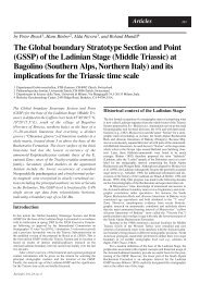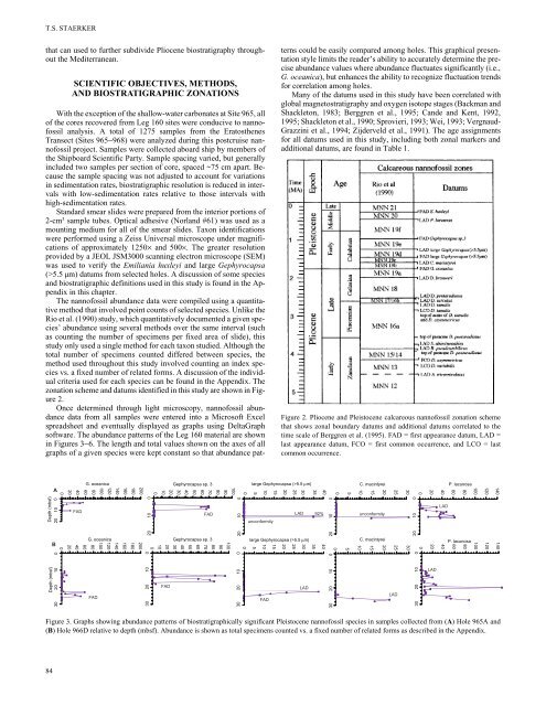Figure 2. Pliocene and Pleistocene calcareous nannofossil zonation scheme that shows zonal boundary datums and additional datums correlated to the time scale of Berggren et al. (1995). FAD = first appearance datum, LAD = last appearance datum, FCO = first common occurrence, and LCO = last common occurrence. A 0 10 20 30 40 50 60 70 80 90 100 0 30 25 20 15 10 5 35 40 0 5 0 20 40 G. oceanica 60 80 100 120 140 160 180 200 Gephyrocapsa sp. 3 large Gephyrocapsa (>5.5 µm) C. macintyrei P. lacunosa 30 25 20 15 10 80 60 40 20 0 100 120 140 Depth (mbsf) 20 10 0 FAD B 0 20 40 60 G. oceanica Gephyrocapsa sp. 3 large Gephyrocapsa (>5.5 µm) C. macintyrei P. lacunosa 80 100 120 140 160 180 200 0 10 20 30 40 50 60 70 80 90 100 5 0 30 25 20 15 10 80 60 40 20 0 100 120 140 0 0 10 FAD 0 10 unconformity LAD 92% 0 10 unconformity 0 10 LAD 20 20 20 20 40 35 30 25 20 15 10 5 0 0 Depth (mbsf) 30 20 10 0 0 0 FAD 10 20 30 FAD 10 20 30 FAD LAD 10 20 30 LAD 10 20 30 LAD Figure 3. Graphs showing abundance patterns of biostratigraphically significant Pleistocene nannofossil species in samples collected from (A) Hole 965A and (B) Hole 966D relative to depth (mbsf). Abundance is shown as total specimens counted vs. a fixed number of related forms as described in the Appendix. 84
CALCAREOUS NANNOFOSSIL BIOSTRATIGRAPHY BIOSTRATIGRAPHIC INTERPRETATIONS Hole 965A Only one hole was drilled at Site 965. The hole consisted of 27 cores that reached a total depth of 240.40 mbsf. Lithologies ranged from nannofossil ooze to clay in the upper four cores to packstones, grainstones, and wackestones containing only benthic foraminifers, mollusks, and algal laminations in Cores 160-965A-4H through 27X (Emeis, Robertson, Richter, et al., 1996). During postcruise nannofossil studies, 41 samples were analyzed from Core 160-965A-1H through 4H. Graphs showing species abundance patterns are shown in Figures 3 and 4. Emiliania huxleyi is present from Sample 160-965A-1H-1, 15−16 cm (0.15−0.16 mbsf) through 2H-1, 20−22 cm (1.00−1.02 mbsf), which indicates that these samples are in Zone MNN 21. The E. huxleyi acme (Zone MNN 21b) was not identified in Hole 965A. The scanning electron microscope (SEM) was used to verify the placement of the first appearance datum (FAD) E. huxleyi. In Sample 160-965A-2H-1, 109−110 cm (1.89−1.90 mbsf) through 2H-2, 105−106 cm (3.35−3.36 mbsf) Zone MNN 20 is recognized by the absence of both E. huxleyi and Pseudoemiliania lacunosa. The accompanying assemblage includes Rhadosphaera claviger, Gephyrocapsa oceanica, small gephyrocapsids, Calcidiscus leptoporus, Syracosphaera pulchra, and Scapholithus fossilis. Although it was not studied quantitatively, Helicosphaera kamptneri was observed to fluctuate significantly throughout these samples. Reworked Cretaceous, Eocene, and Pliocene species, in addition to clay-sized and silt-sized calcite particles, also fluctuated throughout these samples. Pseudoemiliania lacunosa becomes a consistent part of the assemblage beginning in Sample 160-965A-2H-3, 4−5 cm (3.84−3.85 mbsf). The presence of P. lacunosa means that this sample and those immediately below are within Zone MNN 19f. Although rare specimens of P. lacunosa were observed uphole, they were considered reworked. With the exception of an abundance peak in Sample 160- 965A-2H-3, 90−91 cm (4.70 mbsf), the uppermost 2.5 m of this zone is typified by low numbers of P. lacunosa (less than 2% P. lacunosa per 500 total coccolith count). Below 4.70 mbsf, P. lacunosa is a common part of the assemblage. The last appearance datum (LAD) of Gephyrocapsa sp. 3, which is reported by Rio et al., 1990 as an alternate marker within Zone MNN 19f, was observed in Sample 160-965A-2H-3, 90−91 cm (4.70−4.71 mbsf). The quantitative method for determining the presence (or absence) of Gephyrocapsa sp. 3 follows the criteria of Rio et al. (1990) and is described in the Appendix. The base of Zone MNN 19f, as indicated by the FAD of Gephyrocapsa sp. 3, is recognized in Sample 160-965A-2H-4, 116−117 cm (6.46−6.47 mbsf). An increase in abundance in P. lacunosa was also noticed at 6.46 mbsf. The recognition of the FAD and LAD of Gephyrocapsa sp. 3 in successive samples (1.08 m apart) suggests that either an unconformity exists between these samples or the samples are within an interval characterized by very low sedimentation rates (approximately 4.3 m/m.y.). The next significant change in the nannofossil assemblage occurs where large Gephyrocapsa (>5.5 µm) is recognized in Sample 160- 965A-2H-7, 28−29 cm (10.08−10.09 mbsf). Large Gephyrocapsa is observed in only two samples. The FAD was identified in Sample 160-965A-2H-CC (10.28−10.30 mbsf), whereas the LAD was identified in Sample 160-965A-2H-7, 28−29 cm (10.08−10.09 mbsf). Together, these two samples comprise Zone MNN 19d. In Sample 160-965A-3H-1, 21−22 cm (10.51−10.52 mbsf), Calcidiscus macintyrei becomes a common part of the nannofossil assemblage. Typically, the LAD of C. macintyrei signifies the top of Zone 19b; however, the absence of G. oceanica in this sample indicates that the sample is actually within Zone 19a. Collectively, the FADs of large Gephyrocapsa and G. oceanica (Sample 160-965A- 2H-CC) juxtaposed to the LAD of C. macintyrei (160-965A-3H-1, 21−22 cm) in successive samples indicates that an unconformity exists between 10.30 mbsf and 10.52 mbsf. Within the interval represented by the unconformity, sediments comprising Zones MNN 19c and MNN 19b are entirely missing, and portions of Zone MNN 19a and MNN 19d may also be missing. The missing sediments represent a length of time that ranges from a maximum of 1.10 Ma to 2.02 Ma, to a minimum span from 1.47 Ma to 1.72 Ma (Fig. 2 and Table 1). According to this interpretation, sediments spanning the Pleistocene/ Pliocene boundary are not present in Hole 965A. In Sample 160-965A-3H-1, 135−136 cm (11.65−11.66), a nannofossil assemblage typified by the presence of Discoaster brouweri and Discoaster triradiatus is observed. Owing to the absence of other discoasters, this sample is assigned to Pliocene Zone MNN 18. The accompanying assemblage includes C. leptoporus, C. macintyrei, small reticulofenestrids, and H. kamptneri. Discoaster pentaradiatus is observed in Sample 160-965A-3H-3, 99−100 cm (14.29−14.30 mbsf), which marks the uppermost limit of Zone 17−16b. At 15.72 mbsf, below the LAD of D. pentaradiatus, the LAD of Discoaster surculus is observed. Discoaster surculus is used in extra-mediterranean zonation schemes (Okada and Bukry, 1980; Martini,1971) as a zonal marker; however, in the Mediterranean, the LADs of D. pentaradiatus and D. surculus are virtually indistinguishable (Rio et al, 1990; Müller, 1978; Driever, 1981; and Ellis and Lohman, 1979). Following the zonation scheme of Rio et al. (1990), the two species are placed at the top of Zone MNN 17−16b. In Sample 160-965A-3H-5, 96−97 cm (17.26−17.27), Discoaster tamalis is observed in abundances greater than 2% of the total discoaster population. Following the criteria of Rio et al. (1990), the downhole increase in D. tamalis greater than 2% of the discoaster population indicates that this sample is within Zone MNN 16a. All occurrences of D. tamalis identified uphole were less than 2% and thus, are considered above the datum. Because D. tamalis fluctuates to rare or absent near its LAD, Rio et al. (1990) and Sprovieri (1993) cite the importance of using a close sample spacing to accurately identify the zonal boundary. The average sample spacing used in this study was 74 cm, which is considerably greater than the average spacings used by Rio et al. (1990) (40 cm to 10 cm) and Sprovieri (1993) (25 cm) in their respective studies. For this reason, the LAD of D. tamalis datum in this study may have been placed lower in the geologic record compared to the Rio et al. (1990) and Sprovieri (1993) studies. Discoaster tamalis remains a continual part of the nannofossil assemblage downhole and increases in abundance near 30% of the total discoaster assemblage in Sample 160-965A-4H-1, 42−43 cm (20.22−20.23 mbsf). The increase in abundance of D. tamalis is coincident with increases in the abundance of Discoaster asymmetricus and a single spike in the abundance pattern of D. pentaradiatus. In Sample 160-965A-4H-2, 29−30 cm (21.59−21.60 mbsf), immediately below the increases in D. tamalis and D. asymmetricus, Sphenolithus abies/neoabies becomes a consistent part of the assemblage. In addition to the LAD of Sphenolithus abies/neoabies, assemblage changes that include the absence of both D. pentaradiatus and D. tamalis, the dramatic decrease of D. asymmetricus, and a marked increase in the abundance of D. surculus are observed in Sample 160-965A-4H-2, 29−30 cm (21.59−21.60 mbsf). The absence of D. pentaradiatus in the lowermost portion of Zone MNN 16a is a consistent event observed in the Central Mediterranean and first described as a paracme event by Driever (1988). The assemblage that includes D. tamalis in the absence of R. pseudoumbilicus and D. pentaradiatus (paracme) is observed in only one sample in Hole 965A, which suggests that either the sedimentation rates are low or erosion has removed most of the D. pentaradiatus paracme interval in Hole 965A. Reticulofenestra pseudoumbilicus (Zone MNN 14−15) is present beginning in Sample 160-965A-4H-2, 97−98 cm (22.27−22.28 mbsf). In the following sample (23.15−23.16 mbsf), which is the deepest sample studied in Hole 965A, another significant change in 85
Page 1: Robertson, A.H.F., Emeis, K.-C., Ri
Page 5 and 6: CALCAREOUS NANNOFOSSIL BIOSTRATIGRA

7. quantitative calcareous nannofossil biostratigraphy of ... - Ispra

You also want an ePaper? Increase the reach of your titles

Delete template?

Save as template?