Equivalence Checking of Combinational Circuits using ... - CiteSeerX

Equivalence Checking of Combinational Circuits
using Boolean Expression Diagrams
Henrik Hulgaard, Poul Frederick Williams, and Henrik Reif Andersen
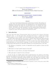
Abstract— The combinational logic-level equivalence problem is to determine
whether two given combinational circuits implement the same
Boolean function. This problem arises in a number of CAD applications,
for example when checking the correctness of incremental design changes
(performed either manually or by a design automation tool).
This paper introduces a data structure called Boolean Expression Diagrams
(BEDs) and two algorithms for transforming a BED into a Reduced
Ordered Binary Decision Diagram (OBDD). BEDs are capable of representing
any Boolean circuit in linear space and can exploit structural similarities
between the two circuits that are compared. These properties make
BEDs suitable for verifying the equivalence of combinational circuits. BEDs
can be seen as an intermediate representation between circuits (which are
compact) and OBDDs (which are canonical).
Based on a large number of combinational circuits, we demonstrate
that BEDs either outperform or achieve results comparable to both standard
OBDD approaches and the techniques specifically developed to exploit
structural similarities for efficiently solving the equivalence problem.
Due to the simplicity and generality of BEDs, it is to be expected that
combining them with other approaches to equivalence checking will be both
straightforward and beneficial.
Keywords— Tautology checking, combinational logic-level verification,
equivalence checking, Boolean circuits.
I. INTRODUCTION
HIS paper presents a technique for formally proving that
two combinational circuits implement the same Boolean
function. This verification problem, referred to as the combinational
logic-level equivalence problem, arises in a number of
CAD applications related to validating the correctness of a circuit
design:
¡ Due to the increase in the complexity of design automation
tools and the circuits they manipulate, such tools cannot in general
be assumed to be correct. Instead of attempting to formally
verify the design automation tools, a more practical approach is
to formally check that a circuit generated by a design automation
tool functionally corresponds to the original input (the specification).
Such a check is an instance of the combinational logiclevel
equivalence problem when the design automation tool only
manipulates the combinational portion of the circuit.
¡ The logic-level equivalence problem also arises when a circuit
is manually modified in order to accommodate special requirements
which cannot be handled by the design automation tool
(so-called engineering changes). The designer can ensure that
no functional errors have been introduced by verifying that the
original and modified designs are functionally identical.
¡ Finally, the combinational logic-level equivalence problem
arises as a sub-problem in other (higher-level) verification problems.
For example, when verifying arithmetic circuits by checking
that they satisfy a given recurrence equation [1] or when verifying
the equivalence of two state machines without performing
a state traversal [2].
Financially supported by the Danish Technical Research Council.
The authors are with the Department of Information Technology, Technical
University of Denmark. E-mails: {henrik,pfw,hra}@it.dtu.dk
The straightforward approach to solving the combinational
logic-level equivalence problem is to use Reduced Ordered Binary
Decision Diagrams [3] (OBDDs). To verify that two combinational
circuits with outputs ¢ and £ are equivalent, the
OBDD for ¤¦¥¨§ is constructed, where¤ and§ represent the
Boolean function for¢ and£ , respectively. Due to the canonicity
of OBDDs, the two circuits implement the same Boolean
function if and only if the resulting OBDD is identical to the
terminal © . This approach is simple and works well for many
circuits, but it has two inherent limitations:
¡ The first problem is that the size of the OBDD representation
for¤ and§ may be exponential in the size of the combinational
circuit, no matter what variable ordering is used. A well-known
example of this problem is the multiplication function which
Bryant [3] showed does not have any sub-exponential OBDD
representation for any variable ordering.
¡ The second problem is that OBDDs cannot exploit structural
similarities of the two circuits that are verified. Consider verifying
that two identical circuits implement the same Boolean
function. In this case, the full OBDD for both¤ and§ is constructed
before the identity of the circuits is verified. In typical
applications, the circuits to be verified are of course not identical,
but in all three application areas listed above, the two combinational
circuits are structurally similar. To efficiently verify
the circuits, it is essential to be able to exploit these similarities.
We suggest a newly developed data structure [4] called
Boolean Expression Diagrams (BEDs) for solving the combinational
logic-level equivalence problem. BEDs are an extension
of OBDDs that allow any Boolean circuit to be represented
in linear space. Furthermore, BEDs can recognize and share
identical sub-expressions. These properties eliminate the two
problems with the OBDD approach listed above and thus make
BEDs a promising data structure for solving the equivalence
problem.
The price one pays for the compactness of BEDs is that BEDs
are not canonical. Our approach to showing that the BED for
¤¥§ is a tautology is to transform it into an equivalent OBDD.
A key observation is that it is possible to construct the OBDD for
¤¥§ without constructing the OBDD for¤ and§ . For example,
the verification may succeed even if¤ and§ each represent a
multiplication function for which no small OBDD exists. Thus,
using BEDs, one can potentially avoid an exponential blowup
when computing the intermediate results.
The BED data structure is obtained by extending the OBDD
representation with operator vertices:
Definition 1 (Boolean Expression Diagram) A Boolean Expression
Diagram (BED) is a directed acyclic graph£
with vertex set and edge set . The vertex set contains
three types of vertices: terminal, variable, and operator vertices.
¡ A terminal vertex has as attribute a value !#"%$'&(*),+ .

Š
Š
Š
Š
Š
Ž
Š
Š
M
‡
A variable vertex has as attributes a variable -/.0' , and
¡
two 1 3245'667'8:9-7;'

Š
‘
Š
‘
—
Œ
Š
Š
— — ‹
‘
Š
‘
—
Œ
Š
‘
‹
‘
Š
—
Œ
Œ
Š
Œ
‘
‹
Œ
Œ
root 1
root 1
root 1
root 1
root 1
Œ3
Œ3
Œ3
Œ3
—
Š ‹
‹ ‹
root 1
ŒŽ Œ Œ
0 1
ŒŽ Œ Œ
0 1
ŒŽ Œ Œ
0
1
0
1
1
1
ŒŽ
(a) (b) (c)
(d)
(e)
(f)
Fig. 4. Steps used to show that root 1 from Fig. 3 is a tautology. a) to b) Use the identityỸmÚ#›œ˜0*žWŸ¦@š# o-ž . b) to c): Identify the two vertices. c) to d):
Identify the two› vertices. d) to e): Use the identity@šo¡wšNžEŸ€¢ . e) to f): Use the identity3£m¤¥ ¢/¦¢*žEŸ€¢ .
root 2
root 2
root 2
root 2
Œ@
Œ@
root 2
Œ3Ž
0
1
0
1
Œ@
0 1
1
1
(a)
(b) (c) (d) (e)
Fig. 5. Steps used to show that root 2 from Fig. 3 is a tautology. a) to b): Use the identityỸ3f›r@š

Š
Œ
Œ
Š
0
root 1 root 2
‘ ‘
Š
‹ Š
— —
Œm Œ3Ž Œ@
Fig. 3. The BED from Fig. 2 where variable£`¤ has been moved up.
1
problem. These techniques rely on the observation that if two
circuits are structurally similar, they will have a large number
of internal nodes that are functionally equivalent (typically, for
more than 80% of the nodes in one circuit, there exists a node in
the other circuit which is functionally equivalent [17]). This observation
is used in several ways. Brand [18] uses a test generator
for determining whether one node can be replaced by another
in a given context (the nodes need not necessarily be functionally
equivalent as long as the difference cannot be observed at
the primary output). If so, the replacement is carried out. In this
way, one circuit is gradually transformed into the other. The key
problem is to find a sufficiently large number of pairs, yet avoid
having to spend time testing all possible pairs of nodes. Several
heuristics are used to select candidate pairs of nodes to check,
e.g., the labeling of nodes and the results of simulation.
Test generation techniques are also the basis for the recursive
learning technique for finding logical implications between
nodes in the circuits by Kunz et al. [19], [20]. To enable the verification
of larger circuits, the recursive learning techniques can
be combined with OBDDs [21], [22]. The learning technique
is further extended by Jain et al. [23] and by Matsunaga [24],
introducing more general learning methods based on OBDDs
and better heuristics for finding cuts in the circuits to split the
verification problem into more manageable sizes.
Eijk and Janssen [25], [26] use the canonicity of OBDDs to
determine whether one node is functionally equivalent to another.
If two nodes are found to be identical, they are replaced
with a new free variable. Heuristics are used to select candidate
pairs of nodes to check for equivalence. The main problem with
this technique is to manage the OBDD sizes when eliminating
false negatives (when re-substituting OBDDs for the introduced
free variables).
Cerny and Mauras [27] present another technique for comparing
two circuits without representing their full functionality. A
relation that represents the possible combinations of logic values
at a given cut is propagated through the two circuits. A key
problem with this and the other cut-based techniques [21], [22],
[23], [24], [25], [26] is that the performance is very sensitive
to how the cuts are chosen and there is no generally applicable
method to choose appropriate cuts.
The technique by Kuehlmann and Krohm [17] represents the
most recent development of the structural methods, combining
several of the above techniques and developing better heuristics
for determining cuts. Kuehlmann and Krohm represent the combinational
circuits using a non-canonical data structure which is
similar to BEDs except that only conjunction and negation operators
are used. This data structure is only used to identify
isomorphic sub-circuits since no operator reductions are performed.
We believe that the structural technique by Kuehlmann
and Krohm would benefit significantly from replacing the used
circuit representation with BEDs since the continuous application
of the reduction rules would reduce the circuit representation
and help in identifying equivalent sub-circuits which in turn
would improve the performance of their technique.
BEDs can be seen as an intermediate representation between
the compact circuits and the canonical OBDDs. Compared to
the functional techniques, BEDs are capable of exploiting equivalences
of the two circuits and the performance is provably no
worse than when using OBDDs. Compared to the structural
techniques, BEDs only have a limited capability to find equivalences
between pairs of nodes (since only local operator reduction
rules are included). Combining BEDs with structural techniques
would be beneficial since information about equivalent
nodes immediately reduce the size of the BED and make even
further identifications of nodes possible.
During the last three decades the AI community has worked
on developing efficient satisfiability checkers. They could in
principle be used to solve the equivalence problem for combinational
circuits.
However, comparisons between algorithms
based on the prominent Davis-Putnam algorithm and OBDDs
show that although efficient for typical AI problems, they are
quite inferior to OBDDs on circuits [28].
Hachtel and Jacoby [29] describe an algorithm for solving
the equivalence problem by searching for a counterexample using
a tree formed by case splitting (co-factoring) the combined
circuits on the variables of the primary inputs. If during the generation
of the co-factor tree a subcircuit structurally equivalent
to a previously visited subcircuit is found, the previous result is
used. Equivalence is determined by matching the strings representing
the formula of the two subcircuits. On smaller circuits
(up to 100 gates) this approach is demonstrated to work well.
To some extent one of the algorithms of synthesizing OBDDs
from BEDs (UP_ONE) can be seen as an improved version of the
Hachtel-Jacoby algorithm in which the identification of equivalent
subcircuits is improved both by the use of reduction rules
and through the sharing of nodes.
The BED data structure is inspired by the MORE approach
[30], [31] to synthesizing OBDDs. MORE is based on
the observation that the OBDD for¤¨T§ can be constructed by
introducing a new variableJ and implicitly existentially quantifyJ
since©AJ(VJ~KL¤g§ª«¤¬T§ . MORE constructs the OBDD
by moving J towards the terminal vertices using the level exchange
operation [32]. The BEDs differ from the MORE ap-

proach by their use of operator reductions and the new synthesis
algorithms (which work on arbitrary BEDs where operators and
variables are freely mixed).
Prior to the work on MORE, Plessier et al. [33], [34] proposed
a variant of OBDDs called Extended BDDs (XBDDs) obtained
by adding structural variables which can be both universally and
existentially quantified. Quantifications are described as annotations
on pointers leading to nodes with structural variables.
The quantifications allow Boolean operations to be expressed.
During construction of an XBDD from a circuit, a trade-off can
be made between removing a structural variable and perform
OBDD synthesis or keeping the structural variable. Two algorithms
for checking satisfiability of XBDDs were given (one requiring
up to exponential space, the other requiring linear space
but exponential time). No algorithms for converting an XBDD
into a OBDD were given. Using the satisfiability algorithms the
authors showed that although the growth is still exponential, the
equivalence between the median bit of two structurally different
multiplier circuits could be proven for two 16 bit multipliers.
BEDs extend the ideas of XBDDs and MORE to include arbitrary
binary operators and allowing these operators to remain in
the graph while transforming it. (In XBDDs and in the MORE
approach, two nodes are needed to represent an exclusive-or or a
biimplication.) This makes it possible to include operator reduction
rules and develop new OBDD synthesis algorithms (e.g.,
UP_ONE) which are essential for obtaining the runtimes presented
in this paper.
B. Overview
The paper is organized as follows. The construction of BEDs
is presented in Section II. In Section III we described the algorithms
for transforming a BED into an equivalent OBDD. Section
IV describes two heuristics for choosing a variable ordering
based on the topology of the circuit. Section V presents the experimental
results, verifying a large number of combinational
circuits from the ISCAS 85 and LGSynth 91 benchmarks. Finally,
Section VI summarizes the contributions of this paper.
II. CONSTRUCTION OF BEDS
BED vertices are constructed using a single constant-time operation
called ­ªF®°¯b±g2*²N¯ . This operation ensures that the BED
is reduced and also performs several optimizations of the representation.
Contrary to OBDDs, reducedness will not make
BEDs canonical (not even when combined with a fixed variable
ordering.)
A. Reduced BEDs
We shall forbid the existence of redundant vertices, i.e., two
vertices representing isomorphic sub-BEDs and vertices that are
unnecessary for obvious reasons. For readability, we use³

‰
Ì
Î
Ô
Ô
Ô
Ì
Ô
X
‰
Š
‹
í:îB3ï†ð'¦Dñ0¦DòFž 1: is in tableóOô!õ*ö
reduction æxçè xùéGéúOëêké„êA¦ë°¦GìFžDž
2:
õ-û:ü õ´÷GõbóOø'÷6öœ`ïðA¦DñA¦DòFž
3:
1: í:îWþ is operatoróOô!õ-ö
2: ÷GõbóOø'÷6ö ý¡ ú 磢 é ènç æxçè `þg¦ ùm¦†ÿžxž
Š
Š
Since Boolean circuits can be transformed into a “DAG of OB-
DDs” in linear time (and space) and a (general) BED can be
transformed into a Boolean circuit in linear time (and space),
the last four classes are equally expressive. This is quite unlike
for OBDDs where there is an exponential gap between OBDDs
and free BDDs, and between free BDDs and BDDs.
ÎËß
’„Í
C. Operator reductions
For operator vertices one can add more checks in order to
reuse vertices, thereby reducing the size of the BED. An immediate
optimization is to ­ªF®°¯n±Y2F²°¯ extend to look for operator
vertices that differ from the one wanted only by exchanging
low and high, by a negation, or by a combination of both.
Going a step further, considering two vertices at a time, we
can eliminate all negations below binary operators since for
with
all binary 2O? operators there exists another 2O?
2? xpfbÁ'ÂÃ2?xÚ pfFÁ!
operator
. Finally, taking the identity of vertices
into account allows us to exploit equivalences like the absorption
e.g.,JT§DJRªÄ0«J laws, . arevFÅNÆ There combinations of
binary Boolean operators, thus it is feasible to tabulate them
Ç
forÇ
all up to three or
ChoosingÇ
«È
four.
allows us to determine operator 2-cuts. Consider
a BED with the structure shown in Fig. 6 (a), that is, for
vertexµ some , all fromµ paths to the terminals go through either
. set$FÉÊM/ ɡ+ The is a 2-cut and such a cut
vertexÉÊM orɡ
can be used to reduce the size of the BED as shown in Fig. 6 (b).
That is, all fromµ vertices to the operator 2-cut can be replaced
Î Þ
’„Ínà
X ß
ÎÝ
XÞ
’†Íbá
Fig. 7. A tree of three operator vertices.
Î Î Ž Î
â/ã
‹
Î Ž Î Î
Fig. 8. A reduction table foräŸ~å includes information on how each combination
of up to three BED operator vertices can be reduced. Here the reduction
rule for one of the distributive laws is used to eliminate one of the operator
vertices.
represented by fewer nodes. If this is possible, the reduction is
included in the reduction table. Thus, given three operator nodes
and the equivalences of the nodes and their children, it is possible
by a simple table lookup (performed in constant time) to
determine the optimal representation.
Fig. 9 shows the algorithms for constructing BED vertices
using the reduction rules. Vertices are created using ­5® which
calls the algorithm.GŌ² to apply the reduction rules. Notice how
the reduction rules are applied repeatedly until no more reductions
are possible.
X Ý
Only operator
vertices
æDç†è xé„êA¦ë!¦ ìFžkŸ
’†Í
õ-û:ü õ´÷GõbóOø'÷6ö ý¡ ú 磢 é ènç 3þg¦ ùm¦„ÿž
3:
Fig. TheæDç†è
andý
ú 9. algorithms.
(a)
(b)
Ì Ž
ý úN3þg¦Gùm¦†ÿžgŸ
Ì Ž
Fig. 6. A BED with an operator 2-cutÏGдÑ6¦xÐfÒ6Ó .
with a single operator vertex with³

¤
‰
‰
‰
‰
It is well known that not all 16 binary Boolean connectives
are needed to represent any Boolean expression. For example,
the sets {nand} and {or, not} are functionally complete. It is
therefore possible to limit the different operators in the BED to
those of any complete set. Choosing a small set, e.g., {nand},
the depth of the BED increases as several nand operators are
need to represent other operators like exclusive-or. To effectively
handle such cases, the reduction rules would need to look
to a greater depth to achieve equally powerful reductions. This,
however, greatly increases the number of cases to consider and
thus complicates the reduction-step. Keeping a depth of two
(i.e.,
Ç È ) with a minimal operator set like {nand}, overall
performance decreases since less reductions are performed. On
the other hand, using a small operator set has the advantage that
chances for identifying vertices increases since all operators are
expressed in terms of a small set of operators. We have found the
following set of operators to be a good trade-off between a small
and large operator set: {nand, or, right implication, left implication,
biimplication}. This set of operators has the property that
all ten non-trivial binary Boolean operators can be expressed
from it using exactly one operator or the negation of an operator
which can be absorbed by an operator immediately above it.
Thus, no more operator vertices are needed to represent a given
Boolean expression than using the full set of all 16 operators.
III. COMBINATIONAL VERIFICATION USING BEDS
The procedure VERIFY, shown in Fig. 10, determines whether
two combinational circuits implement the same Boolean function.
The input to VERIFY consists of the two combinational
In this section, we describe two algorithms for transforming
a BED into an equivalent OBDD. It should be observed that any
transformation algorithm from BEDs to OBDDs will necessarily
have exponential worst-case runtime (assuming º P NP). This
follows since determining SATISFIABILITY of a BED is NPcomplete
and determining TAUTOLOGY is co-NP-complete [36]
and these problems are easy for OBDDs.
It is easily seen that an (O)BDD is simply an (O)BED without
operators. This suggests a strategy for converting BEDs into
OBDDs: gradually eliminate the operators, keeping all the intermediate
BEDs functionally equivalent. We have developed
two very different ways of operator elimination called UP_ONE
and UP_ALL. In the following, it is assumed that the BEDs are
ordered (and thus also free). This assumption simplifies the algorithms
and does not limit the expressiveness of BEDs (see
Section II). It is straightforward to extend the algorithms to work
for the general class of (non-ordered, non-free) BEDs and these
algorithms have the same asymptotic runtime as the ones presented
here. The more general algorithms can be used, e.g., for
making a free BDD ordered (i.e., transforming it to an OBDD)
or for reordering an OBDD.
A. The Up-Step
A key operation on BEDs is the up-step which moves a variable
vertex up above an operator vertex. 2? Let be an arbitrary
binary Boolean letJ operator, be a Boolean variable, let¤ Œ and
(‚

‘
Œ3
‘
‹
Œ
Š
Š
Œ
Š
Š
‘
‹
Š
‹
Š
Š
‘
Œ
Š
Š
Š
‘
Š
—
Œ
‘
‹
‘
Œ
Š
Œ
—
‹
‘
‘
‹
—
Š
Œ3
Œ3
Œ3
Š Š Š
‹
Œ3
—
Œ
0
1
0
1
0
1
0
Œ@
1
(a)
(b) (c) (d)
ŒŽ
ŒŽ
Œ3Ž
Œ@
Œ3Ž
Œ3
Œ3
Œ3
Œ3
—
Œ
Œ
—
—
Œ
—
Œ
0 1
0 1
0 1
0 1
0 1
1
Œ3Ž
Œ@
Œ3Ž
Œ@
Œ@
Œ@
Œ@
(e)
(f) (g) (h) (i)
(j)
Fig. 12. Proving 6ïOï! DÒ that is a tautology. (a) The BED 6ïOï! DÒ for from Fig. (b)£`¤ 2. is moved above the three conjunctions (one being negated) using three
up-steps. Notice that, at this point, variable and operator vertices are no longer separated in two distinct layers. (c) Conjunctions with children that are constant
vertices are (d)£`¤ eliminated. is moved above the disjunction. (e) The disjunction with both children equal " to is (f)£m¤ removed. is moved above the negated
conjunction. (g) The conjunction with " a child is eliminated. The absorption ›W@šË œ*žBŸ à law
is applied. (h) The negation vertices are identified. (i)
Identifying the two vertices with£m¤ . At this point the two children of the biimplication operator are identical and (j) the BED is reduced to¢ , proving the
tautology.
exploit structural information in the expression (as was the case
in the example).
B. Construction of OBDDs with UP_ONE
The first elimination algorithm is based on the algorithm
UP_ONE shown in Fig. 13. UP_ONE pulls a single variable up
to the root by performing a recursive depth-first traversal of the
BED and after the recursive calls on the low- and high-child of a
vertex, it makes an up-step. Repeated calls to UP_ONE for each
variable moves all variables up past the operators, which makes
the operators disappear (by |‚†‚†‚„ requirement of reducedness).
The # table is used to memoize previously computed results
and ensures a linear expected runtime.
The example in Fig. 12 shows the steps of performing
ˆˆ
‡ . As the example illustrates, in fortunate
UP_ONE|‚„ƒ/$
cases a BED is converted into an OBDD after moving just a
few variables up (in the example, one variable was sufficient).
In this process, identical sub-BEDs, potentially containing operator
vertices, are identified. This is quite unlike traditional
OBDD construction where all operators are converted in depthfirst
order into OBDDs. In particular, an OBDD is constructed
for each sub-expression. If the result is small and the intermediate
OBDDs are large, UP_ONE is an attractive alternative.
The number of vertices in the BED reachable from a vertexµ
is denoted %µ&%0'%l$*(0µ)¨E+% . The following properties hold
for UP_ONE whenª UP_ONE|J(GµY :
¤YXœh¤ Î
.
|‚†‚*%+%, –-%µ.%-u v .
|‚
The running time of UP_ONE is /y!%µ.% .
D‚†‚‚
To use UP_ONE to transform a BEDµ into an OBDD with the
variable ordering J M ¿102030Ë¿ J Æ
, UP_ONE is called once for
each variable in the ordering:
Æ UP_ONEDJ Æ6 M FVbVbV UP_ONEDJ M µW+03020 WV
UP_ONEDJ
Even though UP_ONE has linear runtime and it is called only
54
Ç
times, the runtime of this computation is exponential in the
worst case due to the potential increase in size of the intermediate
results.

9
9
7 7 “ 8 7 “ 7:8
Î
9
9
Î
9
7 7 “
í:îB@š'¦Dñ!ž=@? óOô!õ-öo÷õnó6ø'÷OöA?¨CBN¦¨D/ž
1: õí]îYñ 2: is terminaló6ô!õ*öÊ÷GõbóOø'÷6ö#ñ
a õí]îWþg@ñ!ž 3: variablešióOô!õ-öË÷õnóOø'÷6öoñ
is
õ-û:ü õ 4:
FEm¦HGNžI¦ UP_ONE@š'¦ùéJxëžxž†¦ UP_ONE§K!¦ÿ2L MOÿ!xëžxžDž
5:
í]îWþg@ñ!ž 6: is a withì
6æ Dë/žONPKóOô!õ-ö
&¦ ý ú°xì 6æ Dë/ž†¦ùm¦„ÿž
7:
õ*û@üõí]îWþg§E@ž andþg§GNž 8: are variableš´ó6ô!õ*ö
both
&¦ ý ú°K!¦ ý úN3þgDë/ž†¦OùéJ´Dù@ž„¦ ùéJ|ÿžDž„¦
9:
õ*û@üõí]îWþg§E@ž 10: variableš´óOô!õ-ö
is
&¦ ý ú°K!¦ ý úN3þgDë/ž†¦OùéJ´Dù@ž„¦„ÿž„¦
11:
õ*û@üõí]îWþg§GNž 12: variableš´óOô!õ-ö
is
&¦ ý ú°K!¦ ý úN3þgDë/ž†¦Oùm¦ùéJ´|ÿžDž„¦
13:
14: õ*û@üõ
9
í:îBFE|¦SGNžT;>=U? ó6ô!õ*ö%÷GõbóOø'÷6öV?¨XẀ¦ZY/ž
APPLYé„ê0¦ùm¦ÿ2L MOÿ!|ÿžDžxž
1: í:îYñU;>=@RwóOô!õ*öÊ÷õnóOø'÷6öAR%3ñ°ž
UP_ALL@ñ!žkŸ
õí]îYñ 2: is terminaló6ô!õ*öÊ÷GõbóOø'÷6ö#ñ
a
õ-û:ü õ 3:
í]î[E 5: G and are verticesó6ô!õ*ö
terminal
&¦ ý úN3þgxëž„¦Oùm¦†ÿž
6:
õ*û@üõí]îYþg@ñ!ž 7: is variableš´óOô!õ-ö
a
&¦ ý úN§K'¦ ùm¦†ÿž
8:
õ*û@üõí]îfì 6æ xù@žkŸ%ì 6æ |ÿž!ó6ô!õ*ö
9:
&¦ ý úNDì 6æ Dù@ž„¦ UP_ALLý
10:
õ*û@üõí]îfì 6æ xù@ž+Nì 6æ |ÿž!ó6ô!õ*ö
11:
&¦ ý úNDì 6æ Dù@ž„¦ UP_ALLý
12:
õ*û@üõ=Qf¨`:_SaE3ñA¦Snž 15: R in
÷GõbóOø'÷6ö¡
16:
MOÿ!xù@ž†¦„ÿQL MOÿ!mÿ/žDžDžxž
APPLYxéêk¦ùm¦†ÿ/žÂŸ
’†Í
â/ã
’„Í
õí]î[EQ\]=Q^UYU\]_S`baS`£_Scd;>=e\]W>f°óOô!õ*ö
&¦
õ-û:ü
’†Í
7 “ 8 7£8
&¦
õ-û:ü õí]îBì 6æ xù@žkŸ%ì 6æ |ÿž!óOô!õ-ö
(a)
é„êkDì ùë ç Dù@ž„¦ ì ùë ç mÿžxž
ý ú°Dì 6æ Dù@ž†¦ APPLYé„ê0¦ùéJxù@ž†¦ ùéJ´|ÿžDž„¦
õí]îBì 6æ xù@ž+Nì 6æ |ÿž!óOô!õ-ö
&¦ ý ú°Dì 6æ Dù@ž†¦ APPLYé„ê0¦ùéJxù@ž†¦„ÿ/ž†¦
õ-û:ü
APPLYé„ê0¦†ÿ2L>Mÿ'Dù@ž„¦„ÿ2L>Mÿ'mÿžxžDž
&¦
õ-û:ü õMÿ'Dù@ž„¦„ÿžxž
7£8 7
7:8 7
(b)
7 8 7 Î
Fig. 11. Illustration of the up-step (a) for the case variableš where exists in
both children of the root and (b) for the whereš case only occurs in the left
child.
Fig. 14.
The APPLY-operation. Assumes E and G are OBDDs. The imposed
total order on the variable vertices is denoted N . In the code it is assumed
that terminal vertices are included at the end of this order when comparing
6æ xù@ž andì
6æ mÿž . The memoization table R must be initialized to empty
prior to the first call.
ì
ý ú°Dì 6æ mÿž„¦ APPLYé„ê0¦ùm¦GùéJ´|ÿžDž„¦
â/ã
â/ã
;>=f¨`:_SaExXẀ¦SY/ž„¦S_„ž=i?
X ’„Í ’„Í
÷õbóOø'÷6öË÷
UP_ONE3š'¦xñ°žEŸ
FEm¦¨GNž-¦ UP_ALLDùéJ´Dë/žDž„¦ UP_ALL|ÿ2L MOÿ!xëžxžDž
4:
and G are OBDDs j /
/jOE
úN3þgxëž„¦OùéJ´xù@ž†¦GùéJ´|ÿžDžxž†¦
UP_ALLý
úN3þgxëž„¦Gÿ2L
ý úN3þgDë/ž†¦Gÿ2L>Mÿ'Dù@ž„¦„ÿ2L>Mÿ'mÿžxžDž
UP_ALLý
úN3þgxëž„¦Gÿ2L MOÿ!xù@ž†¦„ÿ/žDžDž úN3þgxëž„¦OùéJ´xù@ž†¦ÿžDž„¦
ý úN3þgDë/ž†¦Gÿ2L>Mÿ'Dù@ž„¦„ÿžxž
UP_ALLý
úN3þgxëž„¦Oùm¦†ÿ2L MOÿ!|ÿžDžxžDž úN3þgxëž„¦Oùm¦ùélJ´mÿžxžDž†¦
&¦ ý ú°`þgDë/ž†¦ùm¦†ÿž
15:
insertx@š'¦ñ°ž†¦¨6ž 16: R in
÷GõbóOø'÷6ö¡
17:
Fig. 13. The UP_ONE-operation. UP_ONE takes an BEDñ ordered as argument
and returns an equivalent withš BED pulled up as far as possible without
violating the ordering. The imposed total order on the variable vertices is
N denoted . The memoization R table must be initialized to empty prior to
the first call.
C. Construction of OBDDs with UP_ALL
An alternative way to construct an OBDD is to move all variables
up simultaneously, called UP_ALL. UP_ALL is a generalization
of Bryant’s APPLY-operator, shown in Fig. 14. Construction
of OBDDs from a Boolean expression using recursive
calls of APPLY suggests a bottom up conversion of BEDs into
OBDDs. The UP_ALL algorithm does that by moving all variables
up as a block past the operator vertices. UP_ALL is shown
in Fig. 15.
Letµ be a vertex in a BED and let ¦ UP_ALL|µW . Then
Fig. 15. The UP_ALL-operation on OBEDs. The total N order is defined as
for APPLY (see Fig. 14). The memoization R table must be initialized to
empty prior to the first call.
UP_ALL has the following key properties:
¤YX«¤ Î
.
D‚†‚„ is an OBDD.
|‚
If z and } are OBDDs, then APPLYG2O?;F„O7E
|‚†‚†‚„
­y*®N¯b±g2*²N¯'2?b„67kG .
D‚†' If z and } are OBDDs, the running time of
UP_ALL
is /y$%z$%F%}m% .
UP_ALL2?´b„67k
D‚‚†‚ Properties D‚A and make clear the relation between
UP_ALL and APPLY. The time to build an OBDD bottom up using
APPLY (the standard way) and building it from a BED using
UP_ALL is within a constant factor. Experiments have shown
that the time to construct an OBDD using UP_ALL is comparable
to that of state-of-the-art OBDD packages and due to the
operator reductions, it can be significantly faster. However, the
worst-case runtime of UP_ALL is exponential %µ.% in , but for the
same reason as UP_ONE, this is optimal.
ý úN3þgDë/ž†¦Oùm¦†ÿQL MOÿ!mÿ/žDžDž

IV. VARIABLE ORDERING
The efficiency of UP_ONE and UP_ALL depends on the variable
order. Although the initial and final size of the BEDs are
independent on the variable order when the two circuits implement
the same function and thus the result is tautology© the , the
size of the intermediate BEDs depend on the ordering.
A large number of variable ordering heuristics have been developed
for OBDDs based on the topology of a circuit [33], [38],
[39], [40], [41], [42], [43]. The heuristics attempt to statically
determine a variable order such that the OBDD representation
of the circuit is small. Typically, these heuristics consist of two
steps to obtain a single global variable order: first, an order of
the primary outputs is constructed, then for each of the primary
outputs in this order, the variables in the support of the output
are ordered. We only consider the second step (finding a variable
order for a given primary output), since different variable orders
can be used for different roots of a BED (see Fig. 10). This allows
a greater flexibility to find good variable orders since the
orders of the primary outputs are independent. However, the
cost is that there is only limited reuse between verifying different
primary outputs.
Since UP_ALL essentially works as an improved APPLY
|‚†‚†‚ (property ), the variable orders that are good for OBDDs
will also be good orders to use with UP_ALL. Thus, when using
UP_ALL we can immediately use the variable ordering heuristics
developed for OBDDs.
Since UP_ONE works quite differently than UP_ALL, the variable
ordering heuristics developed for OBDDs may not be effective
when using UP_ONE. However, our experiments show
that this is not so; a good OBDD variable order also keeps
the intermediate BEDs small when constructing an OBDD with
UP_ONE. The reason for this is that a good variable order for
OBDDs has dependent variables close in the order. This allows
UP_ONE to collapse sub-circuits early in the verification process.
Also, a good variable order has the variables that affect the
output the most early in the order. UP_ONE will then pull these
variables to the root first which allows the most reductions. An
example of this was the of‚ ƒ use in the introductory example in
Fig. 3.
In the following we present two variable ordering heuristics,
originally developed for OBDDs, which have proven to be effective
for BEDs.
A number of variable ordering heuristics are based on a depthfirst
traversal of the circuit [39], [41], [42]. A depth-first traversal
is a simple and fast heuristic that has shown to be practical
for most combinational circuits [33], [39] since inputs that are
close together in the circuit are also placed together in the ordering.
The depth-first based heuristics differ in how they decide in
what order the inputs of a gate are visited. The FANIN heuristic
by Malik et al. [42] uses the depth of the inputs to a gate to
determine in what order to consider the inputs. The depth of a
terminal or variable is” vertex and the depth of an operator
texµ
ver-
n5oepWG²N¯„?q|7B3245·g 6-²N¯„?q|7B7A8:9*7B ·E GUrq) is . The total
runtime of FANIN to determine the variable order s of roots is
Ç [42] whereÇ
is the total number of reachable vertices
/yts
from s the roots.
The FANIN heuristic does not capture that variables affecting
the output the most should be ordered first, something which
is particularly important for UP_ONE. The DEPTH_FANOUT
heuristic [43] attempts to determine the variables that affect an
output the most by propagating a value from the output backwards
towards the primary inputs. The value is distributed
evenly among the input signals to a gate: if a value of u is assigned
to the output of a gate withÇ
input signals, the value assigned
to each of theÇ
fanin signals is incremented by u2v Ç
(the
signal may be input to several gates and thus obtains a contribution
from each gate). After propagating the value throughout
the circuit to the primary inputs, the DEPTH_FANOUT heuristic
adds the primary input with the highest value to the variable order.
This input is then removed from the circuit and the process
is repeated until all variables in the support have been included
in the variable order. The runtime of DEPTH_FANOUTDµY is
s the andt roots is the number of variables (inputs to the circuit).
Thus, this heuristic takes slightly longer to compute than
FANIN.
/yxtws Ç whereÇ
is the total number of reachable vertices from
V. EXPERIMENTAL RESULTS
In this section, we report the results from verifying a number
of multi-level combinational circuits from the ISCAS 85 and
LGSynth 91 benchmarks 2 .
The ISCAS 85 benchmark consists of eleven multi-level combinational
circuits, nine of which exist both in a redundant and
a non-redundant version. Furthermore, the benchmark contains
five circuits that originally were believed to be non-redundant
versions but it turned out that they contained errors and weren’t
functionally equivalent to the original circuits [20].
The circuits in the ISCAS 85 benchmark are by some researchers
considered too simple to use as benchmark circuits
with todays technology. This may be true for some application
areas but these circuits have several properties that make them
suitable as benchmark circuits for evaluating techniques for performing
a combinational logic-level verification. First, the circuits,
although quite small, are not easy to verify both due to
their functionality (for example, one of the circuits is a multiplier
for which OBDD techniques fail) and due to a rather large
logic-depth (up to 125 logic levels). Even with recent structural
techniques, some of these circuits take more than an hour to verify
[21]. Secondly, the circuits in the ISCAS 85 benchmark are
ideally suited for testing logic-level verification techniques since
they come in two functionally equivalent versions.
To evaluate the BED technique on a broader and more realistic
class of circuits, we also consider the 77 multi-level
combinational circuits and the 40 sequential circuits from the
LGSynth 91 benchmark. These circuits do not come in two versions,
so instead we map each of the circuits to a gate library
using SIS [7] and then optimize the circuits with respect to area.
We then verify that 1) the mapped circuit corresponds to the
original description, and 2) that the mapped and the optimized
circuits implement the same functionality. Due to the nature of
the mapping and optimization steps, the circuits differ in structure
considerably more than the ISCAS 85 circuits.
All experiments are carried out on a 300 MHz Pentium II PC
running Linux. Verification approaches based on decision dia-
These benchmarks are available from The Collaborative Benchmarking Laboratory
(http://www.cbl.ncsu.edu/)
Ò

grams typically run out of memory before running out of time.
Thus, to demonstrate the effectiveness of BEDs, in all experiments
we limit the memory consumption to 32 MB divided between
28 MB of memory to the node table (that is 1.46 million
nodes corresponding to 20 bytes per node) and 4 MB to caches.
The runtimes to determine the variable orders are insignificant
(at most two seconds for any of the circuits) when using the
FANIN heuristic. Using the DEPTH_FANOUT heuristic it takes
less then three seconds for the ISCAS 85 circuits, less than five
seconds for the combinational LGSynth 91 circuits, and less
than ten seconds for the sequential LGSynth 91 circuits except
for the circuits s15850.1, s38417, and s38584.1 which
take 33.7, 111.8, and 94.1 seconds, respectively. The times to
determine variable orders are not included in the CPU times reported
in the following, making a direct comparison between the
different verification approaches possible.
A. The ISCAS 85 circuits
Table I shows the size of the ISCAS 85 circuits and Table
II shows the runtimes to perform the equivalence check using
BEDs. When using UP_ONE, the DEPTH_FANOUT heuristic
TABLE I
SIZE OF THE ISCAS 85 BENCHMARK CIRCUITS.
Circuit Inputs Outputs Gates
c432/nr 36 7 433
c499/nr 41 32 516
c499/c1355 41 32 868
c1355/nr 41 32 1204
c1908/nr 33 25 2134
c2670/nr 157 63 2603
c3540/nr 50 22 3901
c5315/nr 178 123 6018
c6288/nr 32 32 4847
c7552/nr 207 107 8067
TABLE II
RUNTIMES (IN CPU SECONDS) FOR VERIFYING EQUIVALENCE OF THE
REDUNDANT AND NON-REDUNDANT CIRCUITS IN THE ISCAS 85
BENCHMARK. FOR EACH PAIR OF CIRCUITS, THE TIME IS GIVEN WHEN
USING THE TWO DIFFERENT VARIABLE ORDERING HEURISTICS FANIN AND
DEPTH_FANOUT (ABBREVIATED D._F.) AND USING THE TWO DIFFERENT
ALGORITHMS FOR TRANSFORMING A BED INTO AN OBDD, UP_ONE AND
UP_ALL. THE BEST RUNTIMES ARE HIGHLIGHTED USING BOLDFACE. A
’ REPRESENTS THAT THE VERIFICATION FAILED DUE TO LACK OF
‘x
MEMORY.
UP_ONE UP_ALL
Circuit FANIN D._F. FANIN D._F.
x x x
c432/nr 2.5 2.2 2.1 2.2
c499/nr 5.2 2.6 2.4 2.6
c499/c1355 1.6 1.6 1.6 1.6
c1355/nr 5.3 2.6 2.6 2.6
c1908/nr 1.0 1.0 1.0 1.0
c2670/nr 1.4 1.2 1.0 1.0
c3540/nr 16.9 21.8 17.0 33.7
c5315/nr 17.8 3.1 3.1 3.1
c7552/nr 4.6 3.7 2.6 2.6
c6288/nr 2.0
generally computes a better variable order than FANIN, while
there is little difference between the two ordering heuristics
when using UP_ALL.
The performance of UP_ONE and UP_ALL is comparable except
for the circuit c6288 where only UP_ONE succeeds. This
circuit implements a 16-bit multiplier for which it is known that
the OBDD representation grows exponentially [3]. The OBDD
representation of a 16-bit multiplier uses more than 40 million
vertices [44] and this number is approximately 2.7 times larger
for each additional bit in the operands. Thus, UP_ALL will fail
on this circuit no matter what variable ordering is used. In contrast,
UP_ONE never builds the OBDD representation of the multiplication
function and thus the circuits can be verified in just a
few seconds.
A.1 Proving Non-Equivalence
Table III shows the runtimes to determine non-equivalence
of the erroneous ISCAS 85 circuits. The reported CPU times
are for finding all errors. Although it does take longer to prove
non-equivalence, as expected since less equivalences exist, the
increase in the runtimes is insignificant.
TABLE III
RUNTIMES (IN CPU SECONDS) FOR SHOWING NON-EQUIVALENCE OF THE
REDUNDANT AND NON-REDUNDANT CIRCUITS IN THE ISCAS 85
BENCHMARK.
UP_ONE UP_ALL
Circuit # errs. FANIN D._F. FANIN D._F.
x x
c1908/nr_old 1 1.0 1.0 1.0 1.0
c3540/nr_old 5 26.6 23.3 17.3 27.9
c5315/nr_old 33 29.1 4.3 3.6 3.5
c2670/nr_old 6 6.5 1.3
c7552/nr_old 28 7.0 8.7 2.9 3.6
A.2 Effect of Operator Reductions
To illustrate the effect of operator reductions, we repeat the
experiments in Table II and III but without performing any of
the operator reductions described in Section II-C. The only reductions
performed are those required to maintain reducedness,
see Definition 1. The operation of UP_ALL then reduces to that
of APPLY, that is, the performance of UP_ALL corresponds very
closely to that of APPLY in a reasonable implementation of an
OBDD package. The results are shown in Table IV. Clearly, the
efficiency of UP_ONE relies heavily on the operator reductions
to identify identical nodes in the BED and thus avoiding to transforming
them into OBDDs. Without reductions, a large number
of the circuits cannot be verified (with 32 MB of memory) and
the runtimes for those that do succeed are up to several orders
of magnitude longer.
When using UP_ALL the situation is quite different. In building
an OBDD using UP_ALL, any vertex that is constructed during
the transformation will have non-operator vertices as the
children. I.e., whenever­y*®N¯b±g2*²N¯'x³iF„O7E is called in the body
of UP_ALL, bothz and} are variable or terminal vertices. Thus,
the operator reductions only affect the performance of UP_ALL
by reducing the initial size of the BED. For some circuits (e.g.,
c3540) this initial reduction has a large impact on the runtime

TABLE IV
RUNTIMES (IN CPU SECONDS) FOR VERIFYING EQUIVALENCE OF THE
y
REDUNDANT AND NON-REDUNDANT CIRCUITS IN THE ISCAS 85
BENCHMARK WITHOUT PERFORMING OPERATOR REDUCTIONS.
UP_ONE UP_ALL
Circuit FANIN D._F. FANIN D._F.
x
x
x
x
x
x
x
x x x x
c432/nr 2.9 2.6 2.5 2.3
c499/nr 166.1 2.5 4.1
c499/c1355 532.5 3.9 4.8
c1355/nr 743.5 4.1 4.8
c1908/nr 15.3 1.0 1.0
c2670/nr 29.0 1.4 1.9
c3540/nr 111.7 56.9 145.4
c5315/nr 4.8 3.5 3.3
c7552/nr 7.4 7.2 3.1 3.7
c6288/nr
c3540/nr_old 116.4 60.4 126.4
c5315/nr_old 6.0 4.0 3.7
c2670/nr_old 1.5
c7552/nr_old 10.0 15.2 3.1 4.1
of UP_ALL. This experiment indicates that performing an initial
operator reduction step, as discussed in the introduction, can
improve the time to construct an OBDD.
B. The LGSynth 91 Benchmarks
By construction, the redundant and non-redundant versions
of the ISCAS 85 benchmark circuits have many structural similarities
and are thus ideally suited for the BED approach.
To test the verification strategy on a broader range of circuits
with fewer structural similarities, we consider the circuits
from the LGSynth 91 benchmark. This benchmark includes
77 multi-level combinational circuits and 40 sequential
circuits. These circuits are mapped to a gate library
(msu.genlib) using SIS and then optimized for area using the
SIS script script.algebraic. As mentioned above, there
are two verification problems: one is to verify that the original
circuits correspond to the mapped versions and one is to verify
the mapped versions against the optimized versions. Due to the
nature of the mapping and optimization steps, the circuits differ
in structure considerably more than the ISCAS 85 circuits. The
results for the 77 combinational circuits are shown graphically
in Fig. 16. The eleven ISCAS 85 circuits are included in the
LGSynth 91 benchmark and although some of the LGSynth 91
circuits are considerably larger than the ISCAS 85 circuits, the
ISCAS circuits are the most difficult ones to verify using the
BED approach. The mapping of each circuit is verified in less
than three minutes. The results for the verification of the optimization
step are similar, except that the verification of the optimization
step of C6288 failed using both UP_ONE and UP_ALL.
The results for the verification of (the combinational portion
of) the 40 sequential circuits in the LGSynth 91 benchmark are
shown in Fig. 17. The mapping of the traditionally difficult circuit
s38417 takes 20 minutes to verify and the verification of
mm9b fails for both variable ordering heuristics. The mapping of
the remaining 38 circuits is verified in less than one minute. The
optimization of each circuit, except for mm9b and s38417, is
also verified in less than one minute. The verification of mm9b
and s38417 both fail when using 32 MB of memory. Using
64 MB of memory, s38417 is verified in an hour using the
FANIN ordering heuristic. The circuit mm9b is an instance where
the two ordering heuristics fail to construct a good variable order,
thus the verification of both the mapping and the optimization
steps fail, even when using 64 MB of memory. Using the
order in which the variables appear in the specification, the mapping
of mm9b is verified using 64 MB of memory in 207 seconds
and 270 seconds using UP_ONE and UP_ALL, respectively. Similarly,
the optimization of mm9b is verified in 69 seconds and
115 seconds using UP_ONE and UP_ALL, respectively.
C. Comparisons of Results
The ISCAS 85 benchmark has been used extensively by researchers
to test techniques for solving the equivalence problem.
Since all researchers have solved the exact same verification
problems, there is a good basis for comparing the different
approaches. Table V shows the runtimes to verify the ISCAS 85
circuits using recent methods.
The experiments are carried out on different machines and are
therefore not directly comparable. However, the efficiency of
the machines only differ by a small constant and not by orders of
magnitude and therefore the comparisons still give a good indication
of the relative virtues of the different approaches. The experiments
of Brand [18] is an exception since he does not report
runtimes for comparing the redundant and the non-redundant
versions. Instead the circuits are synthesized and optimized,
much in the same way as we have done for the LGSynth 91 circuits.
This might well be a more difficult verification problem.
From Table V it is clear that the learning-based approaches [21],
TABLE V
RUNTIMES (IN CPU SECONDS) OF OTHER APPROACHES FOR VERIFYING
THE ISCAS 85 BENCHMARKS. NOTICE THAT THE RESULTS OF
BRAND [18] ARE NOT DIRECTLY COMPARABLE SINCE A DIFFERENT
VERIFICATION PROBLEM IS SOLVED. “N/A” DENOTES THAT THE RUNTIME
HAS NOT BEEN REPORTED.
Circuit BED [18] [21] [22] [24] [26] [45]
c432/nr 2.1 4.0 1.0 2.0 0.8 0.2 0.4
c499/nr 2.4 38.0 1.9 5.0 1.2 0.2 0.4
c1355/nr 2.5 9.0 6.6 20.0 3.4 0.5 1.0
c1908/nr 1.0 22.0 11.2 22.0 6.2 1.6 2.1
c2670/nr 1.0 58.0 159.3 61.0 3.9 0.8 3.4
c3540/nr 16.9 39.0 67.6 281.0 17.4 3.0 12.7
c5315/nr 3.1 29.0 372.8 190.0 14.0 2.7 8.3
c6288/nr 2.0 193.0 21.5 40.0 9.1 4.3 7.2
c7552/nr 2.6 136.0 5583.3 412.0 20.6 34.6 20.8
c1908/old 1.0 n/a n/a n/a n/a 2.5 n/a
c2670/old 1.3 n/a n/a n/a n/a 54.6 n/a
c3540/old 17.3 n/a n/a n/a n/a 2.9 n/a
c5315/old 3.5 n/a n/a n/a n/a 8.3 n/a
c7552/old 2.9 n/a n/a n/a n/a 26.2 n/a
[22] are inefficient for larger circuits. The runtimes of the BED
approach is generally comparable to (and sometimes better than)
the other three approaches [24], [26], [45]. Moreover, these runtimes
should be seen in the light of the fact that the BED experiments
only use 32 MB of memory.
Only van Eijk [26] has reported runtimes for the erroneous
ISCAS 85 circuits. For these circuits it is observed that the BED

Fig. 16.
Ë
Ê Ç
Æ
ÉÈÄÇ
 Ã
Ä
ÅÂ Æ
¾¿
ÀÁ
¤2£

PC using only 32 MB of memory. Even known difficult circuits
(like s38417) are verified using modest resources (in less than
an hour with 64 MB of memory). This demonstrates that BEDs
combined with very simple algorithms are effective for solving
the combinational logic-level equivalence problem.
BEDs can be seen as an intermediate form between the compact
circuits and the canonical OBDDs, and thus combines the
functional and the structural verification techniques. All standard
OBDD operations can be performed on BEDs as well.
Some operations, like existential quantification and substitution,
can be performed directly on the data structure by using
UP_ONE [4], making the runtime of these operations linear in
the size of the BED. Other operations, like satisfiability and
tautology, can be performed by transforming the BED into an
equivalent OBDD.
Due to the simplicity and generality of BEDs, it is to be expected
that combining them with other approaches to equivalence
checking will be both straightforward and beneficial. The
benefits could be in two directions. Firstly, BEDs could be used
either as a “filter” in the filter-based approaches [45] or as the
basic data structure for representing circuits in any of the other
approaches allowing, for instance, a gradual and smooth transition
from circuits to BDDs. Secondly, BEDs could benefit from
other equivalence checkers. Whenever two subcircuits by some
means can be determined equivalent, the corresponding nodes
of the BED could be merged into one, resulting in an immediate
reduction in size. Moreover, this immediate reduction could
result in further reductions being possible by the reduction rules
and improve on the efficiency on later BDD-conversions.
BEDs are particularly useful in applications where the endresult
as an OBDD is small, for example, for tautology checking.
Another area that may benefit from using the BED representation
is symbolic model checking. Several researchers
have observed that when performing fixed-point iterations using
OBDDs, the intermediate results are often much larger than
the final result. Clearly, the succinctness of BEDs compared to
OBDDs can alleviate this problem. In fact, many of the tricks
researchers have used to make OBDDs more efficient are embodied
in BEDs. For example, Burch, Clarke, and Long [46]
demonstrated that the complexity of BDD-based symbolic verification
is drastically reduced by using a partitioned transition
relation where the transition relation is represented as an implicit
conjunction of OBDDs. This corresponds to representing
the transition relation as a BED with conjunction vertices at the
top level and only lifting the variables up to just under these
vertices.
REFERENCES
[1] M. Fujita, “Verification of arithmetic circuits by comparing two similar
circuits,” in Computer Aided Verification (CAV). 1996, Lecture Notes in
Computer Science, pp. 159–168, Springer-Verlag.
[2] C.A.J. van Eijk, “Sequential equivalence checking without state space
traversal,” in Proc. International Conf. on Design Automation and Test of
Electronic-based Systems (DATE), 1998.
[3] R. E. Bryant, “Graph-based algorithms for Boolean function manipulation,”
IEEE Transactions on Computers, vol. 35, no. 8, pp. 677–691, Aug.
1986.
[4] H. R. Andersen and H. Hulgaard, “Boolean Expression Diagrams,” in
IEEE Symposium on Logic in Computer Science (LICS), July 1997.
[5] R. B. Boppana and M. Sipser, “The complexity of finite functions,” in
Handbook of Theoretical Computer Science, J. van Leeuwen, Ed., vol.
A: Algorithms and Complexity, pp. 758–804. Elsevier Science Publisher,
1990.
[6] T. H. Cormen, C. E. Leiserson, and R. L. Rivest, Introduction to Algorithms,
MIT Press, 1990.
[7] E. Sentovich et al., “SIS: A system for sequential circuit synthesis,” Tech.
Rep. Memorandum No. UCB/ERL M92/41, Electronics Research Laboratory,
Dept. of EECS, University of California, Berkeley, 1992.
[8] R. Drechsler, A. Sarabi, M. Theobald, B. Becker, and M.A. Perkowski,
“Efficient representation and manipulation of switching functions based
on ordered Kronecker functional decision diagrams,” in Proc. ACM/IEEE
Design Automation Conference (DAC), 1994, pp. 415–419.
[9] U. Kebschull, E. Schubert, and W. Rosenstiel, “Multilevel logic synthesis
based on functional decision diagrams,” in Proc. European Conference on
Design Automation (EDAC), 1992, pp. 43–47.
[10] J. Gergov and C. Meinel, “Efficient Boolean manipulation with OBDD’s
can be extended to FBDD’s,” IEEE Transactions on Computers, vol. 43,
no. 10, pp. 1197–1209, Oct. 1994.
[11] E. I. Goldberg, Y. Kukimoto, and R. K. Brayton, “Canonical TBDD’s
and their application to combinational verification,” in Proc. International
Workshop on Logic Synthesis, 1997.
[12] J. Jain, J. Bitner, M. S. Abadir, and J. A. Abraham amd D. S. Fussell, “Indexed
BDDs: Algorithmic advances in techniques to represent and verify
Boolean functions,” IEEE Transactions on Computers, vol. 46, no. 11, pp.
1230–1245, Nov. 1997.
[13] D. Sieling and I. Wegener, “Graph driven BDDs – a new data structure for
Boolean functions,” Theoretical Computer Science, vol. 141, no. 1-2, pp.
283–310, 1995.
[14] R. I. Bahar, E. A. Frohm, C. M. Gaona, G. D. Hachtel, E. Macii, A. Pardo,
and F. Somenzi, “Algebraic decision diagrams and their applications,”
in Proc. International Conf. Computer-Aided Design (ICCAD), 1993, pp.
188–191.
[15] R. E. Bryant and Y.-A. Chen, “Verification of arithmetic functions with
binary moment diagrams,” in Proc. ACM/IEEE Design Automation Conference
(DAC), 1995, pp. 535–541.
[16] E. M. Clarke, K.L. McMillan, X. Zhao, M. Fujita, and J. Yang, “Spectral
transforms for large Boolean functions with application to technology
mapping,” in Proc. ACM/IEEE Design Automation Conference (DAC),
1993, pp. 54–60.
[17] A. Kuehlmann and F. Krohm, “Equivalence checking using cuts and
heaps,” in Proc. ACM/IEEE Design Automation Conference (DAC), 1997,
vol. 34, pp. 263–268.
[18] D. Brand, “Verification of large synthesized designs,” in Proc. International
Conf. Computer-Aided Design (ICCAD), 1993, pp. 534–537.
[19] W. Kunz, “HANNIBAL: An efficient tool for logic verification based on
recursive learning,” in Proc. International Conf. Computer-Aided Design
(ICCAD), 1993, pp. 538–543.
[20] W. Kunz and D. K. Pradhan, “Recursive learning: A new implication
technique for efficient solutions to CAD problems – test, verification, and
optimization,” IEEE Transactions on Computer Aided Design, vol. 13, no.
9, pp. 1143–1158, Sept. 1994.
[21] W. Kunz, D. K. Pradhan, and S. M. Reddy, “A novel framework for logic
verification in a synthesis environment,” IEEE Transactions on Computer
Aided Design, vol. 15, no. 1, pp. 20–32, Jan. 1996.
[22] D. K. Pradhan, D. Paul, and M. Chatterjee, “VERILAT: Verification using
logic augmentation and transformations,” in Proc. International Conf.
Computer-Aided Design (ICCAD), Nov. 1996.
[23] J. Jain, R. Mukherjee, and M. Fujita, “Advanced verification techniques
based on learning,” in Proc. ACM/IEEE Design Automation Conference
(DAC), 1995, pp. 629–634.
[24] Y. Matsunaga, “An efficient equivalence checker for combinational circuits,”
in Proc. ACM/IEEE Design Automation Conference (DAC), 1996,
pp. 629–634.
[25] C.A.J. van Eijk and G. L. J. M. Janssen, “Exploiting structural similarities
in a BDD-based verification method,” in Theorem Provers in Circuit
Design. 1994, number 901 in Lecture Notes in Computer Science, pp.
110–125, Springer-Verlag.
[26] C.A.J. van Eijk, Formal Methods for the Verification of Digital Circuits,
Ph.D. thesis, Technische Universitet Eindhoven, 1997.
[27] E. Cerny and C. Mauras, “Tautology checking using cross-controllability
and cross-observability relations,” in Proc. International Conf. Computer-
Aided Design (ICCAD), 1990.
[28] T. E. Uribe and M. E. Stickel, “Ordered binary decision diagrams and the
Davis-Putnam procedure,” in 1st International Conference on Constraints
in Computational Logics, J.P. Jouannaud, Ed., Sept. 1994, vol. 845 of Lecture
Notes in Computer Science.
[29] G.D. Hachtel and R.M. Jacoby, “Verification algorithms for VLSI synthesis,”
IEEE Transactions on Computer Aided Design, pp. 616–640, May
1988.

[30] A. Hett, R. Drechsler, and B. Becker, “MORE: Alternative implementation
of BDD-pakages by multi-operand synthesis,” in European Design
Conference, 1996.
[31] A. Hett, R. Drechsler, and B. Becker, “Fast and efficient construction of
BDDs by reordering based synthesis,” in IEEE European Design & Test
Conference, 1997.
[32] M. Fujita, Y. Matsunga, and T. Kakuda, “On variable ordering of binary
decision diagrams for the application of multi-level synthesis,” in Proc.
European Conference on Design Automation (EDAC), 1991, pp. 50–54.
[33] S.-W. Jeong, B. Plessier, G. D. Hachtel, and F. Somenzi, “Extended
BDD’s: Trading off canonicity for structure in verification algorithms,”
in Proc. International Conf. Computer-Aided Design (ICCAD), 1991, pp.
464–467.
[34] B. Plessier, G. D. Hachtel, and F. Somenzi, “Extended BDD’s: Trading
off canonicity for structure in verification algorithms,” Formal Methods in
System Design, vol. 4, no. 2, pp. 167–185, Feb. 1994.
[35] M. Nikolskaia, A. Rauzy, and D. J. Sherman, “Almana: A BDD minimization
tool integrating heuristic and rewriting methods,” in Formal Methods
in Computer Aided Design, Nov. 1998.
[36] M. R. Garey and D. S. Johnson, Computers and Intractability—A Guide
to the Theory of NP-Completeness, W. H. Freeman and Company, 1979.
[37] R. Rudell, “Dynamic variable ordering for ordered binary decision diagrams,”
in Proc. International Conf. Computer-Aided Design (ICCAD),
1993, pp. 42–47.
[38] K. M. Butler, D. E. Ross, R.Kapur, and M. R. Mercer, “Heuristics to
compute variable orderings for efficient manipulation of ordered binary
decision diagrams,” in Proc. ACM/IEEE Design Automation Conference
(DAC), 1991, pp. 417–420.
[39] P.-Y. Chung, I. N. Hajj, and J. H. Patel, “Efficient variable ordering heuristics
for shared ROBDD,” in Proc. International Symposium on Circuits
and Systems (ISCAS), 1993, pp. 1690–1693.
[40] H. Fujii, G. Ootomo, and C. Hori, “Interleaving based variable ordering
methods for ordered binary decision diagrams,” in Proc. International
Conf. Computer-Aided Design (ICCAD), 1993, pp. 38–41.
[41] M. Fujita, H. Fujisawa, and N. Kawato, “Evaluation and improvements
of Boolean comparison methods based on Binary Decision Diagrams,” in
Proc. International Conf. Computer-Aided Design (ICCAD), Nov. 1988,
pp. 2–5.
[42] S. Malik, A. R. Wang, R. K. Brayton, and A. Sangiovanni-Vincentelli,
“Logic verification using binary decision diagrams in a logic synthesis
environment,” in Proc. International Conf. Computer-Aided Design (IC-
CAD), 1988, pp. 6–9.
[43] S. Minato, Binary Decision Diagrams and Applications for VLSI CAD,
Kluwer Academic Publishers, 1996.
[44] B. Yang, Y.-A. Chen, R. E. Bryant, and D. R. O’Hallron, “Space- and
time-efficient BDD construction via working set control,” in ASP-DAC
’98, Feb. 1998, pp. 423–432.
[45] R. Mukherjee, K. Takayama J. Jain, M. Fujita, J. A. Abraham, and D. S.
Fussell, “Flover: Filtering oriented combinational verification approach,”
International Workshop on Logic Synthesis, May 1997.
[46] J. R. Burch, E.M. Clarke, and D. E. Long, “Representing circuits more
efficiently in symbolic model checking,” in Proc. ACM/IEEE Design Automation
Conference (DAC), 1991, pp. 403–407.
Poul Frederick Williams received the M.Sc.Eng.
degree from the Technical University of Denmark
in 1997. In 1995-96 he studied at the Rheinisch-
Westfälische Technische Hochschule in Aachen, Germany.
He is presently a Ph.D. candidate in the area of
computer science at the Technical University of Denmark.
His research interests include formal verification
and computer aided design. In 1998 he received a
third place in the robot competition, RoboCup, at the
Technical University of Denmark.
Henrik Reif Andersen received the M.Sc. and Ph.D.
degree in Computer Science from Aarhus University
in 1990 and 1993, respectively. He is currently an Associate
Professor with the Department of Information
Technology at the Technical University of Denmark.
His primary research interest is in automatic formal
verification of concurrent and reactive systems. His
secondary research interest is in modeling, programming,
and testing of embedded software. He is currently
holding a grant from the Danish Technical Research
Council funding the research project VERIS.
This project is devoted to the study of algorithms and data structures for efficiently
verifying interacting systems.
Henrik Hulgaard received the M.S. degree in Electrical
Engineering from the Technical University of
Denmark in 1990 and the M.S. and Ph.D. degree in
Computer Science from the University of Washington
in 1992 and 1995, respectively. He is currently an
Assistant Professor with the Department of Information
Technology at the Technical University of Denmark.
His primary research interest is timing analysis
and verification of asynchronous circuits and real-time
systems. His secondary research interest is in formal
verification of concurrent systems, with particular emphasis
on the analysis of embedded software. He received the best CAD paper
award at the 1993 IEEE International Conference on Computer Design.