An Introduction to Matlab David F. Griffiths

An Introduction to Matlab
Version 2.1
David F. Griffiths
Department of Mathematics
The University
Dundee DD1 4HN
Copyright c○1996 by David F. Griffiths. Amended October, 1997.
This introduction may be distributed provided that it is not be altered in any way and that its source
is properly and completely specified.

Contents
1 MATLAB 2
2 Starting Up 2
3 Matlab as a Calculator 2
4 Numbers & Formats 2
5 V ariables 3
5.1 Variable Names ............ 3
6 Suppressing output 3
7 Built–In Functions 3
7.1 Trigonometric Functions ....... 3
7.2 Other Elementary Functions ..... 3
V 8 ectors 4
8.1 The Colon Notation ......... 4
8.2 Extracting Bits of a Vector ..... 4
8.3 Column Vectors ............ 5
8.4 Transposing .............. 5
9 Keeping a record 5
10 Plotting Elementary Functions 6
10.1 Plotting—Titles & Labels ...... 6
10.2 Grids .................. 6
10.3 Line Styles & Colours ........ 6
10.4 Multi–plots .............. 7
10.5 Hold .................. 7
10.6 Hard Copy .............. 7
10.7Subplot ................ 7
10.8 Zooming ................ 7
10.9 Controlling Axes ........... 8
16.6 Building Matrices ........... 14
16.7Tabulating Functions ......... 14
16.8 Extracting Bits of Matrices ..... 15
16.9 Dot product of matrices (.*) .... 15
16.10Matrix–vector products ....... 15
16.11Matrix–Matrix Products ....... 16
17 Fireworks 16
18 Loops 17
19 Logicals 18
19.1 While Loops .............. 19
19.2 if...then...else...end ...... 19
20 Function m–files 20
20.1 Examples of functions ........ 21
21 Further Built–in Functions 22
21.1 Rounding Numbers .......... 22
21.2 The sum Function ........... 22
21.3 max & min ............... 23
21.4 Random Numbers .......... 23
21.5 find for vectors ............ 23
21.6 find for matrices ........... 24
22 Plotting Surfaces 24
23 Timing 25
24 On–line Documentation 26
25 Demos 26
26 Command Summary 26
11 Keyboard Accelerators 8
12 Copying to and from Emacs 8
13 Script Files 9
14 Products, Division & Powers of Vectors
9
14.1 Scalar Product (*) .......... 9
14.2 Dot Product (.*) ........... 10
14.3 Dot Division of Arrays (./) ..... 11
14.4 Dot Power of Arrays (.^) ...... 11
15 Examples in Plotting 11
16 Matrices—Two–Dimensional Arrays 12
16.1 Size of a matrix ............ 13
16.2 Transpose of a matrix ........ 13
16.3 Special Matrices ........... 13
16.4 The Identity Matrix ......... 13
16.5 Diagonal Matrices .......... 14
1

1 MATLAB
• Matlab is an interactive system for doing numerical
computations.
• A numerical analyst called Cleve Moler wrote
the first version of Matlab in the 1970s. It
has since evolved into a successful commercial
software package.
• Matlab relieves you of a lot of the mundane
tasks associated with solving problems numerically.
This allows you to spend more time
thinking, and encourages you to experiment.
• Matlab makes use of highly respected algorithms
and hence you can be confident about
your results.
• Powerful operations can be performed using
just one or two commands.
• You can build up your own set of functions
for a particular application.
• Excellent graphics facilities are available, and
the pictures can be inserted into L A TEX documents.
2 Starting Up
• You should have a directory reserved for saving
files associated with Matlab. Create such
a directory (mkdir) if you do not have one.
Change into this directory (cd).
• Start up a new xterm window (do xterm & in
the existing xterm window).
• LaunchMatlabinoneofthexterm windows
with the command
matlab
After a short pause, the logo will be shown
followed by
where >> is the Matlab prompt.
Type help help for “help” and quit to exit
from Matlab.
3 Matlab as a Calculator
The basic arithmetic operators are + - * / ^ and
these are used in conjunction with brackets: ( ).
The symbol ^ is used to get exponents (powers):
2^4=16.
You should type in commands shown following
the prompt: >>.
>> 2 + 3/4*5
ans =
5.7500
>>
Is this calculation 2 + 3/(4*5) or 2 + (3/4)*5?
Matlab works according to the priorities:
1. quantities in brackets,
2. powers 2 + 3^2 ⇒2 + 9 = 11,
3. * /, working left to right (3*4/5=12/5),
4. + -, working left to right (3+4-5=7-5),
Thus, the earlier calculation was for 2 + (3/4)*5
by priority 3.
4 Numbers & Formats
Matlab recognizes several different kinds of numbers
Type Examples
Integer 1362, 217897
Real 1.234, 10.76
Complex 3.21 4.3i (i = √ 1)
Inf Infinity (result of dividing by 0)
NaN Not aNumber, 0/0
The “e” notation is used for very large or very small
numbers:
-1.3412e+03 = 1.3412 × 10 3 = 1341.2
-1.3412e-01 = 1.3412 × 10 1 = 0.13412
All computations in MATLAB are done in double
precision, which means about 15 significant figures.
The format—how Matlab prints numbers—is
controlled by the “format” command. Type help
format for full list.
Command
>>format short
>>format short e
>>format long e
>>format short
>>format bank
Example of Output
31.4162(4–decimal places)
3.1416e+01
3.141592653589793e+01
31.4162(4–decimal places)
31.42(2–decimal places)
Should you wish to switch back to the default format
then format will suffice.
The command
format compact
is also useful in that it supresses blank lines in the
output thus allowing more information to be displayed.
2

5 V ariables
>> 3-2^4
ans =
-13
>> ans*5
ans =
-65
The result of the first calculation is labelled “ans”
by Matlab and is used in the second calculation
where its value is changed.
We can use our own names to store numbers:
>> x =3-2^4
x =
-13
>> y =x*5
y =
-65
so that x has the value 13 and y = 65. These
can be used in subsequent calculations. These are
examples of assignment statements: valuesare
assigned to variables. Each variable must be assigned
a value before it may be used on the right
of an assignment statement.
5.1 Variable Names
NetCost, Left2Pay, x3, X3, z25c5
These are not allowable:
Net-Cost, 2pay, %x, @sign
Legal names consist of any combination of letters
and digits, starting with a letter. These are allowable:
Use names that reflect the values they represent.
Special names: you should avoid using
eps =2.2204e-16 = 2 54 (The largest number
such that 1 + eps is indistinguishable from 1) and
pi =3.14159... = π.
Ifyouwishtodoarithmeticwithcomplexnumbers,both
i and j have the value √ 1 unless you
change them
>> i,j, i=3
ans =0 + 1.0000i
ans =0 + 1.0000i
i = 3
6 Suppressing output
One often does not want to see the result of intermediate
calculations—terminate the assignment
statement or expression with semi–colon
>> x=-13; y =5*x, z =x^2+y
y =
-65
z =
104
>>
the value of x is hidden. Note also we can place several
statements on one line, separated by commas
or semi–colons.
Exercise 6.1 In each case find the value of the expression
in Matlab and explain precisely the order
in which the calculation was performed.
i) -2^3+9 ii) 2/3*3
iii) 3*2/3 iv) 3*4-5^2*2-3
v) (2/3^2*5)*(3-4^3)^2 vi) 3*(3*4-2*5^2-3)
7 Built–In Functions
7.1 Trigonometric Functions
Those known to Matlab are
sin, cos, tan
and their arguments should be in radians.
e.g. to work out the coordinates of a point on a
circle of radius 5 centred at the origin and having
an elevation 30 o = π/6 radians:
>> x =5*cos(pi/6), y =5*sin(pi/6)
x =
4.3301
y =
2.5000
The inverse trig functions are called asin, acos,
atan (as opposed to the usual arcsin or sin 1 etc.).
The result is in radians.
>> acos(x/5), asin(y/5)
ans =0.5236
ans =0.5236
>> pi/6
ans =0.5236
7.2 Other Elementary Functions
These include sqrt, exp, log, log10
>> x =9;
>> sqrt(x),exp(x),log(sqrt(x)),log10(x^2+6)
ans =
3
ans =
8.1031e+03
ans =
1.0986
ans =
1.9395
3

exp(x) denotes the exponential function exp(x) =
e x and the inverse function is log:
>> format long e, exp(log(9)), log(exp(9))
ans =9.000000000000002e+00
ans =9
>> format short
and we see a tiny rounding error in the first calculation.
log10 gives logs to the base 10. A more
complete list of elementary functions is given in Table
1 on page 26.
8 V ectors
These come in two flavours and we shall first describe
row vectors: they are lists of numbers separated
by either commas or spaces. The number
of entries is known as the “length” of the vector
and the entries are often referred to as “elements”
or “components” of the vector.The entries must be
enclosed in square brackets.
>> v =[ 1 3, sqrt(5)]
v =
1.0000 3.0000 2.2361
>> length(v)
ans =
3
Spaces can be vitally important:
>> v2 =[3+ 4 5]
v2 =
7 5
>> v3 =[3 +4 5]
v3 =
3 4 5
We can do certain arithmetic operations with vectors
of the same length, such as v and v3 in the
previous section.
>> v + v3
ans =
4.0000 7.0000 7.2361
>> v4 =3*v
v4 =
3.0000 9.0000 6.7082
>> v5 =2*v -3*v3
v5 =
-7.0000 -6.0000 -10.5279
>> v + v2
??? Error using ==> +
Matrix dimensions must agree.
i.e. the error is due to v and v2 having different
lengths.
A vector may be multiplied by a scalar (a number—
see v4 above), or added/subtracted to another vector
of the same length. The operations are carried
out elementwise.
We can build row vectors from existing ones:
>> w =[1 2 3], z =[8 9]
>> cd =[2*z,-w], sort(cd)
w =
1 2 3
z =
8 9
cd =
16 18 -1 -2 -3
ans =
-3 -2 -1 16 18
Notice the last command sort’ed the elements of
cd into ascending order.
We can also change or look at the value of particular
entries
>> w(2) =-2, w(3)
w =
1 -2 3
ans =
3
8.1 The Colon Notation
This is a shortcut for producing row vectors:
>> 1:4
ans =
1 2 3 4
>> 3:7
ans =
3 4 5 6 7
>> 1:-1
ans =
[]
More generally a : b : c produces a vector of entries
starting with the value a, incrementing by the
value b until it gets to c (it will not produce a value
beyond c). This is why 1:-1 produced the empty
vector [].
>> 0.32:0.1:0.6
ans =
0.3200 0.4200 0.5200
>> -1.4:-0.3:-2
ans =
-1.4000 -1.7000 -2.0000
8.2 Extracting Bits of a Vector
>> r5 =[1:2:6, -1:-2:-7]
r5 =
1 3 5 -1 -3 -5 -7
4

To get the 3rd to 6th entries:
>> r5(3:6)
ans =
5 -1 -3 -5
To get alternate entries:
>> r5(1:2:7)
ans =
5 -1 -3 -5
What does r5(6:-2:1) give?
See help colon for a fuller description.
8.3 Column Vectors
These have similar constructs to row vectors. When
defining them, entries are separated by ; or “newlines”
>> c =[ 1; 3; sqrt(5)]
c =
1.0000
3.0000
2.2361
>> c2 =[3
4
5]
c2 =
3
4
5
>> c3 =2*c - 3*c2
c3 =
-7.0000
-6.0000
-10.5279
so column vectors may be added or subtracted provided
that they have the same length.
8.4 Transposing
We can convert a row vector into a column vector
(and vice versa) by a process called transposing—
denoted by ’.
>> w, w’, c, c’
w =
1 -2 3
ans =
1
-2
3
c =
1.0000
3.0000
2.2361
ans =
1.0000 3.0000 2.2361
>> t =w + 2*c’
t =
3.0000 4.0000 7.4721
>> T =5*w’-2*c
T =
3.0000
-16.0000
10.5279
If x is a complex vector, thenx’ gives the complex
conjugate transpose of x:
>> x =[1+3i, 2-2i]
ans =
1.0000 + 3.0000i 2.0000 - 2.0000i
>> x’
ans =
1.0000 - 3.0000i
2.0000 + 2.0000i
Note that the components of x were defined without
a * operator; this means of defining complex
numbers works even when the variable i already
has a numeric value. To obtain the plain transpose
of a complex number use .’ as in
>> x.’
ans =
1.0000 + 3.0000i
2.0000 - 2.0000i
9 Keeping a record
Issuing the command
>> diary mysession
will cause all subsequent text that appears on the
screen to be saved to the file mysession located
in the directory in which Matlab was invoked. You
may use any legal filename except the names on and
off. The record may be terminated by
>> diary off
The file mysession maybeeditedwithemacsto
remove any mistakes.
If you wish to quit Matlab midway through a calculation
so as to continue at a later stage:
>> save thissession
will save the current values of all variables to a
file called thissession.mat. This file cannot be
edited. When you next startup Matlab, type
>> load thissession
and the computation can be resumed where you left
off.
A list of variables used in the current session may
be seen with
5

whos
See help whos and help save.
>> whos
Name Size Elements Bytes Density Complex
ans 1 by 1 1 8 Full No
v 1 by 3 3 24 Full No
v1 1 by 2 2 16 Full No
v2 1 by 2 2 16 Full No
v3 1 by 3 3 24 Full No
v4 1 by 3 3 24 Full No
x 1 by 1 1 8 Full No
y 1 by 1 1 8 Full No
Grand total is 16 elements using 128 bytes
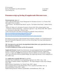
10 Plotting Elementary Functions
Suppose we wish to plot a graph of y =sin3πx for
0 ≤ x ≤ 1. We do this by sampling the function at a
sufficiently large number of points and then joining
up the points (x, y) by straight lines. Suppose we
take N +1 points equally spaced a distance h apart:
>> N =10; h =1/N; x =0:h:1;
defines the set of points x =0,h,2h,...,1 h, 1.
The corresponding y values are computed by
>> y =sin(3*pi*x);
and finally, we can plot the points with
>> plot(x,y)
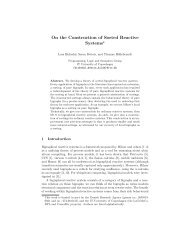
The result is shown in Figure 1, where it is clear
that the value of N is too small.
1
0.8
0.6
0.4
0.2
0
−0.2
−0.4
−0.6
−0.8
−1
0 0.1 0.2 0.3 0.4 0.5 0.6 0.7 0.8 0.9 1
Figure 2: Graph of y =sin3πx for 0 ≤ x ≤ 1using
h =0.01.
10.1 Plotting—Titles & Labels
To put a title and label the axes, we use
>> title(’Graph of y =sin(3pi x)’)
>> xlabel(’x axis’)
>> ylabel(’y-axis’)
The strings enclosed in single quotes, can be anything
of our choosing (it is not straightforward to
get formatted mathematical expressions as in L A TEX).
10.2 Grids
Adottedgridmaybeaddedby
>> grid
This can be removed using either grid again, or
grid off.
1
0.8
0.6
0.4
0.2
0
−0.2
−0.4
−0.6
−0.8
−1
0 0.1 0.2 0.3 0.4 0.5 0.6 0.7 0.8 0.9 1
Figure 1: Graph of y =sin3πx for 0 ≤ x ≤ 1using
h =0.1.
On changing the value of N to 100:
>> N =100; h =1/N; x =0:h:1;
>> y =sin(3*pi*x); plot(x,y)
we get the picture shown in Figure 2.
10.3 Line Styles & Colours
The default is to plot solid lines. A solid white line
is produced by
>> plot(x,y,’w-’)
The third argument is a string whose first character
specifies the colour(optional) and the second the
line style. The options for colours and styles are:
Colours Line Styles
y yellow . point
m magenta o circle
c cyan x x-mark
r red + plus
g green - solid
b blue * star
w white : dotted
k black -. dashdot
-- dashed
6

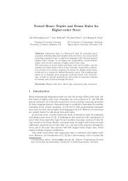
10.4 Multi–plots
Several graphs may be drawn on the same figure as
in
>> plot(x,y,’w-’,x,cos(2*pi*x),’g--’)
A descriptive legend may be included with
>> legend(’Sin curve’,’Cos curve’)
which will give a list of line–styles, as they appeared
in the plot command, followed by a brief description.
Matlab fits the legend in a suitable position,
so as not to conceal the graphs whenever possible.
For further information do help plot etc.
The result of the commands
>> plot(x,y,’w-’,x,cos(2*pi*x),’g--’)
>> legend(’Sin curve’,’Cos curve’)
>> title(’Multi-plot ’)
>> xlabel(’x axis’), ylabel(’y axis’)
>> grid
is shown in Figure 3. The legend may be moved
manually by dragging it with the mouse.
y axis
1
0.8
0.6
0.4
0.2
0
−0.2
−0.4
−0.6
−0.8
Multi−plot
Sin curve
Cos curve
−1
0 0.1 0.2 0.3 0.4 0.5 0.6 0.7 0.8 0.9 1
x axis
Figure 3: Graph of y =sin3πx and y =cos3πx for
0 ≤ x ≤ 1usingh =0.01.
10.6 Hard Copy
To obtain a printed copy on the bubblejet printer:
1. Issue the Matlab command
print -deps fig1
which will save a copy of the image in a file
called fig1.eps (Encapsulated PostScript).
2. Move the mouse pointer into another xterm
window, check that it is looking at the same
directory (pwd) and issue the Unix command
lpr -Pbj
fig1.eps
10.7 Subplot
The graphics window may be split into an m × n
array of smaller windows into which we may plot
one or more graphs. The windows are counted 1
to mn row–wise, starting from the top left. Both
hold and grid work on the current subplot.
>> subplot(221), plot(x,y)
>> xlabel(’x’),ylabel(’sin 3 pi x’)
>> subplot(222), plot(x,cos(3*pi*x))
>> xlabel(’x’),ylabel(’cos 3 pi x’)
>> subplot(223), plot(x,sin(6*pi*x))
>> xlabel(’x’),ylabel(’sin 6 pi x’)
>> subplot(224), plot(x,cos(6*pi*x))
>> xlabel(’x’),ylabel(’cos 6 pi x’)
subplot(221) (or subplot(2,2,1)) specifies that
the window should be split into a 2 × 2 array and
we select the first subwindow.
sin 3 pi x
1
0.5
0
−0.5
−1
0 0.5 1
x
1
cos 3 pi x
1
0.5
0
−0.5
−1
0 0.5 1
x
1
10.5 Hold
Acalltoplot clears the graphics window before
plotting the current graph. This is not convenient
if we wish to add further graphics to the figure at
some later stage. To stop the window being cleared:
sin 6 pi x
0.5
0
−0.5
−1
0 0.5 1
x
cos 6 pi x
0.5
0
−0.5
−1
0 0.5 1
x
>> plot(x,y,’w-’), hold
>> plot(x,y,’gx’), hold off
“hold on” holds the current picture; “hold off”
releases it (but does not clear the window, which
can be done with clg). “hold” on its own toggles
the hold state.
10.8 Zooming
We often need to “zoom in” on some portion of
a plot in order to see more detail. This is easily
achieved using the command
>> zoom
7

Pointing the mouse to the relevant position on the
plot and clicking the left mouse button will zoom
in by a factor of two. This may be repeated to any
desired level.
Clicking the right mouse button will zoom out by
afactoroftwo.
Holding down the left mouse button and dragging
the mouse will cause a rectangle to be outlined. Releasing
the button causes the contents of the rectangle
to fill the window.
zoom off turns off the zoom capability.
Exercise 10.1 Draw graphs of the functions
y = cosx
y = x
for 0 ≤ x ≤ 2 on the same window. Use the zoom
facility to determine the point of intersection of the
two curves (and, hence, the root of x =cosx) to
two significant figures.
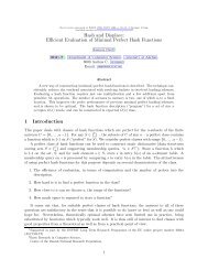
10.9 Controlling Axes
Once a plot has been created in the graphics window
you may wish to change the range of x and y
values shown on the picture.
>> clg, N =100; h =1/N; x =0:h:1;
>> y =sin(3*pi*x); plot(x,y)
>> axis([-0.5 1.5 -1.2 1.2]), grid
The axis command has four parameters, the first
two are the minimum and maximum values of x
to use on the axis and the last two are the minimum
and maximum values of y. Note the square
brackets. The result of these commands is shown in
Figure 4. Look at help axis and experiment with
the commands axis(’equal’), axis(’auto’),
axis(’square’), axis(’normal’), inanyorder.
1
0.8
0.6
0.4
0.2
0
−0.2
−0.4
−0.6
−0.8
−1
−0.5 0 0.5 1 1.5
Figure 4: The effect of changing the axes of a plot.
11 Keyboard Accelerators
One can recall previous Matlab commands by using
the ↑ and ↓ cursor keys. Repeatedly pressing ↑ will
review the previous commands (most recent first)
and, if you want to re-execute the command, simply
press the return key.
To recall the most recent command starting with p,
say, type p at the prompt followed by ↑. Similarly,
typing pr followed by ↑ will recall the most recent
command starting with pr.
Once a command has been recalled, it may be edited
(changed). You can use ← and → to move backwards
and forwards through the line, characters
may be inserted by typing at the current cursor
position or deleted using the Del key. This is most
commonly used when long command lines have been
mistyped or when you want to re–execute a command
that is very similar to one used previously.
The following emacs commands may also be used:
cntrl a
cntrl e
cntrl f
cntrl b
cntrl d
move to start of line
move to end of line
move forwards one character
move backwards one character
delete character under the cursor
Once you have the command in the required form,
press return.
Exercise 11.1 Type in the commands
>> x =-1:0.1:1;
>> plot(x,sin(pi*x),’w-’)
>> hold on
>> plot(x,cos(pi*x),’r-’)
Now use the cursor keys with suitable editing to execute:
>> x =-1:0.05:1;
>> plot(x,sin(2*pi*x),’w-’)
>> plot(x,cos(2*pi*x),’r-.’), hold off
12 Copying to and from Emacs
There are many situations where one wants to copy
the output resulting from a Matlab command (or
commands) into a file being edited in Emacs. The
rules are the same as for copying text in an Emacs
window.
In order to carry out the following exercise, you
should have Matlab running in one window and
Emacs running in another.
To copy material from Matlab into Emacs: ( l means
click Left Mouse Button, etc)
8

Select the material to copy: l on the start of the
material you want in the Matlab window, r at the
end then move the mouse into the Emacs window
and l at the location you want the text to appear.
Finally, click the m .
The process for copying commands from an emacs
file into Matlab is entirely similar, except that you
can only copy material to the prompt line. You
may copy as many lines as you want.
Exercise 12.1
1. Copy the file
∼
dfg/NAP/Matlab/CopyExercise.m
into your own area:
∼
dfg/NAP/Matlab/CopyExercise.m .
Load the file into emacs. You should also have
Matlab running in another xterm window.
2. Copy the commands one at a time from the
file into Matlab.
3. Type CopyExercise at the Matlab prompt—
you should see the results of the commands
being executed.
4. Type echo on at the Matlab prompt and then
CopyExercise—you should see the commands
as well as the results. echo off will switch
off echoing.
13 Script Files
The last part of Exercise 12.1 introduced the idea
of a script file. This is a normal ASCII (text) file
that contains Matlab commands. It is essential
that the file name should have an extension .m (e.g.
Exercise4.m) and, for this reason, they are commonly
known as m-files. The commands in this file
may then be executed using
>> Exercise4
Note: this command does not include the file name
extension .m.
It is only the output from the commands (and not
the commands themselves) that are displayed on
the screen. To see the commands:
>> echo on
and echo off will turn echoing off.
Anytextthatfollows% on a line is ignored. The
main purpose of this facility is to enable comments
to be included in the file to describe its purpose.
To see what m-files you have in your current directory,
use
>> what
Exercise 13.1 1. Type in the commands from
§10.7intoafilecalledexsub.m.
2. Use what to check that the file is in the correct
area.
3. Use the command type exsub to see the contents
of the file.
4. Execute these commands.
See §20 for the related topic of function files.
14 Products, Division & PowersofVectors
14.1 Scalar Product (*)
We shall describe two ways in which a meaning may
be attributed to the product of two vectors. In both
cases the vectors concerned must have the same
length.
The first product is the standard scalar product.
Suppose that u and v are two vectors of length n,
u being a row vector and v a column vector:
u =[u 1 ,u 2 ,...,u n ] , v = ⎢
⎣
⎡
v 1
v 2
.
v n
⎤
⎥
⎦ .
The scalar product is defined by multiplying the
corresponding elements together and adding the results
to give a single number (scalar).
n∑
u v = u i v i .
i=1
For example, if u =[10, 11, 12], and v = ⎣
then n =3and
⎡
20
21
22
u v =10× 20 + ( 11) × ( 21) + 12 × ( 22) = 167.
We can perform this product in Matlab by
>> u =[ 10, -11, 12], v =[20; -21; -22]
>> prod =u*v % row times column vector
Suppose we also define a row vector w and a column
vector z by
>> w =[2, 1, 3], z =[7; 6; 5]
w =
2 1 3
z =
7
6
5
and we wish to form the scalar products of u with
w and v with z.
⎤
⎦
9

u*w
??? Error using ==> *
Inner matrix dimensions must agree.
an error results because w is not a column vector.
Recall from page 5 that transposing (with ’) turns
column vectors into row vectors and vice versa.
So, to form the scalar product of two row vectors
or two column vectors,
>> u*w’ % u & w are row vectors
ans =
45
>> u*u’ % u is a row vector
ans =
365
>> v’*z % v & z are column vectors
ans =
-96
We shall refer to the Euclidean length of a vector as
the norm of a vector; it is denoted by the symbol
‖u‖ and defined by
∑
‖u‖ = √ n |u i | 2 ,
i=1
where n is its dimension. This can be computed in
Matlab in one of two ways:
>> [ sqrt(u*u’), norm(u)]
ans =
19.1050 19.1050
where norm is a built–in Matlab function that accepts
a vector as input and delivers a scalar as output.
It can also be used to compute other norms:
help norm.
Exercise 14.1 The angle, θ, between two column
vectors x and y is defined by
cos θ =
x′ y
‖x‖ ‖y‖ .
Use this formula to determine the cosine of the angle
between
x =[1, 2, 3] ′ and y =[3, 2, 1] ′ .
Hence find the angle in degrees.
14.2 Dot Product (.*)
The second way of forming the product of two vectors
of the same length is known as the Hadamard
product. It is not often used in Mathematics but
is an invaluable Matlab feature. It involves vectors
of the same type. If u and v are two vectors of the
same type (both row vectors or both column vectors),
the mathematical definition of this product,
which we shall call the dot product, isthevector
having the components
u · v =[u 1 v 1 ,u 2 v 2 ,...,u n v n ].
The result is a vector of the same length and type
as u and v. Thus, we simply multiply the corresponding
elements of two vectors.
In Matlab, the product is computed with the operator
.* and, using the vectors u, v, w, z defined
on page 9,
>> u.*w
ans =
20 -11 36
>> u.*v’
ans =
200 231 -264
>> v.*z, u’.*v
ans =
140 -126 -110
ans =
200 231 -264
Example 14.1 Tabulate the function y = x sin πx
for x =0, 0.25,...,1.
It is easier to deal with column vectors so we first
define a vector of x-values: (see Transposing: §8.4)
>> x =(0:0.25:1)’;
To evaluate y we have to multiply each element of
the vector x by the corresponding element of the
vector sin πx:
x × sin πx = x sin πx
0 × 0= 0
0.2500 × 0.7071 = 0.1768
0.5000 × 1.0000 = 0.5000
0.7500 × 0.7071 = 0.5303
1.0000 × 0.0000 = 0.0000
To carry this out in Matlab:
>> y =x.*sin(pi*x)
y =
0
0.1768
0.5000
0.5303
0.0000
Note: a) the use of pi, b)x and sin(pi*x) are both
column vectors (the sin function is applied to each
element of the vector). Thus, the dot product of
these is also a column vector.
10

14.3 Dot Division of Arrays (./)
There is no mathematical definition for the division
of one vector by another. However, in Matlab, the
operator ./ is defined to give element by element
division—it is therefore only defined for vectors of
thesamesizeandtype.
>> a =1:5, b =6:10, a./b
a =
1 2 3 4 5
b =
6 7 8 9 10
ans =
0.1667 0.2857 0.3750 0.4444 0.5000
>> a./a
ans =
1 1 1 1 1
>> c =-2:2, a./c
c =
-2 -1 0 1 2
Warning: Divide by zero
ans =
-0.5000 -2.0000 Inf 4.0000 2.5000
The previous calculation required division by 0—
notice the Inf, denoting infinity, in the answer.
>> a.*b -24, ans./c
ans =
-18 -10 0 12 26
Warning: Divide by zero
ans =
9 10 NaN 12 13
Here we are warned about 0/0—giving a NaN (Not
aNumber).
Example 14.2 Estimate the limit
sin πx
lim
x→0 x .
The idea is to observe the behaviour of the ratio
sin πx
x
for a sequence of values of x that approach
zero. Suppose that we choose the sequence defined
by the column vector
>> x =[0.1; 0.01; 0.001; 0.0001]
then
>> sin(pi*x)./x
ans =
3.0902
3.1411
3.1416
3.1416
which suggests that the values approach π. Toget
a better impression, we subtract the value of π from
each entry in the output and, to display more decimal
places, we change the format
>> format long
>> ans -pi
ans =
-0.05142270984032
-0.00051674577696
-0.00000516771023
-0.00000005167713
Can you explain the pattern revealed in these numbers?
We also need to use ./ to compute a scalar divided
by a vector:
>> 1/x
??? Error using ==> /
Matrix dimensions must agree.
>> 1./x
ans =
10 100 1000 10000
so 1./x works, but 1/x does not.
14.4 Dot Power of Arrays (.^)
To square each of the elements of a vector we could,
for example, do u.*u. However, a neater way is to
use the .^ operator:
>> u.^2
ans =
100 121 144
>> u.*u
ans =
100 121 144
>> u.^4
ans =
10000 14641 20736
>> v.^2
ans =
400
441
484
>> u.*w.^(-2)
ans =
2.5000 -11.0000 1.3333
Recall that powers (.^ in this case) are done first,
before any other arithmetic operation.
15 Examples in Plotting
Example 15.1 Draw graphs of the functions
i) y = sin x ii) u = 1 + x
x (x 1) 2
iii) v = x2 +1
x 2 4
iv) w = (10 x)1/3 2
(4 x 2 ) 1/2
for 0 ≤ x ≤ 10.
11

x =0:0.1:10;
>> y =sin(x)./x;
>> subplot(221), plot(x,y), title(’(i)’)
Warning: Divide by zero
>> u =1./(x-1).^2 + x;
>> subplot(222),plot(x,u), title(’(ii)’)
Warning: Divide by zero
>> v =(x.^2+1)./(x.^2-4);
>> subplot(223),plot(x,v),title(’(iii)’)
Warning: Divide by zero
>> w =((10-x).^(1/3)-1)./sqrt(4-x.^2);
Warning: Divide by zero
>> subplot(224),plot(x,w),title(’(iv)’)
and
z =sin 2 πx/(x 2 +3)
for x = 0, 0.2,...,10. Hence, tabulate the
function
w = (x2 +3)sinπx 2 sin 2 πx
(x 2 .
+3)
Plot a graph of w over the range 0 ≤ x ≤ 10.
16 Matrices—Two–Dimensional
Arrays
1
0.5
0
−0.5
0 5 10
20
10
0
−10
−20
0 5 10
(i)
(iii)
150
100
50
(ii)
0
0 5 10
2
1.5
1
0.5
(iv)
0
0 5 10
Row and Column vectors are special cases of matrices.
An m × n matrix is a rectangular array of numbers
having m rows and n columns. It is usual in a
mathematical setting to include the matrix in either
round or square brackets—we shall use square ones.
For example, when m =2,n =3wehavea2× 3
matrix such as
[ ]
5 7 9
A =
1 3 7
To enter such an matrix into Matlab we type it in
row by row using the same syntax as for vectors:
Note the repeated use of the “dot” operators.
Experiment with changing the axes (page 8), grids
(page 6)and hold(page 7).
>> subplot(222),axis([0 10 0 10])
>> grid
>> grid
>> hold on
>> plot(x,v,’--’), hold off, plot(x,y,’:’)
Exercise 15.1 Enter the vectors
into Matlab.
U =[6, 2, 4], V =[3, 2, 3, 0],
⎡ ⎤ ⎡ ⎤
3
3
W = ⎢ 4
⎥
⎣ 2 ⎦ , Z = ⎢ 2
⎥
⎣ 2 ⎦
6
7
1. Which of the products
U*V, V*W, U*V’, V*W’, W*Z’, U.*V
U’*V, V’*W, W’*Z, U.*W, W.*Z, V.*W
is legal? State whether the legal products are
row or column vectors and give the values of
the legal results.
2. Tabulate the functions
y =(x 2 +3)sinπx 2
>> A =[5 7 9
1 -3 -7]
A =
5 7 9
1 -3 -7
Rows may be separated by semi-colons rather than
a new line:
>> B = [-1 2 5; 9 0 5]
B =
-1 2 5
9 0 5
>> C =[0, 1; 3, -2; 4, 2]
C =
0 1
3 -2
4 2
>> D =[1:5; 6:10; 11:2:20]
D =
1 2 3 4 5
6 7 8 9 10
11 13 15 17 19
So A and B are 2 × 3 matrices, C is 3 × 2andD is
3 × 5.
In this context, a row vector is a 1 × n matrix and
a column vector a m × 1matrix.
12

16.1 Size of a matrix
We can get the size (dimensions) of a matrix with
the command size
>> size(A), size(x)
ans =
2 3
ans =
3 1
>> size(ans)
ans =
1 2
So A is 2 × 3andx is 3 × 1 (a column vector). The
last command size(ans) shows that the value returned
by size is itself a 1 × 2 matrix (a row vector).
We can save the results for use in subsequent
calculations.
>> [r c] =size(A’), S =size(A’)
r =
3
c =
2
S =
3 2
16.2 Transpose of a matrix
Transposing a vector changes it from a row to a
column vector and vice versa (see §8.4). The extension
of this idea to matrices is that transposing
interchanges rows with the corresponding columns:
the 1st row becomes the 1st column, and so on.
>> D, D’
D =
1 2 3 4 5
6 7 8 9 10
11 13 15 17 19
ans =
1 6 11
2 7 13
3 8 15
4 9 17
5 10 19
>> size(D), size(D’)
ans =
3 5
ans =
5 3
16.3 Special Matrices
Matlab provides a number of useful built–in matrices
of any desired size.
ones(m,n) gives an m × n matrix of 1’s,
>> P =ones(2,3)
P =
1 1 1
1 1 1
zeros(m,n) gives an m × n matrix of 0’s,
>> Z =zeros(2,3), zeros(size(P’))
Z =
0 0 0
0 0 0
ans =
0 0
0 0
0 0
The second command illustrates how we can construct
a matrix based on the size of an existing one.
Try ones(size(D)).
An n × n matrix that has the same number of rows
and columns and is called a square matrix.
A matrix is said to be symmetric if it is equal to
its transpose (i.e. it is unchanged by transposition):
>> S =[2 -1 0; -1 2 -1; 0 -1 2],
S =
2 -1 0
-1 2 -1
0 -1 2
>> St =S’
St =
2 -1 0
-1 2 -1
0 -1 2
>> S-St
ans =
0 0 0
0 0 0
0 0 0
16.4 The Identity Matrix
The n × n identity matrix is a matrix of zeros
except for having ones along its leading diagonal
(top left to bottom right). This is called eye(n) in
Matlab (since mathematically it is usually denoted
by I).
>> I =eye(3), x =[8; -4; 1], I*x
I =
1 0 0
0 1 0
0 0 1
x =
8
-4
1
ans =
8
13

-4
1
Notice that multiplying the 3 × 1 vector x by the
3 × 3identityI has no effect (it is like multiplying
anumberby1).
16.5 Diagonal Matrices
A diagonal matrix is similar to the identity matrix
except that its diagonal entries are not necessarily
equal to 1. ⎡
⎤
3 0 0
D = ⎣ 0 4 0 ⎦
0 0 2
is a 3 × 3 diagonal matrix. To construct this in
Matlab, we could either type it in directly
>> D = [-3 0 0; 0 4 0; 0 0 2]
D =
-3 0 0
0 4 0
0 0 2
but this becomes impractical when the dimension is
large (e.g. a 100 × 100 diagonal matrix). We then
use the diag function.We first define a vector d,
say, containing the values of the diagonal entries
(in order) then diag(d) gives the required matrix.
>> d =[-3 4 2], D =diag(d)
d =
-3 4 2
D =
-3 0 0
0 4 0
0 0 2
On the other hand, if A is any matrix, the command
diag(A) extracts its diagonal entries:
>> F = [0 1 8 7; 3 -2 -4 2; 4 2 1 1]
F =
0 1 8 7
3 -2 -4 2
4 2 1 1
>> diag(F)
ans =
0
-2
1
Notice that the matrix does not have to be square.
16.6 Building Matrices
It is often convenient to build large matrices from
smaller ones:
>> C=[0 1; 3 -2; 4 2]; x=[8;-4;1];
>> G =[C x]
G =
0 1 8
3 -2 -4
4 2 1
>> A, B, H =[A; B]
A =
5 7 9
1 -3 -7
B =
-1 2 5
9 0 5
ans =
5 7 9
1 -3 -7
-1 2 5
9 0 5
so we have added an extra column (x) toC in order
to form G and have stacked A and B on top of each
other to form H.
>> J =[1:4; 5:8; 9:12; 20 0 5 4]
J =
1 2 3 4
5 6 7 8
9 10 11 12
20 0 5 4
>> K =[ diag(1:4) J; J’ zeros(4,4)]
K =
1 0 0 0 1 2 3 4
0 2 0 0 5 6 7 8
0 0 3 0 9 10 11 12
0 0 0 4 20 0 5 4
1 5 9 20 0 0 0 0
2 6 10 0 0 0 0 0
3 7 11 5 0 0 0 0
4 8 12 4 0 0 0 0
The command spy(K) will produce a graphical display
of the location of the nonzero entries in K (it
will also give a value for nz—the number of nonzero
entries):
>> spy(K), grid
16.7 Tabulating Functions
This has been addressed in earlier sections but we
are now in a position to produce a more suitable
table format.
Example 16.1 Tabulate the functions y =4sin3x
and u =3sin4x for x =0, 0.1, 0.2,...,0.5.
>> x =0:0.1:0.5;
>> y =4*sin(3*x); u =3*sin(4*x);
14

[ x’ y’ u’]
ans =
0 0 0
0.1000 1.1821 1.1683
0.2000 2.2586 2.1521
0.3000 3.1333 2.7961
0.4000 3.7282 2.9987
0.5000 3.9900 2.7279
Note the use of transpose (’) to get column vectors.
(we could replace the last command by [x; y; u;]’)
Wecouldalsohavedonethismoredirectly:
>> x =(0:0.1:0.5)’;
>> [x 4*sin(3*x) 3*sin(4*x)]
16.8 Extracting Bits of Matrices
We may extract sections from a matrix in much the
same way as for a vector (page 4).
Each element of a matrix is indexed according to
which row and column it belongs to. The entry in
the ith row and jth column is denoted mathematically
by A i,j and, in Matlab, by A(i,j). So
>> J
J =
1 2 3 4
5 6 7 8
9 10 11 12
20 0 5 4
>> J(1,1)
ans =
1
>> J(2,3)
ans =
7
>> J(4,3)
ans =
5
>> J(4,5)
??? Index exceeds matrix dimensions.
>> J(4,1) =J(1,1) + 6
J =
1 2 3 4
5 6 7 8
9 10 11 12
7 0 5 4
>> J(1,1) =J(1,1) - 3*J(1,2)
J =
-5 2 3 4
5 6 7 8
9 10 11 12
7 0 5 4
In the following examples we extract i) the 3rd column,
ii) the 2nd and 3rd columns, iii) the 4th row,
and iv) the “central” 2 × 2matrix.See§8.1.
>> J(:,3) % 3rd column
ans =
3
7
11
5
>> J(:,2:3) % columns 2 to 3
ans =
2 3
6 7
10 11
0 5
>> J(4,:) % 4th row
ans =
7 0 5 4
>> J(2:3,2:3) % rows 2 to 3 & cols 2 to 3
ans =
6 7
10 11
Thus, : on its own refers to the entire column or
row depending on whether it is the first or the second
index.
16.9 Dot product of matrices (.*)
The dot product works as for vectors: corresponding
elements are multiplied together—so the matrices
involved must have the same size.
>> A, B
A =
5 7 9
1 -3 -7
B =
-1 2 5
9 0 5
>> A.*B
ans =
-5 14 45
9 0 -35
>> A.*C
??? Error using ==> .*
Matrix dimensions must agree.
>> A.*C’
ans =
0 21 36
1 6 -14
16.10 Matrix–vector products
We turn next to the definition of the product of a
matrix with a vector. This product is only defined
for column vectors that have the same number
of entries as the matrix has columns. So, if A is an
m × n matrix and x is a column vector of length n,
then the matrix–vector Ax is legal.
15

An m × n matrix times an n × 1matrix⇒ a m × 1
matrix.
We visualise A as being made up of m row vectors
stacked on top of each other, then the product corresponds
to taking the scalar product (See §14.1)
of each row of A with the vector x: The result is a
column vector with m entries.
Ax =
=
=
[
5 7 9
1 3 7
] ⎡ ⎢ ⎣
8
4
1
⎤
⎥
⎦
[
]
5 × 8+7× ( 4)+9× 1
1 × 8+( 3)× ( 4)+( 7 )× 1
[ ] 21
13
It is somewhat easier in Matlab:
>> A =[5 7 9; 1 -3 -7]
A =
5 7 9
1 -3 -7
>> x =[8; -4; 1]
x =
8
-4
1
>> A*x
ans =
21
13
(m× n) times(n ×1) ⇒ (m × 1).
of A with the jth column of B. The product is an
m × p matrix:
(m× n) times(n ×p) ⇒ (m × p).
Check that you understand what is meant by working
out the following examples by hand and comparing
with the Matlab answers.
>> A =[5 7 9; 1 -3 -7]
A =
5 7 9
1 -3 -7
>> B =[0, 1; 3, -2; 4, 2]
B =
0 1
3 -2
4 2
>> C =A*B
C =
57 9
-37 -7
>> D =B*A
D =
1 -3 -7
13 27 41
22 22 22
>> E =B’*A’
E =
57 -37
9 -7
We see that E = C’ suggesting that
>> x*A
??? Error using ==> *
Inner matrix dimensions must agree.
Unlike multiplication in arithmetic, A*x is not the
same as x*A.
16.11 Matrix–Matrix Products
To form the product of an m × n matrix A and a cp ~dfg/Matlab/fireworks.m .
n×p matrix B, written as AB, we visualise the first
matrix (A) as being composed of m row vectors of
length n stacked on top of each other while the second
(B) is visualised as being made up of p column
vectors of length n:
cp ~dfg/Matlab/comet*.m
then, in Matlab,
>> fireworks
.
⎧⎡
⎤
A graphics window will pop up, in which you should
⎡ ⎤
click the left mouse button on Fire .
⎪⎨
A = m rows ⎢
⎣
⎥
. ⎦ , B = ⎢
⎣ ··· ⎥
⎦,
To end the demo, click on Fire again, then on
⎪⎩
} {{ }
Done .
p columns
The entry in the ith row and jth column of the
product is then the scalarproduct of the ith row
(A*B)’ = B’*A’
Why is B ∗ A a3× 3 matrix while A ∗ B is 2 × 2?
17 Fireworks
As light relief, use your xterm window to copy three
files to your area:
16

18 Loops
There are occasions that we want to repeat a segment
of code a number of different times (such occasions
are less frequent than other programming
languages because of the : notation).
Example 18.1 Draw graphs of sin(nπx) on the interval
1 ≤ x ≤ 1 for n =1, 2,...,8.
We could do this by giving 8 separate plot commands
but it is much easier to use a loop. The
simplest form would be
>> x =-1:.05:1;
>> for n =1:8
subplot(4,2,n), plot(x,sin(n*pi*x))
end
All the commands between the lines starting “for”
and “end” are repeated with n being given the value
1 the first time through, 2 the second time, and so
forth, until n =8. Thesubplot constructs a 4 × 2
array of subwindows and, on the nth time through
the loop, a picture is drawn in the nth subwindow.
The commands
>> F(1) =0; F(2) =1;
>> for i =3:20
F(i) =F(i-1) + F(i-2);
end
>> plot(1:19, F(2:20)./F(1:19),’o’ )
>> hold on
>> plot(1:19, F(2:20)./F(1:19),’-’ )
>> plot([0 20], (sqrt(5)+1)/2*[1,1],’--’)
The last of these commands produced the dashed
horizontal line.
2
1.9
1.8
1.7
1.6
1.5
1.4
1.3
1.2
1.1
1
0 2 4 6 8 10 12 14 16 18 20
>> x =-1:.05:1;
>> for n =1:2:8
subplot(4,2,n), plot(x,sin(n*pi*x))
subplot(4,2,n+1), plot(x,cos(n*pi*x))
end
draw sin nπx and cos nπx for n =1, 3, 5, 7alongside
each other.
We may use any legal variable name as the “loop
counter” (n in the above examples) and it can be
made to run through all of the values in a given
vector (1:8 and 1:2:8 in the examples).
We may also use for loops of the type
>> for counter =[23 11 19 5.4 6]
.......
end
which repeats the code as far as the end with
counter=23 the first time, counter=11 the second
time, and so forth.
Example 18.2 The Fibonnaci sequence starts off
with the numbers 0 and 1, then succeeding terms are
the sum of its two immediate predecessors. Mathematically,
f 1 =0, f 2 =1and
f n = f n 1 + f n 2 , n =3, 4, 5,....
Example 18.3 Produce a list of the values of the
sums
S 20 = 1+ 1
2
+ 1 2 3
+ ···+ 1
2 20 2
S 21 = 1+ 1
2
+ 1 2 3
+ ···+ 1
2 20
+ 1
2 21 2
.
S 100 = 1+ 1
2
+ 1 2 3
+ ···+ 1
2 20
+ 1
2 21
+ ···+ 1
2 100 2
There are a total of 81 sums. The first can be
computed using sum(1./(1:20).^2) (The function
sum with a vector argument sums its components.
See §21.2].) A suitable piece of Matlab code might
be
>> S =zeros(100,1);
>> S(20) =sum(1./(1:20).^2);
>> for n =21:100
>> S(n) =S(n-1) + 1/n^2;
>> end
>> clg; plot(S,’.’,[20 100],[1,1]*pi^2/6,’-’)
>> axis([20 100 1.5 1.7])
>> [ (98:100)’ S(98:100)]
ans =
98.0000 1.6364
99.0000 1.6365
100.0000 1.6366
where a column vector S was created to hold the
Test the assertion that the ratio f n /f n 1 of two successive
values approaches the golden ratio ( √ answers. The first sum was computed directly using
5+1)/2 the sum command then each succeeding sum was
=1.6180 ....
found by adding 1/n 2 to its predecessor. The little
table at the end shows the values of the last three
17

sums—it appears that they are approaching a limit
(the value of the limit is π 2 /6=1.64493 ...).
Exercise 18.1 Repeat Example 18.3 to include 181
sums (i.e. the final sum should include the term
1/200 2 .)
19 Logicals
= =
Matlab represents true and false by means of the
integers 0 and 1.
true =1, false =0
If at some point in a calculation a scalar x, say,has
been assigned a value, we may make certain logical
tests on it:
x 2 is x equal to 2?
x ~= 2 is x not equal to 2?
x > 2 is x greater than 2?
x < 2 is x less than 2?
x >= 2 is x greater than or equal to 2?
x > x =pi
x =
3.1416
>> x ~=3, x ~=pi
ans =
1
ans =
0
When x is a vector or a matrix, these tests are
performed elementwise:
x =
-2.0000 3.1416 5.0000
-1.0000 0 1.0000
>> x == 0
ans =
0 0 0
0 1 0
>> x > 1, x >=-1
ans =
0 1 1
0 0 0
ans =
0 1 1
1 1 1
>> y =x>=-1, x > y
y =
0 1 1
1 1 1
ans =
0 1 1
0 0 0
We may combine logical tests, as in
>> x
x =
-2.0000 3.1416 5.0000
-5.0000 -3.0000 -1.0000
>> x > 3 & x < 4
ans =
0 1 0
0 0 0
>> x > 3 | x -3
ans =
0 1 1
0 1 0
As one might expect, & represents and and (not so
clearly) the vertical bar | means or; also~ means
not as in ~= (not equal), ~(x>0), etc.
>> x > 3 | x ==-3 | x > x, L =x >=0
x =
-2.0000 3.1416 5.0000
-5.0000 -3.0000 -1.0000
L =
0 1 1
0 1 1
>> pos =x.*L
pos =
0 3.1416 5.0000
0 0 0
so the matrix pos contains just those elements of x
that are non–negative.
>> x =0:0.05:6; y =sin(pi*x); Y =(y>=0).*y;
>> plot(x,y,’:’,x,Y,’-’ )
1
0.8
0.6
0.4
0.2
0
−0.2
−0.4
−0.6
−0.8
−1
0 1 2 3 4 5 6
18

19.1 While Loops
There are some occasions when we want to repeat a
section of Matlab code until some logical condition
is satisfied, but we cannot tell in advance how many
times we have to go around the loop. This we can
do with a while...end construct.
Example 19.1 What is the greatest value of n that
canbeusedinthesum
1 2 +2 2 + ···+ n 2
and get a value of less than 100?
>> S =1; n =1;
>> while S+ (n+1)^2 < 100
n =n+1; S =S + n^2;
end
>> [n, S]
ans =
6 91
The lines of code between while and end will only
be executed if the condition S+ (n+1)^2 < 100 is
true.
Exercise 19.1 Replace 100 in the previous example
by 10 and work through the lines of code by
hand. You should get the answers n =2and S =5.
Exercise 19.2 Type the code from Example19.1 into
ascript–filenamedWhileSum.m (See §13.)
A more typical example is
Example 19.2 Find the approximate value of the
root of the equation x =cosx. (See Example 10.1.)
We may do this by making a guess x 1 = π/4, say,
then computing the sequence of values
x n =cosx n 1 , n =2, 3, 4,...
and continuing until the difference between two successive
values |x n x n 1 | is small enough.
Method 1:
>> x = zeros(1,20); x(1) = pi/4;
>> n = 1; d = 1;
>> while d > 0.001
n = n+1; x(n) = cos(x(n-1));
d = abs( x(n) - x(n-1) );
end
n,x
n =
14
x =
Columns 1 through 7
0.7854 0.7071 0.7602 0.7247 0.7487 0.7326 0.7435
Columns 8 through 14
0.7361 0.7411 0.7377 0.7400 0.7385 0.7395 0.7388
Columns 15 through 20
0 0 0 0 0 0
There are a number of deficiencies with this program.
The vector x stores the results of each iteration
but we don’t know in advance how many
there may be. In any event, we are rarely interested
in the intermediate values of x, only the last
one. Another problem is that we may never satisfy
the condition d ≤ 0.001, in which case the program
will run forever—we should place a limit on the
maximum number of iterations.
Incorporating these improvements leads to
Method 2:
>> xold =pi/4; n =1; d =1;
>> while d > 0.001 & n < 20
n =n+1; xnew =cos(xold);
d =abs( xnew - xold );
xold =xnew;
end
>> [n, xnew, d]
ans =
14.0000 0.7388 0.0007
We continue around the loop so long as d>0.001
and n0.0001, and this gives
>> [n, xnew, d]
ans =
19.0000 0.7391 0.0001
from which we may judge that the root required is
x =0.739 to 3 decimal places.
The general form of while statement is
while alogicaltest
Commands to be executed
when the condition is true
end
19.2 if...then...else...end
This allows us to execute different commands depending
on the truth or falsity of some logical tests.
To test whether or not π e is greater than, or equal
to, e π :
>> a =pi^exp(1); c =exp(pi);
>> if a >=c
b =sqrt(a^2 - c^2)
end
so that b is assigned a value only if a ≥ c. Thereis
no output so we deduce that a = π e > if a >=c
b =sqrt(a^2 - c^2)
else
19

= 0
end
b =
0
which ensures that b is always assigned a value and
confirming that a> if a >=c
b =sqrt(a^2 - c^2)
elseif a^c > c^a
b =c^a/a^c
else
b =a^c/c^a
end
b =
0.2347
Exercise 19.3 Which of the above statements assignedavaluetob?
The general form of the if statement is
2. Thefirstlineofthefilemusthavetheformat:
function [list of outputs]
= function name(list of inputs)
For our example, the output (A) is a function
of the three variables (inputs) a, b and c so
the first line should read
function [A] =area(a,b,c)
3. Document the function. That is, describe
briefly the purpose of the function and how it
can be used. These lines should be preceded
by % which signify that they are comment
lines that will be ignored when the function
is evaluated.
4. Finally include the code that defines the function.
This should be interspersed with sufficient
comments to enable another user to understand
the processes involved.
The complete file might look like:
if logical test 1
Commands to be executed if test
1istrue
elseif logical test 2
Commands to be executed if test
2istruebuttest1isfalse
.
end
20 Function m–files
These are a combination of the ideas of script m–
files (§7) and Mathematical functions.
Example 20.1 The area, A, of a triangle with sides
of length a, b and c is given by
A = √ s(s a)(s b)(s c),
where s =(a + b + c)/2. Write a Matlab function
that will accept the values a, b and c as inputs and
return the value os A as output.
The main steps to follow when defining a Matlab
function are:
1. Decide on a name for the function, making
sure that it does not conflict with a name that
is already used by Matlab. In this example
the name of the function is to be area, soits
definition will be saved in a file called area.m
function [A] =area(a,b,c)
% Compute the area of a triangle whose
% sides have length a, b and c.
% Inputs:
% a,b,c: Lengths of sides
% Output:
% A: area of triangle
% Usage:
% Area =area(2,3,4);
% Written by dfg, Oct 14, 1996.
s =(a+b+c)/2;
A =sqrt(s*(s-a)*(s-b)*(s-c));
%%%%%%%%% end of area %%%%%%%%%%%
The command
>> help area
will produce the leading comments from the file:
Compute the area of a triangle whose
sides have length a, b and c.
Inputs:
a,b,c: Lengths of sides
Output:
A: area of triangle
Usage:
Area =area(2,3,4);
Written by dfg, Oct 14, 1996.
To evalute the area of a triangle with side of length
10, 15, 20:
>> Area =area(10,15,20)
Area =
72.6184
20

where the result of the computation is assigned to
the variable Area. The variable s used in the definition
of the function above is a “local variable”:
its value is local to the function and cannot be used
outside:
>> s
??? Undefined function or variable s.
If we were to be interested in the value of s as well
as A, then the first line of the file should be changed
to
function [A,s] =area(a,b,c)
where there are two output variables.
This function can be called in several different ways:
1. No outputs assigned
>> area(10,15,20)
ans =
72.6184
gives only the area (first of the output variables
from the file) assigned to ans; the second
output is ignored.
2. One output assigned
>> Area =area(10,15,20)
Area =
72.6184
again the second output is ignored.
3. Two outputs assigned
>> [Area, hlen] =area(10,15,20)
Area =
72.6184
hlen =
22.5000
Exercise 20.1 In any triangle the sum of the lengths Method 3:
of any two sides cannot exceed the length of the
third side. The function area does not check to
see if this condition is fulfilled (try area(1,2,4)).
Modify the file so that it computes the area only if
the sides satisfy this condition.
20.1 Examples of functions
We revisit the problem of computing the Fibonnaci
sequence defined by f 1 =0,f 2 =1and
f n = f n 1 + f n 2 , n =3, 4, 5,....
We want to construct a function that will return
the nth number in the Fibinnaci sequence f n .
• Input: Integer n
• Output: f n
We shall describe four possible functions and try to
assess which provides the best solution.
Method 1:
File ∼ dfg/Matlab/doc/Fib1.m
function f =Fib1(n)
% Returns the nth number in the
% Fibonacci sequence.
F=zeros(1,n+1);
F(2) =1;
for i =3:n+1
F(i) =F(i-1) + F(i-2);
end
f =F(n);
This code resembles that given in Example 18.2.
We have simply enclosed it in a function m–file and
given it the appropriate header,
Method 2: File ∼ dfg/Matlab/doc/Fib2.m
The first version was rather wasteful of memory—it
saved all the entries in the sequence even though we
only required the last one for output. The second
version removes the need to use a vector.
function f =Fib2(n)
% Returns the nth number in the
% Fibonacci sequence.
if n==1
f = 0;
elseif n==2
f = 1;
else
f1 =0; f2 =1;
for i =2:n-1
f =f1 + f2;
f1=f2; f2 = f;
end
end
File: ∼ dfg/Matlab/doc/Fib3.m
This version makes use of an idea called “recursive
programming”— the function makes calls to itself.
function f =Fib3(n)
% Returns the nth number in the
% Fibonacci sequence.
if n==1
f = 0;
elseif n==2
f = 1;
else
f =Fib3(n-1) + Fib3(n-2);
end
Method 4: File ∼ dfg/Matlab/doc/Fib4.m
The final version uses matrix [ powers. ] The vector y
fn
has two components, y = .
f n+1
21

function f =Fib4(n)
% Returns the nth number in the
% Fibonacci sequence.
A =[0 1;1 1];
y =A^n*[1;0];
f=y(1);
Assessment: One may think that, on grounds of
style, the 3rd is best (it avoids the use of loops) followed
by the second (it avoids the use of a vector).
The situation is much different when it cames to
speed of execution. When n = 20 the time taken
by each of the methods is (in seconds)
Method Time
1 0.0118
2 0.0157
3 36.5937
4 0.0078
It is impractical to use Method 3 for any value of n
much larger than 10 since the time taken by method
3 almost doubles whenever n is increased by just 1.
When n = 150
Method Time
1 0.0540
2 0.0891
3 —
4 0.0106
Clearly the 4th method is much the fastest.
21 Further Built–in Functions
21.1 Rounding Numbers
There are a variety of ways of rounding and chopping
real numbers to give integers. Use the definitions
given in the table in §26 on page 26 in order
to understand the output given below:
>> x =pi*(-1:3), round(x)
x =
-3.1416 0 3.1416 6.2832 9.4248
ans =
-3 0 3 6 9
>> fix(x)
ans =
-3 0 3 6 9
>> floor(x)
ans =
-4 0 3 6 9
>> ceil(x)
ans =
-3 0 4 7 10
>> sign(x), rem(x,3)
ans =
-1 0 1 1 1
ans =
-0.1416 0 0.1416 0.2832 0.4248
Do “help round” for help information.
21.2 The sum Function
The “sum” applied to a vector adds up its components
(as in sum(1:10)) while, for a matrix, it adds
up the components in each column and returns a
row vector. sum(sum(A)) then sums all the entries
of A.
>> A =[1:3; 4:6; 7:9]
A =
1 2 3
4 5 6
7 8 9
>> s =sum(A), ss =sum(sum(A))
s =
12 15 18
ss =
45
>> x =pi/4*(1:3)’;
>> A =[sin(x), sin(2*x), sin(3*x)]/sqrt(2)
>> A =
0.5000 0.7071 0.5000
0.7071 0.0000 -0.7071
0.5000 -0.7071 0.5000
>> s1 =sum(A.^2), s2 =sum(sum(A.^2))
s1 =
1.0000 1.0000 1.0000
s2 =
3.0000
The sums of squares of the entries in each column
of A are equal to 1 and the sum of squares of all the
entries is equal to 3.
>> A*A’
ans =
1.0000 0 0
0 1.0000 0.0000
0 0.0000 1.0000
>> A’*A
ans =
1.0000 0 0
0 1.0000 0.0000
0 0.0000 1.0000
It appears that the products AA ′ and A ′ A are both
equal to the identity:
>> A*A’ - eye(3)
ans =
1.0e-15 *
22

-0.2220 0 0
0 -0.2220 0.0555
0 0.0555 -0.2220
>> A’*A - eye(3)
ans =
1.0e-15 *
-0.2220 0 0
0 -0.2220 0.0555
0 0.0555 -0.2220
This is confirmed since the differences are at round–
off error levels (less than 10 15 ). A matrix with this
property is called an orthogonal matrix.
21.3 max & min
These functions act in a similar way to sum. Ifx is
a vector, then max(x) returns the largest element
in x
This requires random numbers that are integers in
the range 1 to 6. Multiplying each random number
by 6 will give a real number in the range 0 to 6;
rounding these to whole numbers will not be correct
since it will then be possible to get 0 as an answer.
We need to use
floor(1 + 6*rand)
Recall that floor takes the largest integer that
is smaller than a given real number (see Table 1,
page 26).
File: ∼ dfg/Matlab/doc/dice.m
function [d] =dice(n)
% simulates "n" throws of a pair of dice
% Input: n, the number of throws
% Output: an n times 2 matrix, each row
% referring to one throw.
%
>> x =[1.3 -2.4 0 2.3], max(x), max(abs(x)) % Useage: T =dice(3)
x =
1.3000 -2.4000 0 2.3000
ans =
2.3000
ans =
2.4000
>> [m, j] =max(x)
m =
>> dice(3)
ans =
6
2
4
1
3
1
2.3000
>> sum(dice(100))/100
j =
ans =
4
3.8500 3.4300
d =floor(1 + 6*rand(n,2));
%% end of dice
When we ask for two outputs, the first gives us the
maximum entry and the second the index of the
maximum element.
For a matrix, A, max(A) returns a row vector containing
the maximum element from each column.
Thus to find the largest element in A we have to
use max(max(A)).
21.4 Random Numbers
The function rand(m,n) produces an m×n matrix
of random numbers, each of which is in the range
0to1. rand on its own produces a single random
number.
>> y =rand, Y =rand(2,3)
y =
0.9191
Y =
0.6262 0.1575 0.2520
0.7446 0.7764 0.6121
Repeating these commands will lead to different answers.
Example: Write a function–file that will simulate
n throws of a pair of dice.
The last command gives the average value over 100
throws (it should have the value 3.5).
21.5 find for vectors
The function “find” returns a list of the positions
(indices) of the elements of a vector satisfying a
given condition. For example,
>> x =-1:.05:1;
>> y =sin(3*pi*x).*exp(-x.^2); plot(x,y,’:’)
>> k =find(y > 0.2)
k =
Columns 1 through 12
9 10 11 12 13 22 23 24 25 26 27 36
Columns 13 through 15
37 38 39
>> hold on, plot(x(k),y(k),’o’)
>> km =find( x>0.5 & y> plot(x(km),y(km),’-’)
23

1
0.8
0.6
0.4
0.2
0
−0.2
−0.4
−0.6
−0.8
−1
−1 −0.8 −0.6 −0.4 −0.2 0 0.2 0.4 0.6 0.8 1
21.6 find for matrices
The find–function operates in much the same way
for matrices:
>> A = [ -2 3 4 4; 0 5 -1 6; 6 8 0 1]
A =
-2 3 4 4
0 5 -1 6
6 8 0 1
>> k = find(A==0)
k =
2
9
Thus, we find that A haselementsequalto0inpositions
2 and 9. To interpret this result we have to
recognise that “find” firstreshapesA into a column
vector—this is equivalent to numbering the
elements of A by columns as in
>> n =find(A > A(n)
ans =
-2
0
-1
0
1 4 7 10
2 5 8 11
3 6 9 12
Thus, n gives a list of the locations of the entries in
A that are ≤ 0andthenA(n) gives us the values of
the elements selected.
>> m =find( A’ ==0)
m =
5
11
Since we are dealing with A’, theentriesarenumbered
by rows.
22 Plotting Surfaces
A surface is defined mathematically by a function
f(x, y)—corresponding to each value of (x, y) we
compute the height of the function by
z = f(x, y).
In order to plot this we have to decide on the ranges
of x and y—suppose 2 ≤ x ≤ 4and1≤ y ≤ 3. This
givesusasquareinthe(x, y)–plane. Next, we need
to choose a grid on this domain; Figure 5 shows the
grid with intervals 0.5 in each direction. Finally, we
3
2.5
2
1.5
1
2 2.5 3 3.5 4
Figure 5: An example of a 2D grid
have to evaluate the function at each point of the
grid and “plot” it.
Suppose we choose a grid with intervals 0.5 in each
direction for illustration. The x–andy–coordinates
of the grid lines are
x =2:0.5:4; y =1:0.5:3;
in Matlab notation.
meshgrid:
We construct the grid with
>> [X,Y] = meshgrid(2:.5:4, 1:.5:3);
>> X
X =
2.0000 2.5000 3.0000 3.5000 4.0000
2.0000 2.5000 3.0000 3.5000 4.0000
2.0000 2.5000 3.0000 3.5000 4.0000
2.0000 2.5000 3.0000 3.5000 4.0000
2.0000 2.5000 3.0000 3.5000 4.0000
>> Y
Y =
1.0000 1.0000 1.0000 1.0000 1.0000
1.5000 1.5000 1.5000 1.5000 1.5000
2.0000 2.0000 2.0000 2.0000 2.0000
2.5000 2.5000 2.5000 2.5000 2.5000
3.0000 3.0000 3.0000 3.0000 3.0000
If we think of the ith point along from the left and
the jth point up from the bottom of the grid) as corresponding
to the (i, j)th entry in a matrix, then (X(i,j),
24

Y(i,j)) are the coordinates of the point. We then need
to evaluate the function f using X and Y in place of x
and y, respectively.
0.1
Example 22.1 Plot the surface defined by the function
0.05
f(x, y) =(x 3) 2 (y 2) 2
0
for 2 ≤ x ≤ 4 and 1 ≤ y ≤ 3.
−0.05
>> [X,Y] = meshgrid(2:.2:4, 1:.2:3);
>> Z = (X-3).^2-(Y-2).^2;
>> mesh(X,Y,Z)
>> title(’Saddle’), xlabel(’x’),ylabel(’y’)
−0.1
2
1
0
y
−1
−2
−2
−1
x
0
1
2
2
Saddle
1.5
1
1
0.5
0.5
y
0
0
−0.5
−0.5
−1
−1
3
−1.5
2.5
2
3.5
3
1.5
2.5
y
1 2
x
Figure 6: Plot of Saddle function.
4
−2
−2 −1.5 −1 −0.5 0 0.5 1 1.5 2
x
Figure 7: “mesh” and“contour” plots.
2
Example 22.2 Plot the surface defined by the function
f = xye 2(x2 +y 2 )
on the domain 2 ≤ x ≤ 2, 2 ≤ y ≤ 2. Find the
values and locations of the maxima and minima of the
function.
>> [X,Y] = meshgrid(-2:.1:2,-2:.2:2);
>> f = -X.*Y.*exp(-2*(X.^2+Y.^2));
>> mesh(X,Y,f), xlabel(’x’), ylabel(’y’), grid
>> contour(X,Y,f)
>> xlabel(’x’), ylabel(’y’), grid, hold on
To locate the maxima of the “f” values on the grid:
>> fmax = max(max(f))
fmax =
0.0886
>> kmax = find(f==fmax)
kmax =
323
539
>> Pos = [X(kmax), Y(kmax)]
Pos =
-0.5000 0.6000
0.5000 -0.6000
>> plot(X(kmax),Y(kmax),’*’)
>> text(X(kmax),Y(kmax),’ Maximum’)
y
1.5
1
0.5
0
−0.5
−1
−1.5
Maximum
Maximum
−2
−2 −1.5 −1 −0.5 0 0.5 1 1.5 2
x
Figure 8: contour plot showing maxima.
23 Timing
Matlab allows the timing of sections of code by providing
the functions tic and toc. tic switches on a
stopwatch while toc stops it and returns the CPU time
(Central Processor Unit) in seconds. The timings will
vary depending on the model of computer being used
and its current load.
>> tic,for j=1:1000,x = pi*R(3);end,toc
elapsed_time = 0.5110
>> tic,for j=1:1000,x=pi*R(3);end,toc
elapsed_time = 0.5017
25

tic,for j=1:1000,x=R(3)/pi;end,toc
elapsed_time = 0.5203
>> tic,for j=1:1000,x=pi+R(3);end,toc
elapsed_time = 0.5221
>> tic,for j=1:1000,x=pi-R(3);end,toc
elapsed_time = 0.5154
>> tic,for j=1:1000,x=pi^R(3);end,toc
elapsed_time = 0.6236
24 On–line Documentation
In addition to the on–line help facility, there is a hypertext
browsing system giving details of (most) commands
and some examples. This is accessed by
>> doc
which brings up the Netscape document previewer (and
allows for “surfing the internet superhighway”—the World
Wide Web (WWW). It is connected to a worldwide system
which, given the appropriate addresses, will provide
information on almost any topic).
Words that are underlined in the browser may be clicked
on with LB and lead to either a further subindex or a
help page.
Scroll down the page shown and click on general which
will yake you to “General Purpose Commands”; click on
clear. This will describe how you can clear a variable’s
value from memory.
You may then either click the “Table of Contents” which
takes you back to the start, “Index” or the Back button
at the lower left corner of the window which will
take you back to the previous screen.
To access other “home pages”, click on Open at the
bottom of the window and, in the “box” that will open
up, type
http://www.mcs.dundee.ac.uk
or
http://www.mcs.dundee.ac.uk/~dfg/homepage.html
Further information regarding the commands listed in
this section may then be obtained by using:
>> help topic
try, for example,
>> help help
abs Absolute value
sqrt Square root function
sign Signum function
conj Conjugate of a complex number
imag Imaginary part of a complex
number
real Real part of a complex number
angle Phase angle of a complex number
cos Cosine function
sin Sine function
tan Tangent function
exp Exponential function
log Natural logarithm
log10 Logarithm base 10
cosh Hyperbolic cosine function
sinh Hyperbolic sine function
tanh Hyperbolic tangent function
acos Inverse cosine
acosh Inverse hyperbolic cosine
asin Inverse sine
asinh Inverse hyperbolic sine
atan Inverse tan
atan2 Two–argument form of inverse
tan
atanh Inverse hyperbolic tan
round Round to nearest integer
floor Round towards minus infinity
fix Round towards zero
ceil Round towards plus infinity
rem Remainder after division
Table 1: Elementary Functions
25 Demos
Demonstrations are valuable since they give an indication
of Matlabs capabilities.
>> demo
Warning: this will clear the values of all current variables.
Click on Continue ,then Matlab/Visit ,
Visualization/Select , XY plots ,etc.
26 Command Summary
The command
>> help
will give a list of categories for which help is available
(e.g. matlab/general covers the topics listed in Table 2.
26

Managing commands and functions.
help On-line documentation.
doc Load hypertext documentation.
what Directory listing of M-, MATand
MEX-files.
type List M-file.
lookfor Keyword search through the
HELP entries.
which Locate functions and files.
demo Run demos.
Managing variables and the workspace.
who List current variables.
whos List current variables, long form.
load Retrieve variables from disk.
save Save workspace variables to disk.
clear Clear variables and functions
from memory.
size Size of matrix.
length Length of vector.
disp Display matrix or text.
Working with files and the operating system.
cd Change current working
directory.
dir Directory listing.
delete Delete file.
! Execute operating system
command.
unix Execute operating system command
& return result.
diary Save text of MATLAB session.
Controlling the command window.
cedit Set command line edit/recall facility
parameters.
clc Clear command window.
home Send cursor home.
format Set output format.
echo Echo commands inside script
files.
more Control paged output in command
window.
Quitting from MATLAB.
quit Terminate MATLAB.
Table 2: General purpose commands.
Matrix analysis.
cond Matrix condition number.
norm Matrix or vector norm.
rcond LINPACK reciprocal condition
estimator.
rank Number of linearly independent
rows or columns.
det Determinant.
trace Sum of diagonal elements.
null Null space.
orth Orthogonalization.
rref Reduced row echelon form.
Linear equations.
\ and / Linear equation solution; use
“help slash”.
chol Cholesky factorization.
lu Factors from Gaussian
elimination.
inv Matrix inverse.
qr Orthogonal- triangular
decomposition.
qrdelete Delete a column from the QR
factorization.
qrinsert Insert a column in the QR
factorization.
nnls Non–negative least- squares.
pinv Pseudoinverse.
lscov Least squares in the presence of
known covariance.
Eigenvalues and singular values.
eig Eigenvalues and eigenvectors.
poly Characteristic polynomial.
polyeig Polynomial eigenvalue problem.
hess Hessenberg form.
qz Generalized eigenvalues.
rsf2csf Real block diagonal form to complex
diagonal form.
cdf2rdf Complex diagonal form to real
block diagonal form.
schur Schur decomposition.
balance Diagonal scaling to improve
eigenvalue accuracy.
svd Singular value decomposition.
Matrix functions.
expm Matrix exponential.
expm1 M- file implementation of expm.
expm2 Matrix exponential via Taylor
series.
expm3 Matrix exponential via eigenvalues
and eigenvectors.
logm Matrix logarithm.
sqrtm Matrix square root.
funm Evaluate general matrix function.
Table 3: Matrix functions—numerical linear algebra.
27

Graphics & plotting.
figure Create Figure (graph window).
clf Clear current figure.
close Close figure.
subplot Create axes in tiled positions.
axis Control axis scaling and
appearance.
hold Hold current graph.
figure Create figure window.
text Create text.
print Save graph to file.
plot Linear plot.
loglog Log-log scale plot.
semilogx Semi-log scale plot.
semilogy Semi-log scale plot.
Specialized X-Y graphs.
polar Polar coordinate plot.
bar Bar graph.
stem Discrete sequence or ”stem” plot.
stairs Stairstep plot.
errorbar Error bar plot.
hist Histogram plot.
rose Angle histogram plot.
compass Compass plot.
feather Feather plot.
fplot Plot function.
comet Comet-like trajectory.
Graph annotation.
title Graph title.
xlabel X-axis label.
ylabel Y-axis label.
text Text annotation.
gtext Mouse placement of text.
grid Grid lines.
contour Contour plot.
mesh 3-D mesh surface.
surf 3-D shaded surface.
waterfall Waterfall plot.
view 3-D graph viewpoint
specification.
zlabel Z-axis label for 3-D plots.
gtext Mouse placement of text.
grid Grid lines.
Table 4: Graphics & plot commands.
28

Index
=, 18, 20
%, 9,20
’, 5
.’, 5
.*, 10
./, 11
.^, 11
:, 4,5,15
;, 3
abs, 26
accelerators
keyboard, 8
and, 18
angle, 26
ans, 3
array, 12
axes,8,12
axis, 8
auto, 8
normal, 8
square, 8
browser, 26
ceil, 26
colon notation, 4, 15
column vectors, 5
comment (%), 9, 20
complex
conjugate transpose, 5
numbers, 5
complex numbers, 3
components of a vector, 4
conj, 26
contour, 25
copying output, 8
cos, 26
CPU, 25
cursor keys, 8
demo, 26
diag, 14
diary, 5
dice, 23
divide
dot, 11
documentation, 26
dot
divide ./, 11
power .^, 11
product .*, 10, 15
echo, 9
elementary functions, 3
eye, 13
false, 18
Fibonnaci, 17, 21
file
function, 20
script, 9
find, 23,24
fix, 26
floor, 26
floor, 23
for
loop, 17
format, 2
long, 11
function m–files, 20
functions
elementary, 3
trigonometric, 3
graphs, see plotting
grid, 6, 12, 24
hard copy, 7
help, 2,20
hold, 7,12
home page, 26
if statement, 19
imag, 26
keyboard accelerators, 8
labels for plots, 6
legend, 7
length of a vector, 4, 5, 9
line styles, 6
logical conditions, 18
loops, 17
while, 19
m–files, 9, 20
matrix, 12
building, 14
diagonal, 14
identity, 13
indexing, 15
orthogonal, 23
size, 13
special, 13
spy, 14
square, 13
symmetric, 13
zeros, 13
matrix products, 16
matrix–vector products, 15
max, 23,25
mesh, 25
meshgrid,24
min, 23,25
multi–plots, 7
29

Netscape, 26
norm of a vector, 10
not, 18, 20
numbers, 2
complex, 3
format, 2
random, 23
rounding, 22
ones, 13
or, 18
plot, 17
plotting, 6, 11, 24, 26
labels, 6
line styles, 6
surfaces, 24
title, 6
power
dot, 11
priorities
in arithmetic, 2
product
dot, 10, 15
scalar, 16
row, 4
what, 9
while loops, 19
whos, 5
WWW, 26
xlabel, 6,25
xterm, 2
ylabel, 6
zeros, 13
zoom, 7
quit, 2
rand, 23
random numbers, 23
real, 26
rem, 26
round, 26
rounding error, 4
rounding numbers, 22
scalar product, 9, 16
script files, 9
semi–colon, 3, 12
sign, 26
sin, 26
size, 13
sort, 4
spy, 14
sqrt, 26
strings, 6
subplot, 7,17
sum, 17, 22
surfing the internet highway, 26
timing, 25
title for plots, 6
toc, 25
transposing, 5
trigonometric functions, 3
true, 18
type (list contents of m-file), 9
variable names, 3
vector
components, 4
vectors
column, 5
30