The DCT domain and JPEG - University of Surrey

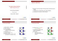
Learning Objectives
The DCT domain and JPEG
CSM25 Secure Information Hiding
Dr Hans Georg Schaathun
University of Surrey
Be able to work with and JPEG images and other representations
in the transform domain.
Understand what happens during JPEG compression, and its
potential consequence to watermarking and steganography.
Be able to apply simple LSB embedding in the JPEG domain.
Spring 2009 – Week 3
Dr Hans Georg Schaathun The DCT domain and JPEG Spring 2009 – Week 3 1 / 47
Dr Hans Georg Schaathun The DCT domain and JPEG Spring 2009 – Week 3 2 / 47
The elements of JPEG
Overview
Overview
JPEG is not a file format
Operates on luminence and chrominance (YCbCr) (not on RGB)
Grayscale images have luminence component only.
Downsampling
Works in the DCT domain (not the spatial domain)
Quantisation
Entropy coding (lossless compression)
JPEG is a compression system
The system employs three different compression techniques
JPEG is not a file format.
Files with extension .jpeg are often JFIF or EXIF.
JFIF is traditionally the most common file format for JPEG.
EXIF is made for digital cameras and contain extra meta
information.
Dr Hans Georg Schaathun The DCT domain and JPEG Spring 2009 – Week 3 4 / 47
Dr Hans Georg Schaathun The DCT domain and JPEG Spring 2009 – Week 3 5 / 47

Reading
Overview
Image Representation
Alternatives to RGB
The RGB colour representations
Core Reading
Digital Image Processing Using MATLAB.
Chapter 6: colour images
Representation
Processing
Conversion
Chapter 8.5: JPEG compression
Chapter 4: Frequency domain processing
RGB : A colour is a vector (R, G, B)
R is amount of red light.
G is amount of green light.
B is amount of blue light.
Each pixel can be either
A colour vector (R, G, B); or
a reference to an array of colour vectors (the palette)
Each coefficient can be
∈ [0, 1]; floating point (double in matlab)
∈ {0, 1, . . . , 255}; 8-bit integer (uint8 in matlab)
∈ {0, 1, . . . , 2 16 − 1}; 16-bit integer (uint16 in matlab)
Dr Hans Georg Schaathun The DCT domain and JPEG Spring 2009 – Week 3 6 / 47
Dr Hans Georg Schaathun The DCT domain and JPEG Spring 2009 – Week 3 8 / 47
Image Representation
Alternatives to RGB
Image Representation
The blockwise DCT domain
Alternatives to RGB
Block-wise
NTSC : (Y , I, Q)
where R, G, B ∈ [0, 1].
YCbCr : (Y , Cb, Cr)
⎡ ⎤ ⎡
⎤ ⎡ ⎤
Y 0.299 0.587 0.114 R
⎣ I ⎦ = ⎣0.596 −0.274 −0.322⎦
⎣G⎦
Q 0.211 −0.523 0.312 B
⎡ ⎤ ⎡ ⎤ ⎡
⎤ ⎡ ⎤
Y 16 65.481 128.553 24.966 R
⎣Cb⎦ = ⎣128⎦ + ⎣−37.797 −74.203 112.000⎦
⎣G⎦
Cr 128 112.000 −93.786 −18.214 B
Each colour-channel (Y,Cb,Cr) considered separately
M × N matrix divided into 8 × 8 blocks
Each block is handled separately
where R, G, B ∈ [0, 1] and Y , Cb, Cr ∈ [0, 255].
Dr Hans Georg Schaathun The DCT domain and JPEG Spring 2009 – Week 3 9 / 47
Dr Hans Georg Schaathun The DCT domain and JPEG Spring 2009 – Week 3 10 / 47

Image Representation
The blockwise DCT domain
Image Representation
The blockwise DCT domain
The DCT transform
The DCT transform
Several different DCT transform.
We use the following.
T f (u, v) =
where
M−1
∑
N−1
∑
x=0 y=0
√
α(u)α(v)
f (x, y)
cos
MN
α(a) =
M = N = 8,
{
1, if a = 0,
2, otherwise.
(2x + 1)uπ
2M
cos
(2y + 1)vπ
2N
The inverse is similar
f (x, y) =
where
M−1
∑
N−1
∑
u=0 v=0
√
α(u)α(v)
T f (u, v)
cos
MN
α(a) =
M = N = 8,
{
1, if a = 0,
2, otherwise.
(2x + 1)uπ
2M
cos
(2y + 1)vπ
2N
Dr Hans Georg Schaathun The DCT domain and JPEG Spring 2009 – Week 3 11 / 47
Dr Hans Georg Schaathun The DCT domain and JPEG Spring 2009 – Week 3 12 / 47
Image Representation
The blockwise DCT domain
Image Representation
The blockwise DCT domain
Matlab
Transform image
Matlab functions
dct2 (2D DCT transform)
idct2 (Inverse)
blkproc ( X, [M N], FUN )
For instance
blkproc ( X, [8 8], @dct2 )
Use help system for details
Do not use imread for JPEG images
converts images to the spatial domain.
you don’t even know the compression parameters...
Linear combination of patterns (see
right)
DC (upper left) gives average colour
intensity
Low frequency: coarse structure
High frequency: fine details
Dr Hans Georg Schaathun The DCT domain and JPEG Spring 2009 – Week 3 13 / 47
Dr Hans Georg Schaathun The DCT domain and JPEG Spring 2009 – Week 3 14 / 47

Compression
Downsampling
Compression
Downsampling
What is sampling?
What do we save?
Fact
The human eye is more sensitive to changes in luminance than in
chrominance.
To sample is to collect measurements.
Each pixel is a sample (measuring the colour of the image).
Lower resolution means fewer samples.
Reducing resolution = downsampling
Basic M × N image: N · M samples per component (Y , Cb, Cr).
Y is more useful than Cb and Cr.
Therefore we can downsample Cb and Cr
M/2 × N/2 is common for Cb and Cr
Still use M × M for Y
Original: M × N pixels ×3 components .
Compressed:
Ratio
We just saved 50%
2 × M 2 × N 2 + M × N = 11 2 M × N
Compressed
Original
= 1 1 2 MN
3MN = 1 2 .
Dr Hans Georg Schaathun The DCT domain and JPEG Spring 2009 – Week 3 16 / 47
Dr Hans Georg Schaathun The DCT domain and JPEG Spring 2009 – Week 3 17 / 47
Compression
Downsampling
Chrominance versus Luminence
Compression
Downsampling in JPEG
Downsampling
Fact
The human eye is more sensitive to changes in luminance than in
chrominance.
Watermarking tend to embed in Y (luminence)
Embedding in Cb and Cr would more easily be destroyed by
JPEG
1 Translation to YCbCr.
2 Downsampling
3 DCT transform
Each downsampled component matrix Y , Cb, Cr is
Divided into 8 × 8 blocks
DCT transformed blockwise
An 8 × 8 block in Cb can be associated with 1,2 or 4 Y blocks
depending on downsampling.
Dr Hans Georg Schaathun The DCT domain and JPEG Spring 2009 – Week 3 18 / 47
Dr Hans Georg Schaathun The DCT domain and JPEG Spring 2009 – Week 3 19 / 47

Compression
Quantisation
Compression
Quantisation
What is quantisation?
Rounding in general
Quantisation in JPEG
Rounding numbers is quantisation.
Measuring gives continuous numbers
Whether you measure pixel luminence, or the length of
your garage.
No matter how close to points are,
there is a point in between.
However, our precision is limited.
We give lengths to the nearest unit.
Luminence is categorised into 256 intervals (8bit
integers).
Computer memory is finite,
256 different possibilites for a byte
Quantisation in the DCT domain
Each coefficient is divided by the quantisation constant.
The result is rounded to nearest integer.
Different quantisation constants for each coefficient in the block.
Dr Hans Georg Schaathun The DCT domain and JPEG Spring 2009 – Week 3 20 / 47
Dr Hans Georg Schaathun The DCT domain and JPEG Spring 2009 – Week 3 21 / 47
Example
Quantisation in JPEG
Compression
Quantisation
2
3 2
3
DCT matrix
Quantisation matrix
−415 −30 −61 27 56 −20 −2 0
16 11 10 16 24 40 51 61
4 −22 −61 10 13 −7 −9 5
12 12 14 19 26 58 60 55
−47 7 77 −25 −29 10 5 −6
14 13 16 24 40 57 69 56
−49 12 34 −15 −10 6 2 2
./
14 17 22 29 51 87 80 62
12 −7 −13 −4 −2 2 −3 3
18 22 37 56 68 109 103 77
6 −8 3 2 −6 −2 1 4 2
7 624 35 55 64 81 104 113 92
7
4 −1 0 0 −2 −1 −3 4 −15
449 64 78 87 103 121 120 1015
0 0 −1 −4 −1 0 1 2 72 92 95 98 112 100 103 99
2
3
Quantised DCT matrix
−26 −3 −6 2 2 −1 0 0
0 −2 −4 1 1 0 0 0
−3 1 5 −1 −1 0 0 0
≈
−4 1 2 −1 0 0 0 0
1 0 0 0 0 0 0 0
6 0 0 0 0 0 0 0 0
7
4 0 0 0 0 0 0 0 05
0 0 0 0 0 0 0 0
Example from Wikipedia.
Entropy Coding
Recall
Compression
Source Coding
⎡
⎤
−26 −3 −6 2 2 −1 0 0
0 −2 −4 1 1 0 0 0
−3 1 5 −1 −1 0 0 0
−4 1 2 −1 0 0 0 0
1 0 0 0 0 0 0 0
⎢ 0 0 0 0 0 0 0 0
⎥
⎣ 0 0 0 0 0 0 0 0⎦
0 0 0 0 0 0 0 0
Observe
0 is extremely common
±1 is common
Two-digit numbers are very rare
This is typical
Dr Hans Georg Schaathun The DCT domain and JPEG Spring 2009 – Week 3 22 / 47
Dr Hans Georg Schaathun The DCT domain and JPEG Spring 2009 – Week 3 23 / 47

Compression
Source Coding
Steganography in JPEG
Into the compressed domain
Entropy Coding
Before or after compression
In order to compress the data
Use few bits (short codewords) for frequent symbols
Many bits (long codewords) only for rare symbols
Usually, JPEG uses a simple Huffman code.
it can use other codes (saving space, but computionally costly)
For instance, a single short codeword to say
‘the rest of the block is zero’
pixmap
pixmap
message
LSB
embedding
JPEG
compression
JPEG
compression
message
LSB
embedding
stegoimage
stegoimage
Dr Hans Georg Schaathun The DCT domain and JPEG Spring 2009 – Week 3 24 / 47
Dr Hans Georg Schaathun The DCT domain and JPEG Spring 2009 – Week 3 26 / 47
Steganography in JPEG
Into the compressed domain
Steganography in JPEG
Into the compressed domain
Fragility of LSB
When fragility is a problem
LSB embedding is criticised for being fragile
JPEG removes insignificant information
... such as the LSB
JPEG compression after embedding (probably) ruins the message
When is this a problem?
It is a problem in robust watermarking
JPEG compression is common-place
most applications need robustness
If the purpose is steganography,
and Alice and Bob are allowed to exchange pixmaps,
then it is not a problem.
Obviously, if your steganogram is supposed to be JPEG
... Do not do LSB in the pixmap.
Dr Hans Georg Schaathun The DCT domain and JPEG Spring 2009 – Week 3 27 / 47
Dr Hans Georg Schaathun The DCT domain and JPEG Spring 2009 – Week 3 28 / 47

Steganography in JPEG
Into the compressed domain
Steganography in JPEG
Into the compressed domain
Double compression
Important lessons
Common bug in existing software
Read an arbitrary image file
JPEG is decompressed on reading
... → pixmap
Embedding works on JPEG
image is compressed to produce JPEG signal
quality factor (QF) either default or supplied by user
A JPEG steganogram has now been compressed twice
different QF produces an artifact
Is there any reason for de- and recompressing?
1 Do not make unnecessary image conversions.
2 Many techniques apply to any format
LSB applies to JPEG signals
... but it is called Jsteg
3 Use a technique which fits the target (stego-) format
i.e. the format you are allowed to use on the channel.
Dr Hans Georg Schaathun The DCT domain and JPEG Spring 2009 – Week 3 29 / 47
Dr Hans Georg Schaathun The DCT domain and JPEG Spring 2009 – Week 3 30 / 47
Main development
The past at a glance
Steganography in JPEG
Into the compressed domain
The JSteg algorithm
Steganography in JPEG JSteg and OutGuess 0.1
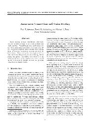
Core Reading
Hide and Seek: An Introduction to Steganography by Niels Provos and
Peter Honeyman, in IEEE Security & Privacy 2003.
1 JSteg was published
2 JSteg was broken
3 OutGuess was published
4 OutGuess was broken
5 F5 was published
6 F5 was broken
JSteg denotes a software package.
Approach: simple LSB in the DCT domain.
No different from LSB in the spatial domain
χ 2 analysis applies
Dr Hans Georg Schaathun The DCT domain and JPEG Spring 2009 – Week 3 31 / 47
Dr Hans Georg Schaathun The DCT domain and JPEG Spring 2009 – Week 3 32 / 47

Steganography in JPEG JSteg and OutGuess 0.1
Steganography in JPEG JSteg and OutGuess 0.1
Pseudocode
The JSteg algorithm
Bitflips in JSteg
Input: Image I, Message ⃗m
Output: Image J
for each bit b of ⃗m
c := next DCT coefficient from I
while c = 0 or c = 1,
c := next DCT coefficient from I
end while
c := c − c mod 2 + b
replace coefficient in I by c
end for
Cover
Stego
−5
−5
−4
−3
−4 −3
−2
−1
−2 −1
0 +1 +2 +3 +4 +5
0 +1 +2 +3 +4 +5
May ignore high and/or low frequency coefficients
Typical JPEG.
Typical JSteg.
Dr Hans Georg Schaathun The DCT domain and JPEG Spring 2009 – Week 3 33 / 47
Dr Hans Georg Schaathun The DCT domain and JPEG Spring 2009 – Week 3 34 / 47
Steganography in JPEG JSteg and OutGuess 0.1
Steganography in JPEG JSteg and OutGuess 0.1
Pros and Cons
Outguess 0.1
Why is JSteg important?
First publicly available solution.
Simple solution
What are the disadvantages?
Similar to LSB in Spatial domain.
Histogramme analysis applies
χ 2 /pairs of values applies
How can we improve JSteg?
How did we improve LSB in the Spatial Domain?
Solution
Choose random coefficients from the entire image.
Dr Hans Georg Schaathun The DCT domain and JPEG Spring 2009 – Week 3 35 / 47
Dr Hans Georg Schaathun The DCT domain and JPEG Spring 2009 – Week 3 36 / 47

Pseudocode
Outguess 0.1
Steganography in JPEG JSteg and OutGuess 0.1
Histogramme analysis
Steganalysis
Steganography in JPEG JSteg and OutGuess 0.1
Input: Image I, Message ⃗m, Key k
Output: Image J
Seed PRNG with k
for each bit b of ⃗m
c := pseudo-random DCT coefficient from I
while c = 0 or c = 1,
c := pseudo-random DCT coefficient from I
end while
c := c − c mod 2 + b
replace coefficient in I by c
end for
1 Pairs of values
Generalised χ 2 works
2 Symmetry
Embedding exchange +2 ↔ +3 and −2 ↔ −1.
The DCT histogramme is expected to be symmetric
Outguess/JSteg destroy the symmetry.
May ignore high and/or low frequency coefficients
Dr Hans Georg Schaathun The DCT domain and JPEG Spring 2009 – Week 3 37 / 47
Dr Hans Georg Schaathun The DCT domain and JPEG Spring 2009 – Week 3 38 / 47
Matlab
The JPEG toolbox
Matlab
The JPEG toolbox
JPEG Toolbox
Reading a JPEG image
JPEG Toolbox
JPEG data
» im = jpeg_read ( ’Kerckhoffs.jpg’ )
im =
image_width: 180
image_height: 247
image_components: 3
image_color_space: 2
jpeg_components: 3
jpeg_color_space: 3
comments: {}
coef_arrays: {[248x184 double] [128x96 double] [128x96 double]}
quant_tables: {[8x8 double] [8x8 double]}
ac_huff_tables: [1x2 struct]
dc_huff_tables: [1x2 struct]
optimize_coding: 0
comp_info: [1x3 struct]
progressive_mode: 0
»
Dr Hans Georg Schaathun The DCT domain and JPEG Spring 2009 – Week 3 40 / 47
» Xy = im.coef_arrays{im.comp_info(1).component_id} ;
» whos Xy
Name Size Bytes Class Attributes
Xy 248x184 365056 double
» Q = im.quant_tables{im.comp_info(1).quant_tbl_no}
Q =
»
6 4 4 6 10 16 20 24
5 5 6 8 10 23 24 22
6 5 6 10 16 23 28 22
6 7 9 12 20 35 32 25
7 9 15 22 27 44 41 31
10 14 22 26 32 42 45 37
20 26 31 35 41 48 48 40
29 37 38 39 45 40 41 40
Dr Hans Georg Schaathun The DCT domain and JPEG Spring 2009 – Week 3 41 / 47

Matlab
The JPEG toolbox
Matlab
The JPEG toolbox
w/o the toolbox
Load/Save workspace
Other toolbox functions
jpeg_read and jpeg_write are compiled functions,
Available on web page for Intel/Linux and Intel/Windows
Compilation required for other systems.
If you have trouble with the toolbox, it is possible to load/save files
as Matlab workspaces.
» load ’image.mat’
» whos
Name Size Bytes Class Attributes
im 1x1 575836 struct
If you want to write your own (de)compressor, the following
functions are useful.
bdct, ibdct, quantize, dequantize
There is one mat-file for each image on the web page
Dr Hans Georg Schaathun The DCT domain and JPEG Spring 2009 – Week 3 42 / 47
Dr Hans Georg Schaathun The DCT domain and JPEG Spring 2009 – Week 3 43 / 47
Matlab
Randomness
Matlab
Randomness
Pseudo-random number generators
Random locations
A pseudo-random number generator (PRNG)
finite state machine
starting state given by user input – the seed
each transition outputs a number
observing a sequence of number,
it is computationally infeasible to predict the next number
looks random
It is deterministic
if sender and receiver share the seed (a key)
they can generate the same sequence
Many ways to do it
but some makes it hard to avoid using the same pixel twice
A simple approach
1 randomly permute the pixels
2 embed in the first pixels in the permuted sequence
3 reverse the permutation
If the sender and receiver use the same PRNG seed,
they get the same pseudo-random permutation
Dr Hans Georg Schaathun The DCT domain and JPEG Spring 2009 – Week 3 44 / 47
Dr Hans Georg Schaathun The DCT domain and JPEG Spring 2009 – Week 3 45 / 47

Matlab
Randomness
Matlab
Masking
Matlab functions
Masking
Boolean matrix as index
Many functions using a PRNG
rand, randperm, randn
And one dedicated for performing random permutations
new = randintrlv ( old, seed )
the seed is given directly when the permutation is used
reverse: old = randdeintrlv ( new, seed )
new/old should be a 1D vector
serialise the image into a vector (im(:))
before randintrlv
reshape ( vector, [ N, M ] ) to recover the 2D image
after randdeintrlv
Matlab allows Boolean (logical) matrices as indices
Say A is an n × m matrix
B = logical(ones(n,m))
B(1,1) = 0
A(B) will be all elements of A except (1, 1)
repmat(B,m,n) replicates B to form a larger matrix
m times the heigh
n times the width
How do you extract the AC coefficients in a JPEG image?
Make an 8 × 8 mask of ones
Set the DC entry to 0, e.g. (1, 1)
Replicate the mask using repmat
Dr Hans Georg Schaathun The DCT domain and JPEG Spring 2009 – Week 3 46 / 47
Dr Hans Georg Schaathun The DCT domain and JPEG Spring 2009 – Week 3 47 / 47