Investigating the Cloud Computing Business Framework (CCBF ...
Investigating the Cloud Computing Business Framework (CCBF ...
Investigating the Cloud Computing Business Framework (CCBF ...

You also want an ePaper? Increase the reach of your titles
YUMPU automatically turns print PDFs into web optimized ePapers that Google loves.
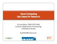
<strong>Investigating</strong> <strong>the</strong> <strong>Cloud</strong> <strong>Computing</strong><br />
<strong>Business</strong> <strong>Framework</strong> (<strong>CCBF</strong>) -<br />
Modelling and Benchmarking of<br />
Financial Assets and job<br />
submissions in <strong>Cloud</strong>s<br />
Victor Chang and Gary Wills, University of Southampton, UK.<br />
David De Roure, University of Oxford and University of<br />
Southampton, UK.<br />
Clinton Chee, Commonwealth Bank of Australia, Sydney.<br />
15 September 2010, Cardiff
Overview<br />
• Literature reviews. Finance application<br />
portability for this demo.<br />
• Introduce <strong>CCBF</strong> - Financial <strong>Cloud</strong> <strong>Framework</strong><br />
(FCF) and Middleware <strong>Framework</strong>.<br />
• Explain Monte Carlo Methods (MCM) and Black<br />
Scholes Models (BSM).<br />
• Codes and experiments used in different clouds.<br />
• Discussions<br />
• Conclusion with Q & A.
Technical and <strong>Business</strong> Challenges<br />
Literature reviews, technical and business challenges are identified.<br />
Technical:<br />
• Vendors’ lock-in;<br />
• Interoperability;<br />
• Security;<br />
<strong>Business</strong>:<br />
• Little linkage between quantitative and qualitative cloud business<br />
frameworks working in <strong>the</strong> same domain. Most are ei<strong>the</strong>r quantitative<br />
or qualitative.<br />
• Not many structured frameworks to measure cloud business<br />
performance. Some are in preliminary stage.<br />
• Application portability from desktops to clouds, and later on between<br />
clouds offered by different vendors, is challenging.<br />
Why bo<strong>the</strong>r portability<br />
• Need not rewrite API or recode/redesign software. Save $ & time.<br />
• Recessions triggered by finance – <strong>the</strong>y cannot longer just hold data<br />
without sharing. <strong>Cloud</strong>s offer a good platform for joint analysis.
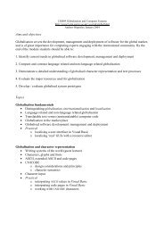
Some issues related to Finance<br />
• Global recessions triggered by Finance is an interdisciplinary<br />
research challenge.<br />
• Not many/few Universities are dealing with Financial cloud.<br />
• Many financial modelling calculations are on desktops.<br />
• Grid/HPC approaches: tend to deal with large scale calculations, &<br />
are less flexible to deal with fast-paced finance challenges/issues.<br />
• Finance applications use VBA, VB and Visual C++ etc, and need not<br />
use HPC benchmark or HPC languages (o<strong>the</strong>r than C++), at least<br />
not all <strong>the</strong> times.<br />
• Some firms/banks just use Excel or desktop software. Despite <strong>the</strong>re<br />
are interests in clouds, <strong>the</strong>y don’t know how to do, or have<br />
impression it costs a lot of money/effort, or just outsource. Portability<br />
for <strong>the</strong>m is a business challenge.
<strong>Cloud</strong> <strong>Computing</strong> <strong>Business</strong> <strong>Framework</strong><br />
(<strong>CCBF</strong>): Our motivation and approaches<br />
• <strong>CCBF</strong>: contains 4 frameworks. Use strategic/top-down<br />
approaches to identify problems, and use bottom-up<br />
methods to verify (experiments, modelling, simulations,<br />
visualisation etc).<br />
• <strong>CCBF</strong> includes Middleware <strong>Framework</strong> (MF) & Financial<br />
<strong>Cloud</strong> <strong>Framework</strong> (FCF). MF deals with IaaS and PaaS<br />
portability. FCF deals with SaaS portability issue.<br />
• This paper focuses more on FCF, and presents existing<br />
problems in Finance; and our proposal, analysis,<br />
experimental results, discussions and recommendation.
Monte Carlo Methods (MCM) Part 1<br />
• MCM, Capital Asset Models and Binomial Model etc are studied. Most<br />
commonly used method for finance is MCM, that’s why it’s chosen. We use<br />
MCM for pricing calculation.<br />
• MATLAB is used due to its ease of use with relatively good speed. While <strong>the</strong><br />
volatility is known and provided, prices for buy and sale can be calculated.<br />
• The following code demonstrates calculation of prices. Call prices are for buy<br />
and put prices are for sale.<br />
> fareastmc<br />
[LowerLimit MCPrice UpperLimit]<br />
Call Prices: [4.196694 4.248468 4.300242]<br />
Put Prices: [7.610519 7.666090 7.721662]<br />
• MCM application is in <strong>the</strong> form of a VBA Excel program to calculate <strong>the</strong> best<br />
call and put prices. For example, Spot Price = 100; Strike Price = 105;<br />
Volatility = 0.1; Risk free rate = 0.05, Option Maturity = 1; Time steps = 10 and<br />
Number of simulations are 10000. The VBA Excel program will calculate <strong>the</strong><br />
best call price as 4.009, and best put price as 3.903.
Monte Carlo Methods (MCM) Part 2<br />
Key advantages:<br />
•A large number of simulations can be calculated in one go; eg 100,000.<br />
•MCM have been widely used and proven in many cases. Calculations are close<br />
to reality if key data such as volatility, risk free rate etc are known.<br />
•Speed, accuracy and portability can be demonstrated. See core part of a code.<br />
• MCM are used in Operational Risk and models are used to simulate <strong>the</strong><br />
operational risks in Commonwealth Bank, Australia (CBA).<br />
• MCM simulations are written in Fortran and C#. Such simulations may<br />
take several hours or over a day. Results are useful for banks.<br />
• For our work, we use Variance-Gamma (VG) Processes (a specific<br />
technique in MCM) to be used for experiments and benchmark in <strong>the</strong> clouds.<br />
• VG processes are suitable in reducing errors apart from fast calculations.<br />
Details for VG processes and its experimental results in Public and Private<br />
<strong>Cloud</strong>s are in slide 8-10.
Black Scholes Model (BSM)<br />
• Methods such as Fourier series, stochastic volatility &BSM are used<br />
for volatility. As a main stream option, BSM is selected for risk<br />
analysis.<br />
• BSM has finite difference equations to approximate derivatives. We<br />
write MATLAB code to calculate call price and risk analysis based<br />
on BSM, and contain key values such as<br />
• strike price: <strong>the</strong> price targeted for sale.<br />
• upper boundary: <strong>the</strong> highest possible range a price or risk can<br />
reach.<br />
• risk free rate: interest investors would expect from an absolutely<br />
risk-free investment over a period of time.<br />
• maturity: <strong>the</strong> loan is due to be repaid on a fixed date.<br />
• volatility: used to quantify <strong>the</strong> risk of assets.<br />
• dividend yield: <strong>the</strong> return on investment for an asset.<br />
• asset steps: a specific BSM method called explicit time steps. The<br />
more steps, <strong>the</strong> more accurate <strong>the</strong> analysis.<br />
• This allows us to calculate and track call prices if variations for<br />
maturity, risk free rate and volatility change. Easy to track volatility<br />
for risk analysis if o<strong>the</strong>r variables are changed.
Experiments in <strong>Cloud</strong>s Part 1<br />
• 1 Desktop, 1 Public <strong>Cloud</strong> (Amazon) and 2 Private <strong>Cloud</strong>s (hardware spec –<br />
refer to our paper) are used for portability – run <strong>the</strong> same program, run<br />
simulation/calculation and record down time taken. Pictures of private<br />
clouds. We are interested in SaaS (finance application) running on private<br />
clouds.
Experiments in <strong>Cloud</strong>s Part 2<br />
• VG Processes (a technique in MCM) is used.<br />
• MATLAB 2007 and Octave 3.2.4 are used to run 5,000, 10,000 and<br />
15,000 simulations on <strong>Cloud</strong>s. Timing is important to run a large No<br />
of simulations!<br />
• MATLAB – runs nearly 5 times faster than Octave, but more<br />
expensive and difficult to set up. Table below summarises <strong>the</strong> timing<br />
benchmark result while running <strong>the</strong> modelling of assets (MoA) code.<br />
Number of simulations and time<br />
taken (sec)<br />
5,000 10,000 15,000<br />
Desktop 11.08 11.92 12.71<br />
Public cloud (large instance) 11.95 12.30 13.15<br />
Private cloud (virtual server)<br />
Private cloud (rack server)<br />
11.31 12.13 12.90<br />
9.63 10.51 11.48
Experiments in <strong>Cloud</strong>s Part 3<br />
time taken (sec)<br />
3.5<br />
3<br />
2.5<br />
2<br />
1.5<br />
1<br />
0.5<br />
0<br />
1 2 3<br />
Desktop<br />
Private <strong>Cloud</strong> (virtual<br />
server)<br />
Private cloud (rack<br />
server)<br />
• This Figure shows <strong>the</strong> time taken<br />
for 5,000, 10,000 and 15,000<br />
simulations with MATLAB 2007<br />
on desktop and 2 private<br />
clouds. Public cloud is not<br />
available at <strong>the</strong> time for testing.<br />
Private cloud (rack server) needs<br />
<strong>the</strong> least amount of time.<br />
MCM simulations (1 unit = 5,000 simulations)<br />
time taken (sec)<br />
6<br />
5<br />
4<br />
3<br />
2<br />
1<br />
0<br />
1 2 3<br />
No of steps taken (1 unit = 500 steps)<br />
Desktop<br />
Public cloud (large<br />
instance(<br />
Private cloud (virtual<br />
server)<br />
Private cloud (rack<br />
server)<br />
• This Figure shows <strong>the</strong> time taken<br />
for running 500, 1,000 and 1,500<br />
steps in BSM application on 4<br />
different clouds and 1 desktop.<br />
Time series used in BSM can take<br />
accommodate up to 1,500<br />
simulations. Private cloud (rack<br />
server) has <strong>the</strong> best hardware<br />
configuration with <strong>the</strong> fastest<br />
network speed & significantly high<br />
bandwidth, so it runs <strong>the</strong> fastest.
Middleware <strong>Framework</strong> – GridSAM 2.3<br />
• GridSAM is widely used in <strong>the</strong> UK community and is very easy to modify <strong>the</strong><br />
Job Submission Description Language (JSDL) for job submission. The<br />
GridSAM 2.3 contains bespoke application that allows multiple submissions for<br />
around 20,000 jobs submitted at each instance.<br />
• A Java program, Primes, is written to list prime numbers, and is able to submit<br />
jobs to Private and Public <strong>Cloud</strong>s. For example: Two JSDL files, primes-<br />
0to10000.jsdl and prime-10001to20000.jsdl are written to send 20,000 jobs,<br />
and a primes_file.pl is modified to lists prime numbers between 0 and 20,000.<br />
7.5<br />
7<br />
6.5<br />
Time taken (sec)<br />
6<br />
5.5<br />
5<br />
Public cloud<br />
Private cloud<br />
(virtual server)<br />
Private cloud<br />
(rack server)<br />
• Job submission and its<br />
status check is used to<br />
record time taken.<br />
4.5<br />
4<br />
1 2 3 4<br />
No of jobs submitted (1 unit =5,000 jobs)
Three implications for Banking<br />
• Three implications: Security; Financial Regulations and<br />
Portability.<br />
• Security: Evolving challenges in location of clouds and data privacy.<br />
Mechanisms such as X509 vs. single sign-on are discussed.<br />
• Regulations: Tighter risk management controls. <strong>Cloud</strong> computation<br />
and resources help financial institutions in running more analytical<br />
simulations to calculate risks to <strong>the</strong> client organisations.<br />
• Portability: letting clients to install <strong>the</strong>ir own libraries. Users who run<br />
MATLAB only need to install <strong>the</strong> MATLAB Runtime to run MATLAB<br />
executable on <strong>Cloud</strong>s. For financial simulations written in Fortran or<br />
C++, users may need Math libraries to be installed in <strong>the</strong> <strong>Cloud</strong>s.<br />
• <strong>Cloud</strong>s must facilitate an easy way to install and configure user<br />
required libraries, without <strong>the</strong> need to write additional APIs like several<br />
practices do.
Conclusion and Future Work<br />
• MCM, BSM and GridSAM are used to demonstrate how<br />
portability, speed, accuracy and reliability can be achieved<br />
while moving financial applications from desktops to clouds.<br />
This well fits-in an objective in <strong>the</strong> <strong>CCBF</strong> to allow portability<br />
on top of, secure, fast, accurate and reliable clouds for IaaS,<br />
PaaS and SaaS.<br />
• Our research is not intended to test pure computing<br />
performance of <strong>Cloud</strong> <strong>Computing</strong>. The intention is to port and<br />
test financial applications to run on <strong>the</strong> <strong>Cloud</strong>. It is not yet<br />
critical to use Dongarra's netlib functions for benchmark, but<br />
<strong>the</strong>re are plans to use HPC languages such as (Visual) C++<br />
& test on 6-core processing private clouds for next stage.<br />
• We have Health <strong>Cloud</strong> Storage <strong>Framework</strong> (HCSF) that can<br />
demonstrate portability in details. We hope to streng<strong>the</strong>n our<br />
results and extents of collaboration (such as financial services<br />
and non-UK governments).
An example in Private Clod: 6-core & 4 terabytes<br />
• Upgradable to 16 GB DDR3, 8-12 TB per server. Cost effective with high<br />
performance capabilities.<br />
• Better performances in MCM and BSM financial applications.
Collaboration and Questions<br />
O<strong>the</strong>r collaborators: 2 anonymous government department<br />
branches, 2 anonymous investment banks and 3<br />
anonymous small/medium enterprises.<br />
Thank you!
Appendix: An example in Monte Carlo Methods (MCM)<br />
%%%%% Input parameters<br />
%%%%%%%%<br />
S=100; %spot price<br />
K=105; %strike<br />
T=1; %maturity<br />
r=0.05; %interest rate<br />
sigma=0.25; %volatility<br />
NSimulations=100000; %no of<br />
monte carlo simulations<br />
NSteps=100; %no of time steps<br />
%%%%%%%%%%%%%%%%%<br />
%%%%%%%%%%%%%%<br />
dt=T/(NSteps-1);<br />
vsqrdt=sigma*dt^0.5;<br />
drift=(r-(sigma^2)/2)*dt;<br />
x=randn(NSimulations,NSteps);<br />
Smat=zeros(NSimulations,NStep<br />
s);<br />
Smat(:,1)=S;<br />
for i=2:NSteps,<br />
Smat(:,i)=Smat(:,i-<br />
1).*exp(drift+vsqrdt*x(:,i));<br />
end<br />
%************* calculate call price ***********<br />
callpayoffvec=max(AverageSVec-K,0);<br />
mccallprice=exp(-r*T)*mean(callpayoffvec);<br />
std_dev_call=(var(callpayoffvec))^0.5;<br />
%calculate bounds of expected value assuming 95%<br />
confidence level<br />
mclimit_call=1.96*std_dev_call/NSimulations^0.5;<br />
call_lowerlimit=mccallprice-mclimit_call;<br />
call_upperlimit=mccallprice+mclimit_call;<br />
printf("Call Prices : [%f %f<br />
%f]\n",call_lowerlimit,mccallprice,call_upperlimit);<br />
%************* calculate put price ***********<br />
putpayoffvec=max(K-AverageSVec,0);<br />
mcputprice=exp(-r*T)*mean(putpayoffvec);<br />
std_dev_put=(var(putpayoffvec))^0.5;<br />
%calculate bounds of expected value assuming 95%<br />
confidence level<br />
mclimit_put=1.96*std_dev_put/NSimulations^0.5;<br />
put_lowerlimit=mcputprice-mclimit_put;<br />
put_upperlimit=mcputprice+mclimit_put;<br />
printf("Put Prices : [%f %f<br />
%f]\n",put_lowerlimit,mcputprice,put_upperlimit);
Appendix: An example in Black Scholes Model (BSM)<br />
%----------- Enter input Parameters -----------------------<br />
S=100; %Spot price<br />
K=100; %Strike<br />
UB=115; %upper boundary<br />
r=0.15; %risk free rate<br />
T=.5; %maturity<br />
sigma=0.2; %volatility<br />
D=0.05; %dividend yield<br />
assetsteps=150; %Explicit scheme time steps<br />
%----------------------------------------------------<br />
dt=1/(sigma*assetsteps)^2;<br />
timesteps=ceil(T/dt)+1;<br />
Su=UB;<br />
ds=Su/assetsteps;<br />
dt=T/timesteps;<br />
for k=1:timesteps,<br />
V(2:assetsteps,k+1)=Ai.*V(1:assetsteps-<br />
1,k)+(1+Bi).*V(2:assetsteps,k)+Ci.*V(3:assetsteps<br />
+1,k);<br />
%Apply lower boundary condition<br />
V(1,k+1)=0;<br />
%apply upper boundary condition<br />
V(assetsteps+1,k+1)=0;<br />
end<br />
V2=fliplr(V);<br />
OptionPriceVec=V2(:,1);<br />
option_price=interp1(Svec,OptionPriceVec,S)<br />
V=zeros(assetsteps+1,timesteps+1);<br />
Svec=0:ds:Su;<br />
Svec=Svec';<br />
V(:,1)=max((Svec-K).*(Svec