Methods of Vanishing Viscosity for Nonlinear ... - ACMAC
Methods of Vanishing Viscosity for Nonlinear ... - ACMAC
Methods of Vanishing Viscosity for Nonlinear ... - ACMAC

Create successful ePaper yourself
Turn your PDF publications into a flip-book with our unique Google optimized e-Paper software.
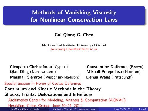
<strong>Methods</strong> <strong>of</strong> <strong>Vanishing</strong> <strong>Viscosity</strong><br />
<strong>for</strong> <strong>Nonlinear</strong> Conservation Laws<br />
Gui-Qiang G. Chen<br />
Mathematical Institute, University <strong>of</strong> Ox<strong>for</strong>d<br />
Gui-Qiang.Chen@maths.ox.ac.uk<br />
Cleopatra Christ<strong>of</strong>orou (Cyprus)<br />
Qian Ding (Northwestern)<br />
Marshall Slemrod (Wisconsin-Madison)<br />
Constantine Dafermos (Brown)<br />
Mikhail Perepelitsa (Houston)<br />
Dehua Wang (Pittsburgh)<br />
Special Session in Honor <strong>of</strong> Costas Dafermos<br />
Continuum and Kinetic <strong>Methods</strong> in the Theory<br />
Shocks, Fronts, Dislocations and Interfaces<br />
Archimedes Center <strong>for</strong> Modeling, Analysis & Computation (<strong>ACMAC</strong>)<br />
Heraklion, Crete, Greece, June 20–24, 2011<br />
Gui-Qiang Chen (Ox<strong>for</strong>d) <strong>Vanishing</strong> <strong>Viscosity</strong>/Conservation Laws June 20–24, 2011 1 / 40
<strong>Methods</strong> <strong>of</strong> <strong>Vanishing</strong> <strong>Viscosity</strong><br />
Hyperbolic Conservation Laws:<br />
∂ t U(t, x) + ∂ x F (U(t, x)) = 0,<br />
U(t, x) ∈ R N<br />
F : R N → R N <strong>Nonlinear</strong>: Eigenvalues <strong>of</strong> ∇ U F (U) are real<br />
∂ t U(t, x) + ∂ x F{U(t, x), U (t) (·, x)} = 0<br />
U (t) (τ, x) := U(t − τ, x)–the past history <strong>of</strong> U and x r.t. t<br />
Approaches: Honor Physical or Design Artificial N × N matrix function:<br />
D : R N → M N×N , D(U) ≥ 0<br />
∂ t U ε + ∂ x F (U ε ) =ε∂ x (D(U ε )∂ x U ε )<br />
admits a global solution U ε (t, x) <strong>for</strong> each fixed ε > 0;<br />
U ε (t, x) → U(t, x) topology ?? U(t, x) an entropy solution??<br />
Gui-Qiang Chen (Ox<strong>for</strong>d) <strong>Vanishing</strong> <strong>Viscosity</strong>/Conservation Laws June 20–24, 2011 2 / 40
<strong>Methods</strong> <strong>of</strong> <strong>Vanishing</strong> <strong>Viscosity</strong><br />
Hyperbolic Conservation Laws:<br />
∂ t U(t, x) + ∂ x F (U(t, x)) = 0,<br />
U(t, x) ∈ R N<br />
F : R N → R N <strong>Nonlinear</strong>: Eigenvalues <strong>of</strong> ∇ U F (U) are real<br />
∂ t U(t, x) + ∂ x F{U(t, x), U (t) (·, x)} = 0<br />
U (t) (τ, x) := U(t − τ, x)–the past history <strong>of</strong> U and x r.t. t<br />
Approaches: Honor Physical or Design Artificial N × N matrix function:<br />
D : R N → M N×N , D(U) ≥ 0<br />
∂ t U ε + ∂ x F (U ε ) =ε∂ x (D(U ε )∂ x U ε )<br />
admits a global solution U ε (t, x) <strong>for</strong> each fixed ε > 0;<br />
U ε (t, x) → U(t, x) topology ?? U(t, x) an entropy solution??<br />
Stokes (1848), Rayleigh (1910), Taylor (1910), Weyl (1949), · · ·<br />
Theory: Entropy Conditions, Nonuniqueness, Existence, Solution Behavior, · · ·<br />
Numerical <strong>Methods</strong>/Applications: Shock Capturing, Upwind, Kinetic, · · ·<br />
Challenges: Singular limits, · · · =⇒ New Math Ideas/<strong>Methods</strong> · · ·<br />
*Analogously <strong>for</strong> Multidimensional Setting<br />
Gui-Qiang Chen (Ox<strong>for</strong>d) <strong>Vanishing</strong> <strong>Viscosity</strong>/Conservation Laws June 20–24, 2011 2 / 40
Scalar Conservation Laws: BV -Estimates<br />
∂ t u ε + ∂ x f (u ε ) = ε∂ xx u ε<br />
Estimates: There exists C independent <strong>of</strong> ε such that<br />
Maximum Principle:<br />
BV Estimates:<br />
‖u ε ‖ L ∞ ≤ C<br />
Hopf, Oleinik, Lax, Volpert, Kruzhkov, · · ·<br />
Volpert’s Method:<br />
‖∂ x u ε ‖ L 1 + ‖∂ t u ε ‖ L 1 ≤ C<br />
∂ t (|∂ x u ε |) + ∂ x (f ′ (u ε )|∂ x u ε |) ≤ ε∂ xx (|∂ x u ε |),<br />
∂ t (|∂ t u ε |) + ∂ x (f ′ (u ε )|∂ t u ε |) ≤ ε∂ xx (|∂ t u ε |).<br />
BV-Compactness Theorem =⇒ Strong Convergence <strong>of</strong> u ε (t, x)<br />
Similar arguments to obtain <strong>for</strong> the L 1 –Equicontinuity directly<br />
A corollary <strong>of</strong> the L 1 -stability and the comparison principle via<br />
Kruzhkov’s Method<br />
∂ t u ε + ∇ x · f(u ε ) = ε∆ x u ε<br />
Gui-Qiang Chen (Ox<strong>for</strong>d) <strong>Vanishing</strong> <strong>Viscosity</strong>/Conservation Laws June 20–24, 2011 3 / 40
Nonlocal Scalar Conservation Laws: BV -Estimates<br />
∂ t u + ∂ x<br />
(<br />
f (u) +<br />
∫ t<br />
0 k δ(t − τ)f (u(τ))dτ) = 0<br />
Memory kernel: κ δ (t) ⇀ (α − 1) δ(t) when δ → 0<br />
Artificial <strong>Viscosity</strong> Method (C-Christ<strong>of</strong>orou 2007):<br />
∂ t u ε + ∂ x f (u ε ) + ∫ t<br />
0 k δ(t − τ)f (u ε (τ)) x dτ<br />
= ε∂ xx (u ε + ∫ t<br />
k 0 δ(t − τ)u ε (τ)dτ)<br />
Idea: Employ the resolvent kernel r δ (t) <strong>of</strong> k δ (t): r δ + k δ ∗ r δ = −k δ<br />
(MacCamy 1977, Dafermos 1988, Nohel-Rogers-Tzavaras 1988)<br />
=⇒ ∂ t u ε + ∂ x f (u ε ) + r δ (0)u ε = r δ (t)u 0 − ∫ t<br />
r ′ 0 δ (t − τ)uε (τ) + ε∂ xx u ε<br />
Estimates: There exists C independent <strong>of</strong> ε, δ such that<br />
BV ∩ L ∞ Estimates:<br />
‖u ε,δ ‖ L ∞ + ‖∂ x u ε,δ ‖ L 1 + ‖∂ t u ε,δ ‖ L 1 ≤ C<br />
BV-Compactness Theorem =⇒ Strong Convergence <strong>of</strong> u ε,δ (t, x)<br />
Existence and Stability <strong>of</strong> Entropy Solutions u δ (t, x) to hyperbolic<br />
conservation laws with memory as the limit <strong>of</strong> ε → 0<br />
When κ δ (t) ⇀ (α − 1) δ(t) as δ → 0, u δ (t, x) → u(t, x) in L 1 , a<br />
solution to the scalar conservation laws ∂ t u + α∂ x f (u) = 0<br />
Gui-Qiang Chen (Ox<strong>for</strong>d) <strong>Vanishing</strong> <strong>Viscosity</strong>/Conservation Laws June 20–24, 2011 4 / 40
Scalar Conservation Laws: Compensated Compactness<br />
∂ t u ε + ∂ x f (u ε ) = ε∂ xx u ε<br />
Estimates: There exists C independent <strong>of</strong> ε such that<br />
Maximum Principle: ‖u ε ‖ L ∞ ≤ C (or ‖u ε ‖ L p ≤ C)<br />
Dissipation Estimate: ‖ √ εux‖ ε L 2 ≤ C<br />
Energy Estimate:<br />
ε(∂ x u ε ) 2 = −∂ t ( (uε ) 2 ∫ u ε<br />
2 ) − ∂ x( wf ′ (w)dw) + ε∂ xx ( (uε ) 2<br />
2 )<br />
=⇒ For any η ∈ C 2 with entropy flux q(u) = ∫ u η ′ (w)f ′ (w)dw,<br />
∂ t η(u ε ) + ∂ x q(u ε )<br />
is compact in H −1<br />
loc<br />
Compensated Compactness =⇒ Strong Convergence <strong>of</strong> u ε (t, x)<br />
∂ t u ε + ∂ x f (u ε ) = ε∂ x (D(u ε )∂ x u ε )<br />
Tartar, Schonbek, DiPerna, Chen-Lu, Tadmor-Rascle-Bagnerini, · · ·<br />
Scalar Conservation Laws with Memory: Dafermos 1988<br />
Gui-Qiang Chen (Ox<strong>for</strong>d) <strong>Vanishing</strong> <strong>Viscosity</strong>/Conservation Laws June 20–24, 2011 5 / 40
Hyperbolic Systems: BV -Estimates<br />
via Glimm’s Scheme (1965)<br />
=⇒<br />
Wave Interaction Estimates<br />
BV-Estimate Techniques: Glimm Functional<br />
· · · · · ·<br />
Global Existence <strong>of</strong> Solutions in BV when the Total Variation <strong>of</strong> the<br />
Initial Data Is Small<br />
Structure <strong>of</strong> Solutions in BV<br />
Dafermos, DiPerna, · · ·<br />
Asymptotic Behavior: Decay <strong>of</strong> Periodic Solutions, · · ·<br />
Glimm-Lax, Dafermos, DiPerna, Liu, · · ·<br />
· · · · · ·<br />
Gui-Qiang Chen (Ox<strong>for</strong>d) <strong>Vanishing</strong> <strong>Viscosity</strong>/Conservation Laws June 20–24, 2011 6 / 40
Hyperbolic Systems: Artificial <strong>Viscosity</strong> via BV-Estimates I<br />
∂ t U ε + ∂ x F (U ε ) = ε∂ xx U ε ,<br />
U(0, x) = U 0 (x) ∈ R N<br />
Biachini-Bressan (2005): For strictly hyperbolic systems on U in<br />
a n.b.h.d. <strong>of</strong> a compact set K ⊂ R N , there exist constants δ > 0 and<br />
C j , j = 1, 2, 3, such that, if<br />
Tot.Var.{U 0 } < δ,<br />
lim U 0(x) ∈ K,<br />
x→−∞<br />
then, ∀ε > 0, there exists a unique solution U ε (t, ·) := S ε t U 0 (·) s.t.<br />
BV Bound: Tot.Var.{S ε t U 0 } ≤ C 1 Tot.Var.{U 0 }<br />
L 1 -Stability: ‖S ε t U 0 − S ε t V 0 ‖ L 1 ≤ C 2 ‖U 0 − V 0 ‖ L 1<br />
‖S ε t U 0 − S ε s U 0 ‖ L 1 ≤ C 3 (|t − s| + | √ εt − √ εs|)<br />
=⇒ Strong Convergence and L 1 -Stability <strong>of</strong> the Limit Solution<br />
Even <strong>for</strong> non-conservative strictly hyperbolic systems<br />
The approach requires the artificial viscosity <strong>for</strong>m<br />
The total variation <strong>of</strong> the initial data is sufficiently small<br />
Gui-Qiang Chen (Ox<strong>for</strong>d) <strong>Vanishing</strong> <strong>Viscosity</strong>/Conservation Laws June 20–24, 2011 7 / 40
Hyperbolic Systems: Artificial <strong>Viscosity</strong> via BV-Estimates II<br />
Using the heat kernel to estimate the solution <strong>for</strong> t ∈ [0, τ ε ]:<br />
‖∂ x U ε (t, ·)‖ L 1 ≤ κ δ, κ indept. <strong>of</strong> ε and δ<br />
Decompose ∂ x U ε along a suitable basis <strong>of</strong> unit vectors {r 1 , · · · , r N }:<br />
∂ x U ε = ∑ v ε<br />
i r i<br />
(Sum <strong>of</strong> gradients <strong>of</strong> viscous travelling waves)<br />
Obtain a system <strong>of</strong> N equations <strong>for</strong> these scalar components:<br />
∂ t v ε<br />
i<br />
+ ∂ x (˜λ i v ε<br />
i )−ε∂ xx v ε<br />
i = φ ε i , i = 1, · · · , N.<br />
Then, as the scalar case, we obtain that, <strong>for</strong> all t ≥ τ ε ,<br />
∫ ∞ ∫<br />
‖vi ε (t, ·)‖ L 1 ≤ ‖vi ε (τ ε , ·)‖ L 1 + |φ ε i (t, x)|dxdt.<br />
Construct the basis {r 1 , · · · , r N } in a clever way so that, <strong>for</strong> t ≥ τ ε ,<br />
∫ ∞ ∫<br />
|φ ε i (t, x)|dxdt ≤ C, C > 0 independent <strong>of</strong> ε > 0.<br />
τ ε<br />
=⇒ Tot. Var.{U ε (t, ·)} = ‖U ε x (t, ·)‖ L 1 ≤ ∑ i<br />
τ ε<br />
‖v ε<br />
i (t, ·)‖ L 1 ≤ C<br />
Gui-Qiang Chen (Ox<strong>for</strong>d) <strong>Vanishing</strong> <strong>Viscosity</strong>/Conservation Laws June 20–24, 2011 8 / 40
Hyperbolic Systems: <strong>Vanishing</strong> <strong>Viscosity</strong> via BV-Estimates<br />
Further Problem: BV Estimates and Convergence <strong>of</strong> vanishing<br />
viscosity approximation <strong>of</strong> the general <strong>for</strong>m:<br />
∂ t U ε + ∂ x F (U ε ) = ε∂ x (D(U ε )∂ x U ε )<br />
<strong>for</strong> general viscosity matrices D(U).<br />
Physical <strong>Viscosity</strong>: Navier-Stokes <strong>Viscosity</strong> Matrices?<br />
Navier-Stokes Equations =⇒Euler Equations??<br />
Gui-Qiang Chen (Ox<strong>for</strong>d) <strong>Vanishing</strong> <strong>Viscosity</strong>/Conservation Laws June 20–24, 2011 9 / 40
Artificial <strong>Viscosity</strong> via Compensated Compactness<br />
∂ t U ε + ∂ x F (U ε ) = ε∂ xx U ε<br />
Assume: The system has a strictly convex entropy function η ∗ (U).<br />
Estimates: There exists C independent <strong>of</strong> ε such that<br />
Invariant Regions: ‖U ε ‖ L ∞ ≤ C (or ‖U ε ‖ L p ≤ C)<br />
Dissipation Estimate: ‖ √ ε∂ x U ε ‖ L 2 ≤ C<br />
Energy Estimate:<br />
ε(∂ x U ε ) ⊤ ∇ 2 η ∗ (U ε )∂ x U ε = −∂ t η ∗ (U ε ) − ∂ x q ∗ (U ε ) + ε∂ xx η ∗ (U ε )<br />
=⇒ For any η ∈ C 2 with entropy flux q (i.e., ∇q(U) = ∇η(U)∇F (U) ),<br />
∂ t η(U ε ) + ∂ x q(U ε )<br />
is compact in H −1<br />
loc<br />
Compensated Compactness =⇒ Strong Convergence <strong>of</strong> U ε (t, x)<br />
∂ t U ε + ∂ x F (U ε ) = ε∂ x (D(U ε )∂ x U ε ) <strong>for</strong> ∇ 2 η ∗ (U)D(U) ≥ c 0 > 0.<br />
Large Initial Data, · · ·<br />
Gui-Qiang Chen (Ox<strong>for</strong>d) <strong>Vanishing</strong> <strong>Viscosity</strong>/Conservation Laws June 20–24, 2011 10 / 40
Compactness: Young Measure and Commutation Identity<br />
Div-Curl Lemma [Tartar (1979), Murat (1978)]<br />
Young Measure Rep. [Tartar (1979), Ball (1989), Alberti-Müller (2001)]<br />
=⇒<br />
〈ν(λ), η1 (λ)q 2 (λ) − q 1 (λ)η 2 (λ)〉<br />
= 〈ν(λ), η 1 (λ)〉〈ν(λ), q 2 (λ)〉 − 〈ν(λ), q 1 (λ)〉〈ν(λ), η 2 (λ)〉<br />
<strong>for</strong> any entropy-entropy flux pairs (η j , q j ), j = 1, 2, where ν = ν t,x (λ) is the<br />
associated Young measure (probability measure) <strong>for</strong> the sequence U ε (t, x).<br />
Issue: Is ν a Dirac measure? =⇒ Compactness <strong>of</strong> U ε (t, x) in L 1<br />
Remarks:<br />
The viscosity matrix ∇ 2 η ∗ (U)D(U) > 0 =⇒ Dissipation Estimate<br />
2 × 2 Strict Hyperbolicity: =⇒ Rich Entropy-Entropy Flux Pairs<br />
DiPerna, Dafermos, Serre, Morawetz, Perthame-Tzavaras, Chen-Li, · · · · · ·<br />
Gui-Qiang Chen (Ox<strong>for</strong>d) <strong>Vanishing</strong> <strong>Viscosity</strong>/Conservation Laws June 20–24, 2011 11 / 40
Further Challenges<br />
Nonstrictly Hyperbolic Systems<br />
Initial Data <strong>of</strong> Large Oscillation without Bounded Variation<br />
<strong>Viscosity</strong> Matrix with ∇ 2 η ∗ (U)D(U) ≥ 0 but Not Positive Definite ??<br />
No L ∞ -Uni<strong>for</strong>m Bound: Only Energy Bounds<br />
· · · · · ·<br />
Important Problems:<br />
The Compressible Navier-Stokes Equations<br />
=⇒ the Compressible Euler Equations<br />
Global Spherically Symmetric Solutions to the Compressible Euler<br />
Equations<br />
Global Solutions to the Compressible Euler Equations with Random<br />
Forcing Terms<br />
Global Solutions to Nonlocal Conservation Laws with Memory<br />
· · · · · ·<br />
Gui-Qiang Chen (Ox<strong>for</strong>d) <strong>Vanishing</strong> <strong>Viscosity</strong>/Conservation Laws June 20–24, 2011 12 / 40
Navier-Stokes Equations: Inviscid Limit<br />
with the initial conditions:<br />
ρ(0, x) = ρ 0 (x), u(0, x) = u 0 (x),<br />
{<br />
ρt + (ρu) x = 0,<br />
(ρu) t + (ρu 2 + p) x = εu xx ,<br />
lim (ρ 0(x), u 0 (x)) = (ρ ± , u ± ),<br />
x→±∞<br />
(ρ ± , u ± ) are constant end-states with ρ ± > 0<br />
The viscosity coefficient ε ∈ (0, ε 0 ] <strong>for</strong> some fixed ε 0<br />
ρ – Density, u – Velocity <strong>of</strong> Fluid when ρ > 0<br />
p = p(ρ) = ρ 2 e ′ (ρ) – Pressure with internal energy e(ρ)<br />
For a polytropic perfect gas, p(ρ) = κρ γ , e(ρ) = κ<br />
γ−1 ργ−1 , γ > 1<br />
Existence <strong>of</strong> C 2 solutions (ρ ε , u ε )(t, x) <strong>for</strong> Large Data:<br />
Ya Kanel 1968, H<strong>of</strong>f 1998<br />
Problem: Inviscid Limit <strong>of</strong> (ρ ε , u ε )(t, x) when ε → 0??<br />
Gilberg (1951), H<strong>of</strong>f-Liu (1989), Gùes-Métivier-Williams-Zumbrun (2006), · · · · · ·<br />
Gui-Qiang Chen (Ox<strong>for</strong>d) <strong>Vanishing</strong> <strong>Viscosity</strong>/Conservation Laws June 20–24, 2011 13 / 40
Limit System: Isentropic Euler Equations ??<br />
{<br />
∂t ρ + ∂ x m = 0, (m = ρu)<br />
∂ t m + ∂ x ( m2<br />
ρ + p(ρ)) = 0<br />
Strict hyperbolicity: Fails when ρ → 0 (vacuum)<br />
Entropy Pair (η, q): ∇q(U) = ∇η(U)∇F (U)<br />
Convex Entropy: ∇ 2 η(U) > 0 Weak Entropy: η(ρ, ρu)| ρ=0 = 0<br />
Weak entropy pairs are represented as<br />
∫<br />
∫<br />
η ψ (ρ, ρu) = χ(s)ψ(s) ds, q ψ (ρ, ρu) = (θs + (1 − θ)u)χ(s)ψ(s) ds<br />
R<br />
R<br />
by C 2 test functions ψ(s), where χ(s) is the weak entropy kernel:<br />
χ(s) := [ρ 2θ − (u − s) 2] λ<br />
+ , θ = γ − 1 , λ = 3 − γ<br />
2 2(γ − 1) .<br />
Physical Convex Entropy: Mechanical energy-energy flux pair (η ∗ , q ∗ ):<br />
η ∗ (ρ, m) = 1 m 2<br />
2<br />
ρ + ρe(ρ), q ∗(ρ, m) = 1 2<br />
m 3<br />
ρ 2 + m(e(ρ) + p ρ )<br />
Gui-Qiang Chen (Ox<strong>for</strong>d) <strong>Vanishing</strong> <strong>Viscosity</strong>/Conservation Laws June 20–24, 2011 14 / 40
<strong>Vanishing</strong> Artificial/Numerical <strong>Viscosity</strong> <strong>Methods</strong> I<br />
{<br />
∂t ρ + ∂ x m = ε∂ 2<br />
Artificial <strong>Viscosity</strong>:<br />
xρ,<br />
∂ t m + ∂ x ( m2 + p(ρ)) = ρ<br />
ε∂2 xm,<br />
Numerical <strong>Viscosity</strong>: Lax-Friedrichs Scheme, Godunov Scheme, · · ·<br />
Advantages: There exists C > 0, independent <strong>of</strong> ε > 0, such that<br />
Invariant Regions =⇒ L ∞ Estimate:<br />
0 ≤ ρ ε (t, x) ≤ C, 0 ≤ |m ε (t, x)| ≤ Cρ ε (t, x) a.e.<br />
√<br />
Dissipation Estimate: ε‖∂x (ρ ε , m ε )‖ L 2 ([0,T ]×R) ≤ C<br />
via the mechanical energy-entropy flux pairs (η ∗ , q ∗ ) that is<br />
strictly convex <strong>for</strong> 1 < γ ≤ 2 (and convex <strong>for</strong> γ > 2: weighted<br />
dissipation estimate).<br />
=⇒ For any C 2 weak entropy-entropy flux pair (η, q),<br />
∂ t η(ρ ε , m ε ) + ∂ x q(ρ ε , m ε )<br />
is compact in H −1<br />
loc<br />
Gui-Qiang Chen (Ox<strong>for</strong>d) <strong>Vanishing</strong> <strong>Viscosity</strong>/Conservation Laws June 20–24, 2011 15 / 40
<strong>Vanishing</strong> Artificial/Numerical <strong>Viscosity</strong> <strong>Methods</strong> II<br />
Physical Convex Entropy: Mechanical Energy-Energy Flux Pair (η ∗ , q ∗ ):<br />
η ∗ (ρ, m) = 1 m 2<br />
2 ρ + e(ρ), q ∗(ρ, m) = 1 m 3<br />
2 ρ 2 + me′ (ρ)<br />
=⇒ ∇ 2 U η ∗(U) > 0 <strong>for</strong> U = (ρ, m) when 1 < γ ≤ 2.<br />
W.O.L.G. assume that lim |x|→∞ U ε = Ū = U ± . Set<br />
Φ ∗ (U) = η ∗ (U) − η ∗ (Ū) − ∇η∗(Ū)(U − Ū) ≥ 0,<br />
Ψ ∗ (U) = q ∗ (U) − q ∗ (Ū) − ∇η∗(Ū)(F (U) − F (Ū))<br />
Multiply ∇Φ ∗ (U ε ), both sides <strong>of</strong> the system:<br />
∂ t Φ ∗ (U ε ) + ∂ x Ψ ∗ (U ε ) = ε∂ x (∇Φ ∗ (U ε )∂ x U ε ) − ε(∂ x U ε ) ⊤ ∇ 2 η ∗ (U ε )∂ x U ε .<br />
=⇒ ε ∫ T<br />
0<br />
∫ ∞<br />
−∞ (∂ xU ε ) ⊤ ∇ 2 η ∗ (U ε )∂ x U ε dxdt<br />
≤ ∫ ∞<br />
−∞ Φ ∗(U 0 (x)) dx < ∞<br />
Gui-Qiang Chen (Ox<strong>for</strong>d) <strong>Vanishing</strong> <strong>Viscosity</strong>/Conservation Laws June 20–24, 2011 16 / 40
Isentropic Euler Equations: Reduction <strong>of</strong> a Measure-Valued<br />
Solution ν t,x : supp ν Is Bounded<br />
DiPerna: γ = N+2,<br />
N<br />
Ding-Chen-Luo, Chen: γ ∈ (1, 5]<br />
3<br />
Lions-Perthame-Tadmor: γ ≥ 3<br />
Lions-Perthame-Souganidis: γ ∈ ( 5 , 3) =⇒ γ ∈ (1, 3)<br />
3<br />
Chen-LeFloch:<br />
General Pressure Laws<br />
Conclusion: If supp ν is bounded, then<br />
ν t,x = ν (ρ(t,x),m(t,x)) ,<br />
that is, (ρ ε (t, x), m ε (t, x)) → (ρ(t, x), m(t, x)) a.e. (t, x).<br />
Key Point: Employ Effectively the Weak Entropy-Entropy Flux Pairs<br />
Gui-Qiang Chen (Ox<strong>for</strong>d) <strong>Vanishing</strong> <strong>Viscosity</strong>/Conservation Laws June 20–24, 2011 17 / 40
Navier-Stokes Equations: Inviscid Limit<br />
with the initial conditions:<br />
ρ(0, x) = ρ 0 (x), u(0, x) = u 0 (x),<br />
{<br />
ρt + (ρu) x = 0,<br />
(ρu) t + (ρu 2 + p) x = εu xx ,<br />
lim (ρ 0(x), u 0 (x)) = (ρ ± , u ± ),<br />
x→±∞<br />
(ρ ± , u ± ) are constant end-states with ρ ± > 0<br />
The viscosity coefficient ε ∈ (0, ε 0 ] <strong>for</strong> some fixed ε 0<br />
ρ – Density, u – Velocity <strong>of</strong> Fluid when ρ > 0<br />
p = p(ρ) = ρ 2 e ′ (ρ) – Pressure with internal energy e(ρ)<br />
For a polytropic perfect gas, p(ρ) = κρ γ , e(ρ) = κ<br />
γ−1 ργ−1 , γ > 1<br />
Existence <strong>of</strong> C 2 solutions (ρ ε , u ε )(t, x) <strong>for</strong> Large Data:<br />
Ya Kanel 1968, H<strong>of</strong>f 1998<br />
Problem: <strong>Vanishing</strong> <strong>Viscosity</strong> Limit <strong>of</strong> (ρ ε , u ε )(t, x) when ε → 0??<br />
Gilberg (1951), H<strong>of</strong>f-Liu (1989), Gùes-Métivier-Williams-Zumbrun (2006), · · · · · ·<br />
Gui-Qiang Chen (Ox<strong>for</strong>d) <strong>Vanishing</strong> <strong>Viscosity</strong>/Conservation Laws June 20–24, 2011 18 / 40
Navier-Stokes Equations ⇒ Euler Equations<br />
New Difficulties:<br />
No Invariant Regions: Only Energy Norms<br />
No Direct Derivative Estimates: ‖ √ ε∂ x (ρ ε , m ε )‖ L2 ([0,T ]×R) ≤ C<br />
although ‖ √ ε∂ x u ε ‖ L 2 ([0,T ]×R) ≤ C<br />
No A-Priori Bounded Support <strong>of</strong> the Measure-Valued Solution ν t,x<br />
Gui-Qiang Chen (Ox<strong>for</strong>d) <strong>Vanishing</strong> <strong>Viscosity</strong>/Conservation Laws June 20–24, 2011 19 / 40
Navier-Stokes Equations ⇒ Euler Equations<br />
New Difficulties:<br />
No Invariant Regions: Only Energy Norms<br />
No Direct Derivative Estimates: ‖ √ ε∂ x (ρ ε , m ε )‖ L2 ([0,T ]×R) ≤ C<br />
although ‖ √ ε∂ x u ε ‖ L 2 ([0,T ]×R) ≤ C<br />
No A-Priori Bounded Support <strong>of</strong> the Measure-Valued Solution ν t,x<br />
Strategies:<br />
Finite-Energy Bounds+Higher Integrability Bounds (replacing L ∞ bound)<br />
New Derivative Estimate <strong>for</strong> ε∂ x ρ ε<br />
H −1 -Compactness <strong>of</strong> Weak Entropy Dissipation Measures Only <strong>for</strong> Weak<br />
Entropy Pairs with Compactly Supported C 2 Test Functions<br />
Prove that Any Connected Component <strong>of</strong> Support <strong>of</strong> the Measure-Valued<br />
Solution ν t,x Must Be Bounded<br />
Related Earlier Work:<br />
Serre-Shearer 1994: 2 × 2 system <strong>of</strong> elasticity with severe growth conditions<br />
LeFloch-Westdickenberg 2009: Energy Norms, γ ∈ (1, 5 3<br />
], full dissipation<br />
Gui-Qiang Chen (Ox<strong>for</strong>d) <strong>Vanishing</strong> <strong>Viscosity</strong>/Conservation Laws June 20–24, 2011 19 / 40
Navier-Stokes Equations =⇒ Euler Equations<br />
Theorem (Chen-Perepelitsa: CPAM 2010)<br />
Let the initial functions (ρ 0 , u 0 ) satisfy the finite-energy<br />
conditions.<br />
Let (ρ ε , m ε ), m ε = ρ ε u ε , be the solution <strong>of</strong> the Cauchy problem<br />
<strong>for</strong> the Navier-Stokes equations <strong>for</strong> each fixed ε > 0.<br />
=⇒ When ε → 0, there exists a subsequence <strong>of</strong> (ρ ε , m ε ) that<br />
converges strongly almost everywhere to a finite-energy<br />
entropy solution (ρ, m) to the Cauchy problem <strong>for</strong><br />
the isentropic Euler equations <strong>for</strong> any γ > 1.<br />
Gui-Qiang Chen (Ox<strong>for</strong>d) <strong>Vanishing</strong> <strong>Viscosity</strong>/Conservation Laws June 20–24, 2011 20 / 40
Navier-Stokes Equations: Key Estimates I<br />
Let the initial functions (ρ 0 , u 0 ) satisfy<br />
∫ ∞<br />
−∞<br />
Φ ∗ (U ε 0 (x))dx ≤ E 0 < ∞,<br />
∫ (<br />
ε 2 |ρε 0,x (x)|2<br />
ρ ε 0 (x)3<br />
+ 2ε |ρε 0,x (x)uε 0 (x)| )<br />
ρ ε 0 (x) dx ≤ E 1 < ∞,<br />
where Φ ∗ (U) = η ∗ (U) − η ∗ (Ū) − ∇η∗(Ū)(U − Ū) ≥ 0, η ∗(U) = 1 m 2<br />
2 ρ<br />
+ ρe(ρ),<br />
and E 0 , E 1 are independent <strong>of</strong> ε.<br />
Then there exists C > 0 independent <strong>of</strong> ε, t > 0 such that, <strong>for</strong> any t > 0,<br />
Energy Estimate:<br />
∫ ∞<br />
−∞ Φ ∗(U ε (t, x)) dx + ∫ t ∫<br />
0 ε|u<br />
ε<br />
x | 2 dxdτ ≤ E 0 ;<br />
Gui-Qiang Chen (Ox<strong>for</strong>d) <strong>Vanishing</strong> <strong>Viscosity</strong>/Conservation Laws June 20–24, 2011 21 / 40
Navier-Stokes Equations: Key Estimates I<br />
Let the initial functions (ρ 0 , u 0 ) satisfy<br />
∫ ∞<br />
−∞<br />
Φ ∗ (U ε 0 (x))dx ≤ E 0 < ∞,<br />
∫ (<br />
ε 2 |ρε 0,x (x)|2<br />
ρ ε 0 (x)3<br />
+ 2ε |ρε 0,x (x)uε 0 (x)| )<br />
ρ ε 0 (x) dx ≤ E 1 < ∞,<br />
where Φ ∗ (U) = η ∗ (U) − η ∗ (Ū) − ∇η∗(Ū)(U − Ū) ≥ 0, η ∗(U) = 1 m 2<br />
2 ρ<br />
+ ρe(ρ),<br />
and E 0 , E 1 are independent <strong>of</strong> ε.<br />
Then there exists C > 0 independent <strong>of</strong> ε, t > 0 such that, <strong>for</strong> any t > 0,<br />
Energy Estimate:<br />
∫ ∞<br />
−∞ Φ ∗(U ε (t, x)) dx + ∫ t ∫<br />
0 ε|u<br />
ε<br />
x | 2 dxdτ ≤ E 0 ;<br />
New Derivative Estimate <strong>for</strong> Density:<br />
ε ∫ 2 |ρ ε x(t,x)| 2<br />
ρ ε (t,x)<br />
dx +ε ∫ t ∫ 3 0 (ρ ε ) γ−3 |ρ ε x| 2 dxdτ ≤ C(E 0 +E 1 ).<br />
Gui-Qiang Chen (Ox<strong>for</strong>d) <strong>Vanishing</strong> <strong>Viscosity</strong>/Conservation Laws June 20–24, 2011 21 / 40
Navier-Stokes Equations: Key Estimates II<br />
Case I: u + = u − = 0. Set v = 1 ρ<br />
. Then the conservation <strong>of</strong> mass implies<br />
v t + uv x = vu x .<br />
Differentiating it in x and then multiplying by 2v x to obtain<br />
(<br />
|vx | 2) t + u( |v x | 2) x = 2v x(vu x ) x − 2u x |v x | 2 .<br />
Multiplying by ρ and using the conservation <strong>of</strong> mass yield<br />
(<br />
ρ|vx | 2) t + ( ρu|v x | 2) x<br />
= 2v x u xx = 2 ε v xp x + 2 ε v (<br />
x (ρu)t + (ρu 2 )<br />
) x<br />
= −<br />
(γ − 1)2<br />
ρ γ−3 |ρ x | 2 + 2 4<br />
ε (ρuv x) t + R,<br />
where R = 2 ε(<br />
ρu(uvx ) x − ρu(vu x ) x + v x (ρu 2 )<br />
) x .<br />
Note that<br />
∫ ∞<br />
−∞<br />
R dx = 2 ε<br />
∫ ∞<br />
−∞<br />
|u x | 2 dx.<br />
Gui-Qiang Chen (Ox<strong>for</strong>d) <strong>Vanishing</strong> <strong>Viscosity</strong>/Conservation Laws June 20–24, 2011 22 / 40
Navier-Stokes Equations: Key Estimates III<br />
Then<br />
That is,<br />
∫<br />
ε 2 |ρx (t, x)| 2<br />
∫<br />
(γ − t ∫<br />
1)2<br />
dx + ε ρ γ−3 |ρ<br />
ρ(t, x) 3 x | 2 dxdτ<br />
2 0<br />
∫ [ ]<br />
ρx u t ∫ t ∫<br />
= −2ε<br />
dx + 2ε |u x | 2 dxdτ<br />
ρ<br />
τ=0<br />
0<br />
∫<br />
≤ ε2 |ρx (t, x)| 2 ∫<br />
2 ρ(t, x) 3 dx + |ρ0,x (x)| 2<br />
ε2 dx + C.<br />
ρ 0 (x) 3<br />
∫<br />
ε 2 |ρx (t, x)| 2 ∫ t ∫<br />
ρ(t, x) 3 dx + ε ρ γ−3 |ρ x | 2 dxdτ<br />
0<br />
∫<br />
≤ C<br />
(ε 2 |ρ0,x (x)| 2 )<br />
ρ 0 (x) 3 dx + 1 .<br />
Case II: u + ≠ u − : More technically involved.<br />
Gui-Qiang Chen (Ox<strong>for</strong>d) <strong>Vanishing</strong> <strong>Viscosity</strong>/Conservation Laws June 20–24, 2011 23 / 40
Navier-Stokes Equations: Higher Integrability Estimates<br />
Let the initial data (ρ 0 , u 0 ) satisfy<br />
∫ ∞<br />
−∞<br />
Φ ∗ (U ε 0 (x))dx ≤ E 0 < ∞,<br />
∫ (<br />
ε 2 |ρε 0,x (x)|2<br />
ρ ε 0 (x)3<br />
where E 0 , E 1 , M 0 are independent <strong>of</strong> ε.<br />
∫<br />
ρ ε 0(x)|u ε 0(x)| dx ≤ M 0 < ∞<br />
+ 2ε |ρε 0,x (x)uε 0 (x)| )<br />
ρ ε 0 (x) dx ≤ E 1 < ∞,<br />
Then, <strong>for</strong> any compact set K ⊂ R and t > 0,<br />
There exists C 1 = C 1 (K, E 0 , γ, t) > 0, indept. <strong>of</strong> ε > 0, such that<br />
∫ t ∫<br />
(<br />
ρ ε (t, x) ) γ+1<br />
dxdτ ≤ C1 ;<br />
0<br />
K<br />
There exists C 2 = C 2 (E 0 , E 1 , M 0 , K, γ, t), indept. <strong>of</strong> ε > 0, such that<br />
∫ t ∫ (<br />
ρ ε |u ε | 3 + (ρ ε ) γ+θ) dxdτ ≤ C 2 .<br />
0<br />
K<br />
*Perthame-Lions-Tadmor 1994, LeFloch-Westdickenberg 2009<br />
Gui-Qiang Chen (Ox<strong>for</strong>d) <strong>Vanishing</strong> <strong>Viscosity</strong>/Conservation Laws June 20–24, 2011 24 / 40
Entropy and Measure-Valued Solution ν t,x : γ-Law<br />
Weak entropy pairs are represented as<br />
∫<br />
∫<br />
η ψ (ρ, ρu) = χ(s)ψ(s) ds, q ψ (ρ, ρu) = (θs + (1 − θ)u)χ(s)ψ(s) ds<br />
R<br />
by C 2 test functions ψ(s), <strong>for</strong> χ(s) := [ρ 2θ − (u − s) 2] λ<br />
+ , θ = γ−1<br />
2 , λ = 3−γ<br />
2(γ−1) .<br />
Let ν t,x be the Young measure determined by the solutions <strong>of</strong> the Navier-Stokes<br />
equations. Then ν t,x is a measure-valued solution <strong>of</strong> the Euler equations:<br />
For the test functions ψ ∈ {±1, ±s, s 2 },<br />
〈ν t,x , η ψ 〉 t + 〈ν t,x , q ψ 〉 x ≤ 0, 〈ν t,x , η ψ 〉(0, ·) = η ψ (ρ 0 , ρ 0 u 0 ),<br />
in the sense <strong>of</strong> distributions in R 2 +.<br />
In addition, denoting f (s) := 〈ν t,x , f (s; ρ, u)〉, ν t,x is confined by:<br />
θ(s 2 − s 1 ) ( χ(s 1 )χ(s 2 ) − χ(s 1 ) χ(s 2 ) )<br />
= (1 − θ) ( uχ(s 2 ) χ(s 1 ) − uχ(s 1 ) χ(s 2 ) ) <strong>for</strong> a.e. s 1 , s 2 ∈ R<br />
New Difficulty: supp ν t,x Is Unbounded.<br />
Gui-Qiang Chen (Ox<strong>for</strong>d) <strong>Vanishing</strong> <strong>Viscosity</strong>/Conservation Laws June 20–24, 2011 25 / 40<br />
R
Measure-Valued Solution: Reduction <strong>for</strong> γ = 3 (cf. LPT)<br />
When γ = 3, then θ = 1 and the commutation relation becomes<br />
χ(s 1 )χ(s 2 ) = χ(s 1 ) χ(s 2 ),<br />
which implies<br />
by taking s 1 = s 2 . That is,<br />
χ(s) 2 = χ(s) 2 ,<br />
〈ν, ( χ(s) − χ(s) ) 2 〉 = 0<br />
<strong>for</strong> any s ∈ R<br />
This implies that ν must be a Dirac mass on the set {ρ > 0} or be<br />
supported completely in the vacuum V = {ρ = 0}, that is, the<br />
measure-valued solution ν t,x is a Dirac mass in the phase coordinates<br />
(ρ, m):<br />
ν t,x (ρ, m) = δ (ρ(t,x),m(t,x)) (ρ, m).<br />
Gui-Qiang Chen (Ox<strong>for</strong>d) <strong>Vanishing</strong> <strong>Viscosity</strong>/Conservation Laws June 20–24, 2011 26 / 40
Measure-Valued Solution with Unbounded Support: γ > 3<br />
Let A := ∪ {(u − ρ θ , ρ θ + u) : (ρ, u) ∈ supp ν}.<br />
Let J = (s − , s + ) be any connected component <strong>of</strong> A.<br />
Note that supp χ(s) = {(ρ, u) : u − ρ θ ≤ s ≤ u + ρ θ }.<br />
Claim: Any connected component J <strong>of</strong> the support is bounded <strong>for</strong> γ > 3<br />
Strategy: On the contrary, let inf{s : s ∈ J} = −∞.<br />
Fix M 0 such that M 0 + 1 ∈ J and restrict s 2 ∈ (M 0 , M 0 + 1);<br />
Choose sufficiently small s 1 ≤ −2|M 0 | to reach the contradiction.<br />
New Observation:<br />
Gui-Qiang Chen (Ox<strong>for</strong>d) <strong>Vanishing</strong> <strong>Viscosity</strong>/Conservation Laws June 20–24, 2011 27 / 40
Measure-Valued Solution with Unbounded Support: γ > 3<br />
Let A := ∪ {(u − ρ θ , ρ θ + u) : (ρ, u) ∈ supp ν}.<br />
Let J = (s − , s + ) be any connected component <strong>of</strong> A.<br />
Note that supp χ(s) = {(ρ, u) : u − ρ θ ≤ s ≤ u + ρ θ }.<br />
Claim: Any connected component J <strong>of</strong> the support is bounded <strong>for</strong> γ > 3<br />
Strategy: On the contrary, let inf{s : s ∈ J} = −∞.<br />
Fix M 0 such that M 0 + 1 ∈ J and restrict s 2 ∈ (M 0 , M 0 + 1);<br />
Choose sufficiently small s 1 ≤ −2|M 0 | to reach the contradiction.<br />
New Observation:<br />
∫ M0+1 χ(s 1)χ(s 2)<br />
M 0 χ(s 1)<br />
ds 2 ≤ C(λ)|s 1 | λ , λ < 0.<br />
Gui-Qiang Chen (Ox<strong>for</strong>d) <strong>Vanishing</strong> <strong>Viscosity</strong>/Conservation Laws June 20–24, 2011 27 / 40
Measure-Valued Solution with Unbounded Support: γ > 3<br />
Let A := ∪ {(u − ρ θ , ρ θ + u) : (ρ, u) ∈ supp ν}.<br />
Let J = (s − , s + ) be any connected component <strong>of</strong> A.<br />
Note that supp χ(s) = {(ρ, u) : u − ρ θ ≤ s ≤ u + ρ θ }.<br />
Claim: Any connected component J <strong>of</strong> the support is bounded <strong>for</strong> γ > 3<br />
Strategy: On the contrary, let inf{s : s ∈ J} = −∞.<br />
Fix M 0 such that M 0 + 1 ∈ J and restrict s 2 ∈ (M 0 , M 0 + 1);<br />
Choose sufficiently small s 1 ≤ −2|M 0 | to reach the contradiction.<br />
New Observation:<br />
∫ M0+1 χ(s 1)χ(s 2)<br />
M 0 χ(s 1)<br />
Lions-Perthame-Tadmor’s argument:<br />
=⇒ ∫ M 0 +1<br />
χ(s 1 )χ(s 2 )<br />
M 0 χ(s 1 )<br />
ds 2 ≤ C(λ)|s 1 | λ , λ < 0.<br />
χ(s 1)χ(s 2)<br />
χ(s 1)<br />
≥ χ(s 2 ) a.e. s 1 , s 2 ∈ J, s 1 < s 2 .<br />
ds 2 ≥ ∫ M 0 +1<br />
M 0<br />
χ(s 2 )ds 2 = C(M 0 , λ) > 0<br />
Gui-Qiang Chen (Ox<strong>for</strong>d) <strong>Vanishing</strong> <strong>Viscosity</strong>/Conservation Laws June 20–24, 2011 27 / 40
Measure-Valued Solution with Unbounded Support: γ > 3<br />
Let A := ∪ {(u − ρ θ , ρ θ + u) : (ρ, u) ∈ supp ν}.<br />
Let J = (s − , s + ) be any connected component <strong>of</strong> A.<br />
Note that supp χ(s) = {(ρ, u) : u − ρ θ ≤ s ≤ u + ρ θ }.<br />
Claim: Any connected component J <strong>of</strong> the support is bounded <strong>for</strong> γ > 3<br />
Strategy: On the contrary, let inf{s : s ∈ J} = −∞.<br />
Fix M 0 such that M 0 + 1 ∈ J and restrict s 2 ∈ (M 0 , M 0 + 1);<br />
Choose sufficiently small s 1 ≤ −2|M 0 | to reach the contradiction.<br />
New Observation:<br />
∫ M0+1 χ(s 1)χ(s 2)<br />
M 0 χ(s 1)<br />
Lions-Perthame-Tadmor’s argument:<br />
=⇒ ∫ M 0 +1<br />
χ(s 1 )χ(s 2 )<br />
M 0 χ(s 1 )<br />
=⇒ 0 < C(M 0 , λ) = ∫ M 0+1<br />
χ(s 1)χ(s 2)<br />
M 0 χ(s 1)<br />
ds 2 ≤ C(λ)|s 1 | λ , λ < 0.<br />
χ(s 1)χ(s 2)<br />
χ(s 1)<br />
≥ χ(s 2 ) a.e. s 1 , s 2 ∈ J, s 1 < s 2 .<br />
ds 2 ≥ ∫ M 0 +1<br />
M 0<br />
χ(s 2 )ds 2 = C(M 0 , λ) > 0<br />
ds 2 ≤ C(λ)|s 1 | λ → 0<br />
*The case when J is unbounded from above can be treated similarly.<br />
=⇒ Lions-Perthame-Tadmor’s case <strong>for</strong> γ > 3.<br />
when s 1 → −∞.<br />
Gui-Qiang Chen (Ox<strong>for</strong>d) <strong>Vanishing</strong> <strong>Viscosity</strong>/Conservation Laws June 20–24, 2011 27 / 40
Measure-Valued Solution: Any Connected Component J <strong>of</strong> the<br />
Support Is Bounded <strong>for</strong> γ ∈ (1, 3), I: Strategy<br />
On the contrary, suppose that J is unbounded from below.<br />
Let M 0 = sup{s : s ∈ J} ∈ (−∞, ∞].<br />
Let s 1 , s 2 , s 3 ∈ (−∞, M 0 ) with s 1 < s 2 < s 3 . The commutation relation =⇒<br />
(s 2 − s 1 ) χ(s 1)χ(s 2 )<br />
χ(s 1 )<br />
+ (s 3 − s 2 ) χ(s 3)χ(s 2 )<br />
χ(s 3 )<br />
= (s 3 − s 1 )χ(s 2 ) χ(s 1)χ(s 3 )<br />
χ(s 1 ) χ(s 3 ) .<br />
Differentiating this equation in s 2 and dividing by (s 3 − s 1 ), we obtain<br />
χ ′ (s 2 ) χ(s 1)χ(s 3 )<br />
χ(s 1 ) χ(s 3 )<br />
= s 2 − s 1 χ(s 1 )χ ′ (s 2 )<br />
+ s 3 − s 2 χ(s 3 )χ ′ (s 2 )<br />
s 3 − s 1 χ(s 1 ) s 3 − s 1 χ(s 3 )<br />
+ 1 χ(s 1 )χ(s 2 )<br />
− 1 χ(s 3 )χ(s 2 )<br />
.<br />
s 3 − s 1 χ(s 1 ) s 3 − s 1 χ(s 3 )<br />
Strategy:<br />
Gui-Qiang Chen (Ox<strong>for</strong>d) <strong>Vanishing</strong> <strong>Viscosity</strong>/Conservation Laws June 20–24, 2011 28 / 40
Measure-Valued Solution: Any Connected Component J <strong>of</strong> the<br />
Support Is Bounded <strong>for</strong> γ ∈ (1, 3), I: Strategy<br />
On the contrary, suppose that J is unbounded from below.<br />
Let M 0 = sup{s : s ∈ J} ∈ (−∞, ∞].<br />
Let s 1 , s 2 , s 3 ∈ (−∞, M 0 ) with s 1 < s 2 < s 3 . The commutation relation =⇒<br />
(s 2 − s 1 ) χ(s 1)χ(s 2 )<br />
χ(s 1 )<br />
+ (s 3 − s 2 ) χ(s 3)χ(s 2 )<br />
χ(s 3 )<br />
= (s 3 − s 1 )χ(s 2 ) χ(s 1)χ(s 3 )<br />
χ(s 1 ) χ(s 3 ) .<br />
Differentiating this equation in s 2 and dividing by (s 3 − s 1 ), we obtain<br />
χ ′ (s 2 ) χ(s 1)χ(s 3 )<br />
χ(s 1 ) χ(s 3 )<br />
= s 2 − s 1 χ(s 1 )χ ′ (s 2 )<br />
+ s 3 − s 2 χ(s 3 )χ ′ (s 2 )<br />
s 3 − s 1 χ(s 1 ) s 3 − s 1 χ(s 3 )<br />
+ 1 χ(s 1 )χ(s 2 )<br />
− 1 χ(s 3 )χ(s 2 )<br />
.<br />
s 3 − s 1 χ(s 1 ) s 3 − s 1 χ(s 3 )<br />
Strategy: Take s 1 → −∞ and show that the left-hand side has a smaller order<br />
than the right-hand side =⇒ Contradiction.<br />
Gui-Qiang Chen (Ox<strong>for</strong>d) <strong>Vanishing</strong> <strong>Viscosity</strong>/Conservation Laws June 20–24, 2011 28 / 40
Measure-Valued Solution: Any Connected Component J <strong>of</strong> the<br />
Support Is Bounded <strong>for</strong> γ ∈ (1, 3), II: Steps<br />
As be<strong>for</strong>e: For any s 1 , s 3 ∈ J,<br />
χ(s 1)χ(s 3)<br />
χ(s 1) χ(s 3) ≥ 1;<br />
χ(s) ≥ 0 is not identically zero and χ(s) → 0 as s → inf J, sup J,<br />
=⇒ there exists s 2 such that χ ′ (s 2 ) > 0, χ(s 2 ) > 0.<br />
Let s 3 > s 2 be points such that χ(s 3 ) > 0 and let s 1 → −∞. From the 1st<br />
identity, χ(s1)χ(s2)<br />
χ(s 1)<br />
= χ(s 2 ) χ(s1)χ(s3)<br />
χ(s 1) χ(s 3) + o(1), as s 1 → −∞.<br />
[χ ′ (s)] + ≤ 2λ<br />
s−s 1<br />
χ(s).<br />
From the 2nd equation, by throwing away the negative terms, we obtain<br />
χ ′ (s 2 ) χ(s 1)χ(s 3 )<br />
χ(s 1 ) χ(s 3 ) ≤ 2λ + 1 χ(s 1 )χ(s 2 )<br />
+ o(1).<br />
s 3 − s 1 χ(s 1 )<br />
=⇒<br />
Gui-Qiang Chen (Ox<strong>for</strong>d) <strong>Vanishing</strong> <strong>Viscosity</strong>/Conservation Laws June 20–24, 2011 29 / 40
Measure-Valued Solution: Any Connected Component J <strong>of</strong> the<br />
Support Is Bounded <strong>for</strong> γ ∈ (1, 3), II: Steps<br />
As be<strong>for</strong>e: For any s 1 , s 3 ∈ J,<br />
χ(s 1)χ(s 3)<br />
χ(s 1) χ(s 3) ≥ 1;<br />
χ(s) ≥ 0 is not identically zero and χ(s) → 0 as s → inf J, sup J,<br />
=⇒ there exists s 2 such that χ ′ (s 2 ) > 0, χ(s 2 ) > 0.<br />
Let s 3 > s 2 be points such that χ(s 3 ) > 0 and let s 1 → −∞. From the 1st<br />
identity, χ(s1)χ(s2)<br />
χ(s 1)<br />
= χ(s 2 ) χ(s1)χ(s3)<br />
χ(s 1) χ(s 3) + o(1), as s 1 → −∞.<br />
[χ ′ (s)] + ≤ 2λ<br />
s−s 1<br />
χ(s).<br />
From the 2nd equation, by throwing away the negative terms, we obtain<br />
χ ′ (s 2 ) χ(s 1)χ(s 3 )<br />
χ(s 1 ) χ(s 3 ) ≤ 2λ + 1 χ(s 1 )χ(s 2 )<br />
+ o(1).<br />
s 3 − s 1 χ(s 1 )<br />
(<br />
)<br />
=⇒ χ ′ (s 2 ) − 2λ+1<br />
s 3−s 1<br />
χ(s 2 ) χ(s1)χ(s 3)<br />
≤ o(1).<br />
χ(s 1) χ(s 3)<br />
Contradiction as s 1 → −∞.<br />
*Another different pro<strong>of</strong> is given by LeFloch-Westdickenberg 2009 <strong>for</strong> 1 < γ ≤ 5 3 .<br />
Gui-Qiang Chen (Ox<strong>for</strong>d) <strong>Vanishing</strong> <strong>Viscosity</strong>/Conservation Laws June 20–24, 2011 29 / 40
Navier-Stokes Equations =⇒ Euler Equations<br />
Theorem (Chen-Perepelitsa: CPAM 2010)<br />
Let the initial functions (ρ 0 , u 0 ) satisfy the finite-energy<br />
conditions.<br />
Let (ρ ε , m ε ), m ε = ρ ε u ε , be the solution <strong>of</strong> the Cauchy problem<br />
<strong>for</strong> the Navier-Stokes equations <strong>for</strong> each fixed ε > 0.<br />
=⇒ When ε → 0, there exists a subsequence <strong>of</strong> (ρ ε , m ε ) that<br />
converges strongly almost everywhere to a finite-energy<br />
entropy solution (ρ, m) to the Cauchy problem <strong>for</strong><br />
the isentropic Euler equations <strong>for</strong> any γ > 1.<br />
Gui-Qiang Chen (Ox<strong>for</strong>d) <strong>Vanishing</strong> <strong>Viscosity</strong>/Conservation Laws June 20–24, 2011 30 / 40
Multi-D Isentropic Euler Eqns with Spherical Symmetry<br />
{<br />
ρ t + ∇ x (ρv) = 0,<br />
(ρv) t + ∇ x (ρv ⊗ v) + ∇ x p = 0<br />
x = (x 1 , . . . , x d ) ∈ R d , ∇ x – Gradient w.r.t. x ∈ R d<br />
ρ – Density, v = (v 1 , . . . , v d ) ∈ R d – Velocity, p – Pressure<br />
Pressure-density constitutive relation (by scaling):<br />
Spherically Symmetric Solutions:<br />
p = p(ρ) = ρ γ /γ, γ > 1.<br />
ρ(t, x) = ρ(t, r), v(t, x) = u(t, r) x r , r = |x|.<br />
Then the functions (ρ, m) = (ρ, ρu) are governed by<br />
{<br />
ρt + m r + d−1 m = 0,<br />
r<br />
m t + ( m2<br />
ρ<br />
+ p(ρ)) r + d−1<br />
r<br />
m 2<br />
ρ = 0<br />
Gui-Qiang Chen (Ox<strong>for</strong>d) <strong>Vanishing</strong> <strong>Viscosity</strong>/Conservation Laws June 20–24, 2011 31 / 40
Defocusing: Expanding Spherically Symmetric Solutions<br />
Chen: Proc. Roy. Soc. Edinburgh, 127A (1997), 243–259:<br />
0 ≤ ρ(t, x) γ−1<br />
2 ≤ u(t, x) ≤ C < ∞.<br />
Gui-Qiang Chen (Ox<strong>for</strong>d) <strong>Vanishing</strong> <strong>Viscosity</strong>/Conservation Laws June 20–24, 2011 32 / 40
Focusing: Imploding Spherically Symmetric Solutions<br />
Guderley 1942, Courant-Fridrichs 1945: Singularity <strong>of</strong> Self-Similar Solutions<br />
Rauch 1986: No BV or L ∞ Bounds<br />
Longstanding Problem: Does the Concentration Phenomenon Occur?<br />
⇐⇒ Does the Density Develop a Measure at the Origin?<br />
Gui-Qiang Chen (Ox<strong>for</strong>d) <strong>Vanishing</strong> <strong>Viscosity</strong>/Conservation Laws June 20–24, 2011 33 / 40
<strong>Viscosity</strong> <strong>Methods</strong> <strong>for</strong> the Euler Equations with Spherical Symmetry<br />
{<br />
ρt + m r + d−1<br />
r<br />
m t + ( m2<br />
ρ<br />
m = ε ( )<br />
ρ rr + d−1 ρ<br />
r r ,<br />
m 2<br />
= ε( m<br />
ρ<br />
rr + d−1 m ) , r r<br />
+ p) r + d−1<br />
r<br />
with the initial conditions: ρ(0, r) = ρ 0 (r), m(0, r) = m 0 (r),<br />
with the bdry condition: (ρ r , m)| r=a(ε) = (0, 0), a(ε) → 0 as ε → 0.<br />
Chen-Perepelitsa 2011(Un<strong>for</strong>m Estimates): For any compact set<br />
K ⊂ R + and T > 0, there exists C > 0 independent <strong>of</strong> ε > 0 such that<br />
∫ ∞<br />
a(ε)<br />
(1<br />
2 ρu2 + ρe(ρ) ) r d−1 dr<br />
+ε<br />
∫ T ∫ ∞<br />
0<br />
a(ε)<br />
(<br />
ρ γ−2 |ρ r | 2 + ρ|u r | 2 + ρu2<br />
2r 2 )<br />
r d−1 drdt ≤ C;<br />
∫ t<br />
∫<br />
(<br />
ρ ε |u ε | 3 + (ρ ε ) (3γ−1)/2 + (ρ ε ) γ+1) r d−1 drdt ≤ C.<br />
0 K<br />
Gui-Qiang Chen (Ox<strong>for</strong>d) <strong>Vanishing</strong> <strong>Viscosity</strong>/Conservation Laws June 20–24, 2011 34 / 40
Spherically Symmetric Solutions <strong>for</strong> the Euler Equations<br />
via <strong>Vanishing</strong> <strong>Viscosity</strong> Limit<br />
{<br />
ρt + m r + d−1<br />
r<br />
m t + ( m2<br />
ρ<br />
m = ε ( )<br />
ρ rr + d−1 ρ<br />
r r ,<br />
m 2<br />
= ε( m<br />
ρ<br />
rr + d−1 m ) , r r<br />
+ p) r + d−1<br />
r<br />
with the initial conditions: ρ(0, r) = ρ 0 (r), m(0, r) = m 0 (r),<br />
with the boundary condition: (ρ r , m)| r=a(ε) = (0, 0)<br />
Chen-Perepelitsa 2011:<br />
Let the initial functions (ρ 0 , m 0 ) satisfy the finite-energy conditions. Then<br />
For each fixed ε > 0, there exists a global viscous solution (ρ ε , m ε );<br />
When ε → 0, there exists a subsequence <strong>of</strong> (ρ ε , m ε ) that converges<br />
strongly almost everywhere to a finite-energy spherically symmetric<br />
entropy solution (ρ, m) <strong>for</strong> any γ > 1.<br />
*Answer to the Longstanding Problem: No Concentration Occurs at the Origin!!<br />
*<strong>Vanishing</strong> Physical <strong>Viscosity</strong> Limit?<br />
Gui-Qiang Chen (Ox<strong>for</strong>d) <strong>Vanishing</strong> <strong>Viscosity</strong>/Conservation Laws June 20–24, 2011 35 / 40
Conservation Laws <strong>of</strong> Viscoelastic Materials with Memory<br />
{<br />
∂t u(t, x) − ∂ x v(t, x) = 0,<br />
∂ t v(t, x) − ∂ x σ(t, x) = 0<br />
Elastic Medium: σ(t, x) = f (u(t, x))<br />
Nohel-Rogers-Tzavaras 1988:<br />
σ(t, x) = f (u(t, x)) + ∫ t<br />
k(t − τ)f (u(τ, x))dτ<br />
0<br />
C-Dafermos 1997:<br />
σ(t, x) = f ( u(t, x) + ∫ t<br />
k(t − τ)g(u(τ, x))dτ)<br />
0<br />
When k(t) = 1exp(− t ), the system is equivalent to<br />
δ δ<br />
⎧<br />
⎨ ∂ t u − ∂ x v = 0,<br />
∂ t v − ∂ x f (w) = 0,<br />
⎩<br />
( )<br />
∂ t w − ∂ x v + 1 δ w − (g(u) + u) = 0<br />
w(t, x) = u(t, x) + ∫ t<br />
k(t − τ)g(u(τ, x))dτ<br />
0<br />
Gui-Qiang Chen (Ox<strong>for</strong>d) <strong>Vanishing</strong> <strong>Viscosity</strong>/Conservation Laws June 20–24, 2011 36 / 40
Conservation Laws <strong>of</strong> Viscoelastic Materials with Memory<br />
Method <strong>of</strong> <strong>Vanishing</strong> <strong>Viscosity</strong>: C-Dafermos 1997<br />
Set<br />
{<br />
∂t u − ∂ x v = ε∂ xx (u + ∫ t<br />
k(t − τ)g(u(τ, ·))dτ),<br />
0<br />
∂ t v − ∂ x f (u + ∫ t<br />
k(t − τ)g(u(τ, ·))dτ) = ε∂ 0 xxv<br />
w(t, x) = u(t, x) + ∫ t<br />
0<br />
k(t − τ)g(u(τ, x))dτ<br />
J[u] = k(0)g(u) + ∫ t<br />
0 k′ (t − τ)g(u(τ, x))dτ<br />
=⇒ {<br />
∂t w − ∂ x v = ε∂ xx w + J[u],<br />
∂ t v − ∂ x f (w) = ε∂ xx v<br />
Estimates: ∃ M T > 0 such that<br />
‖(w ε , v ε )‖ L ∞ ∩L 2 (R 2 + ) + ‖√ ε(w ε x , v ε x )‖ L 2 (R 2 + ) ≤ M T<br />
<strong>for</strong> 0 ≤ t ≤ T<br />
Compensated Compactness<br />
=⇒ *Strong Convergence <strong>of</strong> (u ε (t, x), v ε (t, x)) to (u(t, x), v(t, x))<br />
*(u(t, x), v(t, x)) is an entropy solution<br />
Gui-Qiang Chen (Ox<strong>for</strong>d) <strong>Vanishing</strong> <strong>Viscosity</strong>/Conservation Laws June 20–24, 2011 37 / 40
<strong>Vanishing</strong> <strong>Viscosity</strong> <strong>for</strong> Further Fundamental Problems<br />
Stochastic Compressible Euler Equations with Random Forcing:<br />
{<br />
ρt + (ρu) x = 0,<br />
(ρu) t + (ρu 2 + p) x = σ(ρ, u, t, x)∂ t W (t),<br />
*W (t) is a Gaussian white noise martigale random measure<br />
Chen & Qian Ding 2011: Method <strong>of</strong> Artificial <strong>Viscosity</strong>:<br />
=⇒ Global Existence <strong>of</strong> Stochastic Entropy Solutions<br />
Gui-Qiang Chen (Ox<strong>for</strong>d) <strong>Vanishing</strong> <strong>Viscosity</strong>/Conservation Laws June 20–24, 2011 38 / 40
<strong>Vanishing</strong> <strong>Viscosity</strong> <strong>for</strong> Further Fundamental Problems<br />
Stochastic Compressible Euler Equations with Random Forcing:<br />
{<br />
ρt + (ρu) x = 0,<br />
(ρu) t + (ρu 2 + p) x = σ(ρ, u, t, x)∂ t W (t),<br />
*W (t) is a Gaussian white noise martigale random measure<br />
Chen & Qian Ding 2011: Method <strong>of</strong> Artificial <strong>Viscosity</strong>:<br />
=⇒ Global Existence <strong>of</strong> Stochastic Entropy Solutions<br />
Transonic Flow: C-Slemrod-Wang: ARMA 2008<br />
{<br />
v x − u y = ε∇ · (σ 1 (ρ)∇θ),<br />
(ρu) x + (ρv) y = ε∇ · (σ 2 (ρ)∇ρ)<br />
q 2 = u 2 + v 2 , (u, v) = (q cos θ, q sin θ)<br />
ρ = ρ(q) = (1 − γ − 1 q 2 ) 1<br />
γ−1 , γ > 1<br />
2<br />
=⇒ Invariant Regions& Compensated Compactness Framework<br />
· · · · · ·<br />
Gui-Qiang Chen (Ox<strong>for</strong>d) <strong>Vanishing</strong> <strong>Viscosity</strong>/Conservation Laws June 20–24, 2011 38 / 40
Concluding Remarks<br />
<strong>Methods</strong> <strong>of</strong> <strong>Vanishing</strong> <strong>Viscosity</strong> are fundamental approaches.<br />
*Theory <strong>of</strong> Hyperbolic Conservation Laws:<br />
Entropy Conditions, Nonuniqueness, Existence, Solution Behavior· · ·<br />
*Nonuniqueness: In general, the limit solutions <strong>of</strong> vanishing<br />
viscosity limit may depend on the viscosity matrices D in the<br />
systems under consideration: MHD, multiphase flow models, · · ·<br />
*Numerical <strong>Methods</strong>: Shock capturing methods, unwind, kinetic, · · ·<br />
Design correct numerical viscosity, · · · ,<br />
Challenges: Singular limits, · · · =⇒ New Math Ideas/<strong>Methods</strong> · · ·<br />
In this talk, we have presented several examples to show you how various<br />
methods <strong>of</strong> vanishing viscosity can be developed to obtain global entropy<br />
solutions. These examples show that every solution <strong>of</strong> a vanishing viscosity<br />
limit problem will lead to new ideas, techniques, approaches, frameworks,<br />
etc. which are useful <strong>for</strong> solving other important problems...<br />
Many fundamental problems are widely open and require new further<br />
methods <strong>of</strong> vanishing viscosity and related new ideas, techniques and<br />
approaches....<br />
Gui-Qiang Chen (Ox<strong>for</strong>d) <strong>Vanishing</strong> <strong>Viscosity</strong>/Conservation Laws June 20–24, 2011 39 / 40
Happy 70th Birthday<br />
Costas!<br />
Gui-Qiang Chen (Ox<strong>for</strong>d) <strong>Vanishing</strong> <strong>Viscosity</strong>/Conservation Laws June 20–24, 2011 40 / 40