Kandahar City PV System Assessment Report - Afghan
Kandahar City PV System Assessment Report - Afghan
Kandahar City PV System Assessment Report - Afghan

Create successful ePaper yourself
Turn your PDF publications into a flip-book with our unique Google optimized e-Paper software.
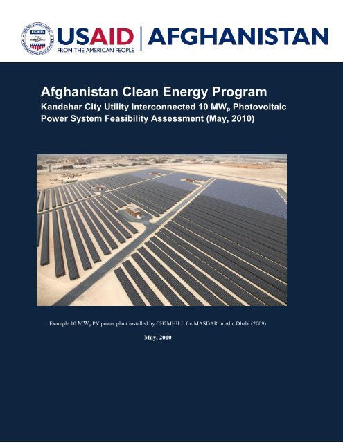
<strong>Afghan</strong>istan Clean Energy Program<br />
<strong>Kandahar</strong> <strong>City</strong> Utility Interconnected 10 MW p Photovoltaic<br />
Power <strong>System</strong> Feasibility <strong>Assessment</strong> (May, 2010)<br />
Example 10 MW p <strong>PV</strong> power plant installed by CH2MHILL for MASDAR in Abu Dhabi (2009)<br />
May, 2010
EXECUTIVE SUMMARY<br />
Scope<br />
The feasibility of a ten MegaWatt (MW p ) photovoltaic power system (<strong>PV</strong>PS) is assessed for <strong>Kandahar</strong><br />
<strong>City</strong> of southern <strong>Afghan</strong>istan.<br />
<strong>System</strong> Performance<br />
The average annual solar resource in <strong>Kandahar</strong> is very good with one axis tracking providing an annual<br />
average of about 5.8 kWh/m 2 /day (sun-hours) at latitude tilt (optimal tilt for maximum annual energy<br />
generation). A large MW scale <strong>PV</strong>PS for <strong>Kandahar</strong> could be installed in approximately 9 months and<br />
serve as a daytime peaking plant. About 40 acres of land are required. An annual <strong>PV</strong> system capacity<br />
factor of 23% was determined. This analysis optimistically assumes that the system is reliable and<br />
operates without long periods of downtime during daylight hours and minimal maintenance actions are<br />
required. It would not provide electricity at night, and installing sufficient energy storage to do so would<br />
double costs, as well as having complicated technical challenges.<br />
Table 1. <strong>Kandahar</strong> 10 MW p Solar <strong>System</strong> Specifications<br />
<strong>System</strong><br />
Economics<br />
Life cycle cost (LCC) analysis is used including all future costs (O&M and replacements). A 10 MW p<br />
solar system would cost about US$75 million to install. It would generate over 20,000 MWh the first year<br />
(about 10 percent of the current <strong>Kandahar</strong> load), and about 48,000 MWh generated over the next 25 years.<br />
LCC value of energy is about 19 cents per kWh.<br />
Table 2. Summary <strong>Kandahar</strong> 10 MW p Solar <strong>System</strong> Expected Performance and Costs<br />
<strong>PV</strong>PS<br />
<strong>PV</strong> Array Size<br />
10 MW<br />
Total Energy Generated (Yr 1) ~20,000 MWh<br />
Total Installed Cost ~$75,000,000<br />
25 Year Net Present Value ~$88,000,000<br />
<strong>PV</strong> Amortized Energy Value $0.19/kWh<br />
Stand-Alone Options<br />
Alternatively, individual solar systems could be installed throughout <strong>Kandahar</strong> <strong>City</strong>. However, costs for<br />
this would approximately double (~US$15/Wp). Thus, 10 MW p of distributed stand-alone systems<br />
throughout the city with batteries would cost over US$150 million. Each system would be as an island<br />
unto itself. Likewise, not as much energy would actually be usable due to ~30% roundtrip efficiency<br />
losses for batteries from charging and discharging. Batteries would need to be replaced every 6-8 years.<br />
2
LCC costs would be more than double for a grid-tied system.<br />
3
1.0 INTRODUCTION<br />
The objective of a proposed 10 MW p <strong>Kandahar</strong> photovoltaic power system (<strong>PV</strong>PS) project would be to<br />
use solar energy to supplement grid power production. A grid-tied <strong>PV</strong>PS allows for generation to meet<br />
some of the daily electrical energy demand during peak hours. The system does not provide power at<br />
night. <strong>PV</strong> systems can also include energy storage, but this extremely expensive for very large grid scale<br />
systems. Thus, photovoltaic (<strong>PV</strong>) power is provided to the grid only during daylight with this type of<br />
system.<br />
Grid-connected <strong>PV</strong>PS are made up of a variety of components, which aside from the <strong>PV</strong> modules, include<br />
conductors, fuses, disconnects, controls, trackers, and power conditioning units (i.e., inverters). The <strong>PV</strong><br />
grid system is only functional when its inverters can operate in synchronization with the regular grid. If<br />
the grid goes down, there is no solar power production.<br />
<strong>PV</strong> systems are modular by nature, thus systems can be readily expanded and components easily repaired<br />
or replaced if needed.<br />
Alternatively, stand-alone off-grid systems could be used in a distributed fashion on individual buildings.<br />
However, costs would approximately double for installation due to batteries.<br />
1.1 Utility Perspectives on Solar Energy Utilization<br />
A utility generating and selling electricity, such as DABS in <strong>Kandahar</strong>, must consider the value of <strong>PV</strong><br />
with respect to the utility's overall objectives. <strong>PV</strong> power could be used to match with demand peak<br />
shaving opportunities. The value of <strong>PV</strong>PS is calculated relative to the opportunity costs. Opportunities<br />
for <strong>PV</strong> for utility planners fall into several categories: Utility-Owned, Off-Grid <strong>System</strong>s; Utility Owned,<br />
Off-Grid, Customer-Service <strong>System</strong>s; Utility-Owned, Grid-Connected Distributed Generation and Line<br />
Support; Customer-Owned, Grid-Connected, On-Site Generation; and Large Scale Utility Applications.<br />
A large scale utility <strong>PV</strong>PS application for <strong>Kandahar</strong> <strong>City</strong> is the most economical option as opposed to<br />
distributed stand-alone systems, and the one focused on here.<br />
DABS is currently providing electric service to the <strong>City</strong> of <strong>Kandahar</strong> and plays an important role in<br />
developing any grid connected <strong>PV</strong> system. Interconnecting a <strong>PV</strong> system to the utility grid is not trivial.<br />
There exist utility interconnection standards for <strong>PV</strong>PS. Inexperienced utilities such as DABS are<br />
generally cautious since they have no experience interconnecting <strong>PV</strong> systems. Most knowledgeable<br />
utilities have adopted IEEE 929-2000 Recommended Practice for Utility Interface of Photovoltaic (<strong>PV</strong>)<br />
<strong>System</strong>s.<br />
1.2 Large Scale Utility Applications<br />
For grid tied <strong>PV</strong>PS applications, the value of <strong>PV</strong> can be compared to the demand profile with the<br />
electrical production, both on a daily as well as annual basis. For this type of application, it is important<br />
that there be a fairly good correlation between the demand and solar generation curves. It is important to<br />
analyze the short-run marginal costs, as well as the long-run marginal costs based on the daily and yearly<br />
cycles. Once these correlations are established, DABS will know how much electricity from the sun can<br />
be expected to meet on-peak demand. <strong>PV</strong> can also improve power quality due to local power load spikes<br />
resulting in short-term overload on transformers and lines, voltage oscillation due to long line runs and<br />
locally varying loads, and poor power quality due to loads with harmonic generating qualities.<br />
Construction Timeframe: The recent 80 kW p <strong>PV</strong>PS installed by SESA in Paktiya took 5 months for<br />
shipping once the order was placed, including 1 month customs clearance. It took about 2 months to<br />
install the system. A larger MW scale <strong>PV</strong>PS will probably take slightly longer to ship and install, so the<br />
system could be operational in approximately 9-12 months after contracting.<br />
4
2.0 PHOTOVOLTAIC (<strong>PV</strong>) BASICS (from Foster, 2009)<br />
It is useful to have a basic technical understanding of solar electric operational concepts to fully<br />
understand this feasibility analysis. Electricity can be produced from sunlight through a process called<br />
photovoltaics (<strong>PV</strong>). "Photo" refers to light and "voltaic" to voltage. The term describes a solid-state<br />
electronic cell that produces direct current electrical energy from the radiant energy of the sun. Solar cells<br />
are made of semi-conducting material, most commonly silicon, coated with special additives. When light<br />
strikes the cell, electrons are knocked loose from the silicon atoms and flow in a built-in circuit,<br />
producing electricity. If a load is connected under these conditions, an electrical current will result, which<br />
is capable of doing work. The current produced is proportional to the amount of light absorbed by the<br />
device. In a solar cell, the photovoltaic effect is manifested as the generation of voltage at its terminals<br />
while being struck by the suns rays.<br />
A thin silicon cell, four inches across, can approximately produce more than one watt of direct current<br />
(DC) electrical power in full sun. Individual solar cells can be connected in series and parallel to obtain<br />
desired voltages and currents. These groups of cells are packaged into standard modules that protect the<br />
cells from the environment while providing useful voltages and currents. <strong>PV</strong> modules are extremely<br />
reliable since they are solid state and there are no moving parts. Silicon <strong>PV</strong> cells manufactured today can<br />
provide thirty or more years of useful service life. Some manufacturers provide warranties of up to 25<br />
years on their <strong>PV</strong> product (at 80 percent of original power rating). For example, a 100 W p <strong>PV</strong> module in<br />
full direct sunlight (1,000 W/m 2 ) operating at 25°C will generate 100 Watts per hour (referred to as a<br />
Watt-hour–[Wh] at rated conditions. Modules can be connected together in series and/or parallel in an<br />
array to provide required voltages and currents for a particular application.<br />
In order to generate usable power <strong>PV</strong> cells are connected together in series and parallel electrical<br />
arrangements to provide the required current or voltage to operate electrical loads. <strong>PV</strong> cells are connected<br />
in series, grouped, laminated, and packaged between sheets of plastic and glass, thus forming a <strong>PV</strong><br />
module. The module has a frame (usually aluminum) that gives it rigidity and allows for ease of handling<br />
and installation. Junction boxes, where conductor connections are made to transfer power from the<br />
modules to loads, are found on the back of the <strong>PV</strong> modules. The number of cells in a module depends on<br />
the application for which it is intended. Terrestrial solar modules were originally designed for charging<br />
12 volt lead-acid batteries, thus many modules are nominally rated at 12 V. <strong>PV</strong> modules designed for<br />
grid-tied application and rated at higher voltages.<br />
<strong>PV</strong> cells essentially operate as diodes. The electrical behavior of <strong>PV</strong> modules is normally represented by<br />
current versus voltage curve (I-V curve). Likewise, a power curve is generated by multiplying current<br />
and voltage at each point on the IV curve. However, the only point desired to operate on this curve is the<br />
maximum power point. Figure 1 shows the IV and <strong>PV</strong> power curves of a representative <strong>PV</strong> module.<br />
5
Figure 1. Typical IV and power curves for a <strong>PV</strong> Module at 1000 W/m 2<br />
Each IV curve has a set of distinctive operation points that should be understood in order to appropriately<br />
install and troubleshoot <strong>PV</strong> power systems.<br />
Short circuit current (I sc ) is the maximum current generated by a cell or module, and is measured when<br />
an external circuit with no resistance is connected (i.e., the cell is shorted). Its value depends on the cell’s<br />
surface area and the amount of solar radiation incident upon the surface. It is specified in Amps and since<br />
it is the maximum current generated by a cell, I sc is normally used for all electrical ampacity design<br />
calculations.<br />
Nameplate current production is given for a <strong>PV</strong> cell or module at standard reporting condition (SRC)<br />
as specified by ASTM. The SRC commonly used by the <strong>PV</strong> industry is for a solar irradiance of 1000<br />
W/m 2 , a <strong>PV</strong> cell temperature of 25C, and a standardized solar spectrum referred to as an air mass 1.5<br />
spectrum (AM=1.5). This condition is also commonly referred to as standard test condition (STC).<br />
However, in reality, unless one is using <strong>PV</strong> in a relatively cold climate, the cells operate much hotter<br />
(often 50°C or more), which reduces their power performance.<br />
Maximum Power Operating Current (I mp ) is the maximum current specified in Amps and generated by<br />
a cell or module corresponding to the maximum power point on the array's current-voltage (I-V) curve.<br />
Open Circuit Voltage (V oc ) is the maximum voltage generated by the cell. This voltage is measured<br />
when no external circuit is connected to the cell.<br />
Rated Maximum Power voltage, V mp . The voltage corresponding to the maximum-power-point on the<br />
array’s current-voltage (I-V) curve.<br />
Maximum Power (P mp ) is the maximum power available from a <strong>PV</strong> cell or module and occurs at the<br />
maximum-power-point on the I-V curve. It is the product of the <strong>PV</strong> current (Imp) and voltage (Vmp).<br />
6
This is referred to as the maximum power point. If a module operates outside of its maximum power<br />
value, the amount of power delivered is reduced and represents needless energy losses.<br />
The power produced by a crystalline <strong>PV</strong> module is affected by two key factors: solar irradiance and<br />
module temperature. The following figure shows how the I-V curve is affected at different irradiance<br />
levels. The lower the solar irradiance, the lower the current output and thus the lower the peak power<br />
point. Voltage essentially remains constant. The amount of current produced is directly proportional to<br />
increases in solar radiation intensity. Basically, V oc does not change; its behavior is essentially constant<br />
even as solar-radiation intensity is changing.<br />
Figure 2. <strong>PV</strong> module current diminishes with decreasing solar irradiance.<br />
The next figure shows the effect that temperature has on the power production capabilities of a module.<br />
As module operating temperature increases, module voltage drops while current essentially holds steady.<br />
<strong>PV</strong> module operating voltage is reduced on average for crystalline modules approximately 0.5 percent for<br />
every degree C above STC (i.e., 25). Thus, a 100 Wp crystalline module under STC now operating at a<br />
more realistic 55 C with no change in solar irradiance will lose about 15 percent of its power rating and<br />
provide about 85 W of useful power. In general when designing <strong>PV</strong> systems, one should expect a fifteen<br />
to twenty percent drop in module power from STC. <strong>Kandahar</strong> CIty will rarely see its <strong>PV</strong> systems operate<br />
at STC conditions and given the hot climate there will be a substantial derate.<br />
7
Figure 3. <strong>PV</strong> module voltage drops with temperature, as does power.<br />
2.1 Grid-Tied <strong>PV</strong> <strong>System</strong>s<br />
A grid-tied <strong>PV</strong>PS only operates when the utility is available. However, in the event of an outage, the<br />
system is designed to shut down until utility power is restored. While a <strong>PV</strong> system can help serve as a<br />
good peak shaving generation system for <strong>Kandahar</strong>, inevitably there will be an overcast day where solar<br />
power production will be much less.<br />
<strong>PV</strong> Array: Consists of <strong>PV</strong> modules interconnected in series and parallel to obtain the desired voltage and<br />
current. All <strong>PV</strong> modules should be IEC or UL listed and installed in accordance with National Electrical<br />
Code (NEC) guidelines (UL & NFPA, 2008)<br />
Balance of <strong>System</strong> components (BOS): BOS includes mounting systems and wiring systems. The wiring<br />
systems include disconnects for the dc and ac sides of the inverter, ground-fault protection, and<br />
overcurrent protection for the solar modules. Most systems include a combiner board of some kind since<br />
most modules require fusing for each module source circuit.<br />
Power Conditioning Unit: This is the device (i.e., inverter) that takes the dc power from the <strong>PV</strong> array and<br />
converts it into standard ac power for the grid.<br />
Monitoring: Metering that indicates system performance and assists with operation.<br />
2.2 Array Mounting Options<br />
<strong>PV</strong> systems can produce as much as 10 Watts per square foot of array area. Typically, about 36,000<br />
square feet (400’ x 90’) per 200 kw (ac output) of unobstructed area is used for tracking <strong>PV</strong> crystalline<br />
8
systems for a typical area in the feasibility study (or ~16.7 m 2 per kW). About half this for lower<br />
efficiency thin-film technologies. Typically, anywhere from 1,700 (x-Si) to 3,000 (a-Si) square meters per<br />
100 kW (ac output) of unobstructed area is required, depending on module type and tracking used. The<br />
final actual area will depend on the type of modules and tracking system selected and their efficiencies.<br />
For <strong>Kandahar</strong> latitude, will need about 40 acres for a 10 MW one axis (E-W) tracking system using<br />
crystalline <strong>PV</strong> technologies.<br />
2.2.1 Roof mount<br />
<strong>PV</strong> arrays of a few kiloWatts are often mounted on individual rooftops. The weight of the <strong>PV</strong> array is<br />
typically about 5 lbs/ft 2 . Depending on structure, this can be the most inexpensive mount for an array for<br />
an existing substrate. Sometimes, such as with flat roofs commonly found in <strong>Afghan</strong>istan, a separate<br />
structure with a more optimal tilt angle is mounted on the roof. Proper roof mounting is labor intensive.<br />
Particular attention should be given to the roof structure and the weather proofing of roof penetrations.<br />
Typically, there is one support bracket for every 100 Watts of <strong>PV</strong> modules. There are also additional<br />
building shade issues.<br />
Generally speaking, roof mounted <strong>PV</strong> arrays are most typically less than 10 kW in size. There are only a<br />
few rooftop <strong>PV</strong> arrays in the hundreds of kW range. Rooftop arrays are more complicated to plan for<br />
large MW systems and only make sense for very large buildings and rarely exceed 1 MW in size (e.g., an<br />
airport terminal). To plan out multiple small rooftop installations throughout <strong>Kandahar</strong> <strong>City</strong> will be very<br />
difficult and expensive to implement and operate. Each individual system would need its own inverter,<br />
therefore driving up overall system costs. Likewise, experience has shown in Japan and the U.S. that if<br />
there are many small systems (hundreds), grid stability suffers as overall grid voltage tends to drift<br />
upward due to the interaction of many small inverters.<br />
2.2.3 Ground Mount<br />
A ground mounted <strong>PV</strong> array is the least expensive and most viable option for a 10 MW <strong>Kandahar</strong> <strong>PV</strong>PS<br />
from a logistics, budget, operational, and planning perspective. The required size for a 10 MW <strong>PV</strong> 1 axis<br />
tracking array is about 167,000 square meters (roughly 40 acres). The vendor will have to create the<br />
substrate for the <strong>PV</strong> installation, which requires somewhat extensive civil works to install. A single<br />
ground-mounted system with a few large inverters is the best option for <strong>Kandahar</strong> city for a large 10 MW<br />
grid interactive <strong>PV</strong>PS.<br />
2.3 <strong>System</strong> Output Considerations<br />
For a large <strong>Kandahar</strong> <strong>PV</strong>PS, the <strong>PV</strong> array will provide power to the power grid via a few utilityinteractive<br />
inverters (or power conditioning unit, PCU). <strong>PV</strong> systems produce power in proportion to the<br />
intensity of sunlight striking the solar array surface. The intensity of light on a surface varies throughout<br />
a day, as well as day to day, so the actual output of a solar power system varies substantially over a day.<br />
There are other factors that affect the output of a solar power system. DABS should understand these<br />
variables so as to have realistic expectations of overall system output and economic benefits under<br />
variable weather conditions. It is important to think in terms of overall system design. A <strong>PV</strong> system<br />
should be engineered to work together as a unit. Thus, good <strong>PV</strong> system designers think in terms of<br />
overall system design and systemic operational performance. For the <strong>Kandahar</strong> project, <strong>PV</strong> system<br />
interaction with the existing grid will need to be evaluated.<br />
2.3.1 Output Factors - Standard Test Conditions<br />
<strong>PV</strong> modules produce dc electricity. The dc output of solar modules is rated under Standard Test<br />
Conditions (STC). These conditions allow for consistent comparisons of products, but need to be<br />
modified to estimate output under common outdoor operating conditions. STC conditions are:<br />
solar cell temperature = 25 °C;<br />
solar irradiance = 1000 W/m 2 ; for a<br />
9
solar spectrum through 1.5 thickness of atmosphere (ASTM Standard Spectrum).<br />
A solar module will be rated at a given output, e.g., 100 Watts of power, under STC. Modules<br />
often have a production tolerance of +/-5 percent of this rating in actuality.<br />
2.3.2 Temperature<br />
Module output power reduces as module temperature increases. A solar module will heat up substantially<br />
above ambient temperature, often reaching operating temperatures of 50-75 °C. For crystalline modules,<br />
a typical temperature reduction factor is about .05 percent per °C above 25°C. For the <strong>Kandahar</strong> analysis,<br />
the monthly average maximum temperature is used to calculate the daily average module operating<br />
temperature is estimated as follows (Pate, 1992):<br />
Where Tm – module operating temperature °C<br />
Ta - ambient temperature °C<br />
Tm = 20.4 + 1.2(Ta)<br />
2.3.3 Environmental Factors<br />
Key environmental factors affecting <strong>PV</strong> system performance are total solar energy available and module<br />
operating temperature. For the <strong>Kandahar</strong> analysis, 1 axis E-W tracking of the <strong>PV</strong> arrays are assumed<br />
using solar energy data (NREL). <strong>PV</strong> modules are assumed to conservatively operate in ambient<br />
temperatures equal to the average daily maximum high temperature for each month.<br />
Table 3: <strong>Kandahar</strong> Insolation and Average Daily Maximum Temperature<br />
Month<br />
1 Axis Tracking Latitude<br />
Tilt kWh/m2/day<br />
Avg Daily<br />
Max Temp °C<br />
January 4.0 13.0<br />
February 5.3 17.0<br />
March 6.7 22.0<br />
April 8.8 28.0<br />
May 9.9 33.0<br />
June 12.3 37.0<br />
July 11.5 39.0<br />
August 9.8 37.0<br />
September 8.9 34.0<br />
October 6.9 29.0<br />
November 4.6 23.0<br />
December 3.7 25.0<br />
Average 7.7 28.1<br />
2.3.4 Mismatch and wiring losses<br />
For the dc side of the system, the maximum power output of the total <strong>PV</strong> array is always less than the<br />
sum of the maximum output of the individual modules. This difference is a result of slight<br />
inconsistencies in performance from one module to the next and is called module mismatch and amounts<br />
to at least 2 percent loss in system power. Power is also lost to resistance in the system wiring. These<br />
losses should be kept to a minimum but it is difficult to keep these losses below 3 percent for the system.<br />
For purposes of the <strong>Kandahar</strong> analysis, such losses are considered to be a total of four percent for the dc<br />
side of the system and included in the analysis.<br />
2.3.5 dc to ac conversion losses<br />
The dc power generated by the solar module must be converted into ac power using an inverter. Some<br />
10
power is lost in the conversion process, and there are additional losses in the wires from the array to the<br />
inverter and out to the grid. Inverters commonly used in <strong>PV</strong>PS have peak efficiencies of 92-94 percent<br />
indicated by their manufacturers laboratory conditions. Actual field conditions usually result in overall<br />
dc-to-ac conversion efficiencies of about 88-92 percent. For the <strong>Kandahar</strong> analysis, an average of 90<br />
percent conversion efficiency is considered.<br />
2.4 <strong>System</strong> Warranties<br />
There are several types of warranties available for <strong>PV</strong> systems. These include (a) product warranties<br />
covering defects in manufacture; (b) system warranties covering proper operation of equipment for a<br />
specific time period (e.g., 10 years); and, (c) annual energy performance warranties covering the<br />
guaranteed output of the <strong>PV</strong> system. The vendor, to guarantee proper system installation, should be asked<br />
to cover the system and annual energy performance warranties. A typical system level warranty might<br />
state that the <strong>PV</strong> system is guaranteed to produce X kilowatts of AC power at <strong>PV</strong>USA Test Conditions<br />
(PTC) (PTC is 1kW/m2 irradiance, 1 m/s wind speed, 20°C ambient temperature) in the fifth year of<br />
operation.<br />
2.4.1 Product Warranties<br />
<strong>PV</strong> modules may have warranties for as much as 25 years by some manufacturers. However, there are<br />
many other components in <strong>PV</strong> systems that will not have the same life expectancy. Inverters may have a<br />
warranty of ten years or less. DABS should look also closely at the individual product warranties.<br />
2.4.2 Performance Warranties<br />
An energy performance warranty guarantees that the system will perform consistently over a period of<br />
time. This is particularly helpful in ensuring that <strong>Kandahar</strong> receives the bill savings expected. Adequate<br />
metering to verify the system power output and energy generation is necessary to understand whether the<br />
system is operating properly, or has warranty-related performance issues. With an adequate metering<br />
system, <strong>Kandahar</strong> can identify when the system is malfunctioning. There are a few <strong>PV</strong> companies selling<br />
systems with this type of warranty for larger systems.<br />
3.0 GENERAL <strong>PV</strong> SYSTEM PERFORMACE ANAYLSIS<br />
3.1 <strong>Kandahar</strong> Electric Generation<br />
A utility-interactive <strong>PV</strong>PS for <strong>Kandahar</strong> in southern <strong>Afghan</strong>istan is proposed to provide power for the city<br />
load. The city, which is home to about 850,000 people, receives about 16-24 MW of power (this<br />
represents only 20-30 Watts per person!). Currently, approximately 10-12 MW is coming from Kajaki<br />
Dam, 7 MW for 24/7 power is generated by KTA50 Diesel gensets, and 7 MW for 24/6 is generating by<br />
QSK60 gensets. The QSK60 gensets are generating power for <strong>Kandahar</strong> for 24/16 if the Kajaki –<br />
<strong>Kandahar</strong> transmission line is off. Therefore, the daily energy production in <strong>Kandahar</strong> is under 500<br />
MWh/day (Wardak, 2010). Military officials estimate potential demand at about 50 MW (Washington<br />
Post, 2010).<br />
Electricity tariffs for <strong>Kandahar</strong> are way below cost, especially given the limited generation. DABS only<br />
charges users Af 3.00 per kWh (or ~US$.06/kWh). Thus, the value of the electricity generated in<br />
<strong>Kandahar</strong> is heavily subsidized and there simply is not nearly enough electricity to meet the demand.<br />
Diesel generated electricity is probably running over 40 cents per kWh. Hydropower (Kajaki Dam) is<br />
always the cheapest long term electricity solution.<br />
11
3.2 <strong>System</strong> Capacity Determination<br />
<strong>System</strong> capacity defines the <strong>PV</strong> system's generating capacity. Among the items to consider are the <strong>PV</strong><br />
capacity and inverter capacity. Regardless of the system being considered, it is important for the system<br />
design and capacity (<strong>PV</strong> and alternatives) to guarantee the same reliability of supply. For the <strong>Kandahar</strong><br />
analysis, it is assumed that the <strong>PV</strong> system is going to help provide a portion of the city load during<br />
daylight hours only (there is no energy storage).<br />
3.3 <strong>PV</strong> <strong>System</strong><br />
Tracking Method: 1-axis E-W tracking<br />
Array Slope: 32° (~latitude tilt for <strong>Kandahar</strong> – maximum annual energy production)<br />
Array Azimuth: 0 ° (due south)<br />
3.3.1 <strong>PV</strong> <strong>System</strong> Component Efficiencies:<br />
Modules: Temperature derate of 0.5% per °C above 25°C using the average monthly daily max average<br />
temperature as a base.<br />
PCU: 90% average efficiency<br />
Total wire, switchgear, fuses, mismatch losses: 5%<br />
Total Average <strong>PV</strong> <strong>System</strong> Efficiency: 75% on average for the first year, varies by month and dependent<br />
on ambient temperature.<br />
3.3.2 <strong>PV</strong> Array Degradation<br />
<strong>PV</strong> modules degrade slightly each year. For this analysis, the <strong>PV</strong> array was considered to degrade at an<br />
average rate of 0.8% each year. After 25 years, total array degradation is expected to be 20% below<br />
nameplate rating. This is typical of the warranty offered by several manufacturers (e.g., Sharp). Actual<br />
<strong>PV</strong> array degradation will vary by climate and module manufacturing methods.<br />
3.3.3 <strong>PV</strong> Plant Capacity Factor: This represents the total 24 hour operating capacity for the <strong>PV</strong><br />
plant, which give <strong>Kandahar</strong> solar resource is considered as ~23 percent for the first year. This assumes no<br />
significant downtime for maintenance. This range of capacity factor has been met by other large <strong>PV</strong> grid<br />
tied plants in similar desert regions in the U.S. and Middle East. This factor will gradually decline over<br />
time as the array gradually degrades, maintenance actions, etc.<br />
3.4 Energy Production<br />
Energy production for the <strong>Kandahar</strong> solar electric system can be estimated given the solar resource for<br />
<strong>Kandahar</strong> and ambient termperature. Note that solar resource can vary as much as ten percent from year<br />
to year (especially due to global volcanic activity in the northern hemisphere). For the proposed <strong>Kandahar</strong><br />
10 MW solar electric system, it was estimated that given an average meteorological year is should<br />
generate about 20,183 MWh during the first year of operation. Average expected <strong>PV</strong> plant size for<br />
<strong>Kandahar</strong> are provided in Table 4.<br />
There are three calculated parameters commonly applied to <strong>PV</strong> systems: availability; energy production;<br />
and capacity factor. <strong>System</strong> availability is the ratio of the time the <strong>PV</strong> system is producing energy to the<br />
time sunlight is available. A plant that produces between sunrise and sunset is 100% available, and no<br />
penalty for sundown is imposed. Availability relates to system or plant reliability but is not of great value<br />
to planners determining a utility-wide application. <strong>PV</strong> plants are modular, and a plant is deemed available<br />
even when it is only partially on-line. For the <strong>Kandahar</strong> analysis, the system is optimistically always<br />
considered to be available. This is a best case assumption and in reality there will probably be downtime<br />
periods for parts of the system during daylight hours.<br />
12
Table 4: <strong>Kandahar</strong> <strong>PV</strong>PS Specifications<br />
Capacity factor is the ratio of the <strong>PV</strong> energy produced in a given time to the energy that could be<br />
produced in that time if the plant had been continuously generating its fully rated output. Because <strong>PV</strong><br />
plants can only produce during daylight hours and output is reduced to heat, a capacity factor of about<br />
23% is realistic for southern <strong>Afghan</strong>istan for crystalline <strong>PV</strong> modules. Similar installed utility <strong>PV</strong> power<br />
plants in the Southwest U.S. and Middle East operate at about this same capacity factor.<br />
Fig.<br />
4.<br />
QuickTime and a<br />
decompressor<br />
are needed to see this picture.<br />
<strong>Kandahar</strong> Estimated <strong>PV</strong> Power <strong>System</strong> Plant Capacity Factor by Month<br />
13
Fig.<br />
5. 10<br />
MW<br />
QuickTime and a<br />
decompressor<br />
are needed to see this picture.<br />
<strong>Kandahar</strong> <strong>PV</strong>PS Plant Monthly kWh Generated (Year One)<br />
Table 5: <strong>Kandahar</strong> 10 MW <strong>PV</strong>PS Plant Performance Summary (Year One)<br />
14
Over time, the <strong>PV</strong> arrays will gradually degrade and performance and energy production will likewise<br />
drop. Actual <strong>PV</strong> array degradation varies depending on installation, environment, and modules used. The<br />
<strong>Kandahar</strong> <strong>PV</strong>PS is assumed to degrade within <strong>PV</strong> module manufacturer specifications of providing 80<br />
percent of rated power after 25 years, which implies an annual module degradation rate on average of 0.8<br />
percent per year. The figure below tracks expected annual <strong>Kandahar</strong> performance trends for an average<br />
meteorological year. Actual performance will vary. Total 25 year expected energy production is<br />
approximately 472 million kWh. Actual production will vary with insolation, ambient temperature, and<br />
overall <strong>PV</strong> plant availability.<br />
Fig.<br />
6.<br />
QuickTime and a<br />
decompressor<br />
are needed to see this picture.<br />
Expected 10 MW <strong>PV</strong>PS plant annual energy generation over 25 years.<br />
15
4.0 KANDAHAR <strong>PV</strong>PS ECONOMICS<br />
In order to understand the economics of a large-scale <strong>PV</strong> power system (<strong>PV</strong>PS), it is imperative to<br />
conduct financial analyses of such a system as compared to conventional alternatives on a life-cycle cost<br />
basis. <strong>PV</strong> modules are guaranteed by manufacturers up to 25 years of 80% of rated wattage at standard<br />
test conditions (25°C and 1,000 W/m 2 ). The useful module lifetime is probably actually 35 years or<br />
more, although the actual end of life mechanism for <strong>PV</strong> modules (Block V modules) is still unknown as<br />
the oldest modules of the type currently produced have only about 30 years of operation to date. Long<br />
term lifetime for many thin film modules is even less known as most have less than a decade in<br />
production. Thus, when a user purchases a <strong>PV</strong> array, they are actually purchasing the equivalent of 40<br />
years or more of power production. The only way to make a fair economic assessment of the equipment<br />
is to look at a levelized life-cycle cost analysis over a reasonable time frame.<br />
Any solar project subjected to financial evaluation will have its costs and benefits spread out over a<br />
number of years. In order to compare one project with another, or to determine the financial viability of a<br />
particular project, it is necessary to streamline the costs and benefits to a single number over time. This is<br />
most easily done by calculating the present value. There are a variety of methods used for calculating<br />
financial feasibility of solar energy projects. For life-cycle cost comparison considered here, the Net<br />
Present Value (N<strong>PV</strong>) method of comparison is most easily applied and commonly used for this type of<br />
analysis.<br />
4.1 Net Present Value Method<br />
The N<strong>PV</strong> of any particular investment project (solar, etc.) at the point in time for t = 0 is the sum of the<br />
present values of all the cash inflows and outflows related to the investment. Expenditure and income are<br />
generally balanced to obtain annual returns so that the N<strong>PV</strong> of an investment is simply the sum of the<br />
present values of its return plus the present value of its liquidation yield less the present value of its<br />
investment costs:<br />
N<strong>PV</strong> = annual returns - investment costs + liquidation yield<br />
An investment project is only profitable when its N<strong>PV</strong> is greater than or equal to zero. When there are<br />
several alternative investment possibilities (e.g., investing in a <strong>PV</strong> system or a wind energy system), the<br />
N<strong>PV</strong> of the different projects can be compared with one another and investment with the highest N<strong>PV</strong><br />
selected.<br />
5.0 LIFE CYCLE COSTING METHODOLOGY (LCC)<br />
It is reasonable to use a life cycle cost approach, particularly when dealing with renewable energy<br />
technologies which typically have high initial capital costs, as opposed to conventional energy sources<br />
which typically have relatively low capital cots, but high operational and maintenance costs. Electrical<br />
generation costs can be classified under different criteria. The costs for electrical generation can be<br />
broken out into five main categories:<br />
• Capital costs<br />
• Operation and Maintenance Costs<br />
• Fuel Costs<br />
• Replacement Parts Costs<br />
• Environmental Costs<br />
Depending on the type of power production required, these costs will vary. For instance, if coal or oil<br />
electrical generation plants are compared to a utility scale <strong>PV</strong> energy system, the initial costs of the fossil<br />
fuel based plants per MW are lower, the operation and maintenance costs and fuel costs are relatively<br />
16
high. Conversely, <strong>PV</strong> systems have high initial costs but zero fuel costs and low operation and<br />
maintenance costs.<br />
Thus, viable economic decisions cannot be made only on the basis of one type of costs (e.g., capital cost),<br />
but rather must consider all the costs incurred over the lifetime of the system. Levelized life cycle costing<br />
(LCC) analysis methods make it possible to compare different alternatives by adding up the project costs<br />
over its lifetime.<br />
The life cycle cost (LCC) method of economic analysis calculates a system's total cost over its useful life.<br />
This method takes into account the initial (capital) outlays and all other costs required for the system to<br />
operate properly over its life. The LCC method helps quantify the economic impacts of a project using<br />
different cost components with varying reliability factors. It helps optimize the overall system analysis<br />
from a traditional economic standpoint. It also allows a method to assess the impact of changing<br />
economic variables such as interest rates and inflation. While it is very difficult to accurately predict how<br />
these variables will change in the future, it does provide a relatively good method to assess impacts based<br />
on what the most likely future assessment for these variables is. The LCC can be calculated as follows:<br />
where,<br />
LCC = Cpv + O&Mpv + Fpv + Rpv + Epv - Spv<br />
Capital investment (Cpv) present value is the cost of equipment, including systems design and<br />
installation costs. This is a one-time payment at the start of a project. Various investment costs for a <strong>PV</strong><br />
system can be indexed according to their time of accrual in ways that make it possible to order the<br />
investment expenditures clearly, according to a time schedule as is needed for the proper calculation of<br />
financial acceptability of a project. Typical investment costs are as follows, most of which are applicable<br />
to <strong>Kandahar</strong>:<br />
Possible <strong>Kandahar</strong> Applicable <strong>PV</strong> <strong>System</strong> Costs<br />
• Planning/Administrative<br />
• Environmental impact studies<br />
• Land acquisition/leasing<br />
• Civil works (e.g., <strong>PV</strong> structure)<br />
• Plant building/structures (power house)<br />
• Machinery (e.g., inverters)<br />
• Utility connections (e.g., roads, grid interconnects)<br />
• Shipping/transportation including insurance<br />
• Assembly and commissioning<br />
• Taxes, custom duties, fees<br />
• Other costs (e.g. security)<br />
<strong>PV</strong> project costs are determined from reported industry averages, with <strong>PV</strong> modules representing about a<br />
third of project costs. Large grid interconnected <strong>PV</strong> systems in the Southwest U.S. ad the Middle East<br />
typically range from a low of about $6.00/Watt and a high of $8.00/Watt. Costs vary with location,<br />
vendor, system size, module technology, local labor rates, contractor experience, insurance, etc.<br />
The largest regional grid-tied <strong>PV</strong>PS is the recent 2009 Masdar Abu Dhabi 10 MW p installation by<br />
CH2MHILL shown on the front cover. This single-axis tracking <strong>PV</strong> system cost US$6/Wp ( 5 MW p First<br />
Solar CdTe modules and 5 MW p x-Si). Thin-film (e.g., a-Si) <strong>PV</strong> modules take about double the area for<br />
the same power production as compared to crystalline (x-Si) modules due to lower conversion<br />
efficiencies.<br />
17
However, projects always cost more in <strong>Afghan</strong>istan due to security issues, difficult logistics, overland<br />
shipping, etc. With shipping and logistics, the recent Paktiya 80 kW p fixed array x-Si <strong>PV</strong> system installed<br />
by SESA in Jan. 2010 cost US$2.3 million (including ~$800k for battery bank and ~$700k for<br />
transmission). Thus about $10.00/Wp without energy storage and transmission. A larger MW sized <strong>PV</strong>PS<br />
will have greater economies of scale. However, since no such project has ever been undertaken in<br />
<strong>Afghan</strong>istan, actual costs will<br />
Thus, a <strong>Kandahar</strong> MW size <strong>PV</strong>PS should cost somewhere between the Abu Dhabi and Paktiya examples<br />
cited. For this analysis, ~US$7.50/Wp +/- 20% is probably is assumed to be a reasonable installed cost<br />
estimate for a 10 MW p scale grid-tie installation with single-axis tracking for <strong>Kandahar</strong>.<br />
Thus, about US$75 million +/- 20% would be a reasonable expected installed cost for a 10 MWp<br />
<strong>Kandahar</strong> <strong>PV</strong>PS. This excludes transmission needed to move the power. Costs for this will be dependent<br />
on the location for the MW system. Ideally, a flat open publically owned land site of approximately 40<br />
acres chosen near existing transmission or power plant is where to install such a large system to keep<br />
transmission costs to a minimum.<br />
Operation and Maintenance costs (O&Mpv) present value is the total sum of annual costs taken as a<br />
present worth for operator's salaries, equipment inspections, insurance, tax, prepaid maintenance. These<br />
costs here are not reflecting the cost of fuel consumption or replacing major equipment items.<br />
Estimations of personnel costs over the project lifetime, particularly in labor-intensive projects of long<br />
duration can be an important component of any LCC analysis. It is necessary to carefully consider any<br />
increase in these costs on the basis of the anticipated general inflation rate. If opportunity costs of selfemployment<br />
become significant, these should also be accounted for by an appropriate sum in the financial<br />
evaluation.<br />
The actual expenses related to maintaining and servicing a <strong>PV</strong> or other plant can vary greatly, thus in<br />
practice it is very difficult to accurately predict what these costs will be. This type of comparison should<br />
also be done in light of what the DABS on-site staff are capable of carrying out themselves with local<br />
parts. In practice, a best guess based on previous experience with similar equipment in the Southwest<br />
U.S. and Middle East region should be made for estimating annual maintenance and repair costs. For the<br />
<strong>Kandahar</strong> analysis, an annual maintenance cost of $12,000 per MW is reported for maintenance including<br />
replacements for DOD <strong>PV</strong> power plants (Black, 2003). The military DOD experience is probably most<br />
analogous to the proposed <strong>Kandahar</strong> <strong>PV</strong>PS case. General annual maintenance outside of replacements is<br />
considered to be .012/kW installed for this analysis, which essentially covers the equivalent of one full<br />
time maintenance person for the <strong>Kandahar</strong> 10 MW <strong>PV</strong> system.<br />
Fuel cost (Fpv) present value is the total expenditures for fuel consumed by the system. These costs vary<br />
at a rate often quite different from operation and maintenance costs. Grid electricity price for <strong>Kandahar</strong> is<br />
assumed to escalate at an average 1 percent per year in addition to the real discount rate. Obviously, there<br />
are no fuel costs for the <strong>Kandahar</strong> <strong>PV</strong>PS.<br />
Replacement costs (Rpv) present value reflect major repairs and equipment replacements which occur<br />
when the normal duty life of any system components is shorter than the life expectancy of the entire<br />
system. For the <strong>Kandahar</strong> analysis, the PCU is assumed to be replaced halfway through the system<br />
lifetime (i.e., 12.5 years).<br />
Environmental costs (Epv) present value are those costs not normal reflected in conventional economics<br />
that take into account the externalities associated with environmental damage and risks. For some<br />
analysts, they may not be allowed to use this very real cost since these costs are often not borne directly<br />
18
y the user, but by society as a whole. For the <strong>Kandahar</strong> <strong>PV</strong>PS analysis, environmental costs are<br />
excluded.<br />
Salvage value (Spv) present value or recovery value of the equipment is the net value of the equipment<br />
used at the end of the system's service life. The salvage or residual value of a plant and/or components is<br />
based on the possibilities of alternative uses at the end of the project lifetime. Assuming that equipment<br />
or plant parts can be sold, the expected liquidation yield from the sale at a fixed point in time is usually<br />
taken as the residual value. If a later sale is improbable, than a salvage value of zero would be<br />
appropriate. Any possible dismantling costs and costs for making a sale must be deducted from the<br />
project salvage value. For the <strong>Kandahar</strong> <strong>PV</strong>PS, the salvage value after 25 years are assumed to be zero.<br />
When applying LCC methodology, it is easiest to evaluate all costs from different years correlated to one<br />
year (e.g., net present value). Costs that arise in the future must be discounted due to the time value of<br />
money. Typically, all future costs are transformed to their present value. Appropriate discount factors<br />
must be applied to this end as can be commonly found in many financial tables or formulas. To calculate<br />
present worth, the following equation is used:<br />
<strong>PV</strong> = FV/(1+i) n<br />
where<br />
<strong>PV</strong> = Present Value<br />
FV = Future Value<br />
i = interest rate<br />
n = number of years<br />
Other factors such as annuity type costs require similar calculations as well. For instance, to calculate the<br />
present worth where annual payments are known and the total present worth of all payments needs to be<br />
determined, the following equation can be used:<br />
where A = annuity payment<br />
UPW = Uniform Present Worth<br />
<strong>PV</strong> = A * UPW<br />
UPW = [(1 + i) n - 1]/i(1 + i) n<br />
Choosing realistic discount rates will be the most difficult and one of the most influential variables in the<br />
LCC analysis. If a low discount rate is chosen, this will emphasize future costs, since they will be<br />
discounted less than the initial costs, as opposed to a high discount rate which emphasizes initial costs<br />
over future costs. The discount rate should reflect the system owner's potential for saving funds in<br />
conventional economic terms. It is important to note that the nominal investment rate is not the effective<br />
rate of return received by the end-user since this if affected by inflation and will reduce the value of future<br />
savings. Thus, it is important to subtract the inflation rate from the nominal investment rate to obtain the<br />
real discount rate. Since the fossil fuel inflation rate is often higher than that of products, it is reasonable<br />
to assume a separate fuel escalation rate as well.<br />
5.1 Economic Parameters for LCC Analysis<br />
For any type of economic analysis, the critical economic parameters and type of financial analysis<br />
procedure for the analysis must be carefully thought out. This is an inexact task in that it requires making<br />
estimations about the future.<br />
19
Project Lifetime<br />
The service life of an installation is the number of years beyond which the system becomes more<br />
expensive to maintain than a new acquisition or when the efficiency of the system deteriorates such that<br />
the output product is unacceptable in quality and/or quantity. There are several different methods to<br />
estimate the useful service life of capital assets. The more sophisticated methods use actuarial analysis,<br />
while other methods that are more convenient and simple use national tax guidelines. The service lives<br />
used as the basis for depreciation accounting should be determined by the asset's particular operating<br />
conditions and experience. Actuarial approaches to estimating service life are more involved and consist<br />
of construction of frequency curves, survivor curves and probable-life curves. For this analysis, a total <strong>PV</strong><br />
project lifetime was assumed to be 25 years, at the end of which the <strong>PV</strong> system would be providing 80<br />
percent of its nameplate power rating.<br />
Inflation Rate<br />
Inflation is the increase of prices paid for goods and services over time. The increase in prices results<br />
from either cost inflation or price inflation or some combination thereof. Cost inflation is the result of a<br />
real cost increase to produce goods and services. Price inflation may be caused by an increase in the<br />
amount of money held in a national economy. It may also be caused by the speed and spending habits of<br />
people within a society. Thus, cost inflation and price inflation can occur at the same time, causing the<br />
value of money to change at different times.<br />
Government's use price indexes to track the value of money over time. Wholesale Price Indexes and<br />
Consumer Price Indexes are used which cover specific types of products. Inflation is normally expressed<br />
as an annual percentage over a time period. The annual rate of inflation can be determined by<br />
f(t) = - (PIt / PIto) - 1<br />
where<br />
f(t) = annual inflation rate<br />
PIt = current price index<br />
PIto = reference year price index<br />
<strong>Afghan</strong>istan has experienced relatively low inflation over the past few years, typically only a few percent<br />
per year. For the <strong>Kandahar</strong> analysis, an average annual inflation rate of 3 percent was used as a<br />
projection for the next 25 years.<br />
Discount Rate<br />
In determining the financial viability of solar energy projects, one of the logical manners to determine this<br />
is to reduce the time stream of costs and benefits to a single number by calculating the net present value<br />
(N<strong>PV</strong>) of the project. For any single project the discount rate will affect whether the N<strong>PV</strong> is greater or<br />
less than zero. For comparing projects, the discount rate will affect the N<strong>PV</strong> ranking.<br />
Ideally, the correct discount rate is the rate when applied to future costs and benefits yields the actual<br />
present social values. Thus, this is the rate at which society as a whole is willing to trade off the present<br />
for future costs and benefits. The choice of a proper rate is not over numerical values per se, but rather<br />
concerns the idea of what the discount rate should measure.<br />
The critical discount rate is that where the N<strong>PV</strong> of a project changes sign. Sensitivity analysis can be<br />
helpful to determine how critical the discount rate of a project is. Following are the different types of<br />
rates that can be considered for project development.<br />
20
Real Discount Rate<br />
Once the most appropriate discount rate category has been selected (e.g., corporate rate or market interest<br />
rate), the real discount rate is calculated as the difference between the discount rate and the inflation rate.<br />
For the <strong>Kandahar</strong> analysis, the final real discount rate used is 1 percent.<br />
Fuel Escalation Rate<br />
For the <strong>Kandahar</strong> <strong>PV</strong>PS, it can be assumed that solar power will be directly available in the required<br />
quantity and quality, free of charge, after the installation of the necessary plant and equipment for the<br />
project site. When using grid power sources, additional costs arise for the procurement, transport,<br />
processing and storage of the relevant energy source for fueling the plant, as well as any costs associated<br />
with discarding or discharging residues within legal requirements are already included in the grid price of<br />
electricity. The present worth of grid power over the project lifetime needs to be calculated.<br />
The determination of the annual energy escalation rate is based on the price index of the particular energy<br />
source in question. The energy escalation rate can also be calculated from the expected real increase in<br />
the cost of energy and the general inflation rate as follows:<br />
e(t) = [1 + e * (t)][1 + f(t)] - 1<br />
where<br />
e(t) = annual energy escalation rate<br />
e * (t) = real annual rate of increase in the cost of energy<br />
For the <strong>Kandahar</strong> <strong>PV</strong>PS, an average annual grid electricity modest price increase of two percent per year<br />
was assumed over the next 25 years. Obviously current subsidized electricity tariffs in <strong>Kandahar</strong> cannot<br />
be maintained. It’s possible actual price increases could be much more and will depend on what happens<br />
with the Kajaki hydropower system.<br />
Externalities<br />
LCC methodology generally is not used to incorporate externalities related to energy production and<br />
usage. However, probably the best single way to incorporate externalities for an LCC analysis is by<br />
assigning additional costs (or subsidies) to the fuel source in question. The difficult part is in assigning a<br />
value of improved security, reduced emissions, spill risks, noise pollution, etc. No externalities are<br />
included for this analysis.<br />
6.0 <strong>Kandahar</strong> <strong>PV</strong>PS LCC Analysis<br />
The following analysis is a life-cycle cost estimate for the proposed <strong>Kandahar</strong> 10 MW p grid-tied <strong>PV</strong>PS as<br />
compared to the conventional electric grid. The LCC analysis has been conducted assuming average<br />
annual production with normal <strong>PV</strong> system losses based on one axis tracking at latitude tilt No salvage<br />
value has been given to either the grid or <strong>PV</strong> systems, although in reality used <strong>PV</strong> modules could be<br />
worth as much as 20% or more of their original value at the end of 25 years. No externalities are<br />
assumed.<br />
21
Economic Conditions<br />
The useful lifetime for the <strong>Kandahar</strong> grid-tied <strong>PV</strong>PS is assumed to be 25 years using net present value<br />
life-cycle cost analysis over a 25 year lifetime. Actual project development costs for southern<br />
<strong>Afghan</strong>istan could vary by as much as 20 percent from those estimated here. However no MW scale <strong>PV</strong><br />
arrays have been installed in <strong>Afghan</strong>istan and the nearest such type installations are in UAE. So final<br />
costs could vary depending on local factors and costs. The following table details the common base case<br />
financial assumptions.<br />
Large grid interconnected <strong>PV</strong> systems have been installed at a range of costs. <strong>System</strong> costs, especially for<br />
ground mounted systems with extensive civil works, are typically between US$6-8 per installed peak<br />
Watt (Wp). For the <strong>Kandahar</strong> <strong>PV</strong>PS cost estimate, an installed cost is assumed to be US$7.50 per<br />
installed Watt.<br />
6.2 <strong>Kandahar</strong> Financial Assumptions:<br />
Table 6. <strong>Kandahar</strong> 10 MW p <strong>PV</strong> Economic Assumptions<br />
Parameter<br />
Solar <strong>System</strong><br />
Project Lifetime<br />
25 years<br />
Salvage Value<br />
none<br />
Installation Cost<br />
$7.50/Wp<br />
Fuel Cost<br />
none<br />
Demand Cost<br />
none<br />
Fuel (Grid) Escalation Rate<br />
2% per year<br />
O&M Costs<br />
$.012/kW installed per year<br />
General Inflation<br />
3% per year<br />
Discount Rate<br />
2% per year<br />
Real Discount Rate<br />
1% per year<br />
The LCC analysis was conducted to bring all costs into their present worth. This information is included<br />
in Table 7. Again, this analysis optimistically assumes no <strong>PV</strong> system downtime during daylight hours.<br />
Obviously, the <strong>PV</strong> system will not be available for nighttime usage. If energy storage was added, the<br />
system cost would approximately double. There are no MW sized <strong>PV</strong> systems in the world using energy<br />
storage due to the high cost.<br />
Likewise, installing numerous stand-alone <strong>PV</strong> systems with battery storage will actually be a much more<br />
expensive option. Installed costs would double to at least US$15/W p . There are also significant roundtrip<br />
energy losses associated with batteries (over 30 %), so much of the solar generated power is never used<br />
for loads at night due to these losses. It is far less expensive to install a single large solar plant than many<br />
smaller solar plants.<br />
For the <strong>Kandahar</strong> 10 MW p <strong>PV</strong>PS, the following estimates were determined:<br />
Table 7. <strong>Kandahar</strong> 10 MW p <strong>PV</strong>PS Estimated Component Costs<br />
22
Table 8. Net Present Value of <strong>Kandahar</strong> 10 MW p <strong>PV</strong>PS with O&M<br />
23
Table 9. <strong>Kandahar</strong> 10 MW p Solar <strong>System</strong> Annual Expected Energy Production and N<strong>PV</strong><br />
Based on annual energy savings alone, the <strong>PV</strong>PS levelized life cycle cost per kWh generated the value of<br />
the electricity generated amortized over 25 years would be approximately $0.19 per kWh, which is over<br />
triple the current electric rate paid by <strong>Kandahar</strong> electric consumers. Diesel generated electricity probably<br />
costs nearly double this for <strong>Kandahar</strong>. The electricity generated by a large MW scale <strong>PV</strong> plant would only<br />
be available during daylight hours, but would help displace diesel fuel use and cut fuel bills. It would also<br />
help with peak shaving opportunities to displace daytime loads such as air conditioners. Off-grid stand<br />
alone systems would likewise cost double with battery storage.<br />
24
7.0 CONCLUSIONS<br />
The life cycle cost analysis showed that a large ten MW scale photovoltaic power system (<strong>PV</strong>PS) for<br />
<strong>Kandahar</strong> over a 25 year amortization would provide electricity at a cost of about US$0.19 per kWh. The<br />
installed cost for such a large <strong>PV</strong>PS would probably run upwards of US$75 million, excluding any<br />
transmission upgrades required. The system could be installed in 9-12 months by an experienced<br />
contractor (e.g., CH2MHILL). The <strong>PV</strong>PS would generate sufficient power to cover about ten percent of<br />
the current annual load provided in <strong>Kandahar</strong> (~500 MWh/day). While such a <strong>PV</strong> system would not<br />
provide any power at night, it would help displace diesel fuel consumption during the day. The large<br />
<strong>PV</strong>PS would help with peak shaving during the daylight hours, especially for summertime afternoon<br />
loads (e.g., air conditionrs/fans). Other renewable energy options, such as installing individual distributed<br />
stand-alone <strong>PV</strong> systems throughout the city would cost more than double. The most cost effective long<br />
term electrical supply solution for <strong>Kandahar</strong> <strong>City</strong> is undoubtedly upgrading the Kajaki dam hydroelectric<br />
system to its full operational potential for 24/7 power generation.<br />
8.0 REFERENCES<br />
Black, Bill, and Greg Kolb, “DOD Solar Energy <strong>Assessment</strong>,” Sandia National Labs, DOE SETP <strong>PV</strong> <strong>System</strong>s<br />
Symposium, Albuquerque, New Mexico, October 15, 2003.<br />
Foster, R., Ghassemi, M., Cota, A., Solar Energy, Renewable Energy and the Environment Series, Volume 2, Taylor<br />
and Francis Publishing, CRC Press, ISBN: 13:9781420075663, Boca Raton, Florida, August, 2009.<br />
IEEE Standard 929-2000, Recommended Practice for Utility Interface of <strong>PV</strong> (<strong>PV</strong>) <strong>System</strong>s, 2000.<br />
NREL - National Renewable Energy Laboratory, Solar Energy Radiation Database, from HOMER<br />
NFPA - National Fire Protection Association, National Electrical Code 2002 (NEC) Article 690, 2008<br />
Pate, Ron, Robert Foster, et al, “<strong>PV</strong> Water Pumping Guidebook,” Sandia National Laboratories, Albuquerque, New<br />
Mexico, 1992.<br />
UL Standard 1703, Standard for Flat-plate <strong>PV</strong> Modules and Panels<br />
Wardak, Rasool, USAID – OIEE, personal communication, May, 2010.<br />
Washington Post, “U.S. Military, Diplomats at Odds Over How to Resolve <strong>Kandahar</strong>'s Electricity Woes,” p. 1, April<br />
23, 2010<br />
25