Oscilloscope Lab - Physics

ORIENTATION
Many of the components presented in the mechanics lab (Physics 180L) orientation are still pertinent for the
Physics 181L laboratories. You may wish to consult the orientation section for Physics 204 (pg. 8) for a
review of the following topics:
i) Units and dimensions. (particularly dimensional analysis).
ii) Theory of measurement and experimental uncertainty.
iii) Graphing and graphical analysis.
As you can see from the contents of the lab manual Physics 205 labs will concentrate for the most part on
electrical charge. The study of stationary distributions of electric charge is called ELECTROSTATICS.
Charge is measured in Coulombs (C). The charge on an electron is 1.6 x 10 -19 C.
CAN YOU THINK OF, OR HAVE YOU DISCUSSED EXAMPLES OF
“EVERY-DAY” EXPERIENCES OF ELECTRIC CHARGE?
CAN YOU DESCRIBE ELECTRIC CHARGE?
Charge moving in an electrical circuit is current. Electric current has dimensions of charge per unit time.
Current is measured in Coulombs per second (C/sec) or Amperes (A).
If charge always moves around a circuit in the same direction this is called DIRECT CURRENT (DC).
If the direction of the charge moving around the circuit changes this is called
ALTERNATING CURRENT (AC).
Generally electrical circuits will resist the flow of current. To initiate and maintain the flow of charge
around a circuit requires a source of ELECTROMOTIVE FORCE (emf). Examples of sources of emf
are batteries (i.e. flashlight or watch batteries), and power supply units. Emf is measured in Volts (V).
Volts have dimensions of potential energy per unit charge. Volts are identical to Joules per Coulomb.
An understanding of electricity and magnetism is essential to explain even the simplest household
appliance. Charge impulses are what stimulate all our voluntary and involuntary movements. Almost all
contemporary measurement techniques in science and engineering involve the use of some electronic
instrumentation.
In several experiments this semester you will be using instruments such as digital multi-meters, power
supplies, signal generators, and computers. The purpose of this orientation is for you to familiarize
yourselves with the vocabulary and instrumentation associated with electrostatic and electrical circuit
measurements. In particular you should consider their limitations in terms of stability, sensitivity, accuracy,
and how the instruments might disturb the circuit or system being analyzed.
The most common instrument is the Digital Multi-Meter, (DMM). Some of you may have used one to test
the electrical system of your car, or trouble-shooting an electrical circuit. It is called a multi-meter because
it is “multi-functioned”. It can measure amps (current), volts (voltage ac and dc), and ohms (resistance).
62

Reading Resistors
To read, start at the end where the colors start. Then the first two bands give the first two digits while the
third gives the number of zeros following these digits. The fourth band gives the precision.
Example: Gray - Green - Red - Silver means 8500 ohms, and approx. 10% precision.
The final parameter, which defines a resistor, is the amount of power it can dissipate. This is determined to
a large extent by its physical size.
Color Code:
Black 0 Gold 5%
Brown 1 Silver 10%
Red 2 No Band 20%
Orange 3
Yellow 4
Green 5
Blue 6
Violet 7
Gray 8
White 9
Exercise:
Give Numerical Values of Resistors and their Precision.
1) Red - Green - Brown - Silver
2) Yellow - Blue - Red - Gold
3) Blue - Orange - Brown
4) Brown - Red - Black - Gold
5) Gray - Violet - Orange - Silver
Give Color Code Values of Resistors to nearest values.
10) 2100 ± 10%
Given Three (3) different resistors, read the values of the resistors and then verify with the DMM, and then
check precision.
Resistor #1
Resistor #2
Resistor #3
The Digital Multi-meter is a very useful instrument for measurements on DC and AC circuits. However for
alternating voltages or currents, which change polarity (sign) and magnitude in a regular periodic (cyclic)
pattern an oscilloscope allows a more detailed analysis.
63

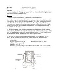
Introduction to Oscilloscope:
An oscilloscope is a versatile measurement tool that can display “real-time” plots of voltage versus time or
voltage versus voltage (in ‘X-Y’ mode). The vertical and horizontal axes of an oscilloscope can be
rescaled independently while data is being displayed. Unlike a graph that has a beginning and an end, an
oscilloscope’s plot of voltage (known as a “trace”) is refreshed or redrawn continuously as long as data is
being measured. One other difference is that an oscilloscope displays voltages, not calculated values
(e.g., velocity). An oscilloscope can be setup so that a plot of voltage will begin when a specific starting
condition (or “triggering” condition) occurs.
The oscilloscope allows the analysis of time-varying voltages over a wide dynamic range (frequency). Your
TA will explain the principle of operation. The signal trace is observed on a CRT (Cathode Ray Tube)
screen. The trace is produced by a beam of electrons swept across the phosphor screen by two sets of
electrostatic deflection plates. The trace is swept across the horizontal axis by the “Time Base” plates.
This sweep is regular and allows the divisions on the horizontal axis to be proportional to time. The trace is
swept in the vertical direction by the voltage input to the oscilloscope. The combination of these two
sweeps allows observation and analysis of time varying voltages. Since we are not using a “real
oscilloscope”, but adapting the computer to act as an oscilloscope the function is not quite the same. The
computer is acting more like a DMM, measuring voltage, but with time resolution,
(e.g. 5000 samples per second).
The Wave function Generator produces voltage waveforms that are regular in time. It can be used to
analyze a circuit’s response to a well defined input signal. The “response” of the circuit is the output signal,
which can be observed on an oscilloscope. Comparison of the input and output signal as a function of the
input frequency and amplitude, for example, can be an important diagnostic feature of a circuits’
performance.
Frequency and Period measurements:
The frequency of the wave output is the number of complete waves per second; units are in (cycles/second
or Hz). The PERIOD of the wave is the time taken for one complete cycle of a wave, (i.e., from one wave
crest to an adjacent wave crest).
The frequency (f) is equal to the inverse of the period (T), f = 1 / T.
Oscilloscope Procedure:
Note: If the Science Workshop Signal Interface was not turned on, the computer will ask you to try again
or continue w/o interface. If this happens check to make sure the interface is turned on and all connections
(Cables) are correct.
1) Turn on the computer, monitor, Science workshop interface and Pasco CI-6522 Power Amplifier II
2) Connect the voltage sensor (6500) to the signal interface II Analog channel A. Then connect the
Red lead to the Red terminal (Signal Output +) on the power amplifier II. Now connect the black
lead to the black terminal ( Signal output -) on the power amplifier II.
3) Connect the gray lead from the back of the amplifier II to the Signal Interface II Analog Channel B.
4) Now click the Data Studio icon on the desktop. A window will pop up in the data studio software
like the below one.
64

5) Click on the create experiment icon. A window like the one below will open.
6) Click on the yellow circle with Alphabet A over it. The following window will pop up.
65

7) Scroll the window until you reach the bottom of the window. Then click on the Voltage sensor and
click OK. The following window will open up.
8) Then click on the circular connector below the alphabet B. The following window will open up.
66

9) Scroll the window until you reach the Power Amplifier icon and click on it. Then click OK. The
following window will open up.
10) On the top field select the Sine Wave. In the amplitude field put 5 V. Then put 800 Hz in the
frequency field. Make sure that auto icon is clicked on.
11) On the main window of the data studio, at the left corner, you’ll see the following window.
12) Double click on the Scope icon. The following window will pop up.
67

13) Select Voltage, Output Voltage [V] and click OK. The following window will open up.
14) On the scope window set your voltage per division button to (A the only active-cell)
5.000v/div., (this is the small wave form button next to v/div.), and you time per division to
2.00 ms/div., (located at the bottom of the scope window, next to the trig button). The samples/sec
should be 5000.
15) Then click the start button on the top of the main window as shown below.
Click here
68

16) The sine wave will show up on the scope as shown below. The graph you’ll be seeing is the Voltage
vs Time graph, with voltage on the vertical axes and time on the horizontal axes. You can change
the settings for voltage and time on the scope by clicking on the arrows adjacent to the V/div and
ms/div.
17) Then click the stop button on the main window. For taking measurements, press XY button on the
Scope window, as shown above.
18) The following measurement tool will appear on the scope. You can use this to measure voltage and
time. You need to place the marker on the point you want to take the measurement.
19) Now click on the voltage per division’s button and change to 2v/div.,
(top button), and observe the change in the trace.
Question #1: What happened to the trace and why?
20) Use the x-y axis button (located below the trig button on the scope
window) to give a time display and a cross axis. Set the horizontal axis
at some fixed wave point then move the vertical axis from a point on one
wave to an adjacent point on the next wave point. Take the difference
of these two times and find the frequency. Make at least two measurements.
f= 1/T
21) Notice how the voltage reading changes as you move the horizontal
axis up and down. Click the x-y axis button again to turn it off or just
click the left mouse button.
22) Change time/div. scale from 2.00 ms/div. to 1.00 ms/div. (Right bottom) then to 0.50 ms/div.
Observe the change in the trace. Calculate the frequency. Did it change?
23) Click on stop Experiment.
24) Go to the Signal Generator window and change the Amplitude/Voltage to about 2.00 volts and the
frequency to 1200.00 Hz.
69

25) Go back to the Scope window and set voltage per divisions to 1.000v/div. and time scale to
0.20 ms/div. Make at least two measurements using the x-y axis button (as in described in step 20) at
This setting of 1200Hz. Calculate the frequency.
Oscilloscope table
Sample (no.) Initial time T 1 Final Time T 2 T= T 2 - T 1 Frequency (f) =
1/T
70

Name:
Lab Partners Name:
Lab Section:
Date of Experiment:
Format of Lab Reports and Grading
Title of the Experiment
(1 point for having a title)
Abstract (5): A concise statement (a paragraph or two) that summarizes the objective
and states the numerical results of the experiment, worth a total of 5 points.
1 point for having an abstract
2 points for summarizing objectives
2 points summarizing results
Theory (10): Summarize in your own words, the theory of the physics involved in the
experiment. Also present the working equations and the units. The theory sections should
also outline the procedures used in the lab, worth a total of 10 points.
5 points for having a theory section
2 points for outlining procedures
1 points for stating proper units
1 points for expressing relevant equations
1 points for defining relevant terms
Data (8): An orderly display of the data, preferably in tabular from. You must including
the original data sheet signed by the TA. All entries should be clearly identified and
include their proper units, worth a total of 8 points.
2 points for a data section
2 points original data (signed by instructor)
2 points for proper/clear labeling of data
2 points for proper units of data
Analysis (14): Must clearly show the computations used to reduce the data. First write
the relevant equations then give a sample calculation. Be sure to include
proper units and use the correct number of significant figures, worth a
total of 14 points.
2 points for having a computation section
2 points for displaying relevant formula
2 points for sample computation
2 points for proper units
2 points for significant figures
Graphs: 2 points proper units
2 points labeling axis
71

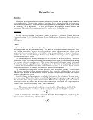
Results and conclusion (12):
A brief Summary of your results, stating the determined value or law,
along with its numerical uncertainty. Use proper units and significant
figures. For example, the experimental value for “g” was found to be:
Acceleration of gravity g = (9.8 0.2) m/s 2
Frequently you will want to compare your result (F) with an accepted value (F o ).
A good quantity to compute in this case is the “percent discrepancy” or the
“Percent error” which is defined as:
Percent
Discrepency
F
F
0
F
0
100%
If you are comparing two values of “F” found in different ways (F 1 and F 2 ) find
the “percent difference” given by:
Percent
Difference
F
F
1 2
F M
100%
Where F M is the mean of F 1 and F 2 . Round off percent errors and differences
to two significant figures. Discuss what you found and compare with what
you had expected to find. Discuss any discrepancies. One may suggest ways
in which to improve the experiment or reduce errors. Some labs may include
questions, worth a total of 12 points.
2 points for having a results section
2 points stating determined value
2 points for stating uncertainty
2 points for having a discussion section
2 points for summarizing experiment and results
2 points for each question answered correctly
Grade = (total points earned / total point available) X 100
72

Note: Your instructor will consider the above format important when grading
your lab report. The following may be taken into consideration as well. (Worth ≈ 10%)
1. Neatness
2. Composition
3. Grammar
4. Spelling
5. Thought and originality in performing and presenting the lab
6. Behavior that is disruptive to the labs (which includes but not limited to: being late to
class,
not leaving a clean work area for the following class…)
Bonus point will be given for finding and reporting errors in lab manual
Not all labs will conform exactly to the lab report format, given above.
Some labs may not require a certain section of the lab format. While another
lab may require an additional section be added to the write-up.
For nonconforming labs, check with the instructor as to what they expect
for a write up.
73