Teorema esantionarii Esantionarea ideala

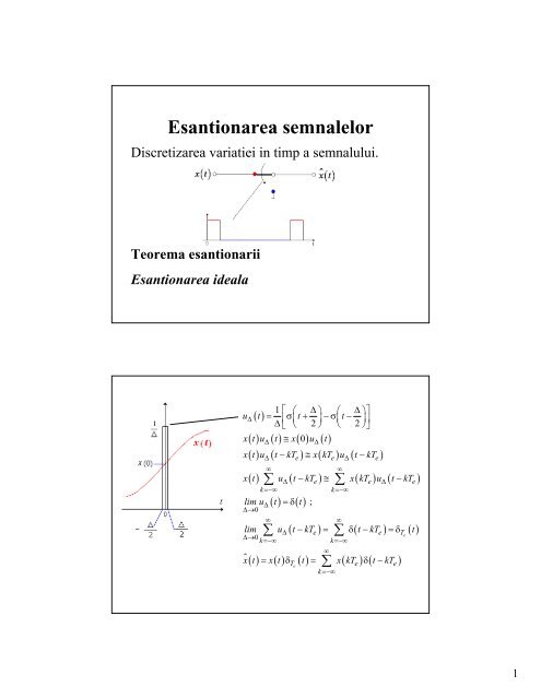
Esantionarea semnalelor
Discretizarea variatiei in timp a semnalului.
Teorema esantionarii
Esantionarea ideala
1 ⎡ ⎛ Δ⎞ ⎛ Δ⎞⎤
uΔ
() t = σ ⎜t+ ⎟−σ⎜t−
⎟
Δ
⎢
2 2
⎥
⎣ ⎝ ⎠ ⎝ ⎠⎦
xtu t x u t
() Δ() ≅ ( 0) Δ()
() ( − ) ≅ ( ) ( − )
xtu t kT xkT u t kT
Δ
∞
() ∑ Δ( − e) ≅ ∑ ( e) Δ( − e)
k=−∞
() =δ()
e e Δ e
x t u t kT x kT u t kT
lim u t t
Δ
Δ→0
∞
∑
( − e) = ∑ δ( − e) =δT
()
Δ
Δ→ 0
k =−∞ k =−∞
∞
;
xt $ () = xt () δ T () t = ∑ xkT ( e) δ( t−kTe)
e
k=−∞
k=−∞
lim u t kT t kT t
∞
∞
e
1

x $ () t = x() t δ () t = x( kT ) δ( t−kT
)
∞
∑
Te
e e
k=−∞
x(t)
x(t)= x(t)δ Te (t)
δ Te (t)
δ
Te
^
X
Spectrul semnalului esantionat
ideal
() t
1
{ } = X ( ω)
( ω) = F x() t δ () t
1
=
T
2π
↔
T
∞
∑
k =−∞
e
X
∞
∑
k =−∞
e
⎛ 2π
⎞ 2π
δ⎜ω − k ⎟ ; = ω
⎝ Te
⎠ Te
Te
⎛
2π
⎞
Te
⎠
∞
( ω) ∗δ⎜ω − k ⎟ = ∑
⎝
2π
2π
∗
T
1
T
k =−∞
e
e
∞
∑
k =−∞
e
⎛ 2π
⎞
δ⎜ω − k ⎟ =
⎝ Te
⎠
⎛ 2π
X ⎜ω − k
⎝ Te
⎞
⎟
⎠
2

^
X
1
T
( ω) = ∑ ∞
k −∞
e
⎛
⎜
⎝
2π
⎞
Te
⎠
X ω − k ⎟
=
Eroarea de aliere.
Teorema esantionarii semnalelor
de banda limitata
ω
ω
e
M
r
> 2ω
≤ ω
c
M
( 0) e
H = T
≤ ω
e
− ω
Nu apare aliere.
M
3

H
x
( ω) = T p ( ω)
() t = xˆ () t ∗ h () t ↔ X ( ω) = Xˆ ( ω) ⋅ H ( ω)
1
=
T
x
r
r
r
∑ ∞
k = −∞
e
X
() t = x() t , a.p.t
e
ωc
r
⎧Te
,
= ⎨
⎩ 0,
( ω − kω
) T p ( ω) = X ( ω)
e
e
r
ωc
ω ≤ ω
ω > ω
c
c
ω
M
,
≤ ω
r
c
≤ ω
=
e
− ω
M
ω
e
− ω
M
< ω
M
Apare alierea.
4

H
x
=
=
r
r
( ω) = T p ( ω) ↔ h ( t)
∞
c
() t = h () t ∗ xˆ () t = T ∗ ∑ x( kT ) δ( t − kT )
∞
∑
k =−∞
∞
∑
k =−∞
x
r
∞
c
( kT ) T ∗δ( t − kT ) = ∑ x( kT )
2ω
ω
e
c
devine: x
r
e
e
x
ωc
e
( kT )
e
c( t − kTe
)
( t − kT )
∞
() t = ∑ x( kT )
k =−∞
c
e
sinω
t
πt
sinω
ω
sinωct
r
= Te
πt
sinω
t
πt
k =−∞
e
e
M
e
sinω
ω
k =−∞
Frecventa de esantionare minima este ω
esantionarii la frecventa
M
( t − kTe
)
( t − kT )
e
e
e
e
= 2ω
M
e
=
sin
Te
π
ωc
( t − kTe
)
( t − kT )
denumirea de frecventa de esantionare Nyquist.In cazul
Nyquist formula de reconstructie
e
si poarta
=
Harry Nyquist , (February 7, 1889 – April 4, 1976)
was an important contributor to information theory.
He was born in Nilsby, Sweden. He emigrated to the
USA in 1907 and entered the University of North
Dakota in 1912. He received a Ph.D. in physics at
Yale University in 1917.
He worked at AT&T's Department of Development and Research from 1917 to
1934, and continued when it became Bell Telephone Laboratories in that year,
until his retirement in 1954. As an engineer at Bell Laboratories, he did
important work on thermal noise ("Johnson–Nyquist noise"), the stability of
feedback amplifiers, telegraphy, facsimile, television, and other
communications problems. In 1932, he published a classical paper on stability
of feedback amplifiers (H. Nyquist, "Regeneration theory", Bell System
Technical Journal, vol. 11, pp. 126-147, 1932). Nyquist stability criterion can
now be found in all textbooks on feedback control theory. His early theoretical
work on determining the bandwidth requirements for transmitting information,
as published in "Certain factors affecting telegraph speed" (Bell System
Technical Journal, 3, 324–346, 1924), laid the foundations for later advances by
Claude Shannon, which led to the development of information theory.
5

x
Teorema WKS (Whittaker,
Kotelnikov, Shannon)
x() t este de banda limitatala ωM
,in sensulca X ( ω)
ω > ωM
, atunci x()
t este unic determinatde multimea
{ x( nT ) n∈Z}
, daca ω ≥ 2ω
,
Daca semnalul
pentru
sale
putin dublulfrecventeimaxime.In conditiilede maisus semnalulinitial x
() t = x( kT )
e
∑ ∞
k = −∞
e
2ω
ω
c
e
c
sinω
ω
c
e
se poate reconstitui din esantioanele sale,a.p.t prin relatia:
c( t − kTe
)
( t − kT )
cu conditia ca ω sa fie astfelalesincat sa satisfaca relatia: ω
e
M
M
≤ ω
≡ 0
esantioanelor
adica frecventade esantionare este cel
c
≤ ω
e
() t
− ω
M
.
Edmund Taylor Whittaker Vladimir Kotelnikov Claude Shannon
Wikipedia
6

Edmund Whittaker was educated to Trinity College, Cambridge starting 1892.
After Whittaker became a Fellow of Trinity College he began to teach and give
lecture courses and, among his first pupils were G H Hardy and J H Jeans.
Whittaker made revolutionary changes to the topics taught at Cambridge. He
taught a course based on his famous book A Course of Modern Analysis
(1902). This work is important in the study of functions of a complex variable.
It also develops the theory of special functions and their related differential
equations. Other courses Whittaker taught at Cambridge included astronomy,
geometrical optics, and electricity and magnetism. Hardy and Jeans were not
the only famous mathematicians which Whitttaker taught at Cambridge.
His pupils included Bateman, Eddington, Littlewood, Turnbull,
and Watson. An application which interested him came through his association
with actuaries in Edinburgh who were dealing with life assurance. This motivated
him to study the mathematics lying behind somewhat ad hoc methods that the
actuaries were using and Whittaker proved some important results on interpolation
as a consequence.
Vladimir Aleksandrovich Kotelnikov (Russian, September 6, 1908 in Kazan –
February 11, 2005 in Moscow) was an information theory pioneer from the
Soviet Union. He was elected a member of the Russian Academy of Science, in
the Department of Technical Science (radio technology) in 1953.
• 1926-31 study of radio telecommunications at the Moscow Power Engineering
Institute, dissertation in engineering science.
• 1931-41 worked at the MEI as engineer, scientific assistant, laboratory director
and lecturer.
• 1941-44 worked as developer in the telecommunication industry.
• 1944-80 full professor at the MEI.
• 1953-87 deputy director and since 1954 director of the institute for radio
technology and electronics at the Russian Academy of Science.
• 1964 Lenin Prize
• 1970-88 vice-president of the RAS; since 1988 adviser of the presidium.
He is mostly known for having discovered, independently of others (e.g.
Edmund Whittaker, Harry Nyquist, Claude Shannon), the sampling theorem in
1933. This result of Fourier Analysis was known in harmonic analysis since the
end of the 19th century and circulated in the 1920s and 1930s in the engineering
community. He was the first to write down a precise statement of this theorem in
relation to signal transmission.
7

Shannon was born in Petoskey, Michigan. His childhood hero was Thomas
Edison, whom he later learned was a distant cousin. In 1932 he entered the
University of Michigan, where he took a course that introduced him to the
works of George Boole. He graduated in 1936 with two bachelor's degrees,
one in electrical engineering and one in mathematics, then began graduate
study at the Massachusetts Institute of Technology (MIT), where he worked
on Vannevar Bush's differential analyzer, an analog computer. A paper drawn
from his 1937 master's thesis, A Symbolic Analysis of Relay and Switching
Circuits, was published in the 1938 issue of the Transactions of the American
Institute of Electrical Engineers. Next, Shannon worked on his dissertation at
Cold Spring Harbor Laboratory, funded by the Carnegie Institution, to develop
similar mathematical relationships for Mendelian genetics, which resulted in
Shannon's 1940 PhD thesis at MIT, An Algebra for Theoretical Genetics.
Shannon then joined Bell Labs to work on fire-control systems and
cryptography during World War II, under a contract with section D-2 of the
National Defense Research Committee. In 1948 Shannon published A
Mathematical Theory of Communication, an article in two parts in the Bell
System Technical Journal. He is also credited with the introduction of
Sampling Theory.
He returned to MIT to hold an endowed chair in 1956.
Shannon and his famous electromechanical
mouse Theseus, named after the Greek
mythology hero of Minotaur and Labyrinth
fame, and which he tried to teach to come
out of the maze in one of the first
experiments in artificial intelligence.
Hobbies and inventions
Outside of his academic pursuits,
Shannon was interested in juggling,
unicycling, and chess. He also
invented many devices, including
rocket-powered flying discs, a
motorized pogo stick, and a flamethrowing
trumpet for a science
exhibition. One of his more
humorous devices was a box kept on
his desk called the "Ultimate
Machine“. Otherwise featureless, the
box possessed a single switch on its
side. When the switch was flipped,
the lid of the box opened and a
mechanical hand reached out, flipped
off the switch, then retracted back
inside the box.
8

Reconstructia prin filtrare trecejos
ideala
c ( − e)
( t kT )
ωc( e − e)
( nT kT )
∞
2ωc
sinω
t kT
x() t = ∑ x( kTe
)
k =−∞ ωe ωc − e
∞ 2ωc
sin nT kT
x( nTe) = ∑ x( kTe)
k =−∞ ωe ωc e − e
ωe
ω M = ⇒ ω MTe
= π
2
∞ sin π( n − k )
x( nTe) = ∑ x( kTe)
=
k =−∞ π( n − k)
∞
= ∑ x( kTe) δ n,k = x( nTe)
k =−∞
⎧1, n = k
δ n,k = ⎨
⎩0, n ≠ k
Tema de curs: Demonstrati ca relatia de reconstructie reprezinta o
descompunere a semnalului initial intr-o baza ortonormata a
spatiului semnalelor de energie finita si banda limitata.
Reconstructia prin interpolare
H
r
⎛ ωTe
⎞
⎜sin
T 2
⎟
ω = e⎜ ⎟
ωTe
⎜
⎟
⎝ 2 ⎠
( )
2
9

Reconstructia prin extrapolare
de ordinul zero
⎛ e ⎞
r()
= Te
⎜ −
2
⎟
⎝ ⎠
2
ωT
ωT
e
e
− j
2sin
e 2 2
ω
ωT
ωT
e
e
− j
sin
e 2 T 2
e
ωTe
2
ωTe
− j
( )
2
r
e
ω
ω sin π
−jπ ω ω e
h t p t
H ω = e T
ωTe
sin
2 =
ωTe
2
= e
e
e
T
↔ =
=
ω
π ω
10

Esantionarea ideala a
semnalelor periodice
2π
ω = Nω ; ω = ; ω = Mω
M
( )
0 0 e 0
T0
Pentru ca sa nu apara suprapunerea
lobilor centrali este necesar ca:
0 e 0 0
( )
( ) si
Nω ωc
Pentru a evita aparitia erorilor de aliere este necesar ca:
e
c
( ω ) = ω ( ω ) = ⎨
; Nω 0 2Nω = 2ω
e 0 0 e 0 M
Spre deosebire de semnalele aperiodice unde ω ≥2
ω
pentru semnalele periodice trebuie sa esantionam astfel incat
ω > 2 ω Pe perioada celei mai rapide componente spectrale
e M .
trebuie sa prelevam mai mult de doua esantioane (adica cel putin
3).
e
M
,
11

Daca T
0
este perioada fundamentalei si daca esantionarea se
2π
2π
face conform relatiei ω = 2 + ω atunci = 2 + ;
e
( ) ( )
N R 0
N R
Te
T 0
T0
R=1,2,...sau Te
=
2N
+ R
Doar 2 N+ R esantioane pot fi distincte ca urmare a periodicitatii
semnalului supus esantionarii. Toate pot fi prelevate
intr-o singura perioada a fundamentalei T .
0
Acelasi rezultat se poate obtine si preluand
esantioane succesive din perioade succesive.
( ) = ( + ) = ( + )
x kT x T kT x kT kT
e 0 e 0 e
T0
T' e = kT0 + Te
= kT0
+
2N
+ R
Aceasta posibilitate este valorificata in
constructia osciloscoapelor cu esantionare.
12

http://www.jhu.edu/~signals/sampling/index.html
Tema de curs: Folositi acest
applet pentru ca sa studiati
esantionarea unui semnal
sinusoidal.
0
2
Relatii energetice
Pentru semnale aperiodice esantionate este adevarata
relatia de tip Rayleigh:
∞
∫
() ( )
W = x t dt = T x kT
−∞
Pentru semnale periodice esantionate este valabila relatia
de tip Parseval:
1 2 1
∫
0 T
∞
∑
e
k=−∞
M −1
∑
() ( )
P= x t dt = x kTe
; M=2 N+ R, R=1,2,...
T
M
k=
0
e
2
Energia sau puterea pot fi calculate fie din forma de variatie in timp
fie in domeniul frecventa.
2
13

Esantionarea cu retinere
xt % () = ⎡xt () δ () t⎤∗ ht () = xt $ () ∗ht
()
⎣ T e ⎦
ωΔt
ωΔt
ωΔt
2
t
j
sin
ωΔ
j
sin
⎛ Δt
⎞ −
−
ht () = p 2 2 2 2
Δt
⎜t− ⎟↔ e = e Δt
⎝ 2 ⎠
ω
ωΔt
2
2
Spectrul semnalului esantionat
cu retinere
14

Acest caz se numeste
esantionare cu memorare.
Esantionarea naturala
x % () t = x() t qT () t = x() t ⎡h() t ∗δ T () t ⎤= ∑ x() t h( t− kTe) = ∑ x() t h( t−kTe)
e
⎛ Δt
⎞
unde ht p ⎜t ⎟ H e
⎝ 2 ⎠
() = − ↔ ( ω ) = 2
Δt
2
⎣
e
⎦
∞
k=−∞
jωΔt
−
ωΔt
2sin
2
ω
k=−∞
15

Spectrul semnalului esantionat
natural
16

Relatia dintre spectrul unui
semnal discret si spectrul
semnalului analogic din care
provine
17

Intre cele doua axe de frecventa corespunzatoare spectrului semnalului analogic esantionat respectiv
spectrului semnalului discret exista relatia: Ω=ωT. Se explica acum si natura periodica a spectrului
π
semnalului discret X d ( Ω)
. Intre ΩM si ωM exista relatia: Ω M =ωMTe ; T e ≤ . ω
e
M
18

Esantionarea semnalelor
discrete
In prelucrarea numerica a semnalelor apar situatii in care,
ulterior achizitionarii esantioanelor, se constata ca frecventa
de esantionare a fost prea mare. In astfel de situatii, cand nu
se mai poate esantiona semnalul analogic, este posibila
esantionarea semnalului numeric, retinandu-se tot a N-a valoare. Fie:
N
∞
[ n] ∑ [ n-kN]
δ = δ
k=−∞
$ [ ]
Semnalul discret esantionat, xn, se obtine prin produsul:
xn $ [ ] = xn [ ] δ N [ n] = xn [ ] ∑ δ[ n−kN]
∞
k=
−∞
∞
∑
k=−∞
[ ] [ ]
= xkNδ n−kN.
N=3.
19

N=3.
Cum Ω = T ω , unde ω este frecventa maxima din
[ ]
spectrul semnalului analogic din care provine xn,
iar T
e
M e M M
pasul cu care acest semnal analogic a fost
esantionat, rezulta:
π π
NT ≤ ; T ' ≤ ; T ' = NT
ω ω
e e e e
M
M
S-ar fi respectat teorema WKS chiar daca semnalul
() ar fi fost esantionat cu pasul Daca e
xt T'. Ω −Ω

Reconstruirea semnalului
discret din esantioanele sale
H
⎧N, Ω−2kπ ≤Ωc
Ω = ⎨
Ω ≤Ω ≤Ω −Ω
⎩ 0,
in rest
( )
r M c e M
.
Raspunsul la impuls al filtrului de reconstructie este:
h
r
r
[ n]
sin nΩc
Ωe
π
= ; Ω c = = .
nΩ
2 N
c
[ ] $ [ ] [ ] [ ]
x n = x n ∗ h n = x n ⇔
∞
[ ] = ∑
$ [ ] r [ − ]
xn xkh n k
k=−∞
r
xk $ [ ] = k≠ Nm xNm $ [ ] = xNm [ ]
Dar 0 pentru si si deci
⎛ π ⎞
∞
[ ] $ ∞ sin⎜
n −πm
⎟
N
xn= xNmh [ ] r [ n Nm] xNm
⎝ ⎠
∑
− = ∑ [ ]
π
m=−∞
m=−∞
n −π m
N
21

Esantionarea si decimarea unui
semnal discret
22

N=2.
23

Esantionarea spectrului unui
semnal discret de durata finita
24

[ ]
Fie xn cu suportul 0 ≤n≤M −1 . In urma esantionarii spectrului acestui semnal se obtine
% 2π
semnalul xn [ ] periodic de perioada N = . Daca N≥Mnu se produce suprapunerea
Ω
grupurilor temporale corespunzatoare diverselor valori k.
e
% ⎧2π
⎪ , 0≤n≤ N −1
Prin multiplicarea semnalului xn [ ] cu fereastra temporala rectangulara wr
[ n]
= ⎨ N
⎪⎩ 0,
in rest
[ ] , identic cu semnalul [ ] [ ] = [ ] = % [ ] [ ]
se obtine semnalul reconstruit x n x n : x n x n x n w n .
r r r
25

( )
Daca spectrul X Ω se esantioneaza prea rar, M < N, apare suprapunerea
grupurilor temporale, adica erori de tip "alias". Semnalul xn
fi reconstruit din spectrul esantionat.
[ ]
nu mai poate
Masuri practice la esantionarea
semnalelor analogice
De obicei nu se cunoaste largimea de banda a semnalului ce
urmeaza a fi esantionat. Acesta poate avea componente spectrale
de frecventa mare, neinteresante in aplicatia considerata.
Acestea pot fi de exemplu cauzate de zgomotul ce insoteste
semnalul util. Exista deci riscul aparitiei erorilor de tip "alias".
Pentru evitarea lor se prevede in structura lantului de prelucrare
a semnalului, inaintea circuitului de esantionare, un filtru trece jos
numit filtru "anti-alias" sau filtru de garda.
26

Esantionarea trebuie facuta cu
o frecventa de cel putin 2 ori
mai mare decat frecventa de
oprire ωs ωe ≥2ωs.
De asemenea trebuie sa avem
ωM
≤ωp.
Deci:
ωe
ωM ≤ω p

Semnal de vorbire fara aliasing.
Semnal de vorbire cu aliasing.
Semnal muzical fara aliasing.
Semnal muzical cu aliasing.
Esantionarea semnalelor trece
banda
Semnale de tip "trece jos" - spectrul concentrat in benzi care includ frecventa nula.
Semnale de tip "trece banda" - au suportul spectrului de forma [ −ωM , −ωm] ∪[ ωm, ωM
].
Reconstructia perfecta a unui semnal
trece banda esantionat ideal se poate
realiza pe baza teoremei WKS, ω e ≥ 2 ω M .
Uneori semnalele trece banda pot fi
reconstruite din esantioanele lor chiar daca
s-a folosit o frecventa de esantionare mai
mica decat frecventa Nyquist.
28

Cazul semnalelor trece banda
de banda ingusta
ωM
−ω m < 1.
ωm
Suportul spectrului unui semnal trece banda de banda ingusta
esantionat ideal este de forma:
supp X n , n n , n .
{ }
{ ( ω )} = U [ −ω + ω −ω + ω ] ∪[ ω + ω ω + ω ]
e M e m e m e M e
n∈Z
Semnalul trece banda de banda ingusta poate fi reconstruit
perfect din esantioanele sale chiar daca a fost folosita o
frecventa de esantionare mai mica decat frecventa Nyquist.
Conditia de reconstructie perfecta este:
[ −ω M + k ωe, −ω m + kωe] I [ ω m + l ωe, ω M + l ω e]
= ∅, ∀ k,
l∈
Z.
Pentru 0 conditia devine [ ] I [ ]
l = , −ω + k ω , −ω + k ω ω , ω =∅ ∀k∈Z.
M e m e m M
adica:
⎧ -ω
M + kωe ≤ωm 2ωM
2ωm
⎨ sau ≤ω e ≤ .
⎩ −ω M + ( k + 1)
ω e ≥ ω M k + 1 k
Daca exista valori intregi k, pentru care aceasta conditie este satisfacuta, atunci
exista valori ale frecventei de esantionare inferioare frecventei Nyquist pentru
care semnalele trece banda de banda ingusta pot fi reconstruite in urma
esantionarii ideale.
29

Solutia din multimea numerelor intregi a dublei inecuatii
ωm
obtinute este: 0 < k ≤ . Notand cu n0
partea intreaga
ω −ω
( )
a fractiei ω / ω −ω
M
m M m
m
, rezulta ca frecventa de esantionare
⎡2ωM
2ωm
⎤
va apartine unor intervale de forma ⎢ , cu k ∈{ 1,...,n 0 }.
k 1 k
⎥
⎣ + ⎦
Exemplu
ωm
ω m = 8 π si ω M = 10 π . Valoarea factorului n 0 este = 4.
ω −ω
Valorile admisibile pentru k sunt 1, 2, 3 si 4. Acestor valori le
corespund urmatoarele domenii pentru frecventa de esantionare:
{ 4π} U[ 5 π , 5,33π] U[ 6 66 π , 8π] U[ 10 π , 16π] U[
20 π , ∞]
, .
m
M
30