Special values of generalized log-sine integrals - CARMA ...
Special values of generalized log-sine integrals - CARMA ...
Special values of generalized log-sine integrals - CARMA ...

Create successful ePaper yourself
Turn your PDF publications into a flip-book with our unique Google optimized e-Paper software.
<strong>Special</strong> <strong>values</strong> <strong>of</strong> <strong>generalized</strong> <strong>log</strong>-<strong>sine</strong> <strong>integrals</strong><br />
Jonathan M. Borwein<br />
University <strong>of</strong> Newcastle<br />
Callaghan, NSW 2308, Australia<br />
jonathan.borwein@newcastle.edu.au<br />
Armin Straub<br />
Tulane University<br />
New Orleans, LA 70118, USA<br />
astraub@tulane.edu<br />
ABSTRACT<br />
We study <strong>generalized</strong> <strong>log</strong>-<strong>sine</strong> <strong>integrals</strong> at special <strong>values</strong>. At<br />
π and multiples there<strong>of</strong> explicit evaluations are obtained in<br />
terms <strong>of</strong> Nielsen poly<strong>log</strong>arithms at ±1. For general arguments<br />
we present algorithmic evaluations involving Nielsen<br />
poly<strong>log</strong>arithms at related arguments. In particular, we consider<br />
<strong>log</strong>-<strong>sine</strong> <strong>integrals</strong> at π/3 which evaluate in terms <strong>of</strong><br />
poly<strong>log</strong>arithms at the sixth root <strong>of</strong> unity. An implementation<br />
<strong>of</strong> our results for the computer algebra systems Mathematica<br />
and SAGE is provided.<br />
Keywords<br />
<strong>log</strong>-<strong>sine</strong> <strong>integrals</strong>, multiple poly<strong>log</strong>arithms, multiple zeta <strong>values</strong>,<br />
Clausen functions<br />
1. INTRODUCTION<br />
For n = 1, 2, . . . and k ≥ 0, we consider the (<strong>generalized</strong>)<br />
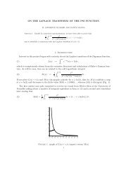
<strong>log</strong>-<strong>sine</strong> <strong>integrals</strong> defined by<br />
∫ σ<br />
∣ ∣∣∣<br />
Ls (k)<br />
n (σ) := − θ k <strong>log</strong> n−1−k 2 sin θ 2 ∣ dθ. (1)<br />
0<br />
The modulus is not needed for 0 ≤ σ ≤ 2π. For k = 0<br />
these are the (basic) <strong>log</strong>-<strong>sine</strong> <strong>integrals</strong> Ls n (σ) := Ls (0)<br />
n (σ).<br />
Various <strong>log</strong>-<strong>sine</strong> integral evaluations may be found in [20,<br />
§7.6 & §7.9].<br />
In this paper, we will be concerned with evaluations <strong>of</strong><br />
the <strong>log</strong>-<strong>sine</strong> <strong>integrals</strong> Ls n<br />
(k) (σ) for special <strong>values</strong> <strong>of</strong> σ. Such<br />
evaluations are useful for physics [15]: <strong>log</strong>-<strong>sine</strong> <strong>integrals</strong> appeared<br />
for instance in recent work on the ε-expansion <strong>of</strong><br />
various Feynman diagrams in the calculation <strong>of</strong> higher terms<br />
in the ε-expansion, [8, 16, 9, 11, 14]. Of particular importance<br />
are the <strong>log</strong>-<strong>sine</strong> <strong>integrals</strong> at the special <strong>values</strong> π/3,<br />
π/2, 2π/3, π. The <strong>log</strong>-<strong>sine</strong> <strong>integrals</strong> also appear in many<br />
settings in number theory and analysis: classes <strong>of</strong> inverse<br />
binomial sums can be expressed in terms <strong>of</strong> <strong>generalized</strong> <strong>log</strong><strong>sine</strong><br />
<strong>integrals</strong>, [10, 4].<br />
In Section 3 we focus on evaluations <strong>of</strong> <strong>log</strong>-<strong>sine</strong> and related<br />
<strong>integrals</strong> at π. General arguments are considered in Section<br />
Permission to make digital or hard copies <strong>of</strong> all or part <strong>of</strong> this work for<br />
personal or classroom use is granted without fee provided that copies are<br />
not made or distributed for pr<strong>of</strong>it or commercial advantage and that copies<br />
bear this notice and the full citation on the first page. To copy otherwise, to<br />
republish, to post on servers or to redistribute to lists, requires prior specific<br />
permission and/or a fee.<br />
Copyright 20XX ACM X-XXXXX-XX-X/XX/XX ...$10.00.<br />
5 with a focus on the case π/3 in Section 5.1. Imaginary<br />
arguments are briefly discussed in 5.2. The results obtained<br />
are suitable for implementation in a computer algebra system.<br />
Such an implementation is provided for Mathematica<br />
and SAGE, and is described in Section 7. This complements<br />
existing packages such as lsjk [15] for numerical evaluations<br />
<strong>of</strong> <strong>log</strong>-<strong>sine</strong> <strong>integrals</strong> or HPL [21] as well as [25] for working<br />
with multiple poly<strong>log</strong>arithms.<br />
Further motivation for such evaluations was sparked by<br />
our recent study [6] <strong>of</strong> certain multiple Mahler measures. For<br />
k functions (typically Laurent polynomials) in n variables<br />
the multiple Mahler measure µ(P 1, P 2, . . . , P k ), introduced<br />
in [18], is defined by<br />
∫ 1<br />
0<br />
∫ 1<br />
· · ·<br />
0<br />
k∏<br />
)∣<br />
∣<br />
<strong>log</strong> ∣P j<br />
(e 2πit 1 ∣∣<br />
, . . . , e 2πitn dt1dt 2 . . . dt n.<br />
j=1<br />
When P = P 1 = P 2 = · · · = P k this devolves to a higher<br />
Mahler measure, µ k (P ), as introduced and examined in [18].<br />
When k = 1 both reduce to the standard (<strong>log</strong>arithmic)<br />
Mahler measure [7].<br />
The multiple Mahler measure<br />
µ k (1+x+y ∗) := µ(1+x+y 1, 1+x+y 2, . . . , 1+x+y k ) (2)<br />
was studied by Sasaki [24, Lemma 1] who provided an evaluation<br />
<strong>of</strong> µ 2(1 + x + y ∗). It was observed in [6] that<br />
µ k (1 + x + y ∗) = 1 ( π<br />
)<br />
π Ls k+1 − 1 3 π Ls k+1 (π) . (3)<br />
Many other Mahler measures studied in [6, 1] were shown<br />
to have evaluations involving <strong>generalized</strong> <strong>log</strong>-<strong>sine</strong> <strong>integrals</strong><br />
at π and π/3 as well.<br />
To our knowledge, this is the most exacting such study<br />
undertaken — perhaps because it would be quite impossible<br />
without modern computational tools and absent a use <strong>of</strong> the<br />
quite recent understanding <strong>of</strong> multiple poly<strong>log</strong>arithms and<br />
multiple zeta <strong>values</strong> [3].<br />
2. PRELIMINARIES<br />
In the following, we will denote the multiple poly<strong>log</strong>arithm<br />
as studied for instance in [4] and [2, Ch. 3] by<br />
Li a1 ,...,a k<br />
(z) :=<br />
∑<br />
n a 1<br />
n 1 >···>n k >0<br />
z n 1<br />
1 · · · .<br />
na k<br />
For our purposes, the a 1, . . . , a k will usually be positive integers<br />
and a 1 ≥ 2 so that the sum converges for all |z| ≤ 1.<br />
For example, Li 2,1(z) = ∑ ∞ z k ∑ k−1 1<br />
k=1 k 2 j=1<br />
. In particular,<br />
j<br />
k
Li k (x) := ∑ ∞ x n<br />
n=1<br />
is the poly<strong>log</strong>arithm <strong>of</strong> order k. The<br />
n<br />
usual notation will k be used for repetitions so that, for instance,<br />
Li 2,{1} 3(z) = Li 2,1,1,1(z).<br />
Moreover, multiple zeta <strong>values</strong> are denoted by<br />
ζ(a 1, . . . , a k ) := Li a1 ,...,a k<br />
(1).<br />
Similarly, we consider the multiple Glaisher functions (Gl)<br />
and multiple Clausen functions (Cl) <strong>of</strong> depth k and weight<br />
w = a 1 + . . . + a k defined as<br />
{ }<br />
Im Lia1 ,...,a<br />
Cl a1 ,...,a k<br />
(θ) =<br />
k<br />
(e iθ ) if w even<br />
, (4)<br />
Re Li a1 ,...,a k<br />
(e iθ ) if w odd<br />
{<br />
Re Lia1 ,...,a<br />
Gl a1 ,...,a k<br />
(θ) =<br />
k<br />
(e iθ ) if w even<br />
Im Li a1 ,...,a k<br />
(e iθ ) if w odd<br />
}<br />
, (5)<br />
in accordance with [20]. Of particular importance will be<br />
the case <strong>of</strong> θ = π/3 which has also been considered in [4].<br />
Our other notation and usage is largely consistent with<br />
that in [20] and that in the newly published [23] in which<br />
most <strong>of</strong> the requisite material is described. Finally, a recent<br />
elaboration <strong>of</strong> what is meant when we speak about evaluations<br />
and “closed forms” is to be found in [5].<br />
3. EVALUATIONS AT π<br />
3.1 Basic <strong>log</strong>-<strong>sine</strong> <strong>integrals</strong> at π<br />
The exponential generating function, [19, 20],<br />
(<br />
− 1 ∞∑<br />
Ls m+1 (π) λm Γ (1 + λ)<br />
=<br />
π<br />
m! Γ ( ) =<br />
2 1 + λ 2<br />
m=0<br />
is well-known and implies the recurrence<br />
(−1) n<br />
n!<br />
Ls n+2 (π) = π α(n + 1)<br />
λ<br />
λ<br />
2<br />
)<br />
(6)<br />
n−2<br />
∑ (−1) k<br />
+<br />
(k + 1)! α(n − k) Ls k+2 (π) , (7)<br />
k=1<br />
where α(m) = (1 − 2 1−m )ζ(m).<br />
Example 1. (Values <strong>of</strong> Ls n (π)) We have Ls 2 (π) = 0 and<br />
− Ls 3 (π) = 1 12 π3<br />
Ls 4 (π) = 3 2 π ζ(3)<br />
− Ls 5 (π) = 19<br />
240 π5<br />
Ls 6 (π) = 45<br />
2 π ζ(5) + 5 4 π3 ζ(3)<br />
− Ls 7 (π) = 275<br />
1344 π7 + 45<br />
2 π ζ(3)2<br />
Ls 8 (π) = 2835<br />
4<br />
π ζ(7) + 315<br />
8 π3 ζ(5) + 133<br />
32 π5 ζ(3),<br />
and so forth. The fact that each integral is a multivariable<br />
rational polynomial in π and zeta-<strong>values</strong> follows directly<br />
from the recursion (7). Alternatively, these <strong>values</strong> may be<br />
conveniently obtained from (6) by a computer algebra system.<br />
For instance, in Mathematica the code<br />
FullSimplify[D[-Binomial[x,x/2], {x,6}] /.x->0]<br />
produces the above evaluation <strong>of</strong> Ls 6 (π).<br />
✸<br />
3.2 The <strong>log</strong>-<strong>sine</strong>-co<strong>sine</strong> <strong>integrals</strong><br />
The <strong>log</strong>-<strong>sine</strong>-co<strong>sine</strong> <strong>integrals</strong><br />
∫ σ<br />
∣ ∣∣∣<br />
Lsc m,n (σ) := − <strong>log</strong> m−1 2 sin θ ∣ ∣∣∣ 0<br />
2 ∣ <strong>log</strong>n−1 2 cos θ 2 ∣ dθ (8)<br />
appear in physical applications as well, see for instance [9,<br />
14]. They have also been considered by Lewin, [19, 20], and<br />
he demonstrates how their <strong>values</strong> at σ = π may be obtained<br />
much the same as those <strong>of</strong> the <strong>log</strong>-<strong>sine</strong> <strong>integrals</strong> in Section<br />
3.1. As observed in [1], Lewin’s result can be put in the form<br />
− 1 ∞∑<br />
Lsc m+1,n+1 (π) xm y n<br />
π<br />
m! n! = 2x+y Γ ( ) (<br />
1+x<br />
2 Γ 1+y<br />
)<br />
2<br />
π Γ ( )<br />
1 + x+y<br />
m,n=0<br />
2<br />
( )( ) ( ) ( )<br />
x y Γ 1 +<br />
x<br />
2 Γ 1 +<br />
y<br />
2<br />
=<br />
x/2 y/2 Γ ( )<br />
1 + x+y . (9)<br />
2<br />
The last form makes it clear that this is an extension <strong>of</strong> (6).<br />
The notation Lsc has been introduced in [9] where evaluations<br />
for other <strong>values</strong> <strong>of</strong> σ and low weight can be found.<br />
3.3 Log-<strong>sine</strong> <strong>integrals</strong> at π<br />
As Lewin [20, §7.9] sketches, at least for small <strong>values</strong> <strong>of</strong> n<br />
and k, the <strong>generalized</strong> <strong>log</strong>-<strong>sine</strong> <strong>integrals</strong> Ls (k)<br />
n (π) have closed<br />
forms involving ζ-<strong>values</strong> and Kummer-type constants such<br />
as Li 4(1/2). This will be made more precise in Remark 1.<br />
Our analysis starts with the generating function identity<br />
∫ π<br />
(<br />
2 sin θ ) λ<br />
e iµθ dθ<br />
2<br />
− ∑<br />
n,k≥0<br />
Ls (k) λn (iµ) k<br />
n+k+1<br />
(π) =<br />
n! k!<br />
= ie iπ λ (<br />
2 B1 µ −<br />
λ<br />
, 1 + λ) − ie iπµ (<br />
B<br />
2 1/2 µ −<br />
λ<br />
, −µ − )<br />
λ<br />
2 2<br />
(10)<br />
given in [20]. Here B x is the incomplete Beta function:<br />
B x(a, b) =<br />
∫ x<br />
0<br />
0<br />
t a−1 (1 − t) b−1 dt.<br />
We shall show that with care — because <strong>of</strong> the singularities<br />
at zero — (10) can be differentiated as needed as suggested<br />
by Lewin.<br />
Using the identities, valid for a, b > 0 and 0 < x < 1,<br />
( )<br />
B x(a, b) = xa (1 − x) b−1 1 − b, 1<br />
2F 1 x<br />
a<br />
a + 1 ∣ x − 1<br />
= xa (1 − x) b<br />
a<br />
2F 1<br />
( a + b, 1<br />
a + 1<br />
)<br />
∣ x ,<br />
found for instance in [23, §8.17(ii)], the generating function<br />
(10) can be rewritten as<br />
ie iπ λ 2<br />
(B 1<br />
(µ − λ )<br />
2 , 1 + λ − B −1<br />
(µ − λ ))<br />
2 , 1 + λ .<br />
Upon expanding this we obtain the following computationally<br />
more accessible generating function for Ls (k)<br />
n+k+1 (π):<br />
Theorem 1. For 2|µ| < λ < 1 we have<br />
− ∑<br />
Ls (k) λn (iµ) k<br />
n+k+1<br />
(π)<br />
n! k!<br />
n,k≥0<br />
= i ∑ ( )<br />
λ (−1) n e iπ λ 2 − e<br />
iπµ<br />
n µ − λ + n . (11)<br />
n≥0<br />
2
We now show how the <strong>log</strong>-<strong>sine</strong> <strong>integrals</strong> Ls n<br />
(k) (π) can quite<br />
comfortably be extracted from (11) by differentiating its<br />
right-hand side. The case n = 0 is covered by:<br />
Proposition 1. We have<br />
d k d m λ<br />
dµ k dλ i eiπ 2 − e<br />
iπµ<br />
∣<br />
m µ − λ 2<br />
∣ λ=0<br />
µ=0<br />
Pro<strong>of</strong>. This may be deduced from<br />
e x − e y<br />
x − y = ∑<br />
m,k≥0<br />
= ∑<br />
m,k≥0<br />
= π<br />
2 m (iπ)m+k B(m + 1, k + 1).<br />
x m y k<br />
(k + m + 1)!<br />
upon setting x = iπλ/2 and y = iπµ.<br />
B(m + 1, k + 1) xm y k<br />
m! k!<br />
The next proposition is most helpful in differentiation <strong>of</strong><br />
the right-hand side <strong>of</strong> (11) for n ≥ 1, Here, we denote a<br />
multiple harmonic number by<br />
H [α]<br />
n−1 :=<br />
If α = 0 we set H [0]<br />
n−1 := 1.<br />
∑ 1<br />
. (12)<br />
i<br />
n>i 1 >i 2 >...>i α<br />
1i 2 · · · i α<br />
Proposition 2. For n ≥ 1<br />
( ) ( )<br />
(−1) α α ∣∣∣∣λ=0<br />
d λ<br />
= (−1)n<br />
α! dλ n<br />
n<br />
Note that, for α ≥ 0,<br />
∑<br />
n≥0<br />
(±1) n<br />
H [α]<br />
n β n−1 = Li β,{1} α(±1)<br />
H [α−1]<br />
n−1 . (13)<br />
which shows that the evaluation <strong>of</strong> the <strong>log</strong>-<strong>sine</strong> <strong>integrals</strong> will<br />
involve Nielsen poly<strong>log</strong>arithms at ±1, that is poly<strong>log</strong>arithms<br />
<strong>of</strong> the type Li a,{1} b(±1).<br />
Using the Leibniz rule coupled with Proposition 2 to differentiate<br />
(11) for n ≥ 1 and Proposition 1 in the case n = 0,<br />
(π) as a finite sum <strong>of</strong><br />
Nielsen poly<strong>log</strong>arithms with coefficients only being rational<br />
multiples <strong>of</strong> powers <strong>of</strong> π. The process is now exemplified for<br />
it is possible to explicitly write Ls (k)<br />
n<br />
Ls (2)<br />
4 (π) and Ls (1)<br />
5 (π).<br />
Example 2. (Ls (2)<br />
4 (π)) To find Ls (2)<br />
4 (π) we differentiate<br />
(11) once with respect to λ and twice with respect to µ. To<br />
simplify computation, we exploit the fact that the result will<br />
be real which allows us to neglect imaginary parts:<br />
− Ls (2)<br />
4 (π) = d2<br />
dµ 2 d<br />
dλ i ∑ n≥0<br />
= 2π ∑ n≥1<br />
(<br />
λ<br />
n<br />
)<br />
(−1) n e iπ λ 2<br />
(−1) n+1<br />
= 3 2 πζ(3).<br />
n 3<br />
− e<br />
iπµ<br />
µ − λ 2 + n ∣<br />
∣∣∣λ=µ=0<br />
In the second step we were able to drop the term corresponding<br />
to n = 0 because its contribution −iπ 4 /24 is purely<br />
imaginary as follows a priori from Proposition 2. ✸<br />
Example 3. (Ls (1)<br />
5 (π)) Similarly, setting<br />
Li ± a 1 ,...,a n<br />
:= Li a1 ,...,a n<br />
(1) − Li a1 ,...,a n<br />
(−1)<br />
we obtain Ls (1)<br />
5 (π) as<br />
− Ls (1)<br />
5 (π) = 3 4<br />
∑<br />
n≥1<br />
8(1 − (−1) n )<br />
(<br />
)<br />
nH [2]<br />
n 4 n−1 − Hn−1<br />
+ 6(1 − (−1)n )<br />
n 5<br />
− π2<br />
n 3<br />
= 6 Li ± 3,1,1 −6 Li ± 4,1 + 9 2 Li± 5 − 3 4 π2 ζ(3)<br />
= − 6 Li 3,1,1(−1) + 105<br />
32 ζ(5) − 1 4 π2 ζ(3).<br />
The last form is what is automatically produced by our program,<br />
see Example 13, and is obtained from the previous<br />
expression by reducing the poly<strong>log</strong>arithms as discussed in<br />
Section 6.<br />
✸<br />
The next example hints at the rapidly growing complexity<br />
<strong>of</strong> these <strong>integrals</strong>, especially when compared to the evaluations<br />
given in Examples 2 and 3.<br />
Example 4. (Ls (1)<br />
6 (π)) Proceeding as before we find<br />
− Ls (1)<br />
6 (π) = − 24 Li ± 3,1,1,1 +24 Li ± 4,1,1 −18 Li ± 5,1 +12 Li ± 6<br />
+ 3π 2 ζ(3, 1) − 3π 2 ζ(4) + π6<br />
480<br />
= 24 Li 3,1,1,1(−1) − 18 Li 5,1(−1)<br />
+ 3ζ(3) 2 − 3<br />
1120 π6 . (14)<br />
In the first equality, the term π 6 /480 is the one corresponding<br />
to n = 0 in (11) obtained from Proposition 1. The<br />
second form is again the automatically reduced output <strong>of</strong><br />
our program.<br />
✸<br />
Remark 1. From the form <strong>of</strong> (11) and (13) we find that<br />
the <strong>log</strong>-<strong>sine</strong> <strong>integrals</strong> Ls (k)<br />
n (π) can be expressed in terms <strong>of</strong> π<br />
and Nielsen poly<strong>log</strong>arithms at ±1. Using the duality results<br />
in [3, §6.3, and Example 2.4] the poly<strong>log</strong>arithms at −1 may<br />
be explicitly reexpressed as multiple poly<strong>log</strong>arithms at 1/2.<br />
Some examples are given in [6].<br />
Particular cases <strong>of</strong> Theorem 1 have been considered in<br />
[15] where explicit formulae are given for Ls (k)<br />
n (π) where<br />
k = 0, 1, 2.<br />
✸<br />
=<br />
Remark 2. A real form <strong>of</strong> Theorem 1 is the following:<br />
∫ π<br />
(<br />
2 sin θ ) x<br />
e θy dθ<br />
2<br />
0<br />
∞∑<br />
n=0<br />
(−1) n( ) ( (<br />
x<br />
n y (−1) n ) ( ) )<br />
e πy − cos πx<br />
2 − n −<br />
x<br />
2 sin<br />
πx<br />
2<br />
( )<br />
n −<br />
x 2<br />
.<br />
+ y<br />
2<br />
2<br />
From here, one may now also adduce one-variable generating<br />
functions. For instance,<br />
∞∑<br />
∞<br />
( )<br />
Ls (1) λn<br />
n+2 (π)<br />
n! = ∑ λ (−1) n cos πλ<br />
2<br />
( ) − 1<br />
n<br />
n=0<br />
n=0 n −<br />
λ 2<br />
, (15)<br />
2<br />
and we may again extract individual <strong>values</strong>.<br />
✸
3.4 Log-<strong>sine</strong> <strong>integrals</strong> at 2π<br />
As observed by Lewin [20, 7.9.8], <strong>log</strong>-<strong>sine</strong> <strong>integrals</strong> at 2π<br />
are expressible in terms <strong>of</strong> zeta <strong>values</strong> only. If we proceed<br />
as in the case <strong>of</strong> evaluations at π in (10) we find that the resulting<br />
integral now becomes expressible in terms <strong>of</strong> gamma<br />
functions:<br />
− ∑<br />
n,k≥0<br />
Ls (k) λn (iµ) k<br />
n+k+1<br />
(2π) =<br />
n! k!<br />
∫ 2π<br />
0<br />
(<br />
2 sin θ 2<br />
) λ<br />
e iµθ dθ<br />
( )<br />
= 2πe iµπ λ<br />
λ<br />
+ µ 2<br />
(16)<br />
The special case µ = 0, in the light <strong>of</strong> (21) which gives<br />
Ls n (2π) = 2 Ls n (π), recovers (6).<br />
We may now extract <strong>log</strong>-<strong>sine</strong> <strong>integrals</strong> Ls n<br />
(k) (2π) in a similar<br />
way as described in Section 3.1.<br />
Example 5. For instance,<br />
Ls (2)<br />
5 (2π) = − 13<br />
45 π5 .<br />
We remark that this evaluation is incorrectly given in [20,<br />
(7.144)] as 7π 5 /30 underscoring an advantage <strong>of</strong> automated<br />
evaluations over tables (indeed, there are more misprints in<br />
[20] pointed out for instance in [9, 15]). ✸<br />
3.5 Log-<strong>sine</strong>-poly<strong>log</strong> <strong>integrals</strong><br />
Motivated by the <strong>integrals</strong> LsLsc k,i,j defined in [14] we<br />
show that the considerations <strong>of</strong> Section 3.3 can be extended<br />
to more involved <strong>integrals</strong> including<br />
∫ π<br />
(<br />
Ls (k)<br />
n (π; d) := − θ k <strong>log</strong> n−k−1 2 sin θ )<br />
Li d (e iθ ) dθ.<br />
2<br />
0<br />
On expressing Li d (e iθ ) as a series, rearranging, and applying<br />
Theorem 1, we obtain the following exponential generating<br />
function for Ls (k)<br />
n (π; d):<br />
Corollary 1. For d ≥ 0 we have<br />
where<br />
− ∑<br />
n,k≥0<br />
Ls (k) λn (iµ) k<br />
n+k+1<br />
(π; d)<br />
n! k!<br />
= i ∑ λ H n,d (λ) eiπ 2 − (−1) n e iπµ<br />
µ − λ + n (17)<br />
n≥1<br />
2<br />
H n,d (λ) :=<br />
n−1<br />
∑<br />
k=0<br />
(−1) k( )<br />
λ<br />
k<br />
(n − k) . (18)<br />
d<br />
We note for 0 ≤ θ ≤ π that Li −1(e iθ ) = −1/ ( ) 2,<br />
2 sin θ 2<br />
Li 0(e iθ ) = − 1 + i cot θ , while 2 2 2 Li1(eiθ ) = − <strong>log</strong> ( )<br />
2 sin θ 2 +<br />
i π−θ , and (<br />
2 Li2(eiθ ) = ζ(2) + θ θ − π) + i Cl<br />
2 2 2 (θ).<br />
Remark 3. Corresponding results for an arbitrary Dirichlet<br />
series L a,d (x) := ∑ n≥1 anxn /n d can be easily derived in<br />
the same fashion. Indeed, for<br />
Ls (k)<br />
n (π; a, d) := −<br />
∫ π<br />
0<br />
θ k <strong>log</strong> n−k−1 (<br />
2 sin θ 2<br />
)<br />
L a,d (e iθ ) dθ<br />
one derives the exponential generating function (17) with<br />
H n,d (λ) replaced by<br />
H n,a,d (λ) :=<br />
n−1<br />
∑<br />
k=0<br />
(−1) k( λ<br />
k)<br />
an−k<br />
(n − k) d . (19)<br />
This allows for Ls (k)<br />
n (π; a, d) to be extracted for many number<br />
theoretic functions. It does not however seem to cover<br />
any <strong>of</strong> the <strong>values</strong> <strong>of</strong> the LsLsc k,i,j function defined in [14]<br />
that are not already covered by Corollary 1.<br />
✸<br />
4. QUASIPERIODIC PROPERTIES<br />
As shown in [20, (7.1.24)], it follows from the periodicity<br />
<strong>of</strong> the integrand that, for integers m,<br />
Ls (k)<br />
n<br />
(2mπ) − Ls (k)<br />
n (2mπ − σ)<br />
( )<br />
k∑<br />
= (−1) k−j (2mπ) j k<br />
j<br />
j=0<br />
Ls (k−j)<br />
n−j (σ) . (20)<br />
Based on this quasiperiodic property <strong>of</strong> the <strong>log</strong>-<strong>sine</strong> <strong>integrals</strong>,<br />
the results <strong>of</strong> Section 3.4 easily generalize to show<br />
that <strong>log</strong>-<strong>sine</strong> <strong>integrals</strong> at multiples <strong>of</strong> 2π evaluate in terms<br />
<strong>of</strong> zeta <strong>values</strong>. This is shown in Section 4.1. It then follows<br />
from (20) that <strong>log</strong>-<strong>sine</strong> <strong>integrals</strong> at general arguments can<br />
be reduced to <strong>log</strong>-<strong>sine</strong> <strong>integrals</strong> at arguments 0 ≤ σ ≤ π.<br />
This is discussed briefly in Section 4.2.<br />
Example 6. In the case k = 0, we have that<br />
Ls n (2mπ) = 2m Ls n (π) . (21)<br />
For k = 1, specializing (20) to σ = 2mπ then yields<br />
as is given in [20, (7.1.23)].<br />
Ls (1)<br />
n (2mπ) = 2m 2 π Ls n−1 (π)<br />
4.1 Log-<strong>sine</strong> <strong>integrals</strong> at multiples <strong>of</strong> 2π<br />
For odd k, specializing (20) to σ = 2mπ, we find<br />
( )<br />
k∑<br />
2 Ls (k)<br />
n (2mπ) = (−1) j−1 (2mπ) j k<br />
Ls (k−j)<br />
n−j (2mπ)<br />
j<br />
j=1<br />
giving Ls (k)<br />
n (2mπ) in terms <strong>of</strong> lower order <strong>log</strong>-<strong>sine</strong> <strong>integrals</strong>.<br />
More generally, on setting σ = 2π in (20) and summing<br />
the resulting equations for increasing m in a telescoping fashion,<br />
we arrive at the following reduction. We will use the<br />
standard notation<br />
H (a)<br />
n :=<br />
for <strong>generalized</strong> harmonic sums.<br />
n∑<br />
k=1<br />
k −a<br />
Theorem 2. For integers m ≥ 0,<br />
( )<br />
k∑<br />
Ls (k)<br />
n (2mπ) = (−1) k−j (2π) j k<br />
H m<br />
(−j) Ls (k−j)<br />
n−j (2π) .<br />
j<br />
j=0<br />
Summarizing, we have thus shown that the <strong>generalized</strong><br />
<strong>log</strong>-<strong>sine</strong> <strong>integrals</strong> at multiples <strong>of</strong> 2π may always be evaluated<br />
in terms <strong>of</strong> <strong>integrals</strong> at 2π. In particular, Ls (k)<br />
n (2mπ) can<br />
always be evaluated in terms <strong>of</strong> zeta <strong>values</strong> by the methods<br />
<strong>of</strong> Section 3.4.<br />
✸
4.2 Reduction <strong>of</strong> arguments<br />
A general (real) argument σ can be written uniquely as<br />
σ = 2mπ ± σ 0 where m ≥ 0 is an integer and 0 ≤ σ 0 ≤ π.<br />
It then follows from (20) and<br />
Ls (k)<br />
n<br />
that Ls (k)<br />
n (σ) equals<br />
Ls (k)<br />
n (2mπ) ±<br />
(−θ) = (−1) k+1 Ls n<br />
(k) (θ)<br />
( )<br />
k∑<br />
(±1) k−j (2mπ) j k<br />
j<br />
j=0<br />
Ls (k−j)<br />
n−j (σ 0) . (22)<br />
Since the evaluation <strong>of</strong> <strong>log</strong>-<strong>sine</strong> <strong>integrals</strong> at multiples <strong>of</strong> 2π<br />
was explicitly treated in Section 4.1 this implies that the<br />
evaluation <strong>of</strong> <strong>log</strong>-<strong>sine</strong> <strong>integrals</strong> at general arguments σ reduces<br />
to the case <strong>of</strong> arguments 0 ≤ σ ≤ π.<br />
5. EVALUATIONS AT OTHER VALUES<br />
In this section we first discuss a method for evaluating<br />
the <strong>generalized</strong> <strong>log</strong>-<strong>sine</strong> <strong>integrals</strong> at arbitrary arguments in<br />
terms <strong>of</strong> Nielsen poly<strong>log</strong>arithms at related arguments. The<br />
gist <strong>of</strong> our technique originates with Fuchs ([12], [20, §7.10]).<br />
Related evaluations appear in [8] for Ls 3 (τ) to Ls 6 (τ) as well<br />
as in [9] for Ls n (τ) and Ls (1)<br />
n (τ).<br />
We then specialize to evaluations at π/3 in Section 5.1.<br />
The poly<strong>log</strong>arithms arising in this case have been studied<br />
under the name <strong>of</strong> multiple Clausen and Glaisher <strong>values</strong> in<br />
[4]. In fact, the next result (23) with τ = π/3 is a modified<br />
version <strong>of</strong> [4, Lemma 3.2]. We employ the notation<br />
(<br />
)<br />
n<br />
:=<br />
a 1, . . . , a k<br />
for multinomial coefficients.<br />
n!<br />
a 1! · · · a k !(n − a 1 − . . . − a k )!<br />
Theorem 3. For 0 ≤ τ ≤ 2π, and nonnegative integers<br />
n, k such that n − k ≥ 2,<br />
k∑<br />
ζ(n − k, {1} k (−iτ) j<br />
) −<br />
Li<br />
j! 2+k−j,{1} n−k−2(e iτ )<br />
j=0<br />
(<br />
)<br />
= ik+1 (−1) n−1 n−k−1<br />
∑ r∑ n − 1<br />
(n − 1)!<br />
k, m, r − m<br />
r=0 m=0<br />
( ) r i<br />
× (−π) r−m Ls (k+m)<br />
n−(r−m)<br />
(τ) . (23)<br />
2<br />
Pro<strong>of</strong>. Starting with<br />
Li k,{1} n(α) − Li k,{1} n(1) =<br />
∫ α<br />
1<br />
Li k−1,{1} n(z)<br />
z<br />
and integrating by parts repeatedly, we obtain<br />
k−2<br />
∑ (−1) j<br />
<strong>log</strong> j (α) Li k−j,{1} n(α) − Li k,{1} n(1)<br />
j!<br />
j=0<br />
∫ α<br />
= (−1)k−2 <strong>log</strong> k−2 (z) Li {1} n+1(z)<br />
dz. (24)<br />
(k − 2)! 1<br />
z<br />
Letting α = e iτ and changing variables to z = e iθ , as well<br />
as using<br />
Li {1} n(z) =<br />
(− <strong>log</strong>(1 − z))n<br />
,<br />
n!<br />
dz<br />
the right-hand side <strong>of</strong> (24) can be rewritten as<br />
(−1) k−2 i<br />
(k − 2)! (n + 1)!<br />
∫ τ<br />
0<br />
( (<br />
(iθ) k−2 − <strong>log</strong> 1 − e iθ)) n+1<br />
dθ.<br />
Since, for 0 ≤ θ ≤ 2π and the principal branch <strong>of</strong> the <strong>log</strong>arithm,<br />
<strong>log</strong>(1 − e iθ ) = <strong>log</strong><br />
∣ 2 sin θ 2 ∣ + i (θ − π), (25)<br />
2<br />
this last integral can now be expanded in terms <strong>of</strong> <strong>generalized</strong><br />
<strong>log</strong>-<strong>sine</strong> <strong>integrals</strong> at τ.<br />
k−2<br />
∑<br />
ζ(k, {1} n ) −<br />
(−iτ) j<br />
Li k−j,{1} n(e iτ )<br />
j!<br />
j=0<br />
(<br />
= (−i)k−1 (−1) n n+1<br />
∑ r∑<br />
(k − 2)! (n + 1)!<br />
r=0 m=0<br />
( i<br />
2<br />
n + 1<br />
r<br />
)(<br />
)<br />
r<br />
m<br />
) r<br />
(−π) r−m Ls (k+m−2)<br />
n+k−(r−m)<br />
(τ) . (26)<br />
Applying the MZV duality formula [3], we have<br />
ζ(k, {1} n ) = ζ(n + 2, {1} k−2 ),<br />
and a change <strong>of</strong> variables yields the claim.<br />
We recall that the real and imaginary parts <strong>of</strong> the multiple<br />
poly<strong>log</strong>arithms are Clausen and Glaisher functions as<br />
defined in (4) and (5).<br />
Example 7. Applying (23) with n = 4 and k = 1 and<br />
solving for Ls (1)<br />
4 (τ) yields<br />
Ls (1)<br />
4 (τ) = 2ζ(3, 1) − 2 Gl 3,1 (τ) − 2τ Gl 2,1 (τ)<br />
+ 1 4 Ls(3) 4 (τ) − 1 2 π Ls(2) 3 (τ) + 1 4 π2 Ls (1)<br />
2 (τ)<br />
= 1<br />
180 π4 − 2 Gl 3,1 (τ) − 2τ Gl 2,1 (τ)<br />
− 1 16 τ 4 + 1 6 πτ 3 − 1 8 π2 τ 2 .<br />
For the last equality we used the trivial evaluation<br />
Ls (n−1)<br />
n (τ) = − τ n n . (27)<br />
It appears that both Gl 2,1 (τ) and Gl 3,1 (τ) are not reducible<br />
for τ = π/2 or τ = 2π/3. Here, reducible means expressible<br />
in terms <strong>of</strong> multi zeta <strong>values</strong> and Glaisher functions <strong>of</strong><br />
the same argument and lower weight. In the case τ = π/3<br />
such reductions are possible. This is discussed in Example 9<br />
and illustrates how much less simple <strong>values</strong> at 2π/3 are than<br />
those at π/3. We remark, however, that Gl 2,1 (2π/3) is reducible<br />
to one-dimensional poly<strong>log</strong>arithmic terms [6]. In [1]<br />
explicit reductions for all weight four or less poly<strong>log</strong>arithms<br />
are given.<br />
✸<br />
Remark 4. Lewin [20, 7.4.3] uses the special case k = n −<br />
2 <strong>of</strong> (23) to deduce a few small integer evaluations <strong>of</strong> the<br />
<strong>log</strong>-<strong>sine</strong> <strong>integrals</strong> Ls n<br />
(n−2) (π/3) in terms <strong>of</strong> classical Clausen<br />
functions.<br />
✸<br />
In general, we can use (23) recursively to express the<br />
<strong>log</strong>-<strong>sine</strong> <strong>values</strong> Ls (k)<br />
n (τ) in terms <strong>of</strong> multiple Clausen and<br />
Glaisher functions at τ.
Example 8. (23) with n = 5 and k = 1 produces<br />
Ls (1)<br />
5 (τ) = −6ζ(4, 1) + 6 Cl 3,1,1 (τ) + 6τ Cl 2,1,1 (τ)<br />
+ 3 4 Ls(3) 5 (τ) − 3 2 π Ls(2) 4 (τ) + 3 4 π2 Ls (1)<br />
3 (τ) .<br />
Applying (23) three more times to rewrite the remaining <strong>log</strong><strong>sine</strong><br />
<strong>integrals</strong> produces an evaluation <strong>of</strong> Ls (1)<br />
5 (τ) in terms <strong>of</strong><br />
multi zeta <strong>values</strong> and Clausen functions at τ.<br />
✸<br />
5.1 Log-<strong>sine</strong> <strong>integrals</strong> at π/3<br />
We now apply the general results obtained in Section 5<br />
to the evaluation <strong>of</strong> <strong>log</strong>-<strong>sine</strong> <strong>integrals</strong> at τ = π/3. Accordingly,<br />
we encounter multiple poly<strong>log</strong>arithms at the basic 6-<br />
th root <strong>of</strong> unity ω := exp(iπ/3). Their real and imaginary<br />
parts satisfy various relations and reductions, studied in [4],<br />
which allow us to further treat the resulting evaluations. In<br />
general, these poly<strong>log</strong>arithms are more tractable than those<br />
at other <strong>values</strong> because ω = ω 2 .<br />
Example 9. (Values at π ) Continuing Example 7 we have<br />
3<br />
(<br />
− Ls (1) π<br />
) ( π<br />
)<br />
4 = 2 Gl 3,1 + 2 ( π<br />
)<br />
3 3 3 π Gl2,1 + 19<br />
3 6480 π4 .<br />
Using known reductions from [4] we get:<br />
( π<br />
)<br />
Gl 2,1 = 1<br />
( π<br />
)<br />
3 324 π3 , Gl 3,1 = − 23<br />
3 19440 π4 , (28)<br />
and so arrive at<br />
(<br />
− Ls (1) π<br />
)<br />
4 = 17<br />
3 6480 π4 . (29)<br />
Lewin explicitly mentions (29) in the preface to [20] because<br />
<strong>of</strong> its “queer” nature which he compares to some <strong>of</strong> Landen’s<br />
curious 18th century formulas.<br />
✸<br />
Many more reduction besides (28) are known. In particular,<br />
the one-dimensional Glaisher and Clausen functions<br />
reduce as follows [20]:<br />
Gl n (2πx) = 2n−1 (−1) 1+⌊n/2⌋<br />
B n(x) π n ,<br />
n!<br />
( π<br />
)<br />
Cl 2n+1 = 1 3 2 (1 − 2−2n )(1 − 3 −2n )ζ(2n + 1). (30)<br />
Here, B n denotes the n-th Bernoulli polynomial. Further<br />
reductions can be derived for instance from the duality result<br />
[4, Theorem 4.4]. For low dimensions, we have built these<br />
reductions into our program, see Section 6.<br />
Example 10. (Values <strong>of</strong> Ls n (π/3)) The <strong>log</strong>-<strong>sine</strong> <strong>integrals</strong><br />
at π/3 are evaluated by our program as follows:<br />
( π<br />
) ( π<br />
)<br />
Ls 2 = Cl 2<br />
3 3<br />
( π<br />
)<br />
− Ls 3 = 7<br />
3 108 π3<br />
( π<br />
)<br />
Ls 4 = 1 3 2 π ζ(3) + 9 ( π<br />
)<br />
2 Cl4 3<br />
( π<br />
)<br />
− Ls 5 = 1543<br />
( π<br />
)<br />
3 19440 π5 − 6 Gl 4,1<br />
3<br />
( π<br />
)<br />
Ls 6 = 15 35<br />
π ζ(5) +<br />
3 2 36 π3 ζ(3) + 135 ( π<br />
)<br />
2 Cl6 3<br />
( π<br />
)<br />
− Ls 7 = 74369<br />
3 326592 π7 + 15<br />
( π<br />
)<br />
2 πζ(3)2 − 135 Gl 6,1<br />
3<br />
As follows from the results <strong>of</strong> Section 5 each integral is a<br />
multivariable rational polynomial in π as well as Cl, Gl,<br />
and ζ-<strong>values</strong>. These evaluations ( confirm those given in [9,<br />
Appendix A] for Ls π<br />
) (<br />
3 3 , π<br />
) (<br />
Ls4<br />
3 , and π<br />
)<br />
Ls6<br />
3 . Less explicitely,<br />
the evaluations <strong>of</strong> Ls π<br />
( ) (<br />
5 3 and π<br />
)<br />
Ls7<br />
3 can be recovered<br />
from similar results in [15, 9] (which in part were<br />
obtained using PSLQ; we refer to Section 6 for how our<br />
analysis relies on PSLQ).<br />
The first presumed-irreducible value that occurs is<br />
( π<br />
) ∑ ∞∑ n−1 1 (<br />
k=1 k nπ<br />
)<br />
Gl 4,1 =<br />
sin<br />
3<br />
n 4 3<br />
n=1<br />
= 3341<br />
1632960 π5 − 1 π ζ(3)2 − 3<br />
4π<br />
∞∑<br />
n=1<br />
1<br />
( 2n<br />
n<br />
)<br />
n<br />
6 . (31)<br />
The final evaluation is described in [4]. Extensive computation<br />
suggests it is not expressible as a sum <strong>of</strong> products <strong>of</strong><br />
one dimensional ζ-<strong>values</strong>. Indeed, conjectures are made in<br />
[4, §5] for the number <strong>of</strong> irreducibles at each depth. Related<br />
dimensional conjectures for poly<strong>log</strong>s are discussed in [26]. ✸<br />
5.2 Log-<strong>sine</strong> <strong>integrals</strong> at imaginary <strong>values</strong><br />
The approach <strong>of</strong> Section 5 may be extended to evaluate<br />
<strong>log</strong>-<strong>sine</strong> <strong>integrals</strong> at imaginary arguments. In more usual<br />
termino<strong>log</strong>y, these are <strong>log</strong>-sinh <strong>integrals</strong><br />
∫ σ<br />
∣ ∣∣∣<br />
Lsh (k)<br />
n (σ) := − θ k <strong>log</strong> n−1−k 2 sinh θ 2 ∣ dθ (32)<br />
which are related to <strong>log</strong>-<strong>sine</strong> <strong>integrals</strong> by<br />
0<br />
Lsh (k)<br />
n (σ) = (−i) k+1 Ls (k)<br />
n (iσ) .<br />
We may derive a result along the lines <strong>of</strong> Theorem 3 by<br />
observing that equation (25) is replaced, when θ = it for<br />
t > 0, by the simpler<br />
<strong>log</strong>(1 − e −t ) = <strong>log</strong><br />
∣ 2 sinh t 2 ∣ − t 2 . (33)<br />
This leads to:<br />
Theorem 4. For t > 0, and nonnegative integers n, k<br />
such that n − k ≥ 2,<br />
ζ(n − k, {1} k ) −<br />
= (−1)n+k<br />
(n − 1)!<br />
k∑<br />
j=0<br />
n−k−1<br />
∑<br />
r=0<br />
t j<br />
j! Li 2+k−j,{1} n−k−2(e−t )<br />
( ) (<br />
n − 1<br />
− 1 k, r 2<br />
) r<br />
Lsh (k+r)<br />
n (t) . (34)<br />
Example 11. Let ρ := (1 + √ 5)/2 be the golden mean.<br />
Then, by applying Theorem 4 with n = 3 and k = 1,<br />
Lsh (1)<br />
3 (2 <strong>log</strong> ρ) = ζ(3) − 4 3 <strong>log</strong>3 ρ<br />
− Li 3(ρ −2 ) − 2 Li 2(ρ −2 ) <strong>log</strong> ρ.<br />
This may be further reduced, using Li 2(ρ −2 ) = π2<br />
15 − <strong>log</strong>2 ρ<br />
and Li 3(ρ −2 ) = 4 5 ζ(3) − 2 15 π2 <strong>log</strong> ρ + 2 3 <strong>log</strong>3 ρ, to yield the<br />
well-known<br />
Lsh (1)<br />
3 (2 <strong>log</strong> ρ) = 1 5 ζ(3).<br />
The interest in this kind <strong>of</strong> evaluation stems from the fact<br />
that <strong>log</strong>-sinh <strong>integrals</strong> at 2 <strong>log</strong> ρ express <strong>values</strong> <strong>of</strong> alternating
inverse binomial sums (the fact that <strong>log</strong>-<strong>sine</strong> <strong>integrals</strong> at π/3<br />
give inverse binomial sums is illustrated by Example 10 and<br />
(31)). In this case,<br />
Lsh (1)<br />
3 (2 <strong>log</strong> ρ) = 1 2<br />
∞∑<br />
n=1<br />
(−1) n−1<br />
( 2n<br />
n<br />
)<br />
n<br />
3 .<br />
More on this relation and generalizations can be found in<br />
each <strong>of</strong> [22, 16, 4, 2].<br />
✸<br />
6. REDUCING POLYLOGARITHMS<br />
The techniques described in Sections 3.3 and 5 for evaluating<br />
<strong>log</strong>-<strong>sine</strong> <strong>integrals</strong> in terms <strong>of</strong> multiple poly<strong>log</strong>arithms<br />
usually produce expressions that can be considerably reduced<br />
as is illustrated in Examples 3, 4, and 9. Relations<br />
between poly<strong>log</strong>arithms have been the subject <strong>of</strong> many studies<br />
[3, 2] with a special focus on (alternating) multiple zeta<br />
<strong>values</strong> [17, 13, 26] and, to a lesser extent, Clausen <strong>values</strong> [4].<br />
There is a certain deal <strong>of</strong> choice in how to combine the<br />
various techniques that we present in order to evaluate <strong>log</strong><strong>sine</strong><br />
<strong>integrals</strong> at certain <strong>values</strong>. The next example shows how<br />
this can be exploited to derive relations among the various<br />
poly<strong>log</strong>arithms involved.<br />
Example 12. For n = 5 and k = 2, specializing (20) to<br />
σ = π and m = 1 yields<br />
Ls (2)<br />
5 (2π) = 2 Ls (2)<br />
5 (π) − 4π Ls (1)<br />
4 (π) + 4π 2 Ls 3 (π) .<br />
By Example 5 we know that this evaluates as −13/45π 5 . On<br />
the other hand, we may use the technique <strong>of</strong> Section 3.3 to<br />
reduce the <strong>log</strong>-<strong>sine</strong> <strong>integrals</strong> at π. This leads to<br />
−8π Li 3,1(1) + 12π Li 4(1) − 2 5 π5 = − 13<br />
45 π5 .<br />
In simplified terms, we have derived the famous identity<br />
ζ(3, 1) = π4 . Similarly, the case n = 6 and k = 2 leads to<br />
360<br />
ζ(3, 1, 1) = 3 1<br />
ζ(4, 1) +<br />
2 12 π2 ζ(3) − ζ(5) which further reduces<br />
to 2ζ(5) − π2<br />
6<br />
k = 4 produces ζ(5, 1) =<br />
ζ(3). As a final example, the case n = 7 and<br />
π6 − 1<br />
1260 2 ζ(3)2 . ✸<br />
For the purpose <strong>of</strong> an implementation, we have built many<br />
reductions <strong>of</strong> multiple poly<strong>log</strong>arithms into our program. Besides<br />
some general rules, such as (30), the program contains<br />
a table <strong>of</strong> reductions at low weight for poly<strong>log</strong>arithms at the<br />
<strong>values</strong> 1 and −1, as well as Clausen and Glaisher functions<br />
at the <strong>values</strong> π/2, π/2, and 2π/3. These correspond to the<br />
poly<strong>log</strong>arithms that occur in the evaluation <strong>of</strong> the <strong>log</strong>-<strong>sine</strong><br />
<strong>integrals</strong> at the special <strong>values</strong> π/3, π/2, 2π/3, π which are <strong>of</strong><br />
particular importance for applications as mentioned in the<br />
introduction. This table <strong>of</strong> reductions has been compiled<br />
using the integer relation finding algorithm PSLQ [2]. Its<br />
use is thus <strong>of</strong> heuristic nature (as opposed to the rest <strong>of</strong> the<br />
program which is working symbolically from the analytic<br />
results in this paper) and is therefore made optional.<br />
7. THE PROGRAM<br />
7.1 Basic usage<br />
As promised, we implemented 1 the presented results for<br />
evaluating <strong>log</strong>-<strong>sine</strong> <strong>integrals</strong> for use in the computer algebra<br />
1 The packages are freely available for download from<br />
http://arminstraub.com/pub/<strong>log</strong>-<strong>sine</strong>-<strong>integrals</strong><br />
systems Mathematica and SAGE. The basic usage is very<br />
simple and illustrated in the next example for Mathematica 2 .<br />
Example 13. Consider the <strong>log</strong>-<strong>sine</strong> integral Ls (2)<br />
5 (2π). The<br />
following self-explanatory code evaluates it in terms <strong>of</strong> poly<strong>log</strong>arithms:<br />
LsToLi [Ls [5 ,2 ,2 Pi ]]<br />
This produces the output −13/45π 5 as in Example 5. As a<br />
second example,<br />
-LsToLi [Ls [5 ,0 , Pi /3]]<br />
results in the output<br />
1543/19440* Pi ^5 - 6* Gl [{4 ,1} , Pi /3]<br />
which agrees with the evaluation in Example 10. Finally,<br />
LsToLi [Ls [5 ,1 , Pi ]]<br />
produces<br />
6* Li [{3 ,1 ,1} , -1] + (Pi ^2* Zeta [3])/4<br />
- (105* Zeta [5])/32<br />
as in Example 3.<br />
Example 14. Computing<br />
LsToLi [Ls [6 ,3 , Pi /3] -2* Ls [6 ,1 , Pi /3]]<br />
313<br />
yields the value<br />
204120 π6 and thus automatically proves a<br />
result <strong>of</strong> Zucker [27]. A family <strong>of</strong> relations between <strong>log</strong>-<strong>sine</strong><br />
<strong>integrals</strong> at π/3 generalizing the above has been established<br />
in [22].<br />
✸<br />
7.2 Implementation<br />
The conversion from <strong>log</strong>-<strong>sine</strong> <strong>integrals</strong> to poly<strong>log</strong>arithmic<br />
<strong>values</strong> demonstrated in Example 13 roughly proceeds as follows:<br />
• First, the evaluation <strong>of</strong> Ls (k)<br />
n (σ) is reduced to the cases<br />
<strong>of</strong> 0 ≤ σ ≤ π and σ = 2mπ as described in Section 4.2.<br />
• The cases σ = 2mπ are treated as in Section 3.4 and<br />
result in multiple zeta <strong>values</strong>.<br />
• The other cases σ result in poly<strong>log</strong>arithmic <strong>values</strong> at<br />
e iσ and are obtained using the results <strong>of</strong> Sections 3.3<br />
and 5.<br />
• Finally, especially in the physically relevant cases, various<br />
reductions <strong>of</strong> the resulting poly<strong>log</strong>arithms are performed<br />
as outlined in Section 6.<br />
7.3 Numerical usage<br />
The program is also useful for numerical computations<br />
provided that it is coupled with efficient methods for evaluating<br />
poly<strong>log</strong>arithms to high precision. It complements<br />
for instance the C++ library lsjk “for arbitrary-precision<br />
numeric evaluation <strong>of</strong> the <strong>generalized</strong> <strong>log</strong>-<strong>sine</strong> functions” described<br />
in [15].<br />
2 The interface in the case <strong>of</strong> SAGE is similar but may change<br />
slightly, especially as we hope to integrate our package into<br />
the core <strong>of</strong> SAGE.<br />
✸
Example 15. We evaluate<br />
( ) (<br />
Ls (2) 2π 2π<br />
5 = 4 Gl 4,1<br />
3<br />
3<br />
− 8 9 π2 Gl 2,1<br />
( 2π<br />
3<br />
)<br />
− 8 ( ) 2π<br />
3 π Gl3,1 3<br />
)<br />
− 8<br />
1215 π5 .<br />
Using specialized code 3 such as [25], the right-hand side is<br />
readily evaluated to, for instance, two thousand digit precision<br />
in about a minute. The first 1024 digits <strong>of</strong> the result<br />
match the evaluation given in [15]. However, due to<br />
its implementation lsjk currently is restricted to <strong>log</strong>-<strong>sine</strong><br />
functions Ls (k)<br />
n (θ) with k ≤ 9. ✸<br />
Acknowledgements.<br />
We are grateful to Andrei Davydychev and Mikhail Kalmykov<br />
for several valuable comments on an earlier version <strong>of</strong> this<br />
paper and for pointing us to relevant publications. We also<br />
thank the reviewers for their thorough reading and helpful<br />
suggestions.<br />
8. REFERENCES<br />
[1] D. Borwein, J. M. Borwein, A. Straub, and J. Wan.<br />
Log-<strong>sine</strong> evaluations <strong>of</strong> Mahler measures, Part II.<br />
Submitted. Available at<br />
http://carma.newcastle.edu.au/jon/<strong>log</strong>sin2.pdf,<br />
March 2011.<br />
[2] J. M. Borwein, D. H. Bailey, and R. Girgensohn.<br />
Experimentation in Mathematics: Computational<br />
Paths to Discovery. A. K. Peters, 1st edition, 2004.<br />
[3] J. M. Borwein, D. M. Bradley, D. J. Broadhurst, and<br />
P. Lisoněk. <strong>Special</strong> <strong>values</strong> <strong>of</strong> multidimensional<br />
poly<strong>log</strong>arithms. Trans. Amer. Math. Soc.,<br />
353(3):907–941, 2001.<br />
[4] J. M. Borwein, D. J. Broadhurst, and J. Kamnitzer.<br />
Central binomial sums, multiple Clausen <strong>values</strong>, and<br />
zeta <strong>values</strong>. Experimental Mathematics, 10(1):25–34,<br />
2001.<br />
[5] J. M. Borwein and R. E. Crandall. Closed forms: what<br />
they are and why we care. Notices Amer. Math. Soc.,<br />
2010. In press, available at http://www.carma.<br />
newcastle.edu.au/~jb616/closed-form.pdf.<br />
[6] J. M. Borwein and A. Straub. Log-<strong>sine</strong> evaluations <strong>of</strong><br />
Mahler measures. J. Aust Math. Soc., Mar 2011.<br />
Accepted. Available at<br />
http://carma.newcastle.edu.au/jon/<strong>log</strong>sin.pdf.<br />
[7] D. W. Boyd. Speculations concerning the range <strong>of</strong><br />
Mahler’s measure. Canad. Math. Bull., 24:453–469,<br />
1981.<br />
[8] A. Davydychev and M. Kalmykov. Some remarks on<br />
the ɛ-expansion <strong>of</strong> dimensionally regulated Feynman<br />
diagrams. Nuclear Physics B - Proceedings<br />
Supplements, 89(1-3):283–288, Oct. 2000.<br />
[9] A. Davydychev and M. Kalmykov. New results for the<br />
ε-expansion <strong>of</strong> certain one-, two- and three-loop<br />
Feynman diagrams. Nuclear Physics B, 605:266–318,<br />
2001.<br />
[10] A. Davydychev and M. Kalmykov. Massive Feynman<br />
diagrams and inverse binomial sums. Nuclear Physics<br />
B, 699(1-2):3–64, 2004.<br />
[11] A. I. Davydychev. Explicit results for all orders <strong>of</strong> the<br />
ε expansion <strong>of</strong> certain massive and massless diagrams.<br />
Phys. Rev. D, 61(8):087701, Mar 2000.<br />
[12] W. Fuchs. Two definite <strong>integrals</strong> (solution to a<br />
problem posed by L. Lewin). The American<br />
Mathematical Monthly, 68(6):580–581, 1961.<br />
[13] M. E. H<strong>of</strong>fman and Y. Ohno. Relations <strong>of</strong> multiple<br />
zeta <strong>values</strong> and their algebraic expression. J. Algebra,<br />
262:332–347, 2003.<br />
[14] M. Kalmykov. About higher order ɛ-expansion <strong>of</strong> some<br />
massive two- and three-loop master-<strong>integrals</strong>. Nuclear<br />
Physics B, 718:276–292, July 2005.<br />
[15] M. Kalmykov and A. Sheplyakov. lsjk - a C++ library<br />
for arbitrary-precision numeric evaluation <strong>of</strong> the<br />
<strong>generalized</strong> <strong>log</strong>-<strong>sine</strong> functions. Comput. Phys.<br />
Commun., 172(1):45–59, 2005.<br />
[16] M. Kalmykov and O. Veretin. Single scale diagrams<br />
and multiple binomial sums. Phys. Lett. B,<br />
483(1-3):315–323, 2000.<br />
[17] K. S. Kölbig. Closed expressions for<br />
∫ 1<br />
0 t−1 <strong>log</strong> n−1 t <strong>log</strong> p (1 − t)dt. Mathematics <strong>of</strong><br />
Computation, 39(160):647–654, 1982.<br />
[18] N. Kurokawa, M. Lalín, and H. Ochiai. Higher Mahler<br />
measures and zeta functions. Acta Arithmetica,<br />
135(3):269–297, 2008.<br />
[19] L. Lewin. On the evaluation <strong>of</strong> <strong>log</strong>-<strong>sine</strong> <strong>integrals</strong>. The<br />
Mathematical Gazette, 42:125–128, 1958.<br />
[20] L. Lewin. Poly<strong>log</strong>arithms and associated functions.<br />
North Holland, 1981.<br />
[21] D. Maitre. HPL, a Mathematica implementation <strong>of</strong><br />
the harmonic poly<strong>log</strong>arithms. Comput. Phys.<br />
Commun., 174:222–240, 2006.<br />
[22] Z. Nan-Yue and K. S. Williams. Values <strong>of</strong> the<br />
Riemann zeta function and <strong>integrals</strong> involving<br />
<strong>log</strong>(2 sinh(θ/2)) and <strong>log</strong>(2 sin(θ/2)). Pacific J. Math.,<br />
168(2):271–289, 1995.<br />
[23] F. W. J. Olver, D. W. Lozier, R. F. Boisvert, and<br />
C. W. Clark. NIST Handbook <strong>of</strong> Mathematical<br />
Functions. Cambridge University Press, 2010.<br />
[24] Y. Sasaki. On multiple higher Mahler measures and<br />
multiple L <strong>values</strong>. Acta Arithmetica, 144(2):159–165,<br />
2010.<br />
[25] J. Vollinga and S. Weinzierl. Numerical evaluation <strong>of</strong><br />
multiple poly<strong>log</strong>arithms. Comput. Phys. Commun.,<br />
167:177, 2005.<br />
[26] S. Zlobin. <strong>Special</strong> <strong>values</strong> <strong>of</strong> <strong>generalized</strong> poly<strong>log</strong>arithms.<br />
To appear in proceedings <strong>of</strong> the conference<br />
”Diophantine and Analytic Problems in Number<br />
Theory”, 2007.<br />
[27] I. Zucker. On the series ∑ ∞<br />
( 2k<br />
) −1k −n<br />
k=1<br />
and related<br />
k<br />
sums. J. Number Theory, 20:92–102, 1985.<br />
3 The C++ code we used is based on the fast Hölder transform<br />
described in [3], and is available on request.