Chapter 9: Exercises with Answers

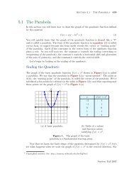
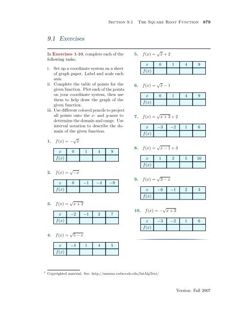
Section 9.1 The Square Root Function 879
9.1 Exercises
In Exercises 1-10, complete each of the
following tasks.
i. Set up a coordinate system on a sheet
of graph paper. Label and scale each
axis.
ii. Complete the table of points for the
given function. Plot each of the points
on your coordinate system, then use
them to help draw the graph of the
given function.
iii. Use different colored pencils to project
all points onto the x- and y-axes to
determine the domain and range. Use
interval notation to describe the domain
of the given function.
1. f(x) = − √ x
x 0 1 4 9
f(x)
2. f(x) = √ −x
x 0 −1 −4 −9
f(x)
3. f(x) = √ x + 2
x −2 −1 2 7
f(x)
5. f(x) = √ x + 2
x 0 1 4 9
f(x)
6. f(x) = √ x − 1
x 0 1 4 9
f(x)
7. f(x) = √ x + 3 + 2
x −3 −2 1 6
f(x)
8. f(x) = √ x − 1 + 3
x 1 2 5 10
f(x)
9. f(x) = √ 3 − x
x −6 −1 2 3
f(x)
10. f(x) = − √ x + 3
x −3 −2 1 6
f(x)
4. f(x) = √ 5 − x
x −4 1 4 5
f(x)
1
Copyrighted material. See: http://msenux.redwoods.edu/IntAlgText/
Version: Fall 2007

880 Chapter 9 Radical Functions
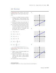
In Exercises 11-20, perform each of the
following tasks.
i. Set up a coordinate system on a sheet
of graph paper. Label and scale each
axis. Remember to draw all lines with
a ruler.
ii. Use geometric transformations to draw
the graph of the given function on
your coordinate system without the
use of a graphing calculator. Note:
You may check your solution with
your calculator, but you should be
able to produce the graph without
the use of your calculator.
iii. Use different colored pencils to project
the points on the graph of the function
onto the x- and y-axes. Use interval
notation to describe the domain
and range of the function.
11. f(x) = √ x + 3
12. f(x) = √ x + 3
13. f(x) = √ x − 2
14. f(x) = √ x − 2
15. f(x) = √ x + 5 + 1
16. f(x) = √ x − 2 − 1
17. f(x) = − √ x + 4
18. f(x) = − √ x + 4
19. f(x) = − √ x + 3
20. f(x) = − √ x + 3
21. To draw the graph of the function
f(x) = √ 3 − x, perform each of the following
steps in sequence without the aid
of a calculator.
i. Set up a coordinate system and sketch
the graph of y = √ x. Label the graph
with its equation.
ii. Set up a second coordinate system
and sketch the graph of y = √ −x.
Label the graph with its equation.
iii. Set up a third coordinate system and
sketch the graph of y = √ −(x − 3).
Label the graph with its equation. This
is the graph of f(x) = √ 3 − x. Use
interval notation to state the domain
and range of this function.
22. To draw the graph of the function
f(x) = √ −x − 3, perform each of the
following steps in sequence.
i. Set up a coordinate system and sketch
the graph of y = √ x. Label the graph
with its equation.
ii. Set up a second coordinate system
and sketch the graph of y = √ −x.
Label the graph with its equation.
iii. Set up a third coordinate system and
sketch the graph of y = √ −(x + 3).
Label the graph with its equation. This
is the graph of f(x) = √ −x − 3. Use
interval notation to state the domain
and range of this function.
23. To draw the graph of the function
f(x) = √ −x − 1, perform each of the
following steps in sequence without the
aid of a calculator.
i. Set up a coordinate system and sketch
the graph of y = √ x. Label the graph
with its equation.
ii. Set up a second coordinate system
and sketch the graph of y = √ −x.
Label the graph with its equation.
iii. Set up a third coordinate system and
sketch the graph of y = √ −(x + 1).
Label the graph with its equation. This
is the graph of f(x) = √ −x − 1. Use
interval notation to state the domain
and range of this function.
Version: Fall 2007

Section 9.1 The Square Root Function 881
24. To draw the graph of the function
f(x) = √ 1 − x, perform each of the following
steps in sequence.
i. Set up a coordinate system and sketch
the graph of y = √ x. Label the graph
with its equation.
ii. Set up a second coordinate system
and sketch the graph of y = √ −x.
Label the graph with its equation.
iii. Set up a third coordinate system and
sketch the graph of y = √ −(x − 1).
Label the graph with its equation. This
is the graph of f(x) = √ 1 − x. Use
interval notation to state the domain
and range of this function.
In Exercises 25-28, perform each of the
following tasks.
i. Draw the graph of the given function
with your graphing calculator.
Copy the image in your viewing window
onto your homework paper. Label
and scale each axis with xmin,
xmax, ymin, and ymax. Label your
graph with its equation. Use the graph
to determine the domain of the function
and describe the domain with interval
notation.
ii. Use a purely algebraic approach to
determine the domain of the given
function. Use interval notation to describe
your result. Does it agree with
the graphical result from part (i)?
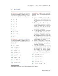
In Exercises 29-40, find the domain of
the given function algebraically.
29. f(x) = √ 2x + 9
30. f(x) = √ −3x + 3
31. f(x) = √ −8x − 3
32. f(x) = √ −3x + 6
33. f(x) = √ −6x − 8
34. f(x) = √ 8x − 6
35. f(x) = √ −7x + 2
36. f(x) = √ 8x − 3
37. f(x) = √ 6x + 3
38. f(x) = √ x − 5
39. f(x) = √ −7x − 8
40. f(x) = √ 7x + 8
25. f(x) = √ 2x + 7
26. f(x) = √ 7 − 2x
27. f(x) = √ 12 − 4x
28. f(x) = √ 12 + 2x
Version: Fall 2007

882 Chapter 9 Radical Functions
9.1 Answers
1. Domain = [0, ∞), Range = (−∞, 0].
x 0 1 4 9
f(x) 0 −1 −2 −3
y
10
5. Domain = [0, ∞), Range = [2, ∞).
x 0 1 4 9
f(x) 2 3 4 5
y
10
f(x)= √ x+2
x
10
x
10
f(x)=− √ x
3. Domain = [−2, ∞), Range = [0, ∞).
x −2 −1 2 7
f(x) 0 1 2 3
y
10
f(x)= √ x+2
7. Domain = [−3, ∞), Range = [2, ∞).
x −3 −2 1 6
f(x) 2 3 4 5
y
10
f(x)= √ x+3+2
x
10
x
10
Version: Fall 2007

Section 9.1 The Square Root Function 883
9. Domain = (−∞, 3], Range = [0, ∞).
15. Domain = [−5, ∞), Range = [1, ∞).
x −6 −1 2 3
f(x) 3 2 1 0
f(x)= √ 3−x
y
10
y
10
f(x)= √ x+5+1
x
10
x
10
17. Domain = [−4, ∞), Range = (−∞, 0].
y
10
11. Domain = [0, ∞), Range = [3, ∞).
y
10
f(x)= √ x+3
x
10
x
10
f(x)=− √ x+4
19. Domain = [0, ∞), Range = (−∞, 3].
y
10
13. Domain = [2, ∞), Range = [0, ∞).
y
10
f(x)= √ x−2
f(x)=− √ x+3
x
10
x
10
Version: Fall 2007

884 Chapter 9 Radical Functions
21. Domain = (−∞, 3], Range = [0, ∞).
27. Domain = (−∞, 3]
y
10
f(x)= √ 12−4x
y
10
f(x)= √ 3−x
x
10
x
−10 3 10
−10
23. Domain = (−∞, −1], Range = [0, ∞).
f(x)= √ −x−1
y
10
x
10
29.
31.
33.
35.
37.
39.
[
−
9
2 , ∞)
( ]
−∞, −
3
8
( ]
−∞, −
4
3
( ]
−∞,
2
7
[
−
1
2 , ∞)
( ]
−∞, −
8
7
25. Domain = [−7/2, ∞)
y
10
f(x)= √ 2x+7
x
−10 −3.5
10
−10
Version: Fall 2007

Section 9.2 Multiplication Properties of Radicals 901
9.2 Exercises
1. Use a calculator to first approximate
√
5
√
2. On the same screen, approximate
√
10. Report the results on your homework
paper.
√2. √Use a calculator to first approximate
7 10. On the same screen, approximate
√ 70. Report the results on your
homework paper.
14.
15.
16.
17.
18.
√
150
√
98
√
252
√
45
√
294
√3. √Use a calculator to first approximate
3 11. On the same screen, approximate
√ 33. Report the results on your
homework paper.
√4. √Use a calculator to first approximate
5 13. On the same screen, approximate
√ 65. Report the results on your
homework paper.
In Exercises 5-20, place each of the radical
expressions in simple radical form.
As in Example 3 in the narrative, check
your result with your calculator.
19.
20.
√
24
√
32
In Exercises 21-26, use prime factorization
(as in Examples 10 and 11 in the
narrative) to assist you in placing the
given radical expression in simple radical
form. Check your result with your
calculator.
21.
22.
√
2016
√
2700
5.
√
18
23.
√
14175
6.
√
80
24.
√
44000
7.
√
112
25.
√
20250
8.
√
72
26.
√
3564
9.
10.
11.
12.
√
108
√
54
√
50
√
48
In Exercises 27-46, place each of the
given radical expressions in simple radical
form. Make no assumptions about
the sign of the variables. Variables can
either represent positive or negative numbers.
13.
√
245
27.
√
(6x − 11) 4
1
Copyrighted material. See: http://msenux.redwoods.edu/IntAlgText/
Version: Fall 2007

902 Chapter 9 Radical Functions
28.
29.
30.
31.
32.
33.
34.
35.
36.
37.
38.
39.
40.
√
16h 8
√
25f 2
√
25j 8
√
16m 2
√
25a 2
√
(7x + 5) 12
√
9w 10
√
25x 2 − 50x + 25
√
49x 2 − 42x + 9
√
25x 2 + 90x + 81
√
25f 14
√
(3x + 6) 12
√
(9x − 8) 12
for x = −2.
49. Given that x < 0, place the radical
expression √ 27x 12 in simple radical
form. Check your solution on your calculator
for x = −2.
50. Given that x < 0, place the radical
expression √ 44x 10 in simple radical
form. Check your solution on your calculator
for x = −2.
In Exercises 51-54, follow the lead of
Example 17 in the narrative to simplify
the given radical expression and check
your result with your graphing calculator.
51. Given that x < 4, place the radical
expression √ x 2 − 8x + 16 in simple
radical form. Use a graphing calculator
to show that the graphs of the original
expression and your simple radical form
agree for all values of x such that x < 4.
41.
42.
43.
44.
45.
46.
√
36x 2 + 36x + 9
√
4e 2
√
4p 10
√
25x 12
√
25q 6
√
16h 12
47. Given that x < 0, place the radical
expression √ 32x 6 in simple radical form.
Check your solution on your calculator
for x = −2.
48. Given that x < 0, place the radical
expression √ 54x 8 in simple radical form.
Check your solution on your calculator
52. Given that x ≥ −2, place the radical
expression √ x 2 + 4x + 4 in simple
radical form. Use a graphing calculator
to show that the graphs of the original
expression and your simple radical form
agree for all values of x such that x ≥ −2.
53. Given that x ≥ 5, place the radical
expression √ x 2 − 10x + 25 in simple
radical form. Use a graphing calculator
to show that the graphs of the original
expression and your simple radical form
agree for all values of x such that x ≥ 5.
54. Given that x < −1, place the radical
expression √ x 2 + 2x + 1 in simple
radical form. Use a graphing calculator
to show that the graphs of the original
expression and your simple radical form
agree for all values of x such that x < −1.
Version: Fall 2007

Section 9.2 Multiplication Properties of Radicals 903
In Exercises 55-72, place each radical
expression in simple radical form. Assume
that all variables represent positive
numbers.
In Exercises 73-80, place each given radical
expression in simple radical form. Assume
that all variables represent positive
numbers.
55.
√
9d 13
73.
√
2f 5 √ 8f 3
56.
√
4k 2
74.
√
3s 3 √ 243s 3
57.
√
25x 2 + 40x + 16
75.
√
2k 7 √ 32k 3
58.
√
9x 2 − 30x + 25
76.
√
2n 9 √ 8n 3
59.
√
4j 11
77.
√
2e 9 √ 8e 3
60.
√
16j 6
78.
√
5n 9 √ 125n 3
61.
√
25m 2
79.
√
3z 5 √ 27z 3
62.
√
9e 9
80.
√
3t 7 √ 27t 3
63.
√
4c 5
64.
√
25z 2
65.
√
25h 10
66.
√
25b 2
67.
√
9s 7
68.
√
9e 7
69.
√
4p 8
70.
√
9d 15
71.
√
9q 10
72.
√
4w 7
Version: Fall 2007

904 Chapter 9 Radical Functions
9.2 Answers
1.
31. 4|m|
33. (7x + 5) 6
35. |5x − 5|
37. |5x + 9|
3.
39. (3x + 6) 6
41. |6x + 3|
43. 2p 4 |p|
45. 5q 2 |q|
47. −4x 3√ 2
5. 3 √ 2
7. 4 √ 7
9. 6 √ 3
11. 5 √ 2
13. 7 √ 5
49. 3x 6√ 3
15. 7 √ 2
17. 3 √ 5
19. 2 √ 6
21. 12 √ 14
23. 45 √ 7
25. 45 √ 10
27. (6x − 11) 2
29. 5|f|
Version: Fall 2007

Section 9.2 Multiplication Properties of Radicals 905
51. −x + 4. The graphs of y = −x +
4 and y = √ x 2 − 8x + 16 follow. Note
that they agree for x < 4.
69. 2p 4
71. 3q 5
73. 4f 4
75. 8k 5
77. 4e 6
79. 9z 4
53. x − 5. The graphs of y = x − 5 and
y = √ x 2 − 10x + 25 follow. Note that
they agree for x ≥ 5.
55. 3d 6√ d
57. 5x + 4
59. 2j 5√ j
61. 5m
63. 2c 2√ c
65. 5h 5
67. 3s 3√ s
Version: Fall 2007

Section 9.3 Division Properties of Radicals 921
9.3 Exercises
√1. √Use a calculator to first approximate
5/ 2. On the same screen, approximate
√ 5/2. Report the results on your
homework paper.
√2. √Use a calculator to first approximate
7/ 5. On the same screen, approximate
√ 7/5. Report the results on your
homework paper.
√3. Use √ a calculator to first approximate
12/ 2. On the same screen, approximate
√ 6. Report the results on your
homework paper.
√4. Use √ a calculator to first approximate
15/ 5. On the same screen, approximate
√ 3. Report the results on your
homework paper.
In Exercises 5-16, place each radical expression
in simple radical form. As in
Example 2 in the narrative, check your
result with your calculator.
√
3
5.
8
6.
7.
8.
9.
10.
√
5
12
√
11
20
√
3
2
√
11
18
√
7
5
11.
12.
13.
14.
15.
16.
√
4
3
√
16
5
√
49
12
√
81
20
√
100
7
√
36
5
In Exercises 17-28, place each radical
expression in simple radical form. As in
Example 4 in the narrative, check your
result with your calculator.
17.
18.
19.
20.
21.
22.
1
√
12
1
√
8
1
√
20
1
√
27
6
√
8
4
√
12
1
Copyrighted material. See: http://msenux.redwoods.edu/IntAlgText/
Version: Fall 2007

922 Chapter 9 Radical Functions
23.
24.
25.
26.
27.
28.
5
√
20
9
√
27
6
2 √ 3
10
3 √ 5
15
2 √ 20
3
2 √ 18
In Exercises 29-36, place the given radical
expression in simple form. Use prime
factorization as in Example 8 in the narrative
to help you with the calculations.
As in Example 6, check your result with
your calculator.
29.
30.
31.
1
√
96
1
√
432
1
√
250
In Exercises 37-44, place each of the
given radical expressions in simple radical
form. Make no assumptions about
the sign of any variable. Variables can
represent either positive or negative numbers.
√
8
37.
x 4
38.
39.
40.
41.
42.
43.
44.
√
12
x 6
√
20
x 2
√
32
x 14
2
√
8x 8
3
√
12x 6
10
√
20x 10
12
√
6x 4
32.
33.
34.
35.
36.
1
√
108
√
5
96
√
2
135
√
2
1485
√
3
280
In Exercises 45-48, follow the lead of
Example 8 in the narrative to craft a solution.
45. Given that x < 0, place the radical
expression 6/ √ 2x 6 in simple radical
form. Check your solution on your calculator
for x = −1.
46. Given that x > 0, place the radical
expression 4/ √ 12x 3 in simple radical
form. Check your solution on your calculator
for x = 1.
Version: Fall 2007

Section 9.3 Division Properties of Radicals 923
47. Given that x > 0, place the radical
expression 8/ √ 8x 5 in simple radical
form. Check your solution on your calculator
for x = 1.
48. Given that x < 0, place the radical
expression 15/ √ 20x 6 in simple radical
form. Check your solution on your
calculator for x = −1.
In Exercises 49-56, place each of the
radical expressions in simple form. Assume
that all variables represent positive
numbers.
49.
√
12
x
50.
√
18
x
51.
52.
53.
54.
55.
56.
√
50
x 3
√
72
x 5
1
√
50x
2
√
18x
3
√
27x 3
5
√
10x 5
Version: Fall 2007

924 Chapter 9 Radical Functions
9.3 Answers
31.
1.
√
10/50
29.
√
6/24
33.
√
30/24
35.
√
330/495
37. 2 √ 2/x 2
3.
39. 2 √ 5/|x|
41.
√
2/(2x 4 )
43.
√
5/(x 4 |x|)
45. −3 √ 2/x 3
47. 2 √ 2x/x 3
5.
√
6/4
49. 2 √ 3x/x
7.
√
55/10
51. 5 √ 2x/x 2
9.
√
22/6
53.
√
2x/(10x)
11. 2 √ 3/3
55.
√
3x/(3x 2 )
13. 7 √ 3/6
15. 10 √ 7/7
17.
√
3/6
19.
√
5/10
21. 3 √ 2/2
23.
√
5/2
25.
√
3
27. 3 √ 5/4
Version: Fall 2007

Section 9.4 Radical Expressions 941
9.4 Exercises
In Exercises 1-14, place each of the radical
expressions in simple radical form.
Check your answer with your calculator.
18. −3(4 − 3 √ 2)
19.
√
2(2 +
√
2)
1. 2(5 √ 7)
2. −3(2 √ 3)
3. − √ 3(2 √ 5)
20.
21.
22.
√
3(4 −
√
6)
√
2(
√
10 +
√
14)
√
3(
√
15 −
√
33)
4.
5.
6.
√
2(3
√
7)
√
3(5
√
6)
√
2(−3
√
10)
In Exercises 23-30, combine like terms.
Place your final answer in simple radical
form. Check your solution with your calculator.
7. (2 √ 5)(−3 √ 3)
8. (−5 √ 2)(−2 √ 7)
9. (−4 √ 3)(2 √ 6)
23. −5 √ 2 + 7 √ 2
24. 2 √ 3 + 3 √ 3
25. 2 √ 6 − 8 √ 6
10. (2 √ 5)(−3 √ 10)
26.
√
7 − 3
√
7
11. (2 √ 3) 2
12. (−3 √ 5) 2
13. (−5 √ 2) 2
14. (7 √ 11) 2
In Exercises 15-22, use the distributive
property to multiply. Place your final
answer in simple radical form. Check
your result with your calculator.
27. 2 √ 3 − 4 √ 2 + 3 √ 3
28. 7 √ 5 + 2 √ 7 − 3 √ 5
29. 2 √ 3 + 5 √ 2 − 7 √ 3 + 2 √ 2
30. 3 √ 11 − 2 √ 7 − 2 √ 11 + 4 √ 7
In Exercises 31-40, combine like terms
where possible. Place your final answer
in simple radical form. Use your calculator
to check your result.
15. 2(3 + √ 5)
31.
√
45 +
√
20
16. −3(4 − √ 7)
17. 2(−5 + 4 √ 2)
32. −4 √ 45 − 4 √ 20
33. 2 √ 18 − √ 8
1
Copyrighted material. See: http://msenux.redwoods.edu/IntAlgText/
Version: Fall 2007

942 Chapter 9 Radical Functions
34. − √ 20 + 4 √ 45
35. −5 √ 27 + 5 √ 12
36. 3 √ 12 − 2 √ 27
37. 4 √ 20 + 4 √ 45
38. −2 √ 18 − 5 √ 8
39. 2 √ 45 + 5 √ 20
40. 3 √ 27 − 4 √ 12
In Exercises 41-48, simplify each of the
given rational expressions. Place your final
answer in simple radical form. Check
your result with your calculator.
41.
√
2 −
1 √2
42. 3 √ 3 − 3 √
3
43. 2 √ 2 − 2 √
2
44. 4 √ 5 − 5 √
5
45. 5 √ 2 + 3 √
2
46. 6 √ 3 + 2 √
3
47.
48.
√
8 −
12
√
2
− 3 √ 2
√
27 −
6 √3 − 5 √ 3
In Exercises 49-60, multiply to expand
each of the given radical expressions. Place
your final answer in simple radical form.
Use your calculator to check your result.
49. (2 + √ 3)(3 − √ 3)
50. (5 + √ 2)(2 − √ 2)
51. (4 + 3 √ 2)(2 − 5 √ 2)
52. (3 + 5 √ 3)(1 − 2 √ 3)
53. (2 + 3 √ 2)(2 − 3 √ 2)
54. (3 + 2 √ 5)(3 − 2 √ 5)
55. (2 √ 3 + 3 √ 2)(2 √ 3 − 3 √ 2)
56. (8 √ 2 + √ 5)(8 √ 2 − √ 5)
57. (2 + √ 5) 2
58. (3 − √ 2) 2
59. ( √ 3 − 2 √ 5) 2
60. (2 √ 3 + 3 √ 2) 2
In Exercises 61-68, place each of the
given rational expressions in simple radical
form by “rationalizing the denominator.”
Check your result with your calculator.
61.
62.
63.
1
√
5 +
√
3
1
2 √ 3 − √ 2
6
2 √ 5 − √ 2
64.
9
3 √ 3 − √ 6
Version: Fall 2007

Section 9.4 Radical Expressions 943
65.
66.
67.
68.
2 + √ 3
2 − √ 3
3 − √ 5
3 + √ 5
√ √
3 + 2
√ √
3 − 2
2 √ 3 + √ 2
√
3 −
√
2
In Exercises 69-76, use the quadratic
formula to find the solutions of the given
equation. Place your solutions in simple
radical form and reduce your solutions to
lowest terms.
69. 3x 2 − 8x = 5
70. 5x 2 − 2x = 1
78. Given f(x) = √ x + 2, evaluate the
expression
f(x) − f(3)
,
x − 3
and then “rationalize the numerator.”
79. Given f(x) = √ x, evaluate the expression
f(x + h) − f(x)
,
h
and then “rationalize the numerator.”
80. Given f(x) = √ x − 3, evaluate the
expression
f(x + h) − f(x)
,
h
and then “rationalize the numerator.”
71. 5x 2 = 2x + 1
72. 3x 2 − 2x = 11
73. 7x 2 = 6x + 2
74. 11x 2 + 6x = 4
75. x 2 = 2x + 19
76. 100x 2 = 40x − 1
In Exercises 77-80, we will suspend the
usual rule that you should rationalize the
denominator. Instead, just this one time,
rationalize the numerator of the resulting
expression.
77. Given f(x) = √ x, evaluate the expression
f(x) − f(2)
,
x − 2
and then “rationalize the numerator.”
Version: Fall 2007

944 Chapter 9 Radical Functions
9.4 Answers
1. 10 √ 7
45. 13 √ 2/2
43.
√
2
3. −2 √ 15
47. −7 √ 2
5. 15 √ 2
49. 3 + √ 3
7. −6 √ 15
51. −22 − 14 √ 2
9. −24 √ 2
53. −14
11. 12
55. −6
13. 50
57. 9 + 4 √ 5
15. 6 + 2 √ 5
59. 23 − 4 √ 15
17. −10 + 8 √ √ √
2
5 − 3
19. 2 √ 61.
2
2 + 2
21. 2 √ 5 + 2 √ 2 √ 5 + √ 2
63.
7
3
23. 2 √ 2
65. 7 + 4 √ 3
25. −6 √ 6
67. 5 + 2 √ 6
27. 5 √ 3 − 4 √ 2
69. (4 ± √ 31)/3
29. 7 √ 2 − 5 √ 3
71. (1 ± √ 6)/5
31. 5 √ 5
73. (3 ± √ 23)/7
33. 4 √ 2
75. 1 ± 2 √ 5
35. −5 √ 3
1
77. √ √
37. 20 √ x + 2
5
39. 16 √ 1
79. √ √
5
x + h + x
41.
√
2/2
Version: Fall 2007

Section 9.5 Radical Equations 955
9.5 Exercises
For the rational functions in Exercises 1-
6, perform each of the following tasks.
i. Load the function f and the line y =
k into your graphing calculator. Adjust
the viewing window so that all
point(s) of intersection of the two graphs
are visible in your viewing window.
ii. Copy the image in your viewing window
onto your homework paper. Label
and scale each axis with xmin,
xmax, ymin, and ymax. Label the
graphs with their equations. Remember
to draw all lines with a ruler.
iii. Use the intersect utility to determine
the coordinates of the point(s)
of intersection. Plot the point of intersection
on your homework paper
and label it with its coordinates.
iv. Solve the equation f(x) = k algebraically.
Place your work and solution
next to your graph. Do the
solutions agree?
1. f(x) = √ x + 3, k = 2
2. f(x) = √ 4 − x, k = 3
3. f(x) = √ 7 − 2x, k = 4
4. f(x) = √ 3x + 5, k = 5
5. f(x) = √ 5 + x, k = 4
6. f(x) = √ 4 − x, k = 5
In Exercises 7-12, use an algebraic technique
to solve the given equation. Check
your solutions.
8.
9.
10.
11.
12.
√
4x + 6 = 7
√ 6x − 8 = 8
√
2x + 4 = 2
√ −3x + 1 = 3
√
4x + 7 = 3
For the rational functions in Exercises 13-
16, perform each of the following tasks.
i. Load the function f and the line y =
k into your graphing calculator. Adjust
the viewing window so that all
point(s) of intersection of the two graphs
are visible in your viewing window.
ii. Copy the image in your viewing window
onto your homework paper. Label
and scale each axis with xmin,
xmax, ymin, and ymax. Label the
graphs with their equations. Remember
to draw all lines with a ruler.
iii. Use the intersect utility to determine
the coordinates of the point(s)
of intersection. Plot the point of intersection
on your homework paper
and label it with its coordinates.
iv. Solve the equation f(x) = k algebraically.
Place your work and solution
next to your graph. Do the
solutions agree?
13. f(x) = √ x + 3 + x, k = 9
14. f(x) = √ x + 6 − x, k = 4
15. f(x) = √ x − 5 − x, k = −7
7.
√ −5x + 5 = 2
16. f(x) = √ x + 5 + x, k = 7
1
Copyrighted material. See: http://msenux.redwoods.edu/IntAlgText/
Version: Fall 2007

956 Chapter 9 Radical Functions
In Exercises 17-24, use an algebraic technique
to solve the given equation. Check
your solutions.
17.
18.
19.
20.
21.
22.
23.
24.
√ x + 1 + x = 5
√ x + 8 − x = 8
√
x + 4 + x = 8
√ x + 8 − x = 2
√ x + 5 − x = 3
√ x + 5 + x = 7
√ x + 9 − x = 9
√
x + 7 + x = 5
For the rational functions in Exercises 25-
28, perform each of the following tasks.
i. Load the function f and the line y =
k into your graphing calculator. Adjust
the viewing window so that all
point(s) of intersection of the two graphs
are visible in your viewing window.
ii. Copy the image in your viewing window
onto your homework paper. Label
and scale each axis with xmin,
xmax, ymin, and ymax. Label the
graphs with their equations. Remember
to draw all lines with a ruler.
iii. Use the intersect utility to determine
the coordinates of the point(s)
of intersection. Plot the point of intersection
on your homework paper
and label it with its coordinates.
iv. Solve the equation f(x) = k algebraically.
Place your work and solution
next to your graph. Do the
solutions agree?
27. f(x) = √ x + 2 + √ 3x + 4, k = 2
28. f(x) = √ 6x + 7 + √ 3x + 3, k = 1
In Exercises 29-40, use an algebraic technique
to solve the given equation. Check
your solutions.
29.
30.
31.
32.
33.
34.
35.
36.
37.
38.
39.
40.
√
x + 46 −
√ x − 35 = 1
√ x − 16 +
√ x + 16 = 8
√ x − 19 +
√ x − 6 = 13
√ x + 31 −
√ x + 12 = 1
√ x − 2 −
√
x − 49 = 1
√ x + 13 +
√ x + 8 = 5
√
x + 27 −
√ x − 22 = 1
√ x + 10 +
√ x + 13 = 3
√ x + 30 −
√ x − 38 = 2
√ x + 36 −
√ x + 11 = 1
√
x − 17 +
√ x + 3 = 10
√ x + 18 +
√ x + 13 = 5
25. f(x) = √ x − 1 + √ x + 6, k = 7
26. f(x) = √ x + 2 + √ x + 9, k = 7
Version: Fall 2007

Section 9.5 Radical Equations 957
9.5 Answers
1. x = 1
y
10
7.
1
5
9. 12
(1,2)
f(x)= √ x+3
y=2
x
10
11. − 8 3
13. x = 6
20
y
f(x)= √ x+3+x
(6,9)
y=9
3. x = −9/2
y
10
x
20
f(x)= √ 7−2x
(−4.5,4)
y=4
x
10
15. x = 9
20
y
5. x = 11
10
y
x
20
(11,4)
f(x)= √ x+5
y=4
(9,−7)
y=−7
x
20
f(x)= √ x−5−x
17. 3
19. 5
21. −1
Version: Fall 2007

958 Chapter 9 Radical Functions
23. −8, −9
25. x = 10
20
y
f(x)= √ x−1+ √ x+6
(10,7)
y=7
x
20
27. x = −1
20
y
f(x)= √ x+2+ √ 3x+4
(−1,2)
y=2
x
20
29. 1635
31. 55
33. 578
35. 598
37. 294
39. 33
Version: Fall 2007

Section 9.6 The Pythagorean Theorem 971
9.6 Exercises
In Exercises 1-8, state whether or not
the given triple is a Pythagorean Triple.
Give a reason for your answer.
10.
1. (8, 15, 17)
2
2. (7, 24, 25)
3. (8, 9, 17)
2
4. (4, 9, 13)
11.
5. (12, 35, 37)
6. (12, 17, 29)
7. (11, 17, 28)
4
8
8. (11, 60, 61)
In Exercises 9-16, set up an equation
to model the problem constraints and solve.
Use your answer to find the missing side
of the given right triangle. Include a
sketch with your solution and check your
result.
9.
12.
13.
10
12
2 √ 3
2
2 √ 3
2
1
Copyrighted material. See: http://msenux.redwoods.edu/IntAlgText/
Version: Fall 2007

972 Chapter 9 Radical Functions
14.
legs.
12
4 √ 3
20. One leg of a right triangle is 3 feet
longer than 3 times the length of the first
leg. The length of the hypotenuse is 25
feet. Find the lengths of the legs.
15.
21. Pythagoras is credited with the following
formulae that can be used to generate
Pythagorean Triples.
16.
5
10
a = m
b = m2 − 1
,
2
c = m2 + 1
2
8
8 √ 2
Use the technique of Example 6 to demonstrate
that the formulae given above will
generate Pythagorean Triples, provided
that m is an odd positive integer larger
than one. Secondly, generate at least
3 instances of Pythagorean Triples with
Pythagoras’s formula.
In Exercises 17-20, set up an equation
that models the problem constraints. Solve
the equation and use the result to answer
the question. Look back and check your
result.
17. The legs of a right triangle are consecutive
positive integers. The hypotenuse
has length 5. What are the lengths of the
legs?
18. The legs of a right triangle are consecutive
even integers. The hypotenuse
has length 10. What are the lengths of
the legs?
22. Plato (380 BC) is credited with the
following formulae that can be used to
generate Pythagorean Triples.
a = 2m
b = m 2 − 1,
c = m 2 + 1
Use the technique of Example 6 to demonstrate
that the formulae given above will
generate Pythagorean Triples, provided
that m is a positive integer larger than
1. Secondly, generate at least 3 instances
of Pythagorean Triples with Plato’s formula.
19. One leg of a right triangle is 1 centimeter
less than twice the length of the
first leg. If the length of the hypotenuse
is 17 centimeters, find the lengths of the
Version: Fall 2007

Section 9.6 The Pythagorean Theorem 973
In Exercises 23-28, set up an equation
that models the problem constraints. Solve
the equation and use the result to answer
the question. Look back and check your
result.
23. Fritz and Greta are planting a 12-
foot by 18-foot rectangular garden, and
are laying it out using string. They would
like to know the length of a diagonal to
make sure that right angles are formed.
Find the length of a diagonal. Approximate
your answer to within 0.1 feet.
24. Angelina and Markos are planting
a 20-foot by 28-foot rectangular garden,
and are laying it out using string. They
would like to know the length of a diagonal
to make sure that right angles are
formed. Find the length of a diagonal.
Approximate your answer to within 0.1
feet.
25. The base of a 36-foot long guy wire
is located 16 feet from the base of the
telephone pole that it is anchoring. How
high up the pole does the guy wire reach?
Approximate your answer to within 0.1
feet.
26. The base of a 35-foot long guy wire
is located 10 feet from the base of the
telephone pole that it is anchoring. How
high up the pole does the guy wire reach?
Approximate your answer to within 0.1
feet.
27. A stereo receiver is in a corner of
a 13-foot by 16-foot rectangular room.
Speaker wire will run under a rug, diagonally,
to a speaker in the far corner. If 3
feet of slack is required on each end, how
long a piece of wire should be purchased?
Approximate your answer to within 0.1
feet.
28. A stereo receiver is in a corner of
a 10-foot by 15-foot rectangular room.
Speaker wire will run under a rug, diagonally,
to a speaker in the far corner. If 4
feet of slack is required on each end, how
long a piece of wire should be purchased?
Approximate your answer to within 0.1
feet.
In Exercises 29-38, use the distance formula
to find the exact distance between
the given points.
29. (−8, −9) and (6, −6)
30. (1, 0) and (−9, −2)
31. (−9, 1) and (−8, 7)
32. (0, 9) and (3, 1)
33. (6, −5) and (−9, −2)
34. (−9, 6) and (1, 4)
35. (−7, 7) and (−3, 6)
36. (−7, −6) and (−2, −4)
37. (4, −3) and (−9, 6)
38. (−7, −1) and (4, −5)
In Exercises 39-42, set up an equation
that models the problem constraints. Solve
the equation and use the result to answer
the question. Look back and check your
result.
39. Find k so that the point (4, k) is
2 √ 2 units away from the point (2, 1).
40. Find k so hat the point (k, 1) is
2 √ 2 units away from the point (0, −1).
Version: Fall 2007

974 Chapter 9 Radical Functions
41. Find k so that the point (k, 1) is
√
17 units away from the point (2, −3).
42. Find k so that the point (−1, k) is
√
13 units away from the point (−4, −3).
43. Set up a coordinate system on a
sheet of graph paper. Label and scale
each axis. Plot the points P (0, 5) and
Q(4, −3) on your coordinate system.
a) Plot several points that are equidistant
from the points P and Q on your
coordinate system. What graph do
you get if you plot all points that are
equidistant from the points P and Q?
Determine the equation of the graph
by examining the resulting image on
your coordinate system.
b) Use the distance formula to find the
equation of the graph of all points
that are equidistant from the points
P and Q. Hint: Let (x, y) represent
an arbitrary point on the graph of all
points equidistant from points P and
Q. Calculate the distances from the
point (x, y) to the points P and Q
separately, then set them equal and
simplify the resulting equation. Note
that this analytical approach should
provide an equation that matches that
found by the graphical approach in
part (a).
44. Set up a coordinate system on a
sheet of graph paper. Label and scale
each axis. Plot the point P (0, 2) and label
it with its coordinates. Draw the line
y = −2 and label it with its equation.
a) Plot several points that are equidistant
from the point P and the line
y = −2 on your coordinate system.
What graph do you get if you plot
all points that are equidistant from
the points P and the line y = −2.
b) Use the distance formula to find the
equation of the graph of all points
that are equidistant from the points
P and the line y = −2. Hint: Let
(x, y) represent an arbitrary point on
the graph of all points equidistant from
points P and the line y = −2. Calculate
the distances from the point
(x, y) to the points P and the line y =
−2 separately, then set them equal
and simplify the resulting equation.
Version: Fall 2007

Section 9.6 The Pythagorean Theorem 975
45. Copy the following figure onto a
sheet of graph paper. Cut the pieces of
the first figure out with a pair of scissors,
then rearrange them to form the
second figure. Explain how this proves
the Pythagorean Theorem.
46. Compare this image to the one that
follows and explain how this proves the
Pythagorean Theorem.
b
a
a
c
c
b
b
c
c
a
a
b
b
a
b
c
b
a
c
a
b
a
Version: Fall 2007

976 Chapter 9 Radical Functions
9.6 Answers
1. Yes, because 8 2 + 15 2 = 17 2
3. No, because 8 2 + 9 2 ≠ 17 2
5. Yes, because 12 2 + 35 2 = 37 2
43.
a) In the figure that follows, XP = XQ.
y
10
7. No, because 11 2 + 17 2 ≠ 28 2
9. 4
11. 4 √ 3
P (0,5)
X(x,y)
y=(1/2)x
13. 2 √ 2
x
−5 10
15. 5 √ 3
17. The legs have lengths 3 and 4.
19. The legs have lengths 8 and 15 centimeters.
21. (3, 4, 5), (5, 12, 13), and (7, 24, 25),
with m = 3, 5, and 7, respectively.
23. 21.63 ft
25. 32.25 ft
27. 26.62 ft
−5
b) y = (1/2)x
Q(4,−3)
29.
31.
33.
35.
37.
√
205
√
37
√ √
234 = 3 26
√
17
√ √
250 = 5 10
39. k = 3, −1.
41. k = 1, 3.
Version: Fall 2007