Important Discrete and Continuous Probability Distributions

BMED2803, BV
Probability Distributions
Discrete Distributions
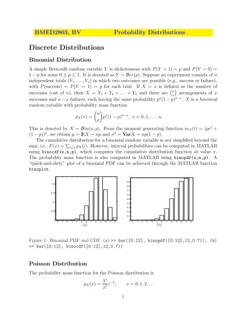
Binomial Distribution
A simple Bernoulli random variable Y is dichotomous with P (Y = 1) = p and P (Y = 0) =
1 − p for some 0 ≤ p ≤ 1. It is denoted as Y ∼ Ber(p). Suppose an experiment consists of n
independent trials (Y 1 , . . . , Y n ) in which two outcomes are possible (e.g., success or failure),
with P (success) = P (Y = 1) = p for each trial. If X = x is defined as the number of
successes (out of n), then X = Y 1 + Y 2 + . . . + Y n and there are ( )
n
x arrangements of x
successes and n − x failures, each having the same probability p x (1 − p) n−x . X is a binomial
random variable with probability mass function
( n
x)
p X (x) =
p x (1 − p) n−x , x = 0, 1, . . . , n.
This is denoted by X ∼ Bin(n, p). From the moment generating function m X (t) = (pe t +
(1 − p)) n , we obtain µ = IEX = np and σ 2 = VarX = np(1 − p).
The cumulative distribution for a binomial random variable is not simplified beyond the
sum; i.e., F (x) = ∑ i≤x p X (i). However, interval probabilities can be computed in MATLAB
using binocdf(x,n,p), which computes the cumulative distribution function at value x.
The probability mass function is also computed in MATLAB using binopdf(x,n,p). A
“quick-and-dirty” plot of a binomial PDF can be achieved through the MATLAB function
binoplot.
1
0.2
0.15
0.1
0.05
0.9
0.8
0.7
0.6
0.5
0.4
0.3
0.2
0.1
0
0 1 2 3 4 5 6 7 8 9 10 11 12
(a)
0
0 1 2 3 4 5 6 7 8 9 10 11 12
(b)
Figure 1: Binomial PDF and CDF. (a) >> bar([0:12], binopdf([0:12],12,0.7)); (b)
>> bar([0:12], binocdf([0:12],12,0.7))
Poisson Distribution
The probability mass function for the Poisson distribution is
p X (x) = λx
x! e−λ , x = 0, 1, 2, . . .
1

This is denoted by X ∼ Poi(λ). From m X (t) = exp{λ(e t − 1)}, we have IEX = λ and
VarX = λ; the mean and the variance coincide.
The sum of a finite independent set of Poisson variables is also Poisson. Specifically, if
X i ∼ Poi(λ i ), then Y = X 1 + . . . + X k is distributed as Poi(λ 1 + . . . + λ k ). Furthermore,
the Poisson distribution is a limiting form for a binomial model, i.e.,
lim
n,np→∞,λ
( n
x
)
p x (1 − p) n−x = 1 x! λx e −λ . (1)
MATLAB commands for Poisson CDF, PDF, quantile, and a random number are: poisscdf,
poisspdf, poissinv, and poissrnd.
0.2
0.9
0.8
0.15
0.1
0.05
0.7
0.6
0.5
0.4
0.3
0.2
0.1
0
0 1 2 3 4 5 6 7 8 9 10 11 12
(a)
0
0 1 2 3 4 5 6 7 8 9 10 11 12
(b)
Figure 2: Poisson PDF and CDF. (a) >> bar([0:12], poisspdf([0:12],3)); (b) >>
bar([0:12], poisscdf([0:12],3))
Negative Binomial Distribution
Suppose we are dealing with i.i.d. trials again, this time counting the number of failures
observed until a fixed number of successes (k) occur. If we observe k consecutive successes at
the start of the experiment, for example, the count is X = 0 and P X (0) = p k , where p is the
probability of success. If X = x, we have observed x failures and k successes in x + k trials.
There are ( )
x+k
x different ways of arranging those x + k trials, but we can only be concerned
with ( the ) arrangements in which the last trial ended in a success. So there are really only
x+k−1
arrangements, each equal in probability. With this in mind, the probability mass
x
function is
( ) k + x − 1
p X (x) =
p k (1 − p) x , x = 0, 1, 2, . . .
x
This is denoted by X ∼ N B(k, p).
From its moment generating function
(
) k
p
m(t) =
,
1 − (1 − p)e t
2

the expectation of a negative binomial random variable is IEX = k(1 − p)/p and variance
VarX = k(1 − p)/p 2 . MATLAB commands for negative binomial CDF, PDF, quantile, and
a random number are: nbincdf, nbinpdf, nbininv, and nbinrnd.
0.2
0.18
0.16
0.14
0.12
0.9
0.8
0.7
0.6
0.1
0.5
0.08
0.4
0.06
0.3
0.04
0.2
0.02
0.1
0
0 1 2 3 4 5 6 7 8 9 10 11 12
(a)
0
0 1 2 3 4 5 6 7 8 9 10 11 12
(b)
Figure 3: Negative Binomial PDF and CDF. (a) >> bar([0:12],
nbinpdf([0:12],4,0.6)); (b) >> bar([0:12], nbincdf([0:12],4,0.6))
Geometric Distribution
The special case of negative binomial for k = 1 is called the geometric distribution, that
is, in repeated independent trials we are interested in the number of failures before the first
success.
Random variable X has geometric Ge(p) distribution if its probability mass function is
p X (x) = p(1 − p) x , x = 0, 1, 2, . . .
If X has geometric Ge(p) distribution, its expected value is IEX = (1 − p)/p and variance
VarX = (1 − p)/p 2 . The geometric random variable can be considered as the discrete
analog to the (continuous) exponential random variable because it possesses a “memoryless”
property. That is, if we condition on X ≥ m for some non-negative integer m, then for
n ≥ m, P (X ≥ n|X ≥ m) = P (X ≥ n − m). MATLAB commands for geometric CDF,
PDF, quantile, and a random number are: geocdf, geopdf, geoinv, and geornd.
Hypergeometric Distribution
Suppose a box contains m balls, k of which are white and m − k of which are gold. Suppose
we randomly select and remove n balls from the box without replacement, so that when we
finish, there are only m − n balls left. If X is the number of white balls chosen (without
replacement) from n, then
)
p X (x) =
( )( k m−k
x n−x
( m
n) , x ∈ {0, 1, . . . , min{n, k}}.
This is denoted by X ∼ HG(m, k, n).
3

0.4
0.35
0.3
0.25
0.2
0.15
0.1
0.05
0
0 1 2 3 4 5 6 7 8 9 10 11 12
(a)
0.9
0.8
0.7
0.6
0.5
0.4
0.3
0.2
0.1
0
0 1 2 3 4 5 6 7 8 9 10 11 12
(b)
Figure 4: Geometric PDF and CDF. (a) >> bar([0:12], geopdf([0:12],0.4)); (b) >>
bar([0:12], geocdf([0:12],0.4))
This probability mass function can be deduced with counting rules. There are ( )
m
n
different ways of selecting the n balls from a box of m. From these (each equally likely),
there are ( )
k
x ways of selecting x white balls from the k white balls in the box, and similarly
( ) m−k
n−x ways of choosing the gold balls.
It can be shown that the mean and variance for the hypergeometric distribution are,
respectively,
µ = nk
( ) ( ) (m )
nk m − k − n
m and σ2 =
.
m m m − 1
MATLAB commands for Hypergeometric CDF, PDF, quantile, and a random number are:
hygecdf, hygepdf, hygeinv, and hygernd.
1
0.25
0.9
0.8
0.2
0.7
0.15
0.6
0.5
0.1
0.4
0.3
0.05
0.2
0.1
0
0 1 2 3 4 5 6 7 8 9 10 11 12
(a)
0
0 1 2 3 4 5 6 7 8 9 10 11 12
(b)
Figure 5: Hypergeometric PDF and CDF. (a) >> bar([0:12],
hygepdf([0:12],30,15,12)); (b) >> bar([0:12], hygecdf([0:12],30,15,12))
Multinomial Distribution
The Binomial distribution was based on dichotomizing event outcomes. If the outcomes can
be classified into k ≥ 2 categories, then out of n trials, we have X i outcomes falling in the
4

category i, i = 1, . . . , k. The probability mass function for the vector (X 1 , . . . , X k ) is
p X1 ,...,X k
(x 1 , ..., x k ) =
n!
x 1 ! · · · x k ! p 1 x1 · · · p k
x k
,
where p 1 + . . . + p k = 1, so there are k − 1 free probability parameters to characterize the
multivariate distribution. This is denoted by X = (X 1 , . . . , X k ) ∼ Mn(n, p 1 , . . . , p k ).
The mean and variance of X i is the same as a binomial since this is the marginal distribution
of X i , i.e., IE(X i ) = np i , Var(X i ) = np i (1 − p i ). The covariance between X i
and X j is Cov(X i , X j ) = −np i p j because IE(X i X j ) = IE(IE(X i X j |X j )) = IE(X j IE(X i |X j ))
and conditional on X j = x j , X i is binomial Bin(n − x j , p i /(1 − p j )). Thus, IE(X i X j ) =
IE(X j (n − X j ))p i /(1 − p j ), and the covariance follows from this.
Continuous Distributions
Exponential Distribution
The probability density function for an exponential random variable is
f X (x) = 1 β e−x/β , x > 0, β > 0.
An exponentially distributed random variable X is denoted by X ∼ E(β). Its moment
generating function is m(t) = 1/(1 − βt) for t < 1/β, and the mean and variance are β and
β 2 , respectively. This distribution has several interesting features - for example, its failure
rate, defined as
r X (x) =
f X(x)
1 − F X (x) ,
is constant and equal to 1/β.
The exponential distribution has an important connection to the Poisson distribution.
Suppose we measure i.i.d. exponential E(β) outcomes (X 1 , X 2 , . . .), and define S n = X 1 +
. . . + X n . For any positive value t, it can be shown that P (S n < t < S n+1 ) = p Y (n), where
p Y (n) is the probability mass function for a Poisson random variable Y with parameter t/β.
Similar to a geometric random variable, an exponential random variable has the memoryless
property because for t > x, P (X ≥ t|X ≥ x) = P (X ≥ t − x).
The median value, representing a typical observation, is roughly 70% of the mean, showing
how extreme values can affect the population mean. This is easily shown because of the ease
at which the inverse CDF is computed:
p ≡ F X (x; β) = 1 − e −x/β
⇐⇒ F X −1 (p) ≡ x p = −β log(1 − p).
MATLAB commands for Exponential CDF, PDF, quantile, and a random number are:
expcdf, exppdf, expinv, and exprnd. For example, the CDF of random variable X with
E(3) distribution evaluated at x = 2 is calculated in MATLAB as expcdf(2, 3).
Often, the exponential random variable is parameterized by a reciprocal of its scale,
λ = 1/β. In that case, the density is given by
f X (x) = λe −λx , x > 0, λ > 0.
5

1
0.5
0.4
0.3
0.2
0.1
0
−1 0 1 2 3 4 5 6
(a)
0.9
0.8
0.7
0.6
0.5
0.4
0.3
0.2
0.1
0
−1 0 1 2 3 4 5 6
(b)
Figure 6: Exponential PDF and CDF. (a) >> x=0:0.01:6; plot(x, exppdf(x,2));
(b)>> plot(x, expcdf(x,2))
Gamma Distribution
The gamma distribution is an extension of the exponential distribution. Random variable
X has gamma Ga(α, β) distribution if its probability density function is given by
f X (x) =
1
β α Γ(α) xα−1 e −x/β , x > 0, α > 0, β > 0.
The moment generating function is m(t) = (1/(1 − βt)) α , so in the case α = 1, gamma is
precisely the exponential distribution. From m(t) we have IEX = αβ and VarX = αβ 2 .
If X 1 , . . . , X n are generated from an exponential distribution with scale parameter β,
it follows from m(t) that Y = X 1 + . . . + X n is distributed gamma with parameters n
and β; that is, Y ∼ Ga(n, β). As we mentioned, exponential E(β) distribution is Ga(1, β),
Erlang distribution (used in queueing theory) is Ga(α, 1) and χ 2 -distribution with k degrees
of freedom is Ga(k/2, 2). The CDF in MATLAB is gamcdf(x, alpha, beta), and the
PDF is gampdf(x, alpha, beta). The function gaminv(p, alpha, beta) computes the
p th quantile of the Ga(α, β).
1
0.9
0.8
0.1
0.7
0.6
0.5
0.05
0.4
0.3
0.2
0.1
0
0 2 4 6 8 10 12 14 16 18
(a)
0
0 2 4 6 8 10 12 14 16 18
(b)
Figure 7: Gamma PDF and CDF. (a) >> x=0:0.01:18; plot(x, gampdf(x,2,3)); (b)>>
plot(x, gamcdf(x,2,3))
6

As in the Exponential distribution there is an alternative parametrization for Gamma
distribution that is often used. In this case the scale parameter β is replaced by a “rate”
parameter λ = 1/β, and the corresponding density is given as
f X (x) =
λα
Γ(α) xα−1 e −λx , x > 0, α > 0, λ > 0.
In this parametrization, IEX = α/λ and VarX = α/λ 2 .
Normal Distribution
The probability density function for a normal random variable with mean µ and variance σ 2
is
f X (x) =
1
√
2πσ
2 e− 1
2σ 2 (x−µ)2 , ∞ < x < ∞.
The distribution function is computed using integral approximation because no closed form
exists for the anti-derivative; this is generally not a problem for practitioners because most
software packages will compute interval probabilities numerically. For example, in MATLAB,
normcdf(x, mu, sigma) and normpdf(x, mu, sigma) find the CDF and PDF at x, and
norminv(p, mu, sigma) computes the inverse CDF with quantile probability p. A random
variable X with the normal distribution will be denoted X ∼ N (µ, σ 2 ).
The Central Limit Theorem elevates the status of the normal distribution above other
distributions. Despite its difficult formulation, the normal is one of the most important
distributions in all science, and it has a critical role to play in nonparametric statistics.
Any linear combination of normal random variables (independent or with simple covariance
structures) are also normally distributed. In such sums, then, we need only keep track of
the mean and variance, since these two parameters completely characterize the distribution.
For example, if X 1 , . . . , X n are i.i.d. N (µ, σ 2 ), then the sample mean ¯X = (X 1 + . . . + X n )/n
has normal N (µ, σ 2 /n) distribution.
Chi-square Distribution
The probability density function for an chi-square random variable with the parameter k,
called the degrees of freedom, is is
f X (x) = 2−k/2
Γ(k/2) xk/2−1 e −x/2 , − ∞ < x < ∞.
The chi-square distribution (χ 2 ) is a special case of the Gamma distribution with parameters
α = k/2 and β = 2. Its mean and variance are µ = k and σ 2 = 2k.
If Z ∼ N (0, 1), then Z 2 ∼ χ 2 1, that is, a chi-square random variable with one degree-offreedom.
Furthermore, if U ∼ χ 2 m and V ∼ χ 2 n are independent, then U + V ∼ χ 2 m+n.
From these results, it can be shown that if X 1 , . . . , X n ∼ N (µ, σ 2 ) and ¯X is the sample
mean, then the sample variance S 2 = ∑ i(X i − ¯X) 2 /(n − 1) is proportional to a chi-square
7

andom variable with n − 1 degrees of freedom:
(n − 1)S 2
σ 2
∼ χ 2 n−1.
In MATLAB, the CDF and PDF for a χ 2 k is chi2cdf(x,k) and chi2pdf(x,k). The p th
quantile of the χ 2 k distribution is chi2inv(p,k).
(Student) t - Distribution
Random variable X has Student’s t distribution with k degrees of freedom, X ∼ t k , if its
probability density function is
f X (x) = Γ ( )
k+1 ( ) −
k+1
2
√ 1 + x2 2
, −∞ < x < ∞.
kπ Γ(k/2) k
The t-distribution 1 is similar in shape to the standard normal distribution except for the
fatter tails. If X ∼ t k , IEX = 0, k > 1 and VarX = k/(k − 2), k > 2. For k = 1, Student t
distribution coincides with Cauchy distribution.
The t-distribution has an important role to play in statistical inference. With a set of i.i.d.
X 1 , . . . , X n ∼ N (µ, σ 2 ), we can standardize the sample mean using the simple transformation
of Z = ( ¯X − µ)/σ ¯X = √ n( ¯X − µ)/σ. However, if the variance is unknown, by using the
same transformation except substituting the sample standard deviation S for σ, we arrive
at a t-distribution with n − 1 degrees of freedom:
T = ( ¯X − µ)
S/ √ n ∼ t n−1
√
More technically, if Z ∼ N (0, 1) and Y ∼ χ 2 k are independent, then T = Z/ Y/k ∼ t k .
In MATLAB, the CDF at x for a t-distribution with k degrees of freedom is calculated as
tcdf(x,k), and the PDF is computed as tpdf(x,k). The p th percentile is computed with
tinv(p,k).
F Distribution
Random variable X has F distribution with m and n degrees of freedom, denoted as F m,n ,
if its density is given by
f X (x) = mm/2 n n/2
B(m/2, n/2) xm/2−1 (n + mx) −(m+n)/2 , x > 0.
The CDF of F distribution is of no closed form, but it can be expressed in terms of an
incomplete beta-function as
F (x) = 1 − I ν (n/2, m/2), ν = n/(n + mx), x > 0.
1 William Sealy Gosset derived the t-distribution in 1908 under the pen name “Student”. He was a
researcher for Guinness Brewery, which forbid any of their workers to publish “company secrets”.
8

The mean is given by IEX = n/(n − 2), n > 2, and the variance by VarX = [2n 2 (m +
n − 2)]/[m(n − 2) 2 (n − 4)], n > 4.
If X ∼ χ 2 m and Y ∼ χ 2 n are independent, then (X/m)/(Y/n) ∼ F m,n . Because of this
representation, m and n are often called the numerator and denominator degrees of freedom.
F and beta distributions are connected. If X ∼ Be(a, b), then bX/[a(1 − X)] ∼ F 2a,2b . Also,
if X ∼ F m,n then mX/(n + mX) ∼ Be(m/2, n/2).
The F distribution is one of the most important distributions for statistical inference;
in introductory statistical courses test of equality of variances and ANOVA are based on F
distribution. For example, if S 2 1 and S 2 2 are sample variances of two independent normal
samples with variances σ 2 1 and σ 2 2 and sizes m and n respectively, the ratio (S 2 1/σ 2 1)/(S 2 2/σ 2 2)
is distributed as F m−1,n−1 .
In MATLAB, the CDF at x for a F distribution with m, n degrees of freedom is calculated
as fcdf(x,m,n), and the PDF is computed as fpdf(x,m,n). The p th percentile is computed
with finv(p,m,n).
Beta Distribution
The density function for a beta random variable is
f X (x) =
1
B(a, b) xa−1 (1 − x) b−1 , 0 < x < 1, a > 0, b > 0,
and B is the beta function. Because X is defined only in (0,1), the beta distribution is useful
in describing uncertainty or randomness in proportions or probabilities. A beta-distributed
random variable is denoted by X ∼ Be(a, b). The Uniform distribution on (0, 1), denoted as
U(0, 1), serves as a special case with (a, b) = (1, 1). The Beta distribution has moments
IEX k =
Γ(a + k)Γ(a + b)
Γ(a)Γ(a + b + k) = a(a + 1) . . . (a + k − 1)
(a + b)(a + b + 1) . . . (a + b + k − 1)
so that IE(X) = a/(a + b) and VarX = ab/[(a + b) 2 (a + b + 1)].
In MATLAB, the CDF for a beta random variable (at x ∈ (0, 1)) is computed with
betacdf(x, a, b) and the PDF is computed with betapdf(x, a, b). The p th percentile
is computed betainv(p,a,b). If the mean µ and variance σ 2 for a beta random variable are
known, then the basic parameters (a, b) can be determined as
a = µ
( )
( )
µ(1 − µ)
µ(1 − µ)
− 1 , and b = (1 − µ) − 1 . (2)
σ 2 σ 2
Double Exponential Distribution
Random variable X has double exponential DE(µ, β) distribution if its density is given by
f X (x) = 1
2β e−|x−µ|/β , − ∞ < x < ∞, β > 0.
9

The expectation of X is IEX = µ and the variance is VarX = 2β 2 . The moment generating
function for the double exponential distribution is
m(t) =
eµt
, |t| < 1/β.
1 − β 2 t2 Double exponential is also called Laplace distribution. If X 1 and X 2 are independent exponential
E(β), then X 1 −X 2 is distributed as DE(0, β). Also, if X ∼ DE(0, β) then |X| ∼ E(β).
Often, Double Exponential distribution is parameterized by λ = 1/β.
Cauchy Distribution
The Cauchy distribution is symmetric and “bell-shaped” like the normal distribution, but
with much heavier tails. In fact, it is a popular distribution to use in nonparametric robust
procedures and simulations because the distribution is so spread out, it has no mean and variance
(none of the Cauchy moments exist). Physicists know this as the Lorentz distribution.
If X ∼ Ca(a, b), then X has density
f X (x) = 1 π
b
b 2 + (x − a) 2 , − ∞ < x < ∞
The moment generating function for Cauchy distribution does not exist but its characteristic
function is IEe iX = exp{iat − b|t|}. The Ca(0, 1) coincides with t-distribution with
one degree of freedom.
The Cauchy is also related to the normal distribution. If Z 1 and Z 2 are two independent
N (0, 1) random variables, then C = Z 1 /Z 2 ∼ Ca(0, 1). Finally, if C i ∼ Ca(a i , b i ) for i =
1, . . . , n, then S n = C 1 + · · · + C n is Cauchy distributed with parameters a S = ∑ i a i and
b S = ∑ i b i .
Inverse Gamma Distribution
Random variable X is said to have Inverse Gamma IG(α, β) distribution with parameters
α > 0 and β > 0 if its density is given by
f X (x) =
1
1
β α e− βx
Γ(α)xα+1 , x ≥ 0, α, β > 0.
The mean and variance of X are IEX = 1
β(α−1) , α > 1 and VarX = 1
β 2 (α−1) 2 (α−2) , α > 2,
respectively. If X ∼ Ga(α, β) then its reciprocal X −1 is IG(α, β) distributed.
As before, a common parametrization for Inverse Gamma is via rate parameter λ = 1/β
for which
f X (x) =
λ α
Γ(α)x α+1 e− λ x , x ≥ 0, α, λ > 0.
The mean and variance of X are IEX =
respectively.
λ , α > 1 and VarX = λ 2
, α > 2,
α−1 (α−1) 2 (α−2)
10

Dirichlet Distribution
The Dirichlet distribution is a multivariate version of the Beta distribution in the same way
the multinomial distribution is a multivariate extension of the Binomial. A random variable
X = (X 1 , . . . , X k ) with a Dirichlet distribution (X ∼ Dir(a 1 , . . . , a k )) has probability density
function
f(x 1 , . . . , x k ) =
Γ(A) ∏ ki=1
Γ(a i )
k∏
a
x i −1 i ,
i=1
where A = ∑ a i , and x = (x 1 , . . . , x k ) ≥ 0 is defined on the simplex x 1 + . . . + x k = 1. Then
IE(X i ) = a i
A , σ2 (X i ) = a i(A − a i )
A 2 (A + 1) , and Cov(X i, X j ) = − a ia j
A 2 (A + 1) .
The Dirichlet random variable can be generated from Gamma random variables Y 1 , . . . , Y k ∼
Ga(a, b) as X i = Y i /S Y , i = 1, . . . , k where S Y = ∑ i Y i . Obviously, the marginal distribution
of a component X i is Be(a i , A − a i ).
Pareto Distribution
The Pareto distribution is named after the Italian economist Vilfredo Pareto. Some examples
in which Pareto distributions provides a good model include: wealth distribution in
individuals, sizes of human settlements; visits to Encyclopedia pages; and file size distribution
of Internet traffic which uses the TCP protocol, etc. Random variable X has a Pareto
Pa(x 0 , α) distribution with parameters 0 < x 0 < ∞ and α > 0 if its density is given by
f(x) = α x 0
( ) x0 α+1
, x ≥ x0 , α > 0.
x
The mean and variance of X are IEX = αx 0 /(α − 1) and VarX = αx 2 0/((α − 1) 2 (α − 2)).
If X 1 , . . . , X n ∼ Pa(x 0 , α), then Y = 2x 0
∑ ln(Xi ) ∼ χ 2 with 2n degrees of freedom.
11