Descriptive Stats and MATLAB support

BMED2803, Brani Vidakovic
Sample and Its Properties II
Multidimensional Samples
1 Percentage of Body Fat from Simple Body Measurements
We start wit a description of interesting data set from
http://www.amstat.org/publications/jse/datasets/fat.txt
http://www.amstat.org/publications/jse/datasets/fat.dat
featured in Penrose, Nelson, and Fisher (1985). The data were generously supplied by Dr.
A. Garth Fisher, Human Performance Research Center, Brigham Young University, Provo,
UT, who gave permission to freely distribute the data and use them for non-commercial
purposes.
Percentage of body fat, age, weight, height, and ten body circumference measurements
(e.g., abdomen) are recorded for 252 men. Body fat, a measure of health, is estimated
through an underwater weighing technique. Fitting body fat to the other measurements
using multiple regression provides a convenient way of estimating body fat for men using
only a scale and a measuring tape.
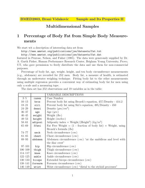
The data set has 252 observations and 19 variables as in the table:
– VARIABLE DESCRIPTIONS
3–5 casen Case Number
10–13 broz Percent body fat using Brozek’s equation, 457/Density - 414.2
18–21 siri Percent body fat using Siri’s equation, 495/Density - 450
24–29 densi Density (gm/cm 3 )
36–37 age Age (yrs )
40–45 weight Weight (lbs )
49–53 height Height (inches )
58–61 adiposi Adiposity index = Weight/(Height 2 ) (kg/m 2 )
65–69 ffwei Fat Free Weight = (1 - fraction of body fat) × Weight, using
Brozek’s formula (lbs)
74–77 neck Neck circumference (cm )
81–85 chest Chest circumference (cm )
89–93 abdomen Abdomen circumference (cm ) “at the umbilicus and level with
the iliac crest”
97–101 hip Hip circumference (cm )
106–109 thigh Thigh circumference (cm )
114–117 knee Knee circumference (cm )
122–125 ankle Ankle circumference (cm )
130–133 biceps Extended biceps circumference (cm )
138–141 forearm Forearm circumference (cm )
146–149 wrist Wrist circumference (cm ) “distal to the styloid processes”
1

Remark: There are a few misrecordings. The body densities for cases 48, 76, and 96,
for instance, each seem to have one digit in error as can be seen from the two body fat
percentage values. Also note the presence of a man (case 42) over 200 pounds in weight who
is less than 3 feet tall (the height should presumably be 69.5 inches, not 29.5 inches)! The
percent body fat estimates are truncated to zero when negative (case 182).
>> load(’C:\Courses\bmestatu\fat.dat’)
>> casen = fat(:,1);
>> broz = fat(:,2);
>> siri = fat(:,3);
>> densi = fat(:,4);
>> age = fat(:,5);
>> weight = fat(:,6);
>> height = fat(:,7);
>> adiposi = fat(:,8);
>> ffwei = fat(:,9);
>> neck = fat(:,10);
>> chest = fat(:,11);
>> abdomen = fat(:,12);
>> hip = fat(:,13);
>> thigh = fat(:,14);
>> knee = fat(:,15);
>> ankle = fat(:,16);
>> biceps = fat(:,17);
>> forearm = fat(:,18);
>> wrist = fat(:,19);
2 Covariances and Correlations
Covariances and correlations are measuring relationship between paired data sets. Let X =
(X 1 , X 2 , . . . , X n ) and Y = (Y 1 , Y 2 , . . . , Y n ) be two vectors so that components (X i , Y i ) are
matched. We can think of observing pairs (X, Y) = ((X 1 , Y 1 ), . . . , (X n , Y n )). Covariance
between paired samples X and Y is defined as
Cov(X, Y) = 1
n − 1
n∑
(X i − ¯X)(Y i − Ȳ ) = 1 [
∑ n
i=1
n − 1
X i Y i − n ¯XȲ
i=1
As in sample variances, the multiple 1/(n − 1) is sometimes replaced by 1/n.
Pearson coefficient of correlation r between samples X and Y is their covariance normalized
by their sample standard deviations,
]
.
r = Corr(X, Y) =
Cov(X, Y)
s X s Y
=
∑ ni=1
(X i − ¯X)(Y i − Ȳ )
√ ∑ni=1
(X i − ¯X) 2 × ∑ n
i=1 (Y i − Ȳ )2 .
2

where we canceled factor 1/(n − 1) in the numerator and denominator.
This is Pearson’s coefficient of correlation and it measures the strength of linear relationship
between samples X and Y.
r is dimensionless, scale invariant, and bounded, −1 ≤ r ≤ 1. If r = 1 the relationship
between X and Y is perfect linear, i.e., Y i = b 0 + b 1 X i , i = 1, . . . , n, for some constants b 0
and b 1 > 0 If the linear relationship is valid but b 1 < 0, then r = −1. If r = 0, X and Y are
uncorrelated, but not necessarily independent.
Spearman coefficient of correlation operates on the ranks of the data. Ranks are ordinal
numbers for the sorted data, the smallest observation has rank 1, next smallest 2, and so on.
In case of ties, tied observations share an averaged rank. MATLAB program (home made,
not part of MATLAB,
ranks.m find the ranks for sequences and matrices of data. For example,
>> x=rand(1,5); y=[x x(1)]
y = 0.0153 0.7468 0.4451 0.9318 0.4660 0.0153
>> ranks(y)
ans = 1.5000 5.0000 3.0000 6.0000 4.0000 1.5000
Notice that 1st and 6th observation match (by construction) and (that they are smallest.
They both have ranks 1.5 as 1+2 , and the next larger observation has rank 3.
2
Now, Spearman’s coefficient of correlation r s is defined as Pearson coefficient of correlation
among the ranks of X and Y. After some algebra,
r s = 1 −
6 ∑ d 2 i
n(n 2 − 1) ,
where d i = rank(X i ) − rank(Y i ).
Kendall’s τ is measuring association of X and Y by selecting two out of n pairs and
selecting if the pairs are concordant or discordant. The numbers of concordant N c and
discordant N d pairs among ( )
n
2 = n(n − 1)/2 possible pairs are counted. Two pairs (Xi , Y i )
and (X j , Y j ) are called concordant if (Y i −Y j )/(X i −X j ) > 0 and 1 is added to N c , discordant
if (Y i − Y j )/(X i − X j ) < 0 and 1 is added to N d .
If (Y i − Y j )/(X i − X j ) = 0 then 1/2 is added to both N c and N d and if X i = X j the
concordance is not assessed.
Then, Kendall’s τ is
τ =
N c − N d
n(n − 1)/2 .
>> X = [broz densi weight adiposi biceps];
>> varNames = {’broz’; ’densi’; ’weight’; ’adiposi’; ’biceps’};
>> varNames
>> cov(X)
>> corr(X)
3

corr(X,’type’,’Spearman’)
>> corr(X,’type’,’Kendall’)
varNames =
ans =
’broz’
’densi’
’weight’
’adiposi’
’biceps’
60.0758 -0.1458 139.6715 20.5847 11.5455
-0.1458 0.0004 -0.3323 -0.0496 -0.0280
139.6715 -0.3323 863.7227 95.1374 71.0711
20.5847 -0.0496 95.1374 13.3087 8.2266
11.5455 -0.0280 71.0711 8.2266 9.1281
ans =
ans =
ans =
1.0000 -0.9881 0.6132 0.7280 0.4930
-0.9881 1.0000 -0.5941 -0.7147 -0.4871
0.6132 -0.5941 1.0000 0.8874 0.8004
0.7280 -0.7147 0.8874 1.0000 0.7464
0.4930 -0.4871 0.8004 0.7464 1.0000
1.0000 -0.9934 0.6126 0.7290 0.4926
-0.9934 1.0000 -0.6014 -0.7224 -0.4892
0.6126 -0.6014 1.0000 0.8696 0.7822
0.7290 -0.7224 0.8696 1.0000 0.7663
0.4926 -0.4892 0.7822 0.7663 1.0000
1.0000 -0.9836 0.4356 0.5383 0.3434
-0.9836 1.0000 -0.4297 -0.5309 -0.3389
0.4356 -0.4297 1.0000 0.6880 0.5941
0.5383 -0.5309 0.6880 1.0000 0.5805
0.3434 -0.3389 0.5941 0.5805 1.0000
4

Partial coefficient of correlation
r X,Y ·Z =
r XY − r XZ r Y Z
√ √
1 − rXZ
2 1 − rY 2 Z
>> figure(1)
>> X = [broz densi weight adiposi biceps];
>> varNames = {’broz’; ’densi’; ’weight’; ’adiposi’; ’biceps’};
>> agegr = age > 55;
>> gplotmatrix(X,[],agegr,[’b’,’r’],[’x’,’o’],[],’false’);
>> text([.08 .24 .43 .66 .83], repmat(-.1,1,5), varNames, ’FontSize’,8);
>> text(repmat(-.12,1,5), [.86 .62 .41 .25 .02], varNames, ’FontSize’,8,...
’Rotation’,90);
>> figure(2)
>> %older = ismember(age,[55:max(age)])
>> parallelcoords(X, ’group’, age>55, ...
’standardize’,’on’, ’labels’,varNames)
>> set(gcf,’color’,’white’);
biceps
adiposi weight
densi
broz
40
20
1.1 0
1.05
350 1
300
250
200
150
40
20
45
40
35
30
25
0 20 40
1 1.05 1.115020025030035020 40
broz densi weight adiposi biceps
(a)
2530354045
Coordinate Value
8
6
4
2
0
−2
−4
broz densi weight adiposi biceps
(b)
0
1
Figure 1: (a) gplotmatrix for broz, densi, weight, adiposi, and biceps ; (b)
parallelcoords plot for X, by age > 55.
5

figure(3)
>> parallelcoords(X, ’group’, age>55, ...
’standardize’,’on’, ’labels’,varNames,’quantile’,0.25)
>> set(gcf,’color’,’white’);
>> figure(4)
>> andrewsplot(X, ’group’, age>55, ’standardize’,’on’)
>> set(gcf,’color’,’white’);
1.5
1
0
1
15
10
0
1
Coordinate Value
0.5
0
−0.5
f(t)
5
0
−5
−1
−10
−1.5
broz densi weight adiposi biceps
(a)
−15
0 0.2 0.4 0.6 0.8 1
t
(b)
Figure 2: (a) X by age > 55 with quantiles; (b) andrewsplot for X by age > 55
2.1 Visualizing Multivariate Data: Star Plots
The data dimension d determines the number of rays exiting from the single point; the angle
between two neighboring rays is 2π/d. The values of the data components are marked on the
rays, ith component on the ray with angle (i − 1) ∗ 2π/d, i = 1, . . . , d. This defines spokes
of the star. The star glyph connects the ends of the spokes. Thus, each spoke in a star
represents one variable, and the spoke length is proportional to the value of that variable for
that observation.
>> figure(5)
>> ind = find(age>67);
>> strind = num2str(ind);
>> h = glyphplot(X(ind,:), ’glyph’,’star’, ’varLabels’,varNames,...
’obslabels’, strind);
>> set(h(:,3),’FontSize’,8); set(gcf,’color’,’white’);
6

2.2 Chernoff Faces
The use of face representation is an interesting approach for a first look at multivariate
data which is effective in revealing rather complex relations not always visible from simple
correlations based on two-dimensional linear theories. It can be used to aid in cluster analysis,
discrimination analysis and to detect substantial changes in time series. People grew up
studying faces all the time. Small and barely measurable differences are easily detected
and evoke emotional reactions from a long catalogue buried in memory. The human mind
subconsciously operates as a high speed computer, filtering out insignificant phenomena and
focusing on the potentially important.
The feature parameters are: Variable 1-Size of face; Variable 2-Forehead/jaw relative arc
length; Variable 3-Shape of forehead; Variable 4-Shape of jaw; Variable 5-Width between
eyes; Variable 6-Vertical position of eyes; Variables 7-13- features connected with location,
separation, angle, shape and width of eyes and eyebrows; and so on.
>> figure(6)
>> ind = find(height > 74.5);
>> strind = num2str(ind);
>> h = glyphplot(X(ind,:), ’glyph’,’face’, ’varLabels’,varNames,...
’obslabels’, strind);
>> set(h(:,3),’FontSize’,10); set(gcf,’color’,’white’);
78 79 84 85
6 12 96
87 246 247 248
109 140 145
249 250 251 252
(a)
156 192 194
(b)
Figure 3: (a) Star plots for X, (b) Chernoff faces plot for X.
3 Arrythmia Example
The data set arry.dat contains the following columns: 1. Arrhythmia presence/absence, 2.
Age (years), 3. Aortic Cross Clamp Time, 4. Cardiopulminary Bypass Time, 5. ICU Time
7

6. Avg Heart Rate, and 7. Left Ventricle Ejection Fraction.
% ARRYTHMIA.M
clear all
close all
disp(’Multivariate Data:Arrythmia Example’)
%-----------------figure defaults
lw = 3;
set(0, ’DefaultAxesFontSize’, 16);
fs = 14;
msize = 5;
randn(’seed’,3)
%-------------------------------------------------------------
%1. Arrhythmia 2. Age
%3. Aortic Cross Clamp Time 4. Cardiopulminary Bypass Time 5. ICU Time
%6. Avg Heart Rate 7. Left Ventricle Ejection Fraction
arry=[...
1 68 64 126 20.25 85 81;...
1 75 111 167 13.5 50 75;...
1 69 63 94 12 74 62;...
1 88 95 145 18.25 102.5 55;...
1 75 82 132 13.25 90 78;...
1 71 14 39 10.75 88.3 80;...
1 72 80 124 12.5 88.5 56;...
1 72 85 112 14 91 70;...
1 72 97 128 14 89.5 40;...
1 82 88 128 14 77.3 33;...
1 83 49 105 14.5 79.7 65;...
1 70 87 132 14.25 71.5 50;...
1 65 98 137 15.33 89.4 38;...
1 73 47 102 13.5 86.7 62;...
1 79 108 150 16 86.7 55;...
1 70 83 122 18 74 50;...
1 73 81 120 14 68.8 55;...
1 64 0 0 14 86.2 55;...
1 81 79 157 19.5 98 80;...
1 71 81 123 22 97 70;...
1 77 107 149 17 75.8 46;...
1 53 120 137 17.5 96.5 25;...
1 66 86 109 20.75 72.8 42.5;...
1 76 61 133 17 82.5 55;...
1 75 97 149 12.67 93.8 80;...
1 74 70 147 13.42 95 80;...
1 75 72 156 8 82 70;...
1 66 98 137 15 90 35;...
0 48 102 169 18.5 76.2 59;...
0 47 81 111 12.25 70 66;...
0 62 76 126 18.5 101.4 56;...
0 71 82 130 13.62 97.6 67;...
0 48 132 224 20.5 103.2 44;...
0 85 91 124 18.17 76.3 82;...
0 54 44 89 12 87.4 65;...
8

0 69 124 210 15 81.6 60;...
0 45 105 157 14.75 96 43;...
0 53 67 119 2 94.6 64;...
0 51 23 42 17.25 74 73;...
0 70 93 148 19.25 73.2 46;...
0 69 55 109 18.5 109.3 60;...
0 76 67 101 12.25 97.4 60;...
0 61 105 185 22.5 98.4 35;...
0 69 153 233 22.5 66.4 60;...
0 50 84 113 19.5 97.3 40;...
0 70 107 142 20 82.3 59;...
0 55 116 140 13.5 70 55;...
0 72 100 148 18 80.4 53;...
0 76 77 180 23 93.2 50;...
0 77 63 109 13 87.6 39;...
0 65 78 117 16 59.2 68;...
0 57 67 103 15 79.2 70;...
0 70 107 137 19 66.8 60;...
0 69 193 487 20.75 104 60;...
0 74 90 169 14.5 94.2 50;...
0 62 71 123 13.5 66.2 65;...
0 67 72 105 19.25 76 60;...
0 64 139 196 21 77.2 18;...
0 59 55 78 12.25 88 55;...
0 44 47 77 21 107 60;...
0 51 77 138 19 99 40;...
0 48 113 120 15 82.2 60;...
0 74 0 0 12.5 79.3 63;...
0 66 80 131 20.75 88.5 60;...
0 68 94 158 18 88 30;...
0 81 90 121 14 81.4 60;...
0 70 87 120 21 81 51;...
0 76 72 108 19.5 91.8 50;...
0 66 112 163 17.75 89.8 50;...
0 61 82 129 14 76.3 60;...
0 73 46 80 20.75 80.6 50;...
0 44 87 175 15.25 97.4 65;...
0 68 102 137 13.25 71.8 71;...
0 60 99 143 18.5 85 72;...
0 73 61 91 17.5 85.6 37;...
0 69 50 98 11.67 84 55;...
0 64 63 118 13.25 97.8 40;...
0 44 75 147 18.583 111.8 60;...
0 71 51 83 16.75 102 59;...
0 73 68 122 17.833 78.2 50;...
0 55 44 78 11.5 94.8 40];
%---------------------------------------------------------------------
arryth= arry(:,1);
age=arry(:,2);
aoclati = arry(:,3);
cbt=arry(:,4);
icu = arry(:,5);
9

avehrate=arry(:,6);
lventr=arry(:,7);
%------------------
X = [age, aoclati, cbt, icu, avehrate, lventr];
varNames = {’age’,’aoclati’,’cbt’,’icu’,’avehrate’,’lventr’};
% covariances and correlations
cov(X)
corr(X)
corr(X,’type’,’Spearman’)
corr(X,’type’,’Kendall’)
corr(arryth, icu)
figure(1)
agegr = age > 60;
gplotmatrix(X,[],agegr,[’b’,’r’],[’x’,’o’],[],’false’);
print -depsc ’C:\Brani\Courses\bmestatu\Fall2007\arry1.eps’
figure(2)
older = ismember(age,[70:max(age)]);
parallelcoords(X, ’group’, older, ...
’standardize’,’on’, ’labels’,varNames)
set(gcf,’color’,’white’);
print -depsc ’C:\Brani\Courses\bmestatu\Fall2007\arry2.eps’
figure(3)
parallelcoords(X, ’group’, icu>16, ...
’standardize’,’on’, ’labels’,varNames,’quantile’,0.25)
set(gcf,’color’,’white’);
print -depsc ’C:\Brani\Courses\bmestatu\Fall2007\arry3.eps’
figure(4)
andrewsplot(X, ’group’, age>60, ’standardize’,’on’)
set(gcf,’color’,’white’);
print -depsc ’C:\Brani\Courses\bmestatu\Fall2007\arry4.eps’
figure(5)
ind = find(age>67);
strind = num2str(ind);
h = glyphplot(X(ind,:), ’glyph’,’star’, ’varLabels’,varNames,...
’obslabels’, strind);
set(h(:,3),’FontSize’,8); set(gcf,’color’,’white’);
print -depsc ’C:\Brani\Courses\bmestatu\Fall2007\arry5.eps’
figure(6)
ind = find(avehrate > 95);
strind = num2str(ind);
h = glyphplot(X(ind,:), ’glyph’,’face’, ’varLabels’,varNames,...
’obslabels’, strind);
set(h(:,3),’FontSize’,10); set(gcf,’color’,’white’);
print -depsc ’C:\Brani\Courses\bmestatu\Fall2007\arry6.eps’
10

4 Exercises and Examples
Mr Joseph Bentley, the owner of the pharmacy store wants to remove the Coke vending machine standing in
front of his store because he believes the vending machine influences the number of errors the store employees
make. More precisely, the more Coke is sold the more errors in his store is made. He provided the following
data:
errors 10 6 21 23 9 15 17 8
coke 112 100 220 250 100 200 160 100
and indeed, the coefficient of correlation is 0.9552. But we can explain this correlation because we have
complete data including the lurking variable – the number of people that passes by his store on the street,
errors 10 6 21 23 9 15 17 8
coke 112 100 220 250 100 200 160 100
people 10000 6000 17000 20000 9000 15000 14000 8000
and all the sudden the correlation disappears.
>> mederrors = [10, 6, 21, 23, 9, 15, 17, 8];
>> coke = [112, 100, 220, 250, 100, 200, 160, 100];
>> people = [10000, 6000, 17000, 20000, 9000, 15000, 14000, 8000];
>> corr(mederrors’, coke’)
ans = 0.9552
>> corr(mederrors’, people’)
ans = 0.9845
>> corr(coke’, people’)
ans = 0.9735
>> (0.9552 - 0.9845 * 0.9735)/(sqrt(1-0.9845^2)*sqrt(1-0.9735^2))
ans = -0.0801
5 Refrences
Penrose, K., Nelson, A., and Fisher, A. (1985), ”Generalized Body Composition Prediction Equation for Men
Using Simple Measurement Techniques” (abstract), Medicine and Science in Sports and Exercise, 17(2), 189.
11