Bruker Tensor 27 FT-IR & OPUS Data Collection Program - Chemistry

Bruker Tensor 27 FT-IR & OPUS Data Collection Program (V 1.1) 

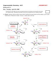
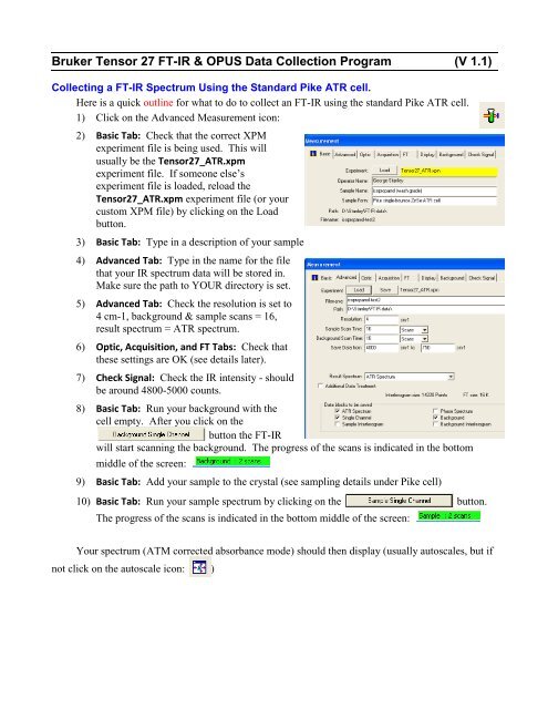
Collecting a FT-IR Spectrum Using the Standard Pike ATR cell. 

Here is a quick outline for what to do to collect an FT-IR using the standard Pike ATR cell. 

1) Click on the Advanced Measurement icon: 

2) Basic Tab: Check that the correct XPM 

experiment file is being used. This will 

usually be the Tensor27_ATR.xpm 

experiment file. If someone else’s 

experiment file is loaded, reload the 

Tensor27_ATR.xpm experiment file (or your 

custom XPM file) by clicking on the Load 

button. 

3) Basic Tab: Type in a description of your sample 

4) Advanced Tab: Type in the name for the file 

that your IR spectrum data will be stored in. 

Make sure the path to YOUR directory is set. 

5) Advanced Tab: Check the resolution is set to 

4 cm-1, background & sample scans = 16, 

result spectrum = ATR spectrum. 

6) Optic, Acquisition, and FT Tabs: Check that 

these settings are OK (see details later). 

7) Check Signal: Check the IR intensity - should 

be around 4800-5000 counts. 

8) Basic Tab: Run your background with the 

cell empty. After you click on the 

button the FT-IR 

will start scanning the background. The progress of the scans is indicated in the bottom 

middle of the screen: 

9) Basic Tab: Add your sample to the crystal (see sampling details under Pike cell) 

10) Basic Tab: Run your sample spectrum by clicking on the button. 

The progress of the scans is indicated in the bottom middle of the screen: 

Your spectrum (ATM corrected absorbance mode) should then display (usually autoscales, but if 

not click on the autoscale icon: )

Bruker Tensor 27 FT-IR Instructions (V1.1) P a g e | 2 

Table of Contents 

Tensor 27 FT-IR Introduction ....................................................................................................... 4 

Sample Cells .................................................................................................................................. 4 

Pike Miracle Single-Bounce ATR Cell (default cell) ........................................................ 4 

Liquids & solution accessory ................................................................................. 6 

Clean-up ................................................................................................................. 6 

IR Card & Salt Cell usage ................................................................................................. 7 

Switching Cells ...................................................................................................... 7 

SpectraTech solution ATR cell .......................................................................................... 8 

SpectraTech high-pressure solution ATR cell ................................................................... 8 

Tensor 27 Optical Bench ............................................................................................................... 9 

N2 purge .......................................................................................................................... 10 

Detectors – DTGS (room temp) & MCT (liquid N2 cooled) .......................................... 10 

Bruker OPUS Data Collection and Analysis Program – Intro .................................................... 11 

Login screen ..................................................................................................................... 11 

Computer Account Setup (see Bob Zinn or Greg O’Dell) .............................................. 11 

OPUS Main Window ................................................................................................................... 12 

OPUS Data Collection Details ..................................................................................................... 12 

Basic tab ........................................................................................................................... 12 

General sample info ............................................................................................. 12 

Data collection experiment/parameter file ........................................................... 12 

Advanced tab ................................................................................................................... 13 

Filename & increments ........................................................................................ 13 

Path to data directory ........................................................................................... 13 

Resolution ............................................................................................................ 14 

Background & sample scans (times) ................................................................... 15 

Data range to save ................................................................................................ 15 

Result spectrum (transmission, absorbance, ATR, etc) ....................................... 16 

ATR mode (default w/Pike ATR cell) and correction ......................................... 16 

Additional Data Treatment (not recommended) .................................................. 16 

Data blocks to be saved ....................................................................................... 17 

Optic tab ........................................................................................................................... 17 

Aperture setting ................................................................................................... 17 

Detector & scanning velocity (related) ................................................................ 18 

Sample & background gain (use auto) ................................................................. 18 

Preamp gain ......................................................................................................... 18 

Acquisition tab ................................................................................................................. 18 

Fourier Transform (FT) tab ............................................................................................. 18 

Display tab ....................................................................................................................... 18 

Background tab ................................................................................................................ 19 

Check Signal tab .............................................................................................................. 19 

Why Do You Have to Collect a Background Spectrum First? .................................................... 20 

Data Collection Outline ............................................................................................................... 21 

Data Correction & Viewing ......................................................................................................... 23 

Atmospheric Compensation: H 2 O & CO 2 ....................................................................... 23


File saves and versions .................................................................................................... 24 

Original data file version (filename.0) ................................................................. 24 

Scaling, Zooming, Spectrum color .................................................................................. 24 

Autoscale ............................................................................................................. 24 

Radar or overview window .................................................................................. 24 

Zooming spectra .................................................................................................. 25 

Peak picking ......................................................................................................... 26 

Add Annotation ................................................................................................... 28 

Color .................................................................................................................... 28 

Baseline correction .......................................................................................................... 28 

Rubber-band option ............................................................................................. 29 

Automatic option ................................................................................................. 29 

Scattering option .................................................................................................. 29 

Interactive option (danger!) ................................................................................. 29 

Straight-line & polynomial corrections ............................................................... 30 

Absorbance Transmission spectrum conversion .................................................... 30 

Multiple Spectra ............................................................................................................... 31 

Overlaid ............................................................................................................... 31 

Stacked ................................................................................................................. 31 

Interactively scaling/shifting via “Shift Curve” .................................................. 32 

Normalize spectral intensities .............................................................................. 32 

Plotting Spectra – Quick & Primitive .......................................................................................... 33 

Copy feature ..................................................................................................................... 33 

Plotting Spectra – Publication Quality (editing spectra) ............................................................. 34 

Export IR data to plotting program (Origin, SigmaPlot) ................................................. 34 

Example & Disadvantage .................................................................................... 35 

Plot as Postscript file & Edit using drawing program (CorelDraw, Illustrator) .............. 36 

Copy to clipboard problem .................................................................................. 36 

Generating Postscript file .................................................................................... 37 

Editing Postscript file with CorelDraw ................................................................ 37 

Exporting the spectrum for other applications ..................................................... 44 

Computer Access, Data copying, Backup ................................................................................... 46 

On-Campus network access (add Network Place/Location) ........................................... 46 

Off-campus access: Remote Desktop ............................................................................. 47 

Remote Desktop “danger” notice ........................................................................ 47 

Off-campus access: Virtual Private Network connection ............................................... 47


Bruker Tensor 27 FT-IR & OPUS Data Collection Program 

Tensor 27 FT-IR Introduction 

The departmental FT-IR system is a Bruker Tensor 27 system (purchased 2004) and is located in 

Choppin 702 (Figure 1). It is equipped with a room temperature DTGS detector, mid-IR source (4000 

to 400 cm -1 , and a KBr beamsplitter. Maximum resolution is 1 cm -1 . This system is free to use. The 

FT-IR software keeps a log of every user so there is no 

physical log to fill out. There is an identical Tensor 27 

FT-IR system located in Choppin 616 mainly used by 

the Stanley group for catalytic studies, but available as 

backup or for extended special FT-IR studies. 

This is a single-beam instrument so it is very 

important to generally run a background spectrum 

first!! The background will often be the empty cell, but 

for solution spectra you should run the solvent as the 

background. This is discussed in the data collection 

section. 

To use the FT-IR in Choppin 702 you must first 

Figure 1. Bruker Tensor 27 FT-IR in Choppin 702. 

ask Bob Zinn or Greg O’Dell (Choppin 100A or 100) 

to set up an account on the computer (Windows XP). They will also setup a username for you to login 

to the OPUS FT-IR data collection program. See Bob or Greg for any general computer problems you 

have with this system. You are responsible for backing up all your data on a regular basis. Network 

access instructions are provided towards the end of this document under “Computer Network Access”. 

Once you have an account you should either get Prof. George Stanley (Choppin 614, 8-3471, 

gstanley@lsu.edu) or another student in your group familiar with the FT-IR to check you out. See 

Prof. Stanley if you have questions about the optical bench, sample cell, or the FT-IR software 

program (OPUS). 

Sample Cells 

The standard sample cell in the FT-IR is a Pike Miracle single-bounce attenuated total reflectance 

(ATR) cell equipped with a ZnSe single crystal. ZnSe absorbs strongly below 650 cm -1 and data 

should not be collected below this wavenumber. The cell is shown in Figure 2(a), with close-ups of 

the top of the cell in Fig 2(b) showing the orange color of the ZnSe crystal spot upon which the sample 

lis placed. Fig. 2(c) shows the bottom of the crystal plate with the bulk of the ZnSe crystal that you do 

not see. 

(a) (b) (c) 

Figure 2. (a) Pike Miracle ATR cell. (b) Close-up of the top sample plate with the ZnSe crystal 

illuminated. The sample should cover the orange crystal surface. (c) bottom of the sample plate 

showing the rest of the ZnSe crystal that the IR beam travels through.


The ATR beam path for the cell and crystal is shown in Figure 3. The sample is placed directly 

on the small crystal spot and the arm rotated over and turned 

down to press the sample down onto the crystal face to get 

better contact. The IR beam penetrates about 60 µm into the 

sample. If your sample is extremely strongly absorbing (e.g., 

carbon nanotubes) you will not get much of an IR spectrum. 

But this ZnSe ATR cell works well for most “normal” organic 

and inorganic samples. For extremely strongly absorbing 

samples a Germanium crystal works better for ATR (we don’t 

have one), or your make a dilute KBr pellet or a thin film on 

KBr. 

The sample that is placed on the ATR crystal can be 

Figure 3. IR beam path for Pike ATR cell. 

solid, gel, liquid, or solution (non-corrosive, naturally). Since 

it will be out in the air the sample needs to be oxygen and moisture stable (for air-sensitive samples 

read on). You only need enough sample to cover the crystal surface and, if a solid, enough for the 

“crank down arm” to press the sample onto the crystal to have good contact with the crystal surface. 

The ZnSe is fairly soft, so be careful with “hard” solid samples. 

The turning handle has a built-in clutch that slips when enough downward force is applied, so 

you don’t have to worry about over tightening it. It also swings out of the way at any point above the 

crystal and has “catches” to guide it into place above the crystal surface or at the 90° away mark. If it 

gets out of alignment ask Prof. Stanley to readjust it. 

Figure 4 shows part of the sequence of events to measure a sample of plastic film (Parafilm). 

First, measure a background spectrum with nothing on the crystal (discussed under the OPUS software 

section)!! Then place the sample onto the crystal, move the lever arm over so it snaps into place above 

the crystal, then turn the top handle so the slightly concave stainless steel tip presses the sample onto 

the crystal face. 

(a) 

Figure 4. (a) Placing plastic film on crystal surface (way too big, but OK). (b) Sample depressing arm has 

been rotated over the crystal and turned down till the clutch slipped. Sample IR was then run. 

For traditional solid samples, powders work best. Although one could place a large single crystal 

of a compound directly onto the ZnSe crystal, mineral-like crystals (hard) could definitely scratch up 

the relatively soft ZnSe sampling crystal. Most organics and transition metal coordination 

compounds/complexes are softer or have similar hardness to the ZnSe. 

Gels can be smeared right onto the crystal. Be especially careful about cleaning up gooey or gellike 

samples. 

(b)


Liquid or Solution: A pure non-volatile liquid can be placed directly onto the crystal for a 

measurement. The sample pushing lever arm has a slight concave inner surface that will trap some 

liquid against the crystal so it doesn’t evaporate quite so quickly, but it is not air-tight. So it is 

generally good to lower the arm to trap the liquid against the crystal surface. 

For solutions or liquids that evaporate more quickly there is a liquid sampling accessory sitting 

on top of the FT-IR in a zip-lock bag. Figure 5 shows the sequence of photos for using this. 

(a) (b) (c) (d) 

Figure 5. (a) Three parts of the liquid sampling accessory. (b) Place disk with Teflon depression onto 

sample plate, ZnSe crystal should be centered in the middle of the hole. (c) Screw on black outer ring to 

press the Teflon portion tightly against the crystal rim. (d) Pure liquid: run background spectrum before 

adding your sample, then add sample into the Teflon depression (just a drop), cover with brass plate to 

minimize evaporation and run your sample spectrum. Solution: run background spectrum with your 

solvent in the Teflon depression (just a drop) after covering with the brass plate, then use a Q-tip or Kimwip 

to soak up the solvent and give it some time to dry. Then add your sample solution, cover with brass plate 

to minimize evaporation and run your spectrum. Aqueous solutions are OK. NO strong acids or bases. 

Although the Teflon disk makes a pretty good seal against the base plate, there may be a bit of 

leakage underneath (keep this in mind when cleaning up). 

This cell is NOT very sensitive for samples in solution. You need fairly concentrated samples 

(around 0.2 M) to get a semi-reasonable spectrum. Some dilute sample solution spectra are shown 

later under the data collection and scan time section – they are not very good. Those of you that 

experiment with solutions with this Pike single-bounce ATR cell, please provide me feedback and I 

will include that here. 

You can also use this liquid sampling accessory for solids as the conical Teflon section is useful 

for directing the solid sample onto the crystal. You would not use the brass cap for a solid sample. 

Instead, crank the arm-press tip down onto the solid to make sure it is pressed firmly against the crystal 

surface. 

CLEAN-UP: It is very important to clean the cell surface well after you are done. There should 

be a bottle of isopropyl alcohol, kimwips, and Q-tips to the right of the optical bench. Please refill or 

replace these from your own labs as they are used up. 

Acetone is OK for cleaning the cell surface BUT it may take the paint off the IR optical bench 

and eat away at some of the plastics (note damage on computer case!!). Do NOT FORGET to clean 

the bottom of the steel lever arm that pushes down on your sample!! If you use the liquid sampling 

setup shown in Fig. 5, make sure that you clean the stainless-steel/Teflon disk well.


Salt Plate/Pellet/IR card Holder: This is shown in Figure 6 and is 

sitting on the shelf on top of the FT-IR optical bench. The pellet/plate 

holder is inserted (Fig. 6, bottom) but can be removed. This can allow you 

to insert other disposable IR-card type sample holders such as screen, KBr, 

or polyethylene film (Fig. 7). 

Figure 7. IR screen (gooey samples), KBr real crystal, and polyethylene 

sample cards. 

Figure 6. (top) IR card-salt 

plate holder and separate 

pellet holder. 

(bottom) assembled. 

To switch cells one just needs remove the existing cell by pressing the cell release lever located 

at the right front of the base locking plate (Figure 8), tilt the front of the cell up and out of the front 

locking plate, then remove the cell. 

The new cell is inserted with the cell base plate 

electronics connection pointed to the back of the FT-IR 

cell locking system. Fit the back portion of the cell in 

first with the front of the cell tilted up, then press down 

and lock into place. 

Most of the newer cells for the Tensor 27 have base 

plates with electronics that uniquely identifies the cell to 

the spectrometer. There is an automatic accessory 

recognition (AAR) feature that can pre-load reference 

background spectra for a cell, set data collection 

parameters, and enable simple sample collection. This 

Figure 8. Cell base plate unlocking lever. 

AAR feature is not currently activated, but may be in the 

future. See Prof. Stanley and later sections in OPUS for more information.


SpectraTech Circle ATR Solution cell: This cell is shown in Figure 9 and can be obtained 

from Prof. Stanley. Although it is an older technology it works well for solutions and small scale 

reactions. The sample cell has a 4.0 cm long cylindrical ZnSe crystal rod. The IR beam bounces 

(a) 

(b) 

Figure 9. (a) SpectraTech Circle micro-ATR solution cell. (b) close-up of removable ATR microcell. 

through the rod resulting in multiple sampling points throughout the solution. The solution volume 

needed is about 0.5 mL. The sample concentration in solution should be at least 50 mM. 100-200 mM 

sample concentrations will give good spectra. There originally was a thin metal plate to cover the top 

to limit solution evaporation. This cover is missing, but we can rig up some plastic to do the same job. 

Due to the longer IR beam pathlength through the crystal rod the more sensitive liquid nitrogen 

(LN 2 ) MCT (mercury-cadmium-telluride) IR detector needs to be used. The MCT detector is stored in 

Choppin 616 with the other Tensor system and can be obtained from Prof. Stanley. Instructions for 

using or filling the MCT detector with LN 2 are given in the next section on the FT-IR optical bench. 

SpectraTech High Pressure/Temp Circle ATR Solution Reaction Cell: This is a 40 mL Parr 

stainless steel mini-autoclave with a hole drilled through it for a ZnSe ATR crystal rod. It can handle 

gas pressures up to 1,500 psig (100 atm) and temperatures up to 200°C. A schematic drawing and 

photos are shown in Figure 10. 

(a) (b) (c) 

Figure 10. (a) Schematic drawing of high pressure circle rxn cell. (b) Photo of cell bottom mounted in holder. (c) Photo of 

cell bottom along with the stirrer head piece, valves, thermocouple, and electronic pressure transducer. 

This circle rxn cell is operated by a Parr 4850 autoclave process 

controller shown in Figure 11, which can control and track the 

temperature, stirring rate, and the pressure of the autoclave, along with 

the pressure of an external high pressure gas reservoir. A manual 

pressure regulator is available with the external gas reservoir to deliver 

a constant pressure gas or gas mixture to the IR cell. Prof. Stanley’s 

group has used this cell for studying hydroformylation catalysis by 

mono- and dinuclear rhodium complexes. For their studies that focus 

Figure 11. Parr controller for the 

high pressure circle rxn cell.


on the metal-carbonyl band region (2200-1700 cm -1 , typically strong absorbances) metal complex 

concentrations of at least 30-50 mM were needed to get decent spectra of just the metal-carbonyl 

region. 

As with the regular solution circle ATR cell discussed above (very similar ATR technologies), 

the high sensitivity MCT detector must be used. 

For more information on this system, see Prof. Stanley. 

Air-Sensitive Samples: Collecting the FT-IR of oxygen or moisture-sensitive samples can be 

quite a challenge. Air-sensitive solution IR’s can be fairly easily collected using the high-pressure 

circle rxn ATR cell discussed above. A septum replaces the head assembly for ambient solution data. 

A nujol mull of an air-sensitive solid sample prepared in a glove box can be put between two 

KBr plates and into a zip lock bag for transfer out of the glove box and to the FT-IR for use in the KBr 

plate sample holder. The diffusion of O 2 or moisture into the center of the mull sandwiched between 

the two plates is generally slow enough to obtain good FT-IR spectra on the central portion of the 

plates. 

For other air-sensitive sampling methods and special procedures see Prof. Stanley. 

Tensor 27 Optical Bench 

The Tensor 27 FT-IR optical bench has no external controls and is operated completely (aside 

from the power switch on the back) from the computer system. The optical path of the bench and 

major components are shown in Figure 12. 

Figure 12. Schematic of Tensor 27 optical bench, IR beam path, and major components. A = mid-IR 

source, B = aperature wheel, C = filter wheel, D = exit port (not used), E = beamsplitter, F = switch mirror, 

G = sample compartment window (KBr), G’ = optional window (not present), H = sample holder/cell, I = 

detector (DTGS standard).


The optical bench should be continuously purged with a slow flow of house nitrogen to keep 

moisture and CO 2 out of the source, interferometer, and detector compartments. Do NOT turn the N 2 

off!! The inside of the Pike ATR cell is also connected to the N 2 flow to further improve the signal-tonoise. 

Note that the Pike cell has sleeves that extend out to fit over the source and detector holes. 

Make sure that these sleeves are flush against each side of the sample compartment to maintain the N 2 

atmosphere inside the cell and spectrometer. 

The main N 2 shut-off/on valve is on the 

wall next to the door and shown in Figure 

13(a). The smaller circular valve controls the 

flow rate to the FT-IR. The N 2 flow rate is 

shown on the flow meter between the computer 

and optical bench (Fig. 13(b)). This flow meter 

is not good at measuring low flow rates and 

will be replaced at some point. The flow only 

needs to be enough to just get the ball moving a 

bit unless one needs a short-time fast purge. 

(a) (b) 

Figure 13. (a) Main N 2 valve with blue swing handle. Round 

valve with label for FT-IR N 2 flow. (b) Flow meter. 

Detectors: The standard IR detector is the room temperature DTGS (deuterated tri-glycine 

sulfate) detector. This is fine for 98% of typical samples run. We also have a high sensitivity liquid 

nitrogen (LN 2 ) cooled MCT (mercury-cadmium-telluride) detector for use with the more IR-beam 

absorbing cells mentioned previously or special samples. 

For highly demanding applications like the circle ATR solution cells one needs to make use of 

the high sensitivity broad-band MCT detector stored in Choppin 616. The MCT detector is ~10 times 

more sensitive than the DTGS detector! See Prof. Stanley for instructions on how to switch the DTGS 

and MCT detectors. 

This detector has a small red dewar for the LN 2 . To use the MCT detector the red dewar needs to 

be filled with LN 2 using the plastic funnel with the 4” metal tube attached and the white polystyrene 

spacer shown in Figure 14. 

Filling the MCT dewar takes a fair bit of time 

(~ 5-8 min) due to the time needed to cool down the 

funnel and dewar. Add the LN 2 slowly and 

minimize the spilling onto the FT-IR. Often right 

near the end of the cool down/filling process some 

of the LN 2 will “geyser” up out of the dewar, 

sometimes blowing the funnel out as well. This is 

normal and signifies that one is near the end of the 

dewar cooling stabilization process. 

Usually before this geysering event the MCT 

detector has cooled down enough that the system 

reads it as functional. The FT-IR optical bench will 

“beep” and the STATUS light on the top right-hand Figure 14. Dewar schematic and photo of MCT detector. 

side will change from red to green. 

After filling the dewar remove the funnel and replace the small filler plug (which fits loosely) 

into the top of the FT-IR. The MCT detector is now ready to use. A filled dewar will last around 4-6 

hours. 

Each Tensor 27 FT-IR optical bench and computer is hooked up to an uninterruptable power 

supply (UPS) to protect it from power outages and surges.


Bruker OPUS Data Collection and Analysis FT-IR Software Program 

OPUS (OPtical User Software) is the Bruker data collection and analysis 

program for the Tensor 27 FT-IR. Currently version 4.2 is installed on the computer 

in 702. Version 5.0 is installed on the computer in 616. Both are essentially identical 

in operation. We will be upgrading to version 6.5 in the near future. This section will 

then be updated as needed. 

We have permission from Bruker to load OPUS on lab and office computers to 

view and analyze data away from the FT-IR. See Prof. Stanley for a CD. A full on-line manual is 

available via the HELP menu. Prof. Stanley has a hard copy in his office. 

After starting OPUS the first thing you are presented with is the login screen shown below (left). 

The User ID’s are listed in order of creation, not alphabetically. Find your name from the list (right 

screen), type in your password, and double check that the Assigned Workspace is as shown below. 

Then click on the Login button. It is possible to create your own workspace, but this is only for 

advanced users that are very familiar with the software. 

Bob Zinn or Greg O’Dell (Chemistry computer support personnel) need to setup an OPUS 

account for you. Make sure you let them know your faculty advisor’s name so they can add that to the 

Windows user information. OPUS requires at least Power User privileges (or higher) in case you are 

setting it up on your own system. You should also have a user directory on the D: drive of the 

computer where you should store all your data. 

Remember to always backup your data!! 

If you forget your password (Windows or OPUS) please see Bob, Greg, or Prof. Stanley to reset 

it. Typing in the wrong password too many times for OPUS will lock the account. 

After the Login screen there is a welcoming screen that 

listed information about OPUS (version #, license code, #, 

etc). Click the OK button to proceed.


The main OPUS window is shown below. Key icons and areas are labeled. 

Advanced Data collection – FT-IR settings 

Auto scale spectrum 

Baseline correction 

Peak picking 

File and 

window use 

list 

IR Spectrum Window 

Window sizes can be adjusted by positioning the mouse cursor on the 

window boarders. The mouse pointer will change to twin vertical lines 

with arrows pointing both directions – you can then left-click and drag to 

change the window size 

IR Spectrum “Radar” Window 

Window tabs Data collection info FT-IR status 

(yellow or red – 

contact Prof. Stanley) 

Data Collection Details/Settings: 

The data collection menus are opened by clicking on the icon shown or by selecting the Measure 

menu, then Advanced Measurement. This will open up 

the Measurement window with a number of tabs giving 

details on various aspects of the FT-IR, data collection, 

and FT processing. 

The Basic tab lists the Experiment file being used 

to input the default FT-IR parameters for data collection. 

This file is called Tensor27_ATR.xpm. The file is stored 

in C:\Program Files\OPUS\XPM. If you see a different 

filename it is probably because the previous user 

loaded their own custom XPM file. 

When you setup a special experiment and change a 

number of parameters for data collection you can save 

the experiment as an XPM file to load again when 

needed. It is best to store this in your own data directory,


but some students store theirs in the program 

directory (try not to). 

If you see some other experiment file loaded 

you should reload the Tensor27_ATR.xpm file by 

clicking on the Load button next to Experiment and 

directing the program to the Tensor27_ATR.xpm file 

in the C:\Program Files\OPUS\XPM directory (screen 

to the right). This XPM file is setup especially for 

the Pike ATR accessory. 

If you are running salt plates (e.g., NaCl or 

KBr) pick that experimental file or just change the 

Result Spectrum (discussed below) under the 

Advanced tab to absorbance or transmission (not 

ATR spectrum). 

The FT-IR does have Automatic Accessory Recognition (AAR) and I will experiment with this 

when we get the new OPUS v6.5 software installed and update these instructions. This feature 

recognizes the cell being used and loads the appropriate data collection parameters and background 

reference spectra. So you would directly add your sample and run the spectrum (no initial background 

needed). It is NOT active right now. 

The Sample Name and Sample Form fields are text messages to identify your sample, phase 

(liquid, solid, film, etc.), and cell being used. 

Next, click on the Advanced tab to bring up that screen. Although this screen is labeled 

“advanced” it has basic critical fields that you need to fill in. Importantly, this is the screen where you 

specify the Filename: that your spectrum and 

data will be stored into. Use an informative 

filename. OPUS will add a number as the 

file extension, starting with 0 (your original 

data – do NOT delete). It will auto-increment 

the extension # if you run a new spectrum 

and keep the same filename. Example: 

polystyrene.0 

polystyrene.1 

polystyrene.2 

The Path: also needs to be checked and 

set to where you are storing your data!! This 

should be D:\username + any subdirectory 

name where you are storing your FT-IR data. 

Note that the user directory for the PREVIOUS user may be present!! So it is very important that you 

reset this path to YOUR data directory!! 

Clicking on the button to the right of the Path: input line will bring up the file/directory 

selection window so you can direct the program to your data directory. 

This “advanced” screen has almost all the common settings that you may want to adjust: 

resolution, # of background & sample scans, saved data range, type of spectrum (transmittance, 

absorbance), and data blocks that you want to save in the spectrum file. Descriptions of these key 

settings are discussed below.


Resolution: This is the instrument’s spectral resolution in units of wavenumbers (cm 1 ). The 

normal setting is 4 cm 1 . Signal to noise in a spectrum is proportional to the square root of the 

acquisition time (# of scans). Doubling the resolution requires a four times higher acquisition time to 

achieve the same Signal-to-Noise ratio. Polystyrene film samples run on the Pike ATR cell at various 

instrument resolutions are shown below (with an enlargement of the 1600 cm 1 region shown to the 

right). These were not corrected for ATR (discussed later), but illustrate the resolution effect well. 

The times to collect 8 scans at the 10 kHz scan speed (standard for the DTGS detector) are listed with 

each spectrum. 

The gross features of all 5 spectra are the same. Sharp peaks that lie close together, however, are 

adversely affected at the larger (lower) resolution settings. Note in the expanded view that the peak at 

1600.5 cm 1 and its shoulder at 1582.5 cm 1 (which are 18.0 cm 1 apart) are well resolved in the 2 

and 4 cm 1 resolution spectra, start losing definition in the 8 cm 1 spectra, and are pretty much 

smoothed together in the 16 cm 1 spectrum. 

There are no differences between the 4 and 1 cm 1 spectra that justify the increased data 

collection time required at 1 cm 1 (or higher) resolution. Typically, one only uses the high resolution 

settings for gas phase spectra (we skipped the 0.5 cm 1 resolution option on this system since almost 

all our IR work is solution or solid phase). Solution and solid-state samples, for the most part, have 

broader peaks that certainly do not get any narrower by increasing the resolution setting on the FT-IR. 

If you do not have close lying sharp peaks and need faster collection times, the 8 or 16 cm 1 resolution 

options may be very good, but I would recommend running test spectra at 4 cm 1 resolution to make 

sure no important peak information is lost at the lower resolution settings. 

The increased “noise” in the 1 and 2 cm 1 spectra arises in part from the non-perfect substraction 

of the water vapor peaks from the background spectrum (the lower resolution settings broaden these 

sharp peaks leading to better subtraction), but mostly from the fact that we ran the same # of scans for 

each resolution. Remember that doubling the resolution requires a four times higher acquisition time 

to achieve the same Signal-to-Noise ratio.


Background and Sample Scan Times: We typically specify this with the # of scans (time in 

minutes is the other option). One almost always runs the same number of background scans as sample 

scans, so these should generally be the same. An unequal number of background and sample scans can 

lead to poor background subtraction (dramatically increased H 2 O and CO 2 atmospheric peaks, positive 

or negative going depending on conditions). 

16 scans is the current default for the Tensor27_ATR.xpm experiment file. For most “normal” 

concentration samples (pure liquids or solids) you will pretty much get an acceptable spectrum after 

only 1 scan. Since a scan at 4 cm 1 resolution and 10 kHz scan speed only takes about a second, you 

can afford to collect 16 scans to get good signal to noise. Remember that signal to noise (S/N) in a 

spectrum is proportional to the square root of the acquisition time (# of scans). So if the S/N is not 

good enough, increase the # of scans by a power of 2 (e.g., 16 to 256). 

For example, the effects of scan 

time (4 cm 1 resolution, 10 kHz scan 

speed) for a dilute 10 mM solution of 

acetone in water are shown to the right 

using the Pike ATR cell (not good for 

dilute solutions!). 

It is clear that the 8 and 64 scan 

spectra are not really showing anything. I 

would say that the 256 scan spectrum is 

starting to see the intense carbonyl stretch 

and maybe a few of the other strong 

bands. These bands are somewhat clearer 

in the 4,096 scan spectrum, but hardly 

what I would call good. 

The spectra shown include an 

atmospheric H 2 O/CO 2 and aqueous 

correction (details later). This cleaned up 

the 256 and 4096 scan spectra a fair bit, 

but had little effect on the 8 and 64 scan 

IR’s. 

So having a concentrated enough 

sample is very important. Doing a lot of 

scans will not pull up a dilute sample 

from the noise or solvent subtraction 

artifacts unless you get lucky or have 

very strong bands. 

Save Data Range: This represents the wavenumber range that will be saved and displayed for 

the spectrum. If you are using the Pike cell the ZnSe crystal absorbs most or all of the data below 650 

cm 1 . If you are using a KBr cell you can go down to 400 cm 1 . The FT-IR is equipped with KBr 

beamsplitter so no data is available below 400 cm 1 . There isn’t much data above 4000 cm-1 and this 

is the typically upper limit. 

Note that the FT-IR interferometer physically scans from 8000 to 0 cm 1 , but we only save a 

portion of that range.


Result Spectrum: This should be set on ATR Spectrum 

if you are using the Pike single-bounce ATR cell (or another 

ATR cell). The ATR mode records the IR spectrum in 

absorbance mode (peaks go “up” like an NMR spectrum) and 

applies an intensity correction to the spectrum. If you prefer 

transmission mode (peaks go “down”) you can easily change 

the ATR absorbance spectrum into transmission using the AB 

TR conversion option under the Manipulate menu, or the 

icon on the screen. 

The penetration of IR radiation into the sample from the ATR crystal is wavelength dependent, 

with higher wavelengths getting less penetration and lower intensities. The ATR intensity correction 

partially compensates for this and is illustrated in the three 

polystyrene spectra shown to the right. 

The top spectrum is a polystyrene film recorded on 

the Pike ATR cell in transmission mode, then converted to 

absorbance (8 scans, 4 cm 1 resolution, 10 kHz). The 

second spectrum was collected the same way but using the 

ATR mode setting. The third spectrum is the internal 

polystyrene standard (no Pike ATR cell) collected in 

absorbance mode. 

Note that the C-H region (around 3000 cm 1 ) is 

considerably more intense than in the non-ATR corrected 

top spectrum. The ATR correction shown in the middle 

spectrum doesn’t completely match the “correct” 

intensities shown in the bottom spectrum, but is a good 

compromise. Keep these intensity differences in mind 

when comparing your spectrum collected on the ATR cell 

to literature or database spectra that may be from a KBr 

sample (non-ATR). 

Other result spectrum settings include transmission (100% to 0%, peaks point “down”), 

absorbance, Kubelka Munk (corrections for diffuse reflectance spectra), reflectance, and photoacoustic 

(PAS) spectra. If you have removed the Pike ATR cell to use the direct salt-plate/IR card cell then you 

should change Result Spectrum to absorbance or transmission. Note that most of these corrections can 

be applied to a spectrum collected in one of the other modes (Convert Spectra option under 

Manipulate menu). 

Additional Data Treatment: Generally not used at this point. I recommend doing any data 

treatments after basic data collection so you have a better idea of what impact you are having on the 

spectrum.


Data Blocks to be Saved: We typically save the spectrum, single channel (raw sample 

spectrum), and background. The spectrum (or trace) is the result of an automatic subtraction of the 

background spectrum from the single channel 

spectrum (sample + background). I strongly 

recommend saving both the single channel and 

background as they are both needed for any 

subsequent atmospheric (H 2 O/CO 2 ) data correction. If you want to be careful save the sample and 

background interferograms. These represent the raw data. All this information is saved in the file and 

the program can extract what you specify (more under data analysis & atmospheric correction). 

Optic: Normally you don’t have to change anything here, but you should always check it to 

make sure some previous user didn’t screw things up by changing things and then saving the new 

settings over the Tensor27_ATR.xpm 

experiment file. 

I will only discuss a few of the settings 

that you might change under some 

circumstances. 

Aperture Setting: Also known as the 

Jacquinot stop (J-Stop). This is an iris or 

aperture that is placed in the path of the IR 

beam between the source and the 

interferometer. The default setting should be 

wide open – 6 mm. Note that on the Tensor 

system in 702 aperture values up to 12 mm are 

listed, but 6 mm is the true largest setting. Do 

not set it larger than 6 mm. 

The purpose of the aperature is to select out only the center-most part of the IR beam where the 

IR radiation is the most parallel, or least divergent, as it enters the interferometer. This improves the 

resolution of the spectrometer for very narrow peaks. Naturally, this is only important for gas phase 

samples that have very narrow, highly resolved peaks. If one increases the resolution of the instrument 

to 1 cm -1 , for example, OPUS will flag the Optic tab with a blue information tag and highlight the 6 

mm aperture setting with a yellow background. This is the programs way of informing you that this 

setting should be changed to a smaller value to match your higher resolution. As you make the 

aperture smaller you are cutting down the intensity of the IR beam, so you need to watch the intensity 

under the Check Signal tab. The FT tab will also get an information mark to adjust some of those 

settings as well. 

One practical use for the aperture is to reduce the intensity of the IR beam when using the highly 

sensitive MCT detector. The maximum # of counts of IR radiation that the detector can handle before 

producing “distortions” in the collected spectrum ~26,000 counts (given as a negative # under Check 

Signal). Above this the detector is starting to saturate out. While many samples that demand use of the 

MCT detector will also drop the beam intensity enough, you may run into some samples where the 

MCT detector energy reading too high. In these cases one can close down the aperture to internally cut 

down the IR beam intensity to an acceptable level (under 25,000 counts). 

If you change the aperture, please remember to reset it back to the 6 mm settings for the next 

user! Unfortunately, some of the parameter settings get carried over to the next user if they are 

changed (despite loading in a fresh XPM parameter file).


Detector Setting and Scanner Velocity: The normal detector is the room temperature DTGS 

and the recommended interferometer scan velocity for this detector is 10 kHz. Do NOT change these 

unless you use the MCT detector!! If you need to use the liquid nitrogen cooled MCT broad-band 

detector the system will flag the detector setting to change. For the MCT detector one should use the 

20 kHz velocity setting. 

Sample and Background Gain: This sets the gain on the FT-IR internal electronics. Raising 

the gain increases the signal from the detector, but it also increases the background noise by a similar 

amount. There is little reason, therefore, to ever set the gain higher than 1 or automatic. If you need 

more signal to noise either collect more scans or use the MCT detector. 

Preamp Gain: should be set to A. Do not change. 

Acquisition: Normally you don’t have to change anything here, but you should always check it 

to make sure some previous user didn’t screw things up by changing things and then saving the new 

settings over the Tensor27_ATR.xpm experiment file. All the settings should be as shown below. 

FT (Fourier Transform) tab: Normally you don’t have to change anything here, but you 

should always check it to make sure some previous user didn’t screw things up by changing things and 

then saving the new settings over the Tensor27_ATR.xpm experiment file. All the settings should be 

as shown below. See on-line information or the manual for details on the settings. 

Display: Normally you don’t have to change anything here. The initial display will show 

wavenumbers from 4000 to 400 cm -1 . This window typically tracks with what is set for the data 

collection save range (4000 to 700 cm-1). The spectrum display window auto-adjusts to the spectrum 

range saved.


Background: Normally this is not used since you should usually collect a fresh background 

spectrum for each sample. BUT, if you have a saved background from a previous run that you want to 

load that can be done here. 

To load a background from a previous run you 

first need to open and load the spectrum file in 

question. Look carefully at the file and window pane 

on the left-hand side of the OPUS display. An 

example is shown below. 

There are four boxes of data stored in the spectrum file. The first (highlighted in red) is the final 

sample spectrum or trace (TR). The next box represents the “raw” sample or single channel (S-SC) 

spectrum. The third box represents the reference or background single channel spectrum (R-SC). The 

last box is the History file that tracks anything you do to your original spectrum. 

To load the background from this file you can 

take your mouse cursor and left click on the R-SC box 

and, while holding the mouse button down, drag it and 

drop it into the white box under the Load Background 

button. You will now see the display to your right. 

Now you can click the “Load Background” 

button to put this background single channel spectrum 

into the FT-IR background memory slot. This 

background will then be used when you collect the 

next sample spectrum. If you actively collect another 

background it will replace this loaded background. 

Check Signal: This is the other tab that you SHOULD check before every run!! This lets you 

know how much IR radiation the detector is receiving. Too low and you won’t be able to record a 

spectrum or it will be filled with noise and no signal. 

There are 3 types of displays available: interferogram, spectrum, and ADC count – all shown 

below. 

For the interferogram and spectrum screens the IR intensity is shown at the top of the screen as 

the Amplitude. The amplitude is listed as a negative number and the absolute value can vary from just 

above 3 to a high of about 18,400 counts (DTGS detector, standard settings). 

Without the Pike ATR cell the IR intensity for the FT-IR system in Choppin 702 should be 

around 18,300 counts. With the Pike ATR cell in place and a good N 2 purged optical bench you 

should see an intensity of 4,400 to 5,050. If you see a significantly lower value, please contact Prof.


Stanley. Adding sample should drop the IR beam intensity as some is now being absorbed by the 

sample. 

Why Do You Have to Collect a Background Spectrum First? 

Our FT-IR systems are single beam instruments. Air contains water vapor and CO 2 that are 

considerable absorbers of IR radiation. Water, in particular, has a host of sharp peaks in the gas phase 

and even in our air conditioned building the humidity level is still significant. The KBr window that 

isolated the source and interferometer compartments along with some of the other optics have organic 

coatings that also add to the background. Shown below are the single channel background (reference) 

specrum (magenta) and “raw” single channel sample spectra (green) for polystyrene film. Note that 

the computer converts the interferogram to a transmission-type spectrum. The “sample” spectrum, as 

you can see, includes all the very significant background peaks, some of which I have labeled. The 

FT-IR internal computer substracts these to generate the final sample spectrum (trace) shown at the 

bottom of the page. 

CO 2 

H 2 O 

organic 

coatings 

The twin CO 2 peaks at 2361 and 

2339 cm 1 very commonly 

appear in your final sample 

spectrum. 

Do not mis-interpret these as part 

of your sample. 

H 2 O


Collecting a FT-IR Spectrum Using the Standard Pike ATR cell. 

Here is an outline for what to do to collect an FT-IR using the standard Pike ATR cell. 

11) Click on the Advanced Measurement icon: 

12) Basic Tab: Check that the correct XPM experiment file is being used. This will usually be 

the Tensor27_ATR.xpm experiment file. If someone else’s experiment file is loaded, reload 

the Tensor27_ATR.xpm experiment file (or your custom XPM file) by clicking on the Load 

button. 

13) Basic Tab: Type in a description of your sample 

14) Advanced Tab: Type in the name for the file that your IR spectrum data will be stored in. 

Make sure the path to YOUR directory is set. 

15) Advanced Tab: Check the resolution is set to 4 cm-1, background & sample scans = 16, 

result spectrum = ATR spectrum. 

16) Optic, Acquisition, and FT Tabs: Check that these settings are OK (see previous section). 

17) Check Signal: Check the IR intensity - should be around 4800-5000 counts.


18) Basic Tab: Run your background with the cell empty. After you click on the 

button the FT-IR will start scanning the background. The progress 

of the scans is indicated in the bottom middle of the screen: 

19) Basic Tab: Add your sample to the crystal (see sampling details under Pike cell) 

20) Basic Tab: Run your sample spectrum by clicking on the button. 

The progress of the scans is indicated in the bottom middle of the screen: 

Your spectrum (ATM corrected absorbance mode) then displays (usually autoscales, but if not 

click on the autoscale icon: )


Manipulating/Correcting your Spectrum 

Atmospheric Compensation (H 2 O/CO 2 ): Just by chance in the previous FT-IR there is a fair 

bit of negative going water and CO 2 absorbances present. This occurred because I was playing with 

the Pike ATR cell (removed and replaced several times) which let more water vapor and CO 2 into the 

cell itself. I then ran the background spectrum, BUT waited over 30 mins before running the sample. 

This allowed 30 mins of N 2 purging through the cell that reduced the amount of water vapor and CO 2 

present when I finally ran the sample spectrum. Thus the original background spectrum that was 

subtracted from the sample + background spectrum had more water vapor and CO 2 present giving rise 

to negative intensity peaks (down-going) in the absorbance spectrum. 

To do an Atmospheric Correction that should minimize the water and CO 2 bands, click on the 

Manipulate menu (shown to the right), then click on Atmospheric Compensation. That will bring up 

the empty screen (below left). 

You now should left mouse click on and drag the sample single channel 

block (S-SC box) from the file display window and drop it into the top white 

box on the Atmospheric Compensation window. Do the same thing with the 

single channel reference block (R-SC) into the bottom section (screen, top 

right). Then click “Calculate”. Here is the spectrum before (left) and after 

(right) the correction:


There is also an option to apply a correction for aqueous solutions. 

Also note that after doing the atmospheric correction the file icon now shows a red page on top of 

the normal cyan color: 

This indicates that the file has not been saved since the last spectral manipulation/correction. You 

can easily reverse what you did by clicking on the undo icon: 

The two quickest ways to save the spectrum file are right click on the red page indicator shown 

above, then select the Save File option (below left), or click on the file save icon, . Either of these 

brings up the final File Save option box (below right). 

After saving the file, the red file marker goes away. 

IMPORTANT NOTE: When you save a file after doing some sort of spectra correction OPUS 

creates a new version of the file with the modified spectrum by incrementing the numerical extension 

on the filename. So your original data is always stored in filename.0. The file with the highest 

numerical extension is the most recent version that contains all the data manipulations that you have 

done up to that point. 

Scaling/Zooming/Shifting/Peak Picking/Color: Scaling and zooming the FT-IR spectrum is 

fairly straightforward. 

If the spectrum does not load with the maximum X and Y expansion, click on the autoscale icon 

to expand the spectrum. This is a very valuable button and is the quickest way to get you back to 

the full spectrum. 

The bottom window running across the main spectrum window shows a smaller, squished 

spectrum. This is the “radar” or overview window and can be used to adjust the main spectrum 

window. It is a bit tricky to use but good for fine adjustments. If you are working on a big enough 

display, I suggest doubling the size of this window vertically by clicking on the upper border and 

dragging it up to take away some room from the main spectrum window. 

The “problem” with the autoscale button (function) is that it maximizes the vertical scale of the 

spectrum so the largest peak extends from bottom to top (absorbance type spectrum). This is typically 

too much if you want to do peak picking (next section) and list the picked peak frequencies on the top 

of the spectrum. The best way to add a bit more white space on the top or bottom of the spectrum is to 

use the overview window and increase the extent of the space around the spectrum.


This is done by moving your mouse cursor to the top or bottom border of the overview window. 

When it changes to this pointer ( , or the single line version) you can left click your mouse and drag 

the white space around the spectrum to decrease it (make the spectrum in the main window more 

vertically expanded) or to increase it, which as the effect of reducing the vertical extent of the spectrum 

in the main window. If you move the mouse pointer just a bit higher it will change to a horizontal 

double line with up and down single arrows. This is the cursor that allows you to change the size of 

the overview window itself. Although the screen captures do not grab the mouse cursor the two views 

below show the effect of dragging the overview window white space up to make more room at the top 

of the main spectrum window. You can do the same thing on the bottom (which I did for the right side 

view) if want to add a bit more white space there as well. 

There is no button currently in the program that will increase or decrease the vertical scale in 

small increments. So practice with the overview window scaling features. 

Zooming is pretty simple. Just right click on the main spectrum screen 

to bring up the menu shown to the right. Select zoom in and the menu will 

disappear and be replaced by vertical and horizontal dashed cursor tracking 

lines. Click to select the first defining point for your expansion region, then 

click the opposite corner point to define a square or rectangular expansion 

region. This does NOT immediately zoom the region selected, rather the 

dashed zoom box is now floating and will follow your cursor to allow you to 

position it more accurately around the part of the spectrum that you want to 

expand. Once you have it positioned correctly left click again to invoke the zoom. See images below 

showing the selection and the zoomed region on the next page.


Notice the overview pane on the bottom of the screen. The zoomed region is shown with the 

white box. You can grab this white box with the mouse and move it around or resize the boundaries to 

change the zoom level!! By moving the box around you can scroll through the spectrum in a zoomed 

mode and fairly easily change the zoom level by changing the size of the white box in the overview 

window. That is why it is good to expand this window somewhat. 

Once again, the quickest way back to the full spectrum is to click on the autoscale icon . 

Peak Picking is also quite easy and is best done using the full 

spectrum. Click on the peak picking icon or select Peak Picking 

from the Evaluate menu. This will bring up the peak picking screen 

shown to the right. Interactive mode is the best option, clicking on that 

modifies the main spectrum window as shown below.

Bruker Tensor 27 FT-IR Instructions (V1.1) P a g e | 27 

By sliding the Threshold square up (more sensitive, more peaks picked) or down (less sensitive) 

you can determine what peaks are picked for labeling with the wavenumber. Note that the top 

numbers do NOT always appear on the display at this stage. What does always appear are the small 

vertical tick marks above peaks that are picked. 

Once you have adjusted the threshold to get most of the peaks you want click the Store button 

and you will exit the peak picking mode and return to the main display with the peaks labeled with 

their wavenumber. At this point a new peaks data block is added to your spectrum file over in the file 

display window. This is shown below. 

Right-clicking on this Peaks block and selecting the “Show Peak List” option will open a new 

display window with the peak pick list (shown below).


If you want to mark a specific peak with a wavenumber label all you have to do is right click at 

the point where you want it annotated and select the “Add Annotation” option. This does not 

automatically pick the peak maximum, so it is best if you are zoomed in when you do this. This adds 

an arrow pointing at the point where you right clicked the spectrum 

and the wavenumber with a ridiculous number of digits after the 

decimal point. Right clicking on this annotation and selecting 

“Properties” allows you to edit the number and reduce the number of 

digits after the decimal point (one is sufficient). Left clicking on the 

annotation allows you to move it around. 

I haven’t figured out how to increase the size of the font used as 

yet (but see later section on publication/talk/dissertation improved 

display options). 

The color of the spectrum and peak picking marks/labels can be 

easily changed two different ways. The first is by left mouse clicking on the appropriate data block in 

the file window. Each time you click the color of that object will rotate around a pre-defined color 

pallet. 

Want to more directly set a specific pre-defined color? Then right 

click directly on the spectrum and select the “Set Color” option. That 

will bring up the following screen with the colors available. Click on 

the color you want. This also works for the peak picking labels/tick 

marks. It does NOT work for annotations. 

Baseline Correction: Samples that have sloped baselines can be “leveled out” using the 

Baseline Correction function under the Manipulation menu or via this icon . The following 

spectrum is a good candidate for baseline correction (automatic or manual).


Invoking the Baseline Correction brings up the screen shown below (left). The Select Method 

tab gives the choices shown on 

the middle screen. The default 

rubberband option and 64 

baseline points typically works 

well. Clicking on the Correct 

button starts the automatic 

baseline correction procedure and 

gives the spectrum shown below 

in blue. 

The scattering correction is 

more “aggressive” at pulling 

down the minima between peaks 

to the baseline. The automatic 

correction using the scattering 

option (64 points) is shown below 

in red. 

To me the scattering option 

tries too hard at dragging peak 

minima down to the baseline. But 

I have to admit that it looks more 

like a classical IR spectrum. It is 

easy to try both. I would include 

which baseline option you use in 

your experimental procedure. 

The interactive option should 

only be used when you want more 

control over the baseline correction 

or if the automatic correction doesn’t work well. A key factor in doing the interactive baseline 

correction is to decide what part of the spectrum should be on the baseline!! The “dips” between 

closely spaced peaks in the 1400 cm 1 and lower region often do NOT touch the baseline due to 

overlap. Forcing them “down” via the interactive manual procedure when they should not be on the 

baseline could be considered “wrong” and improper data manipulation. So you need to be very careful 

when doing the manual interactive baseline procedure and not get carried away. 

The interactive manual baseline routine changes the main spectrum window to give two spectra 

as shown below. The top window (blue spectrum in this case) is the one for double clicking on the 

baseline to defining the points that the spectrum will be pinned to for defining the baseline. A baseline 

point is defined when and where you left double mouse click. The points are NOT locked onto the 

spectrum and can be moved around once created. Double-clicking on an existing point will delete it. 

The figure below shows all the points I defined. The bottom spectrum represents the “corrected” 

spectrum based on the baseline points that you have added and is updated interactively as you add 

baseline points. Once you are happy, click on Store and you will be returned to the main spectrum 

window with the baseline corrected spectrum.


I typically use the straight-line option, but the polynomial correction would be used for a baseline 

that has a lot of curvature in it. But you should experiment and see what works best for your spectrum. 

Absorbance to Transmission Conversion: If you like your spectrum presented as transmission 

(downward pointing IR peaks) then use the AB TR function under Manipulate menu or via the 

icon. The menu screen that opens up is shown to the right. The automatic mode generally works 

fine so all you have to do is click on convert. I converted the absorbance spectrum shown above 

(baseline corrected) to give the following transmission spectrum.


Displaying Multiple Spectra: The default mode when you load (or collect) more than one 

spectrum is overlay as shown below. I adjusted the spectrum colors to give reasonable contrast. 

Clicking on the Display menu function Stacked or the stack plot icon 

generates the perhaps 

more usable screen shown below. Clicking on the stacked icon again returns one to overlaid mode. 

In overlay mode the display is scaled to the biggest peak in one of the spectra and there is no 

obvious display option to vertically expand one (or more) of the other spectra if they are less intense to 

see those peaks better. There are two ways around this.


The easiest method of interactively scaling overlaid spectra is to right click on the appropriate 

spectrum and select the “Shift Curve” option. There are three sub-options to shift curve: whole curve, 

top, and bottom. The top option allows you to click on one of the peaks and drag it (holding the left 

mouse button down) up or down. This, in effect, can individually scale the intensity of one of the 

overlaid (or stack plot) spectra. This is a “local” intensity change that is not saved with the spectrum. 

The trace can be easily returned to the original intensity using the “Shift Curve – reset” option. Note 

that the master XY rescale button will NOT sense any local intensity changes made using the Shift 

Curve options, that is it will behave as if you have not changed the intensity of the spectrum using the 

shift curve option. However, the Y rescale option does keep track of the shift curve intensity changes. 

You can also shift the bottom of the spectrum or shift the entire spectrum up or down with the other 

shift options. 

The other method is to normalize all the spectra intensities using the Normalize function under 

the Manipulate menu or the normalize icon . That brings up the 

screen to the right. 

By default this screen will only have one of the spectra listed, 

unless you have all the spectral files highlighted in the spectrum 

window. Otherwise, you need to click and drag the trace block of 

each of the other spectra over into the “Files for Normalization” 

window (which I have done). The Min-Max method generally works 

fine and what I used for this example. It normalizes each spectrum 

so the minimum absorbance is 0 and the max absorbance of the 

biggest peak in each is equal to 2. See the on-line help for more 

details on the other options. Normalizing all 5 spectra generated the 

overlaid display shown below. 

You should naturally NOT use normalized spectra for doing any quantitative calculations or 

comparisons between spectra. OPUS will save the normalized spectra with a new version #.

Transmittance [%] 

50 60 70 80 90 100 


Plotting Your Spectrum – Quick and Primitive (for your notes or advisor): Just click on the 

Quick print icon 

or select Quick Print from the Print menu. This works well for individual 

spectra (with or without peak picking) and overlaid spectra (with or without peak picking). It does 

NOT currently work for stacked spectra (next version of OPUS may fix this). I have extra ink 

cartridges for the inkjet printer in my office. Let me know when they need replacing. 

A primitive (but effective) work around for getting a plot of your stacked plots is to press the 

Print Screen button on the computer (upper right side of keyboard). This does a bitmap screen capture 

and places it into the Clipboard. You can then open a new Word file and paste the image into it. Word 

has a cropping tool that you can use to trim the full screen capture to just what you want. This is how I 

got almost all the images into this document. Print the Word file and/or save it for future use. 

You can also Copy the spectrum to the Windows Clipboard and paste it into Word or most other 

applications. An example is shown below. 

3500 

3000 

2500 

2000 

Wavenumber cm-1 

1500 

1000 

This is especially nice if you are keeping an electronic notebook. This is not a bitmap, but rather 

a vector graphics file and is quite compact. It can be edited using the Word drawing editing features 

and this will be discussed more later.


Nice Spectra – Publication, Dissertation, Powerpoint Presentations: There are several 

methods to take the basic plot(s) provided by OPUS and upgrade them to something suitable for 

publication (paper or dissertation) or presentation (e.g., Powerpoint). All of these involve some work 

and editing. DO NOT SCAN IN YOUR SPECTRUM. All methods below generate vector graphics 

files that have high resolution, small sizes, and don’t become pixilated as you make them bigger. 

Export Data as ASCII X,Y Data File – Replot with Plotting Program. Exporting the data from 

OPUS as an X,Y data file is quite simple and shown below. With your spectrum on the screen click on 

File menu, then Save File As. This will bring up the first screen shown below left. Change the path to 

your directory (middle screen), then type in the file name and use a TXT extension. You can only 

export ONE spectrum at a time. 

Then go to the Mode tab and click on Data Point Table as your file format. The Data Point 

Table tab shows the format for your data. The number format refers to the # listed after the decimal 

point. You don’t need 5 decimal points for the wavenumber or intensity, but I usually leave it set at 5. 

The screen below shows the text data file created (parafilm.txt) and that file opened with Notepad 

showing the X,Y data pairing as wavenumbers and intensity.


You can then import this X,Y text file into a plotting program such as Origin or Sigmaplot, re-plot the 

data and fine tune the graph to your satisfaction. I used the SigmaPlot (9.0) program to import some 

FT-IR data and a sample plot with ChemDrawings added is shown below (cut and pasted into Word). 

1.4 

Test FT-IR - Xylene/Hexane Mixture 

CH 3 

1.2 

1.0 

H 3 C 

H 2 

C 

H 2 

C 

C 

H 2 

CH 3 

C 

H 2 

Absorbance 

0.8 

0.6 

CH 3 

0.4 

0.2 

0.0 

3000 

2500 

2000 

1500 

1000 

Wavenumbers (cm -1 ) 

The major disadvantage to this method is losing the peak picking labels and not being able to 

highlight important peaks/data. While journals do not usually want peak picking wavenumber figure 

labels in the main body of a paper, they are very good for dissertations or supplementary material. 

Most plotting programs can handle stack and multiple plots, but fine tuning can be a pain.


Plot Data as Postscript File, Import into Vector Drawing Program & Edit. This method 

works equally well for any spectrum (IR, NMR, etc) that you can save as a postscript file. I have 

loaded CorelDraw, a vector drawing and editing program, onto both FT-IR computers. A student 

edition of the CorelDraw X3 program suite that includes PhotoPaint (photo & bitmap editing program) 

and CorelCapture (screen capturing utility) costs about $110 at the bookstore. Adobe Illustrator is 

another good (but more expensive) vector drawing/editing program. 

Below is an example of what you can do to “enhance” an FT-IR using one of these drawing 

programs. Time involved using CorelDraw? About 30 mins (once you know what you are doing). 

It is quite easy to color specific peaks by changing the line color, thickness, or, with a little more 

effort, using a background fill (solid or transparent) as shown above (or a mixture of both). 

ChemDraw structures are also easily added. This is also probably the easiest way to get a nice stacked 

plot of several spectra. You can easily rescale the intensity and position of the spectra to get a good 

view. See page 37 for more details on editing with CorelDraw. 

Why not use the Copy function or Print to Clipboard? Copy and Print to clipboard are two 

options that capture a Windows Metagraphic File (WMF), which is a vector graphics file of what you 

are seeing on the screen. The problem I have found with this and OPUS is that the resolution of what 

you capture seems to vary in a way that I don’t fully understand with both operating system (Windows 

XP vs. Vista) and screen resolution. Sometimes you get a fairly high resolution capture of your 

spectrum, sometimes it looks terrible. Printing your spectrum to a postscript file and then importing 

that file into the drawing program produces a higher resolution spectrum curve consistently.


Generating a Postscript File. We have created postscript file printers for both of the FT-IR 

computers labeled Postscript to File. In OPUS go to File Print Setup and select this as your 

printer and make sure the Landscape mode is chosen. See Prof. Stanley if you want to set this up on 

your lab or notebook computer, not all postscript drivers work equally well for this (we are using the 

Xerox Phaser 7400 postscript driver). 

Then do a Quick Print of your spectrum (and peak picking if you want). Only do one spectrum at 

a time!! If you have multiple spectra displayed, un-display them by right clicking the trace (or ATR) 

display data block in the file window and select the “Remove from Display” option. This does NOT 

delete the spectrum, just changes its color so it doesn’t appear on the screen. 

After clicking the Quick Print icon, a file save 

box will pop up similar to that shown to the right. You 

need to input the drive and directory where the file will 

be saved. This is NOT the standard file save dialog 

box that lets you select the directory to save the file, so 

it is important that you know the drive, your directory 

name, and in what subdirectory you want to save it. I 

suggest using .ps as your file extension – both Adobe 

Acrobat and CorelDraw automatically recognize this as a postscript file. 

Using CorelDraw to Enhance your Plot. The procedure shown below will work 

for almost any postscript file of any spectrum (NMR, IR, mass spec, X-ray powder 

diffraction, etc). The following procedure does not go into excessive detail. Please see 

Prof. Stanley for more information on using CorelDraw if you have questions. 

Start CorelDraw, select “New” from the welcome screen, 

and switch the page orientation into landscape mode by 

selecting Layout, then Switch Page Orientation from the menu 

that drops down (figure shown to right). 

Select File Import and select your Postscript file 

for import. If the file has a .ps extension CorelDraw should 

recognize it as a Postscript file and ask if you want to import 

text as text (fonts) or curves. Select text and next. A screen will 

then pop up with suggested font substitutions. Just click OK to 

proceed. The CorelDraw cursor will then change to a corner. 

You can now click on the screen to import the spectrum. 

The spectrum will import in a vertical orientation, so you need to rotate it by -90.0° to get it into 

the proper “horizontal” orientation. Use the Rotate menu box and type in -90.0° (boxed in red below) 

and carriage return. Reposition the spectrum (click and drag) so it is oriented nicely in the page 

definition space (page outline).


The imported spectrum and associated text is all grouped together as one object. You need to 

ungroup the imported figure so you can edit the various sub-pieces (spectrum, fonts, colors, etc.). 

Click on the spectrum to select it, then click on the ungroup icon on the main menu, near the rotate 

box. This ungroup icon is boxed in green on the previous figure. Next to it is an ungroup all icon, 

which in this case will do the same thing. 

Click away from the spectrum to unselect it. Now you can click on any of the spectrum object to 

edit them. The main screen should look something like that shown below (I did not display peak 

picking on this spectrum, so they didn’t print). 

An important point at this juncture is to realize that the spectrum trace has also been un-grouped 

into a 1000+ separate data points connected by lines. If you click on the spectrum trace you will see 

that one data point is selected. Be careful that you do NOT move any of the data points! That would 

be considered modifying your data, which could be an ethical violation. It is OK to change the 

intensity of the entire spectrum so long as you are not trying to make quantitative comparisons between 

different samples/spectra. 

At this point we can carefully work with the spectrum to select some peaks to highlight them by 

selectively re-coloring the line and/or changing the line thickness for emphasis. For example, I can use 

the mouse to click and select a box around one of the peaks to pick all the data points and lines 

comprising that peak. Right clicking on one of the colors on the right side color pallet (more available 

by clicking on the expand arrow at the bottom) will change the line color. Left mouse clicking 

changes fill or text/font colors. But at this point we have no closed objects so there is no fill color to 

change.


The figure below shows one of the peaks selected and the line color (right click) changed to red. 

The line thickness can now be changed for this 

red line by clicking on the fountain pen nib (Outline 

Tool) on the left-hand vertical set of icons, then 

selecting the fountain pen nib icon again. This brings 

up the Outline Pen screen shown above. One can 

now change the line thickness to whatever value 

desired. I suggest clicking on the Scale with Image 

box as well. This will rescale the line thickness if you 

change the size of the image within CorelDraw. The 

figure to the right shows the effect of increasing the 

line thickness from the imported value of 0.199 

points to 1.5 points. 

Generally, however, I think it is better to make 

the entire spectrum the same line thickness and 

highlight peaks of interest with different colors or 

using a fill color (discussed next). 

To use a fill color you should copy (control-C) 

and paste (control-V) the selected peak to make 

another version to convert into a filled area. When 

you paste a copied object into CorelDraw it pastes it into the exact same position so it looks like 

nothing has been done!! But a new copy has been pasted and you can verify this by using the arrow 

keys to move the object a bit so you can see the new object. Alternatively you can do a control-D key 

sequence, which will duplicate the object and automatically translate it a bit so you can see the new 

duplicate more clearly.


IMPORTANT Point: Remember that your original spectrum trace is still composed of 

thousands of individual data points. So it is critically important that you move this new copied peak to 

a location where it is NOT overlapping with the original spectrum. If you click somewhere else on the 

page the new object (peak) will be deselected and if it is overlapping with the original spectrum trace 

you will not be able to select one or the other cleanly. 

To this copied or duplicate peak you want to now click on the Arrange main menu category, then 

choose Close Path Closest Nodes with Straight Lines (next figure). 

That generates the closed object shown to the right (shifted away 

from the original spectrum), which was initially hollow. 

This has now been converted into a single object with a 

closed shape. 

I then left clicked on the red color to fill it with red and right 

clicked on the no outline color (white box with an X through it at the 

top of the color scale) to remove the outline. 

An easy way to get a lightly shaded color for this filled peak is 

to use the transparency tool/option, shown below. 

Selecting the “cup” icon changes the main menu and creates a 

new group of icons & selections shown below.


I changed the first box to “Uniform”, which activated the other items to the right of it. The box 

with 50 in it refers to the amount of transparency applied to the object. The higher the number the 

lighter and more transparent it is. There is a slider control to the left of this, but typing in a number is 

more accurate. Transparency not only lightens the color but allows objects below it to show through. 

As shown in the spectrum example on page 36 this can also be used to blend colors to show 

overlapping regions. 

At this point I recommend moving the filled transparent peak off to the side and proceeding with 

any other peaks you want to fill and highlight. 

Once you are done, you should carefully select the entire spectrum (watch out that you do NOT 

select any of the surrounding lines!) and group it together as a single object. If you are pretty sure that 

you do NOT want to do any more peak abstracting the other option is to select the entire spectrum and 

click on Arrange Combine. This will convert all the separate points (nodes) into a connected 

curve (a single object). BUT, the Combine command will NOT allow different line colors within a 

spectrum. So if you have changed the line color of some of the peaks use the Group function. 

Once the spectrum is grouped together or combined, you can move the filled peaks back and 

overlay them onto the appropriate areas on the spectrum. Then do another group command. 

To get fine object movement control (needed to overlay your filled peaks on your original 

spectrum) using the arrow keys you should change the Ruler Nudge option under Tools Options 

Document Rulers. Then change the Nudge, Super nudge, and micro nudge values as 

shown below. Holding down the control key while pressing an arrow key will move an object by 

micro amounts. Holding down the shift key while pressing an arrow key will move the object macro 

amounts. After changing these values, make them the default by clicking on Tools Save 

Settings as Default.


Text Editing: Text is imported as text and can easily be selected and the fonts, size, and weight 

(italics) changed. I personally like Arial bold with a font size of about 14 for the wavenumber scale. 

Superscripts and subscripts can be specified using the text edit command, BUT the 

super- and subscripts generated this way look way too small. I, therefore, recommend 

using the Shape Tool button (shown to the right) that is right below the select button on 

the left-hand side menu. Clicking on the text using the Shape Tool places small boxes to 

the left of each character and places two corner arrow objects, one pointing down and the other on the 

far right pointing to the left. 

The small empty squares to the left of each character allow them to be selected and individually 

modified and moved using the mouse or arrow keys. This allows you to fine tune the superscripting or 

subscript size and location (just make sure you are consistent). Holding down the shift key and left 

clicking the two small boxes for the -1 selects both characters for editing. I decreased the font size 

using the top menu Font boxes and then while they were still selected used the up arrow key to move 

them up and to the left a bit to give the following result: 

The arrow object to the far left will spread out (or condense) the spacing of the text. The down 

arrow at the front of the text will interactively change the line spacing between two or more lines of 

text. 

You can also color and rotate text. The outline and fill colors for text can be different, which is 

good for light colored text (example below). The outline weight or heaviness can also be easily 

adjusted. 

Multiple Spectra: When importing multiple spectra to do a stack or overlay plot, import each in 

separately and make sure you edit that trace away from the others and then group it together as one 

object once you are done. Also make sure that each is on the same wavenumber scale!! 

The reason that you can’t import in an overlayed set of traces all at once is that there is almost no 

way to select one trace for modification when they are overlapping in any significant way. Once you 

ungroup the traces each data point is separate. If you are happy with the colors and do not want to do 

anything fancy, it is easy to select all the traces and change their line weights without affecting their 

colors. But you won’t be able to move one trace relative to the others. 

I do not know why OPUS won’t print or export stacked plots well, hopefully the new version 

(6.5) will handle this better. 

Rescaling Spectra: Be careful rescaling spectra in CorelDraw. If you change the vertical scale 

remember that the absorbance or transmittance scale will no longer be accurate (unless you scale that 

as well). This is especially important for the horizontal scale & axis. If you want to show an expanded 

portion of your spectrum with a wavenumber scale, I suggest expanding it in OPUS, printing to a 

separate Postscript file, then importing into CorelDraw as a separate spectrum that you edit, group, and 

position on your main spectrum as an insert.


Two Examples: A simple single ATR absorption spectrum of acetone printed from OPUS as a 

Postscript file, imported into CorelDraw, and “fixed up” is shown below. Time involved: 10 mins 

(includes a phone call “interruption”). 

The “fancy” overlaid and stack plot shown earlier. This took about 30 mins (including the 

ChemDrawings).

ATR Units 

0.0 0.5 1.0 1.5 2.0 2.5 3.0 3.5 

3412.93 

3004.35 

2967.37 

2924.36 

1748.37 

1712.20 

1420.44 

1359.49 

1220.43 

1092.23 

901.98 

785.11 


Exporting from CorelDraw to Word or PowerPoint: Although you can sometimes copy and 

paste from CorelDraw directly to Word (or other Office apps), it is better if you export your spectrum 

or drawing as a Portable Network Graphics (PNG) file and import that into Word or Powerpoint. 

Although a PNG file is a bitmap it has some very nice features such as anti-aliasing (to smooth lines), 

compact size (for a bitmap), and 24 bit color depth. TIFF bitmaps are much larger than PNG bitmaps. 

Shown below is the acetone spectrum directly copied and pasted from CorelDraw into this Word 

document with the exported PNG spectrum file right below. Which one do you think is better? 

Acetone (wash grade, Pike ATR cell) 

CorelDraw 

copy & paste 

3500 

3000 

2500 2000 

Wavenumber (cm-1 

) 

1500 

1000 

CorelDraw 

PNG export


The other BIG advantage of using a PNG graphics file of your spectrum or drawing is that it 

looks great in PowerPoint due to the anti-aliasing effect that smoothes out lines, removing the “jaggy” 

look. Yet another potential advantage is that the PNG graphic can be created with a transparent 

background. This is great if you have a lightly colored background on your PowerPoint slides that you 

want to show through the image. A screen capture of a PowerPoint slide with a light blue gradated 

background and the PNG graphics file of the acetone spectrum is shown below. 

Of course, you may not always want a transparent background and that is one of the options 

when you export the PNG file from CorelDraw (along with resolution, color depth, etc). 

One “problem” with PNG graphic files is that Adobe Acrobat does not generally do a good job of 

converting these into the PDF file format. However, the PDF file export option in the Microsoft Office 

2007 suite does an excellent job of translating PNG graphics files to PDF. Note that if you are using 

Office 2007 the PDF file creator is not initially present (due to a lawsuit by Adobe). But you can 

easily download and install the PDF file creation module for Office from their web site. I strongly 

recommend doing this. The Office PDF file creation function is accessed under File Save As 

PDF or XPS. This PDF file was generated using this Office feature.


Copying and Backing up Your Data 

You can use a USB flash drive or external hard disk drive to copy and backup all your data. I 

have put a USB extension cord attached to the front of the Dell computer to make it easier to plug in 

your storage device. Use Windows Explorer to copy your entire directory over to your storage device, 

or just the files in question. 

Network file transfers. You can also directly link into the FT-IR computer and transfer files 

over the network to your lab computer (or notebook computer). The procedure varies depending on 

whether you are on campus or not (on campus is easiest) and the computer/operating system. The 

instructions below are for Windows XP or Vista computers. I don’t know much about Mac’s, for help 

see Les Butler or our computer support personnel. 

The FT-IR Computer in Choppin 702 has two names assigned to it. The internal Windows 

netbios name is CH702-FTIR. The automatic LSU network (netreg) registration name tied to your 

PAWS ID is gstanley-7.lsu.edu. These will change if we shift the computer to the LSU Active 

Directory. 

On-Campus Access. If you are accessing the computer disk drive from on campus you should 

use the CH702-FTIR name (not case sensitive). 

Windows XP: 

1) Go to Start My Network Places and click on Add a network place. This starts the 

add network place wizard. Click next to continue. 

2) Select “Choose another network location”, click next. 

3) Type in the name of the computer in question. In this case it will be: 

\\ch702-ftir\d\user-directory-name 

Note that the computer must have file and printer sharing enabled and disk drive sharing 

setup (d in this case). 

4) You should now get a Windows Login screen. You need to type in your username for that 

computer and the password. Click on “remember my password” if you want to by-pass this 

screen in the future (if you change your password this login screen will reappear). 

5) If the username and password is correct you will now get a screen with a suggested name for 

this new network place. Modify the name to be clear and informative to you. Click next and 

then Finish. This will open by default a file view window to the drive/folder in question and 

create a new Network Place link/shortcut under Network Places. You can copy this to your 

desktop if you intend on accessing it a lot. 

Windows Vista: 

1) Go to Start Computer, this opens up the screen showing all the disk drives and 

network paths to other computers. 

2) Right mouse click on the blank area of the screen in the main window. Select “Add Network 

Location” from the menu that appears. This initiates the Add Network Location wizard. 

3) Choose “Custom Network Location” and type in the name of the computer in question. In 

this case it will be: 

\\ch702-ftir\d\user-directory-name 

Just as for Windows XP, the computer you are liking into (and yours!) must have file and 

printer sharing enabled and disk drive sharing setup (d in this case).


4) You should now get a Windows Login screen. You need to type in your username for that 

computer and the password. Click on “remember my password” if you want to by-pass this 

screen in the future (if you change your password this login screen will reappear). 

5) If the username and password is correct you will now get a screen with a suggested name for 

this new network place. Modify the name to be clear and informative to you. Click next and 

then Finish. This will open by default a file view window to the drive/folder in question and 

create a new Network Location link/shortcut under Computer. You can copy this to your 

desktop if you intend on accessing it a lot. 

Adding a Network Place or Location is analogous to Mapping a Network Drive. The advantage 

to defining a Network Place in Windows XP is that the password appears to be firmly stored. When 

you Map a network drive you assign an open drive letter, but my XP computer often forgot the account 

password needed to re-link into the drive mapped computer on a reboot. Vista is much better about 

remembering passwords for Mapped Network Drives, so there is little difference between the two. 

Both mapped network drives and network locations appear under Computer in Windows Vista. 

For Windows XP network places are listed under My Network Places (usually below My Computer in 

the file explorer listing). Once you have these defined you can readily copy files back and forth 

between the two computers. 

Off-Campus Access. If you are accessing the computer from OFF-campus the easiest way to 

access your data is to use the Remote Desktop program and the gstanley-7.lsu.edu computer name 

(Windows XP or Vista). For those of you that have not used Remote Desktop it is a very powerful 

program that allows you to login to a remote computer and work on that computer and have access to 

all its resources, files, and programs as if you are actually there working on the computer. It works 

through the Windows Firewall, but you need to setup the remote computer to accept Remote Desktop 

sessions (Remote tab located under My Computer properties in Windows XP, or Computer, then 

System Properties, Remote tab in Windows Vista). 

When establishing a Remote Desktop link to a computer you need to specify via the Options 

selection (at least the first time you setup the connection) that you want to share resources between the 

computers and the type of internet connection being used (the Experience tab). Sharing drives is the 

default option and allows one to copy files between both computers. 

WARNING: a Windows computer can only have one user logged in at a time, either directly or 

via Remote Desktop. When you login to a computer using Remote Desktop you will get a message if 

another user is logged in and a warning that if you proceed you will abort that users session and kick 

them off. If you are the one logged in locally and never logged off, that is fine. But if someone else is 

logged in you do NOT want to kick them off unless you have their permission or know that they are 

not actively using the computer (i.e., they forgot to logoff and are not doing anything on the computer). 

You also have to have administrator privileges to do this (I believe). When you are done, remember to 

LOGOUT of your account. Remote Desktop will then automatically close. If you simply exit from 

the Remote Desktop program you will still be logged onto the computer in question and any programs 

will continue running. 

The more complicated way to access the files on a campus Windows computer from off-campus 

is to establish a virtual private network (VPN) connection. IF the campus computer in question is 

either on Active Directory -OR- part of the LSU workgroup you can then map a drive or setup a 

network place/location. LSU has upgraded their network security to NOT allow Windows File and 

Printer sharing functions (drive mapping, network places) from off-campus except via a VPN 

connection and to computers that are part of the Active Directory or LSU workgroup. See Prof. 

Stanley or the computer support personnel (Greg O’Dell, Bob Zinn) for more information on this.

Bruker Tensor 27 FT-IR & OPUS Data Collection Program - Chemistry

Create successful ePaper yourself

Delete template?

Save as template?