Localized Amplification of Seismic Waves and Correlation with ...

Bulletin of the Seismological Society of America, Vol. 86, No. 1B, pp. $209--$230, February 1996 

Localized Amplification of Seismic Waves and Correlation with Damage 

due to the Northridge Earthquake: Evidence for Focusing in Santa Monica 

by S. Gao, H. Liu, P. M. Davis, and L. Knopoff 

Abstract The analysis of seismograms from 32 aftershocks recorded by 98 seismic 

stations installed after the Northridge earthquake in the San Fernando Valley, 

the Santa Monica Mountains, and Santa Monica, California, indicates that the enhanced 

damage in Santa Monica is explained in the main by focusing due to a lens 

structure at a depth of several kilometers beneath the surface and having a finite 

lateral extent. The diagnosis was made from the observation of late-arriving S phases 

with large amplitudes, localized in the zones of large damage. The azimuths and 

angles of incidence of the seismic rays that give rise to the greatest focusing effects 

correspond to radiation that would have emerged from the lower part of the rupture 

surface of the mainshock. Thus the focusing and, hence, the large damage in Santa 

Monica were highly dependent on the location of the Northridge event, and an earthquake 

of similar size, located as little as one source dimension away, would not be 

likely to repeat this pattern. We show from coda wave analysis that the influence of 

surface geology as well as site effects on damage in Santa Monica is significantly 

smaller than are the focusing effects. 

Introduction 

During the 17 January 1994 Mw = 6.7, depth = 19 km 

Northridge earthquake (USGS and SCEC, 1994), Sherman 

Oaks and mid-Santa Monica experienced much greater 

damage than neighboring regions at similar distances from 

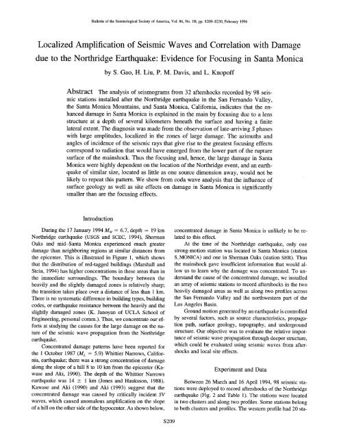
the epicenter. This is illustrated in Figure 1, which shows 

that the distribution of red-tagged buildings (Marshall and 

Stein, 1994) has higher concentrations in these areas than in 

the immediate surroundings. The boundary between the 

heavily and the slightly damaged zones is relatively sharp; 

the transition takes place over a distance of less than 1 km. 

There is no systematic difference in building types, building 

codes, or earthquake resistance between the heavily and the 

slightly damaged zones (K. Janoyan of UCLA School of 

Engineering, personal comm.). Thus, we concentrate our efforts 

at studying the causes for the large damage on the nature 

of the seismic wave propagation from the Northridge 

earthquake. 

Concentrated damage patterns have been reported for 

the 1 October 1987 (ML = 5.9) Whittier Narrows, California, 

earthquake; there was a strong concentration of damage 

along the slope of a hill 8 to 10 km from the epicenter (Kawase 

and Aki, 1990). The depth of the Whittier Narrows 

earthquake was 14 + 1 km (Jones and Hanksson, 1988). 

Kawase and Aki (1990) and Aki (1993) suggest that the 

concentrated damage was caused by critically incident SV 

waves, which caused anomalous amplification on the slope 

of a hill on the other side of the hypocenter. As shown below, 

concentrated damage in Santa Monica is unlikely to be related 

to this effect. 

At the time of the Northridge earthquake, only one 

strong-motion station was located in Santa Monica (station 

S_MONICA) and one in Sherman Oaks (station SHR). Thus 

the mainshock gave insufficient information that would allow 

us to learn why the damage was concentrated. To understand 

the cause of the concentrated damage, we installed 

an array of seismic stations to record aftershocks in the two 

heavily damaged areas as well as along two profiles across 

the San Fernando Valley and the northwestern part of the 

Los Angeles Basin. 

Ground motion generated by an earthquake is controlled 

by several factors, such as source characteristics, propagation 

path, surface geology, topography, and underground 

structure. Our objective was to evaluate the relative importance 

of seismic wave propagation through deeper structure, 

which could be evaluated using seismic waves from aftershocks 

and local site effects. 

Experiment and Data 

Between 26 March and 16 April 1994, 98 seismic stations 

were deployed to record aftershocks of the Northridge 

earthquake (Fig. 2 and Table 1). The stations were located 

in two clusters and along two profiles. Some stations belong 

to both clusters and profiles. The western profile had 20 sta- 

$209

$210 S. Gao, H. Liu, P. M. Davis, and L. Knopoff 

34°10 ' 

\ • 

• i[ • • 

/= m 

i • m ! 

-:'(.n ,, , n , 

i ""-.-.. i m • tim 

34°12 ' 

34°06 ' 

34 ° 09' 

34°08 ' 

34°07 , 

,, • -- a-,.. ;'~-Im~ _ 

/ • ... -'.,. 

: S "' . .5. 

i 

• / • # 

i 

' 

• 

"krh 

, 13 1 2 

-118°28 ' -118°26 ' 

34°00 ' 

34°02 ' 

I 

km 

o i 

• • j/ 

ii ./ l/ 

m %. i II • ,~ i 

% I m ./ m 

"-. i ",~ I1~" • /"+all 

34 ° 01' 

-118°36 ' 

-118°30 ' -118°24 ' -118°30 ' -118°28 ' 

Figure 1. Distribution of red-tagged buildings and topography. The coordinates of 

the red-tagged buildings are from Marshall and Stein (1994). Diagrams on the right are 

enlargements of the inset areas. 

tions, and the eastern one, 16 stations. Both profiles were 

about 35-km long, along lines with strike 165 °, and traversed 

the San Fernando Valley, Santa Monica Mountains, and the 

northwestem part of the Los Angeles Basin. The northern 

cluster of 36 stations was centered in Sherman Oaks in a 7 

by 7 km area; the distance and azimuth of the center of the 

Sherman Oaks cluster (station B16) from the epicenter are 

about 11 km and 133 °. The southern cluster of 29 stations 

was centered in Santa Monica in a 4 by 3 km area; the distance 

and azimuth of this cluster (station F10) from the epicenter 

are about 21 km and 168 °. 

All stations were equipped with Reftek digital recorders. 

A trigger mode was used to record relatively strong events. 

The length of each seismogram was 80 sec, including 20 sec 

of pretriggering time. The long pretriggering time proved to 

be useful, because the S waves from some events were the 

triggering signals at some stations, and the long pretriggering 

time saved the first arrival. The sampling rate was set at 

125 samples per second, and the data format was 16 or 32 

bit, depending on the type of Reftek recorder (72A-02, 72A- 

06, 72A-07, or 72A-08). About half of the stations were 

equipped with GPS receivers and thus had relatively accurate 

times and locations. The clocks of stations without GPS receivers 

were corrected every week during station service using 

external GPS clocks, and the locations for those stations 

were obtained from USGS 1:24,000 series topographic maps. 

There were 75 stations equipped with L28 4.5-Hz sensors, 

8 with L22 2.0-Hz sensors, and 15 with L4C 1-Hz 

sensors. The amplitudes of the seismograms from the sensors 

were standardized to the uniform response function of an 

L28. There were no obvious relations between the corrected 

amplitude and sensor type, as shown below. The station locations 

and sensor types are listed in Table 1 and shown in 

Figure 2. 

Five of the 98 stations could not be used because (1) of 

malfunctioning amplifiers, (2) data could not be recovered

Localized Amplification of Seismic Waves and Correlation with Damage due to the Northridge Earthquake $211 

34°10 ' 

\ 

t 

; ci30 

¢ BIS~ D070 

i 

.......... ~ cls 0 

34 ° 12' 

34°06 ' 

34 ° 09' 

34°08 ' 

34: 07' 

l c01o mad 

i c14~5c15 e0aO co~ 

l elozx 

i D160 m~o~120 oo~'~ 

l DI~) DI20 

/ DI4ODi¿~ DO40 

• D0~ C17 0 

i 

DO~ 

i 

D01 

/ km 

/ BolO ~ 

," 0 1 2 

-118°28 ' -118° 26 ' 

El30 

,oo 

km 

' E060 ' " I 

E~o 0 1 2.. 

El IO ~070 .,""/" 

Fl40 E08~ z'~•~m, 

~J Q.~.~ 

34* 02' " Eoso. F,3 o Fo~... 

34 ° Off 

I~ 1 -~'~ AI40 F0?O /" 

""'-. "~ 20 ." ! 

~"",,,?190 EiN,~io A /.,." . ................ 

I -"--,,""... ~.s~, .,-" I 

34" 01' 9m:o ~o , 

.118°36 ' -118°30 ' -118°24 ' 

-118"30' 

-118"28' 

Figure 2. Station locations, station numbers, and sensor types. Circles are 4.5-Hz 

(L28) sensor stations, diamonds are 2.0-Hz (L22) sensor stations, and triangles are 1- 

Hz (L4C) stations. The inset at the center upper right shows the location of the larger 

map (small black square). The Sherman Oaks (SO) and Santa Monica (SM) areas are 

enlarged at the right• Numbered lines are highways; highway 2 is Santa Monica Boulevard. 

About 7 gigabytes of data were recorded during the experiment. 

from a bad disk, or (3) of failure to be triggered by any of 

the events we selected for this study. 

We studied 32 events from among more than 1500 

events that triggered at least one of the stations (Fig. 3 and 

Table 2). The events were selected according to the following 

criteria: (1) The event must have triggered at least 40 

stations. (2) The event was not strong enough to clip more 

than 10 of the stations seriously. (3) The events chosen exhibited 

significant temporal separation from other strong local 

events; i.e., the seismograms did not overlap. 

Figure 3 shows the epicenters of the 32 events. They 

cover the entire aftershock zone of the Northridge earthquake 

approximately. The triggering rate and quality of the 

data depend on the magnitudes and other parameters of the 

events, as well as ground noise, which in the cities is directly 

related to local time. The triggering parameters were different 

from station to station in order to minimize "false" triggering, 

which was mostly caused by passing vehicles. 

The Reftek recorder computes a running ratio of the 

short-time average (STA) and long-time average (LTA) of a 

selected seismometer component, and an event is declared 

when the ratio exceeds a programmed threshold, which is 

called the trigger ratio. Initially, we used the triggering parameters, 

LTA window = 15 sec, STA window = 0.2 sec, 

and trigger ratio = 8.0, for most of the stations. After the 

first week, the parameters were adjusted for some of the 

stations based on their performance. For stations in populated 

valleys and basins, a lower trigger ratio of 3.0 to 5.0 

and smaller STA window of 0.1 to 0.15 sec was found to be 

more effective in discriminating signals in regions of high


Table 1 

Stations Used in This Study and S-Wave Amplification Factors 

Coordinates 

Station Latitude Longitude 

Name (°N) (°E) 

A01 34.213924 - 118.548698 

A02 34.238934 - 118.547394 

A03 34.263672 - 118.542450 

A04 34.275669 - 118.543457 

A05 34.131889 - 118.502686 

A06 34.058853 - 118.499374 

A07 34.151409 - 118.519020 

A08 34.071354 - 118.500000 

A09 34.204437 - 118.544273 

A10 34.113281 -118.499084 

All 34.191669 - 118.540886 

A12 34.092056 - 118.501823 

A13 34.158855 -118.524872 

A14 34.029427 - 118.491402 

A16 34.176548 - 118.529167 

B01 34.125263 - 118.443398 

B02 34.112915 - 118.446220 

B03 34.095833 - 118.440758 

B04 34.069660 - 118.434639 

B05 34.238670 - 118,463280 

B06 34.050522 - 118.426300 

B07 34.025185 - 118.417915 

B08 34.222137 - 118.461845 

B10 34.259895 - 118.466927 

Bll 34.209637 - 118.458328 

B12 34.197735 - 118.458328 

B13 34.014610 - 118.490417 

B14 34.182293 - 118.453384 

B15 34.166416 - 118.451508 

BI6 34.146069 - t18.450325 

B20 34.054688 - 118.453125 

C01 34.152493 - 118.451706 

C02 34.154907 - 118.461411 

C03 34.149090 - 118.444923 

C04 34.154320 - 118.4t2445 

C05 34.148598 - 118.427498 

C06 34.162838 - 118.464607 

C07 34.154297 - 118.470573 

C10 34.147968 - 118.461243 

Cll 34.155861 - 118.449867 

C12 34.145744 - 118.438126 

C13 34.169792 - 118.459114 

C14 34.149746 - 118.460838 

C15 34.149471 - 118.460495 

C17 34.138355 - 118.433693 

C18 34.160938 - 118.450775 

D01 34.135647 - 118.451981 

D02 34.136059 -118.451416 

D03 34.138283 -118.448410 

D04 34.140984 - 118.423386 

D05 34.144588 -118.416656 

D06 34.153667 - 118.427567 

D07 34.166927 - 118.442055 

D08 34.146019 - 118.444664 

D09 34.132534 - 118.444878 

D10 34.133999 - 118.445267 

Dll 34.140366 - 118.443619 

D12 34.142200 - 118.443428 

D13 34.152264 - 118.441460 

Amplitudes 

Standard Errors 

Sensor 

No. of 

Type P wave S wave P wave S wave Events 

L28 0.98 0.68 0.14 0.11 27 

L28 0.93 0.67 0.13 0.11 32 

L28 0.45 0.61 0.39 0.39 1 

L28 0.72 0.89 0.12 0.13 26 

L28 0.77 0.57 0.12 0.10 31 

L4C 0.88 0.73 0.13 0.12 31 

L28 1.07 1.17 0.15 0.16 26 

L22 1.20 0.90 0.40 0.39 1 

L22 1.30 1.19 0.17 0.16 30 

L22 1.25 0.97 0.18 0.15 19 

L22 1.27 1.32 0.17 0.18 31 

L22 1.35 1.12 0.19 0.18 13 

L28 0.78 0.58 0.12 0.10 31 

L28 0.83 1.20 0.13 0.17 25 

L22 0.89 0.73 0.13 0.12 28 

L28 0.67 0.81 0.t 1 0.12 32 

L28 0.94 1.02 0.16 0.16 14 

L4C 0.64 0.95 0.12 0.15 18 

L28 1.43 0.84 0.18 0.13 30 

L28 1.96 0.64 0.24 0.11 31 

L28 0.70 1.54 0.11 0.20 31 

L22 0.90 0.96 0.15 0.15 17 

L28 1.16 0.45 0.16 0.10 27 

L28 1.62 0.71 0.20 0.11 31 

L28 1.18 0.47 0.16 0.10 28 

L28 1.21 0.57 0.16 0.10 32 

L28 1.31 1.50 0.18 0.20 21 

L28 1.60 1.24 0.20 0.17 30 

L22 1.04 0.80 0.27 0.26 3 

L4C 0.85 0.84 0.13 0.13 29 

L28 1.93 0.67 0.33 0.25 3 

L28 1.10 1.29 0.16 0.18 21 

L28 0.69 0.80 0.42 0.42 1 

L28 1.22 1.05 0.17 0.15 24 

L28 1.55 2.39 0.46 0.51 1 

L28 0.86 0.82 0.13 0.13 26 

L28 0.78 0.55 0.13 0.11 21 

L28 1.14 0.85 0.15 0.13 28 

L4C 2.19 1.87 0.27 0.25 20 

L28 0.99 0.81 0.14 0.13 23 

L28 1.05 1.26 0.15 0.17 25 

L28 0.83 0.57 0.17 0.16 8 

L4C 2.16 1.64 0.26 0.21 32 

L4C 2.20 2.30 0.27 0.30 20 

L28 0.83 1.29 0.12 0.17 31 

L28 0.95 0.70 0.14 0.12 26 

L4C 1.07 0.85 0.15 0.14 21 

L4C 1.26 1.68 0.17 0.22 30 

L4C 0.89 0.85 0.13 0.13 24 

L28 1.06 0.91 0.15 0.14 26 

L28 1.01 1.12 0.14 0.16 31 

L28 1.21 1.04 0.16 0.15 26 

L28 0.93 1.01 0.14 0.15 27 

L28 0.75 0.80 0.12 0.12 31 

L28 1.20 1.88 0.16 0.24 28 

L28 1.11 0.76 0.15 0.12 32 

L28 0.48 0.28 0.31 0,30 2 

L28 0.95 2.01 0.14 0.26 28 

L28 1.00 0.83 0.14 0.13 27 

(continued)

Localized Amplification of Seismic Waves and Correlation with Damage due to the Northridge Earthquake 

$213 

Table 1 

Continued 

Coordinates Amplitudes Standard Errors 

Station Latitude Longitude Sensor No. of 

Name (°N) (°E) Type P wave S wave P wave S wave Events 

D14 34.140572 - 118.450905 L28 0.96 1.50 0.22 0.26 5 

D15 34.143444 - 118.456841 L28 1.75 1.51 0.22 0.20 31 

D16 34.145138 - 118.461327 L28 1.01 0.85 0.14 0.13 30 

D17 34.137371 - 118.494400 L28 1.01 1.22 0.14 0.17 26 

D18 34.140820 - 118.489838 L28 0.74 0.41 0.11 0.09 31 

D19 34.024738 - 118.505211 L28 1.19 1.53 0.16 0.20 28 

D20 34.146542 - 118.480446 L28 0.86 0.36 0.15 0.12 14 

E01 34.031418 - 118.500587 L4C 1.18 2.22 0.17 0.29 21 

E02 34.031605 - 118.500717 L4C 0.82 2.04 0.14 0.27 15 

E03 34.032093 - 118.499985 L4C 0.73 1.25 0.12 0.18 22 

E04 34.041210 - 118.501053 L28 0.39 0.43 0.10 0.11 19 

E05 34.033703 - 118.501236 L28 0.58 1.03 0.10 0.15 30 

E06 34.043381 - 118.480064 L28 0.49 0.67 0.11 0.12 20 

E07 34.037910 - 118.484177 L28 0.34 0.42 0.11 0.11 17 

E08 34.035156 - 118.475914 L28 0.68 0.45 0.14 0.13 12 

E09 34.043594 - 118.490288 L28 0.28 0.25 0.28 0.28 2 

El0 34.046093 - 118.489578 L28 0.68 0.35 0.13 0.11 15 

Ell 34.038803 - 118.492004 L28 0.58 0.34 0.11 0.10 22 

El2 33.987370 - 118.471619 L28 0.70 0.44 0.18 0.17 6 

El3 34.034897 - 118.508072 L28 0.70 0.65 0.14 0.14 14 

El4 34.029949 - 118.501564 L28 0.88 2.56 0.13 0.32 32 

El5 34.025002 - 118.497131 L28 1.12 1.11 0.15 0.16 26 

El6 34.031467 - 118.510361 L28 1.16 1.71 0.17 0.23 17 

El7 34.131767 - 118.445312 L28 0.65 0.41 0.11 0.09 29 

F03 34.015884 - 118.496613 L28 0.49 0.51 0.11 0.11 18 

F04 34.034504 - 118.473434 L28 0.55 0.14 0.24 0.23 3 

F05 34.004688 - 118.481773 L28 0.81 0.45 0.17 0.15 8 

F06 34.015224 - 118.482063 L28 1.20 1.39 0.22 0.23 6 

F07 34.028645 - 118.483849 L28 0.83 1.07 0.13 0.15 25 

F08 34.034908 - 118.469986 L28 0.68 1.11 0.12 0.16 22 

F09 34.021729 - 118.491440 L4C 1.15 1.60 0.18 0.23 12 

F10 34.023560 -118.489738 L4C 1.08 1.51 0.20 0.24 7 

Fll 34.021648 - 118.490639 L4C 1.04 1.61 0.19 0.25 8 

F13 34.033722 - 118.486588 L28 0.39 0.39 0.10 0.10 21 

ground noise. In contrast, for stations on bedrock, a high 

trigger ratio of 10.0 to 15.0 and small LTA window 5.0 to 

10.0 sec were effective in reducing vehicle triggers. 

Figure 4 shows six raw 3-component seismograms and 

their spectra from event 1 at two stations 650 m apart in 

Santa Monica; the top set of three traces was recorded at 

station A14 in a zone of heavy damage and the lower set of 

three at station F13 in a zone of light damage. The P- and 

S-wave amplitudes are about four and seven times stronger, 

respectively, at the station in the heavily damaged zone. The 

ratio of S-wave coda amplitudes between the two stations is 

about 2:1, which is obviously much smaller than the ratio of 

the S-wave amplitudes. 

zontal components within a window that opened 3 sec before 

and closed 3 sec after the first S arrival. We formed the 

vector sum of the two horizontal component amplitudes. 

The magnitudes of the events in this study range from 

1.7 to 3.5. The corresponding comer frequencies are expected 

to be greater than 2.0 Hz (Aki and Richards, 1980), 

which is within the range of frequencies that we have used. 

However, for this initial study, we assume that the focusing 

effects are frequency independent, and we consider frequency 

dependence at a later time. 

The amplitudes for both P and S waves were corrected 

for geometrical spreading and attenuation by assuming an 

isotropic and homogenous medium; i.e., 

Method and Results 

We determined the maximum amplitudes of the ground 

velocity on the vertical sensor within a window that opened 

approximately 2 sec before and closed 2 sec after the first 

P-wave arrival, and the maximum amplitudes on the hori- 

n(r- 1)f 

A = rA' exp cQ ' (1) 

where A' is the amplitude measured directly from the seis- 

mogram; r is the hypocentral distance; A is the equivalent, 

corrected amplitude at r = 1 km; f is the dominant fre-


34"30' 

where A~j is the corrected P- or S-wave amplitude at the ith 

station from the jth event, I is the total number of stations, 

and F~ is the optimal amplification factor for the ith station. 

If the total number of events is J, then I • J equations must 

be solved for the I amplification factors. 

If some event-station pairs were unrecorded, the sum of 

amplitudes on the left side can be replaced by a weighed 

sum of the corresponding amplification factors. The above 

system of equations becomes 

34°21 ' 

Aij 

Ef~,Akj = + w jEk=Nj+~F~ 

1 I' 

Fi 

(4) 

34"t2' 

34°03 ' 

where Nj is the number of stations that recorded thejth event 

and wj is a scaling factor for the jth event. 

The unknown parameters in equation (4) are the I amplification 

factors and the J scaling factors. In this study, 

I = 93, J = 32, and the total number of data points for P- 

or S-wave amplitudes is 1983. Therefore, the number of degrees 

of freedom is 1858. 

We used a normalized form of equation (4) for the inversion: 

( ' 

Bo= N +N E (5) 

~=Nj+I I' 

33"54' 

-118"48' -118"38' -118°30 ' -118°20 ' 

Figure 3. Epicenters of the 32 aftershocks used in 

this study. Diamonds indicate major numbered highways. 

The epicenter of the mainshock is indicated by 

the star. 

quency, which is 7.0 Hz for P and 4.0 Hz for S waves; c is 

velocity, which we take to be 5.0 km/sec for P and 3.0 kin/ 

sec for S waves; and Q is the attenuation factor, which we 

assume is 150 for P and 100 for S waves. 

The P- or S-wave averaged amplification factors are obtained 

using Bayesian nonlinear inversion (Jackson and Matsu'ura, 

1985). If all the events had been recorded by all the 

stations, the optimal amplification factors relative to the 

mean can be found by solving the system of equations 

under the constraint 

Aij 

Fi 

E' Akj E'k= Fk 

k=l 1 

(2) 

1 

E = I, (3) 

k=l 

where B;j = A;j (N/~Ll Akj) and VCj = wj (N/~Ll Akj). 

The starting parameter Fo; was taken to be the relative 

amplitude at the ith station averaged over all the events recorded 

by the station: 

G, = B 0, (6) 

where M; is the number of events recorded by the ith station. 

The standard deviation of Fo; is set to be 0.5. The starting 

value of W i is set to be 1.0 with standard deviation of 0.5. 

Empirical tests using artificial data sets indicated that 

the above procedure could always find the expected parameters, 

but the convergence was slow due to high nonlinearity. 

Therefore, a large number of iterations are required. The 

final amplification factors were obtained after 200 iterations, 

which takes about 12 hr on a SUN Sparc-5 workstation. The 

standard deviations of the parameters were computed from 

the covariance matrix. Figure 5 shows the starting and final 

values of the P- and S-wave amplification factors for all the 

stations as a function of the station latitudes. The starting 

and final values are close to each other: the difference between 

the starting and final amplification factors for S waves 

ranges from -0.08 to 0.06 with a mean of 0.001 ___ 0.022, 

while the difference between the starting and final parameters 

ranges from -0.14 to 0.09 with a mean of 0.000 + 

0.035 for P waves. These differences are small because the 

events that were used in this study were recorded by a large 

number of stations (on average 67%). If all events had been

Localized Amplification of Seismic Waves and Correlation with Damage due to the Northridge Earthquake 

$215 

Table 2 

Events Used in This Study 

Origin 

Coordinates 

Event Latitute Longitude Depth No. of 

No. Day Time (UT) (°N) (°E) (kin) Mag. Stations XCC_p XCC_ s S ratio 

1" 090 1136:18.7 34.293 - 118.636 13.8 2.2 69 0.29 0.77 3.94 

2 090 2027:18.6 34.268 - 118.479 9.8 2.2 57 0.68 0.71 2.22 

3 092 1218:41.0 34.304 - 118.488 9.2 2.0 53 0.81 0.72 1.71 

4* 093 0909:2t.7 34.339 - 118.616 12.9 2.6 77 0.78 0.84 4.03 

5 093 1427:37.8 34.288 - 118.442 11.1 1.7 40 0.56 0.75 -- 

6 093 1828:24.0 34.235 - 118.605 17.9 2.7 76 0.35 0.69 5.54 

7 094 0519:01.5 34.304 - 118.444 7.9 2.2 65 0.43 0.72 1.59 

8 094 1006:55.1 34.306 - 118.442 7.7 2.2 81 0.63 0.76 2.05 

9 094 1205:41.0 34.317 - 118.471 7.2 1.9 51 0.58 0.69 1.90 

10 095 0547:15.5 34.235 - 118.528 13.6 2.0 64 0.40 0.71 6.82 

11 096 0918:58.3 34.347 - 118.552 4.6 2.9 79 0.42 0.69 2.31 

12 096 1051:35.8 34.247 - 118.493 10.2 2.0 72 0.41 0.72 2.72 

13 097 0419:27.8 34.331 - 118.487 5.9 3.5 78 0.40 0.74 2.05 

14 097 0440:07.7 34.330 - 118.489 5.7 2.6 52 0.58 0.76 2.13 

15" 097 0955:31.2 34.296 - 118.665 7.7 2.4 74 0.58 0.51 2.52 

16 098 1345:08.1 34.325 - 118.470 8.0 2.3 58 0.68 0.73 1.78 

17 098 t436:21.9 34.266 - 118.490 9.9 2.4 59 0.61 0.67 2.86 

18 098 1715:16.9 34.307 - 118.469 8.1 2.8 57 0.65 0.75 2.44 

19" 099 1229:52.5 34.285 - 118.696 12.1 2.5 72 0.34 0.61 3.55 

20* 099 1310:10.5 34.406 - 118.647 13.9 2.5 53 0.41 0.54 2.42 

21 099 1515:04.2 34.293 - 118.485 9.0 2.3 61 0.55 0.87 3.10 

22* 099 1915:39.0 34.371 - 118.674 10.2 2,8 63 0.41 0.66 2.53 

23 099 2118:24.5 34.276 - 118.455 10.4 2.5 69 0.66 0.58 2.62 

24 100 0829:44.5 34.221 - 118.517 18.0 1.7 50 0.44 0.71 -- 

25 100 1601:21.7 34.336 - 118.502 7.1 2.6 52 0.30 0.83 2.23 

26 101 0543:39.1 34.283 - 118.466 10.1 1.8 55 0.55 0.51 -- 

27 102 0806:03.6 34.298 - 118.467 7.8 1.8 49 0.57 0.59 2.26 

28 102 1127:20.1 34.261 - 118.491 11.8 1.8 56 0.79 0.76 2.42 

29* 103 0157:31.1 34.343 - 118.614 10.4 3.2 62 0.48 0.63 3.29 

30 103 1118:25.1 34.365 - 118.531 2.0 2.8 64 0.51 0.66 1.96 

31" 103 1529:41.2 34.291 - 118.499 7.3 2.6 57 0.46 0.82 2.85 

32 104 0642:21.2 34.323 - 118.570 3.4 2.5 58 0.40 0.58 2.70 

*Events with observable secondary phases. 

recorded by all stations (i.e., M~ = J, Nj = /), then Fo~ = 

F~. However, when some of the events were recorded by only 

a small number of stations, the difference could be significant. 

We use cross-correlation coefficients (XCC) to quantify 

the coherence of the relative amplitudes from different 

events. The coherence of thejth event with the amplification 

factor pattern is computed using 

~]i"-1 (v, - ~(B,j - Bj) 

XCCj = ~ix= ~ (Fi - PT ~1 (Bo - Bj) 2' (7) 

variance matrices are listed in Table 1 and plotted in Figures 

6 and 7. The standard deviations for both P- and S-wave 

amplification factors is about 10% of the mean. 

The final P- and S-wave amplification pattems have a 

cross-correlation coefficient (XCC) of 0.50. For the P-wave 

factors, the ratio of the largest to the smallest value is about 

7; for S waves, the ratio is as large as 17. The mean XCC 

of the S-wave amplification pattern of an individual event 

and the averaged pattern for S waves is 0.69 _+ 0.09; for P 

waves, the mean XCC is 0.53 _+ 0.14 (Table 2). The S-wave 

pattern is more consistent from event to event than the P- 

wave pattern. 

where K is the number of common stations between the jth 

event and the amplification factor pattern, P is the averaged 

amplification factor for all of the events and the K stations, 

/~j is the averaged relative amplitude for the jth event. 

The mean number of measurements for a given station 

is 21 + 10. The amplification factors Fi for both P and S 

waves and their standard deviations computed from the co- 

Discussion 

Comparison with Damage Pattern. Our aftershock amplitude 

results (Figs. 6 and 7) show a general agreement with 

the distribution of red-tagged buildings shown in Figure 1. 

In the two heavily damaged zones of southern Sherman Oaks 

and mid-Santa Monica, the relative amplitudes are more and

i 

f 


I I I ' , , i_ 

el 401940901156D7S3,soc - 

-1C 

1C 

I t I - 

-1C 

1C 

I I ] ' ' ' '- 

3 - 

2 

-1C 

1C 

f13019409011560753.soc _ 

-1C 

1C 

I I I 

f1308940901156D7SS.soc 

-1C 

1C 

I I l ' ' ' ~ - 

f150994090113607S3.soc 

_ 

15 

i i i i 

I , , = , 1 , ~ = 1 ~ - 

20 25 30 

Seconds 

5 10 

Hertz 

15 

Figure 4. Three-component sample seismograms (vertical, radial, and transverse 

components) and their spectra from event 1 at two stations 650 m apart. The three 

traces at the top are recordings from station A14 located in Santa Monica's heavily 

damaged zone, and the three traces at the bottom are recordings from station F13 located 

in the slightly damaged zone. The P- and S-wave amplitudes are about four and seven 

times stronger, respectively, while the ratio of S-wave coda amplitudes between the two 

stations is about 2:1. All traces are plotted to the same scale. 

often much more than three times larger than those in neighboring 

areas. Figure 8 displays a smoothed version of the 

damage pattern together with the P- and S-wave averaged 

amplitudes and topography along a north-south profile. Because 

the boundaries between the heavily damaged and 

slightly damaged zones in Sherman Oaks and Santa Monica 

are nearly E-W, and the change from one zone to another 

is sudden, the number of red-tagged buildings was counted 

within an E-W elongated rectangle of 2 by 0.5 km and centered 

at the station. 

In Figure 9, we display normalized P- and S-wave amplification 

factors and the smoothed damage patterns for 

Santa Monica and Sherman Oaks. Some of the features of 

the diagrams include the following: (1) The boundaries that 

separate the heavily damaged and slightly damaged zones 

are also boundaries that separate high- and low-amplification 

factors. (2) Below a threshold S-wave amplification of about 

0.2 in Santa Monica (Fig. 9a) and perhaps in Sherman Oaks 

as well (Fig. 9c), the number of red-tagged buildings is 

nearly zero. (3) The correlation between the S-wave amplification 

factor and damage is higher than between the P- 

wave factor and damage pattern. 

The XCC provides a quantitative estimate of the relationship 

between the amplification factors and damage as 

given by the number of red-tagged buildings. This XCC for 

Santa Monica is 0.59 for S waves and 0.15 for P waves; for 

Sherman Oaks, it is 0.06 for S waves and 0.00 for P waves. 

The reasons for the low XCC's may include that (1) the 

relation between the number of red-tagged buildings and the 

amplification factors may not be linear; (2) the density of 

buildings is not uniform; and (3) as discussed below, the 

amplification factors are closely related to source locations. 

The average of the amplification factors over all the aftershocks 

is different from that for the mainshock, which was 

responsible for the damage pattern. 

In Sherman Oaks, there is a close relationship between 

the amplitude pattern and the topography, as shown in Figures 

6 and 7. For the Sherman Oaks case, the largest amplitudes 

occur along the southern boundary of the valley floor 

and along the north slope of the Santa Monica Mountains. 

We interpret these observations for the Sherman Oaks area 

separately; at this time, there are no clear relationships that 

pinpoint the mechanism. We therefore concentrate our efforts 

on the Santa Monica data.


E2- 

d. 

n.. 

0,. 

E2 

n- 

0 

33.95 

0 

33.95 

i 

34.00 

l 

i 

34.00 

I J I I I 

i i i * 

34.05 34.10 34.15 34.20 34.25 

1 I [ I I 

I I I 1 

34.05 34.10 34.15 34.20 34.25 

Latitude(degrees) 

Figure 5. Starting and final amplification factors 

for the Bayesian inversion. The large open circles and 

error bars with long horizontal bars are the starting 

parameters and their errors, and the small filled circles 

and error bars with short horizontal bars are the final 

parameters and their errors from the inversion. 

Secondary Phases in Santa Monica. A north-south seismic 

section for stations in Santa Monica reveals a strong secondary 

phase. Figure 10 shows a 3-component record section 

from event 1; we show the first 9 sec of the seismograms 

after the first P arrival. The traces are aligned with the first 

arrivals, and all are plotted using the same scale. One of the 

most impressive features of Figure 10a is that the strongest 

phase on the vertical traces is not the first P arrival but is 

instead a secondary phase that arrives less than 1 sec later, 

with a higher apparent velocity than that of the first P wave. 

The two phases converge near station F10, which is approximately 

at the center of the damage zone. In the heavily 

damaged zone (traces E02 through B13), the amplitudes of 

the secondary phase are about 10 times stronger than the 

first P wave and are reduced sharply at stations in the slightly 

damaged zone (traces E06 through E05). However, the amplitudes 

of the first P phase, where it can be identified, do 

not vary significantly. Event 4 displays the same anomalous 

amplitude for the late-arriving P waves (Fig. 1 la). 

A secondary phase can be recognized on the horizontal 

component seismograms for the S waves as well. The am- 

plitude of the second S arrival is as much as 10 times stronger 

in the heavily damaged zone than at stations north and south 

of it (Figs. 10b, 10c, llb, and llc). However, the first S 

phases all have similar amplitudes whether in the high damage 

zone or outside it, as in the case of the P waves. The 

secondary S arrivals are largely SH waves having much 

larger amplitudes on the two horizontal components than on 

the verticals. 

For the events with observable secondary phases in the 

area between latitudes 34.025 ° and 34.045 °, the mean apparent 

velocity of the first P wave is about 2.5 + 0.3 km/ 

sec, and that of the secondary P wave is about 5.0 + 0.5 

km/sec. If we assume that the near-surface P-wave velocity 

in Santa Monica is 1.5 km/sec, then the angle of incidence 

measured from the vertical is about 38 ° _+ 5 ° and 18 ° + 3 ° 

for the first and secondary P waves, respectively. For the 

first and secondary S waves, the apparent velocities are about 

1.4 _+ 0.3 and 2.5 + 0.5 km/sec, respectively; under the 

assumption that the near-surface S-wave velocity is 0.8 km/ 

sec, the angles of incidence are 37 ° _+ 9 ° and 20 ° _+ 4 ° for 

the first and secondary S waves, respectively, results that are 

not in significant disagreement with the angles for the P- 

wave arrivals. 

Aftershocks that display clear secondary phases are 

mostly deep and concentrated on the northwestern side of 

the aftershock zone (see Fig. 13 and Table 2). For these 

events, the ratio of the amplitudes on the horizontal component 

traces between the heavily damaged and slightly 

damaged zones is much larger than for those aftershocks that 

do not show the large secondary phase, thus implying that 

it is the large secondary phase that is responsible for the 

damage in mid-Santa Monica. Two exceptions are events 6 

and 10, which are deep and have the largest ratios but do 

not have identifiable secondary phases; we discuss the geometry 

of these events below. The existence of the secondary 

phases can be well explained by the preliminary structural 

model proposed at the end of this section (Fig. 17). 

Effects of Earthquake Location and Magnitude. To understand 

the role of the geometry of the source on the differential 

damage caused by the mainshock, we undertook a 

systematic study of the influence of individual aftershock 

sources on the amplification of the seismic signals. We divided 

the Santa Monica region into two subzones: the middle 

part that was heavily damaged during the Northridge earthquake 

with 17 stations and the northern part that was slightly 

damaged with 11 stations. 

For each of the 29 events in this analysis, we calculate 

the ratio of the average peak amplitudes of the S waves (including 

the direct and secondary phases) recorded in the two 

snbzones and call this quantity the S ratio; three aftershocks 

did not trigger at least two stations in one of the two subzones 

and are not used here. The S ratios range from 1.6 to 

6.8, with a mean of 2.8 + 1.1. A plot of the S ratios versus 

hypocentral distance, epicentral distance, depth, and magnitude 

of the 29 aftershocks shows that while there are no


\ 

34°12 ' 

34" 10' 

34' 09' 

/ e~.oO 

" m~O ~o~0 

........ c~O elsO 

co~t"~ ~o20 "%i-,0 .-.. .............................. c08~ D 

%;............. 

"J/ f~"£o, U D,I.) 

~C) 

• ~i~ ~ ~o© co,o 

i D~,eo~


......... ~ I IIII III I 

C130 

34* 10' i / B,~O t,oO 

• ct~ o 

......... ::~:...': c~8o 

34 ° 12' 

34 ° 06' 

o0,o _,' /~---c, ok.) ~.-~ --'.-- ,,...1' 

34 ° 09' ICt,~ ~ cox 0 coco 

/ o ooo 

l u 

34 ° 08' ,/ km 

, Bo

. . . . . . . . . . . . . . . . . . . . .................................................. . . . . . . . . . . . . . . . . . ............................................. 


°0 t ............................. 

4°1 ..................... ....... ............... ....................... ~ .................. ...................... 

I . . . . ! ~ . ~ , ! . . . . ! . . . . ! . . . . ! . , , , I , , ~,, 

20 -t ............................ ............~..................................................... 4.4 ................ ............. ~. ........................ I:_ 

3.0 

,n 2.5 

2.0 

. 1.5 

o. 0,5 

3.0 

= 2.5 

~2.0 

~'. 1.5 

~ 1.0 

¢n 0.5 

t . . . . ] . . . . ~ . . . . z . . . . i . . . . ~ . . . . ~ . . . . 

33.95 34.00 34.05 34.10 34.15 34.20 34.25 

33.95 34.00 34.05 34.10 34.15 34.20 34.25 

33.95 34.00 34.05 34.10 34.15 34.20 34.25 

500 i .... 4 .... ' .... ! .... T .... ! .... r .... 

Santa Monica SM Mountains GSherman Oaks San Fernando Valle~ 

~3oo I 

o ° o 

2o01 

100 1 

33.95 $34.00 34.05 34.10 34.15 34.20 34.25 

Latitude (deg.) 

Figure 8. (a) Cross sections of damage pattern, (b 

and c) P- and S-wave amplification factors, (d) topography 

and station elevations. Figure (a) is the number 

of red-tagged buildings within a rectangle of dimensions 

2 by 0.5 km elongated in the E-W direction and 

entered at the station, the density of red-tagged structures 

in the central portion, between latitudes 34.05 ° 

and 34.12 °, may be under-represented because of the 

low density of construction in the Santa Monica 

Mountains. Vertical bars in Figures (b) and (c) indicate 

the standard deviation of the mean. The solid line 

on Figure (d) is the elevation in meters along longitude 

-118°28 ', and the circles are the actual elevations 

of the stations. 

There is no clear variation of the S ratio with magnitude, 

implying that at least in the range of weak motions associated 

with the aftershocks, magnitude does not have a strong 

influence on amplification factors. Since both the heavily 

and slightly damaged areas are covered by Quaternary soil 

of similar type (Dibblee, 1991), nonlinear soil effects (Chin 

and Aki, 1991) probably did not play an important role in 

determining differential damage in Santa Monica from the 

mainshock. 

Comparison with Strong-Motion Results. A critical path 

for energy focused into mid-Santa Monica can explain the 

N 

1.0 

0.8 

0.6 

0.4 

0.2 

0.0 

1.0 

0.8 

0.6 

0.4 

0.2 

0.0 

1.0 

0.8 

0.6 

0.4 

0.2 

0.0 

1.0 

0.8 

0.6 

0.4 

0.2 

0.0 

33.98 

33.98 

4> 

A 

i 

4> 

I T I i, 

i 

I f I 

34.00 34.02 34.04 34.06 

I 

• . + 

[ ,t. 

4> 4> 

I 

v 

34.00 34.02 

i 

I I i 

J 

34.14 34.16 

I f I I 

] I i 

34.14 34.16 

Latitude (deg.) 

I 

34.04 34.06 

(c) 

(D) 

Figure 9. Normalized number of red-tagged buildings 

(dots) and normalized S- and P-wave amplification 

factors (diamonds) for (a and b) Santa Monica 

and (c and d) Sherman Oaks. 

¢, 

a 

34.18 

34.18 

second large phase on the strong-motion record of the main 

event at Santa Monica City Hall. This phase has been attributed 

to a second subevent within the mainshock sequence 

that was located northwest of the epicenter (Wald and Heaton, 

1994). Although it was seen on other strong-motion 

seismographs in Los Angeles, it had by far its largest amplitude 

in mid-Santa Monica. 

Figure 1-4 displays 3-component strong-motion seismograms 

recorded at stations S MONICA (34.011°; 

- 118.490 °) and UCLAGRDS (34.068°; -- 118.439 °) and 

their spectra. Station S MONICA is located about 0.4 km 

south of station B13, which is in the south-central part of 

the inset to Figure 7; UCLAGRDS is located about 0.4 km 

west of station B04. The ratio between the amplitude of the


e06 

r I I I I r I I I 

(A) 

e06 

I I I I I I I I I 

(B) 

34,04 

e04 

34.04 

e04 

ell ,~-~'~ v 

34.03 

34.03 

"0 

J 

c- 

O .m 

.~ 34.02 

03 

-.1 

c- 

O °_ 

~ 34.02 

03 

34.01 

i i i ~ i i i i / i 

0 1 2 3 4 5 6 7 8 9 10 

Seconds 

34.01 

0 1 2 3 4 5 6 7 8 9 10 

Seconds 

34.04 

m 

"O 

v 

"O 

=_= 

t~ 

._J 

E 

. F 

o 

34,03 

-~ 34.02 

03 

f06 

b13 

34.01 

0 1 3 4 6 

Seconds 

I 

7 8 9 10 

Figure 10. Record section from event 1 showing the (a) vertical, (b) north-south, 

and (c) east-west components. Only the first 9 sec after the first arrival are shown. The 

traces are aligned with the first P arrivals at 1 sec and are plotted using the same scale.


34.04 • 

I t I I 

9J 0, 

(A) 

e09 

eO4 ~ ~ ~ ~ ~ , r l ~ 

o 

v 

o 

4., 

-I 

P 

0 

34.02 

f05 

34.00 

0 2 4 6 8 

Seconds 

10 

34.04 

34.04 

..= 

,.I 

c 

°m 0 

34.02 

o 

"o 

.J 

.0 34.02 

f05 

34.00 

Seconds 

34.00 

0 

4 6 

Seconds 

10 

Figure ] 1. 

As in Figure 10 for event 4.


20 25 3~:ocal Dist3a5ce(km) 40 45 50 

10 ~ J ~ ~ 4 

o . i - ,. , • ............. i . . . . . . ......................... ....................... ................ .......... 

~ 4 IIIZZI 

I~, 2 ' ........................ 

o6 

3 40 45 50 

20 25 ~picentrai3~}istance(km) 

10 i ~ ! 

2 

10 ' 

0 5 Deptln0(km) 15 20 

0 10 Angl2(~deg.) 30 40 

1 I 

10. I ' (E) 

8- 

T 

-. .................................. ° ............... i. .......... 

~ i~ ....... ~ ~ ~ ,, ........ . . . . . . . . . . . . . ~ ............. 

i 

1.5 2.0 2.5 Magnitud,~0 3.5 4.0 

Figure 12. S ratios between the heavily damaged 

and slightly damaged subzones of Santa Monical versus 

(a) focal distance, (b) epicentral distance, (c) 

depth, (d) differential angle, and (e) magnitude. 

horizontal component of the second subevent phase that arrives 

at S MONICA at about 9 sec, on Figure 14, and at 

UCLAGRDS at about 8.5 sec is about 2. We interpret that 

this enhancement was due to the energy from the subevent 

traveling near the critical focusing path that we have found 

from the aftershocks. 

Effects of Surface Geology. Typically, peak ground velocities 

observed at soil sites can be about two to three times 

greater than at hard-rock sites (e.g., Barosch, 1969; Rogers 

et al., 1984). Neither the damage nor our amplitude distributions 

can be simply explained by assuming that there are 

important site effects. For instance, stations on rock sites in 

the Santa Monica Mountains have similar or even higher 

amplitudes than stations in the San Fernando Valley and the 

Los Angeles Basin, except for the stations in the two heavily 

damaged zones. In Santa Monica, all the stations were located 

on Quaternary basin sediments (Wright, 1991; Dibblee, 

1991; Hummon et al., 1994), but the amplitudes vary 

considerably and can be more than eight times larger in mid- 

Santa Monica. 

! 

We therefore suggest that surface geology is not responsible 

for the enhanced damage. This view is corroborated 

by the damage pattern caused by the mainshock (Fig. 

1). The damage in mid-Santa Monica was at the same level 

or even heavier than that in the San Fernando Valley, in spite 

of the fact that both are on Quaternary sediments and that 

the former is located at a larger distance from the epicenter. 

Comparison with S-Coda Wave Amplification Factors. 

Coda waves can be used to evaluate site effects. Coda waves 

are thought to consist of backscattered waves that arrive 

from all directions. This natural averaging process makes 

coda wave amplification factors a stable estimator of averaged 

site-response factors (e.g., Su and Aki, 1995; Kato et 

al., 1995). Under usual circumstances, the amplification factors 

determined from coda waves and S waves agree with 

each other (e.g., Kato et al., 1995). 

In order to compare coda wave amplitudes with the direct 

wave amplitudes studied above, we measured the spatial 

variation of S-coda wave amplification factors on the horizontal 

components in two frequency bands and used the 

spectral ratio method described by Kato et al. (1995) to obtain 

coda amplitudes. The coda wave trains were extracted 

using a cosine-tapered window of length 4.096 sec (the number 

of points in the window is 4.096 × t25 = 524). The 

starting time of the window is twice the S-wave lapse time 

from the northernmost event to the southemmost station, 

which is about 13.5 sec. Thus, the window starts at 27 sec 

and ends at 31:096 sec after the origin time. We calculate 

spectral ratios in 2 octave frequency bands, 4 to 8 and 8 to 

16 Hz, where the signal-to-noise ratio is highest. 

The signals in the two coda windows were Fourier transformed 

separately for the two horizontal seismograms from 

the jth event at the ith station. The sum of the absolute amplitudes 

of the spectra was calculated over one of the frequency 

bands above to obtain the values of A1u(f) and 

A2q(f), where A1 is the amplitude for the N-S component 

and A2 is for the E-W component. A noise sample of 4.096 

sec was taken prior to the origin time of the event from the 

two components and was also cosine-tapered, Fourier transformed, 

and summed to get Nl~j(f) and N2~j(f). The pure 

horizontal coda amplitude in this frequency band is obtained 

using 

Ro(f) - Au(f) - N~(f), (10) 

where Ao(f) = At~(f) + A2ij(f) and N/j(f) = Nl~j(f) + 

N2~i(f). 

The same procedure was performed for a base station 

to get reference values AOoO0, NOij(f), and R0w(f). We selected 

the base station to be D10, which is located in the 

Santa Monica Mountains at which 32 aftershocks were recorded 

(Table 2). 

The horizontal S-coda amplification factor relative to 

the base station is calculated using


18 

34 ° 30' 

15 

34 ° 21' 

34 ° 12' 

12 

D 

e 

P 

t 

h 

34 ° 03' 

33* 54' 

-1t8° 48 ' -118°38 ' -118°30 , -118"20' 

3 

0 

Figure 13. S ratios for Santa Monica at the 

corresponding epicenters, as well as the depth 

of the events. The size of the circles represents 

the relative S ratio. The shading gives the approximate 

depth of the events; the darkest 

events are deepest. Events with diamonds are 

those with observable secondary phases at stations 

in mid-Santa Monica. Location and darkness 

of the two stars show the hypocenters of 

the 1994 Northfidge and 1971 San Fernando 

earthquakes. 

Cij(f) - RUOo (11) 

ROij(D" 

To ensure a high signal-to-noise ratio, a seismogram is not 

used if A~/f) < 3 X Nii(f), and none of the records from 

the event is used for the frequency band if AOu(f) < 2 x 

N0ij(f). The final coda amplification factors are obtained by 

averaging all the measurements from available events. To 

make them comparable to S-wave amplification factors, the 

coda factors were normalized by the mean for each frequency 

band. Table 3 lists the resulting coda amplification 

factors and their standard deviations. The spatial variations 

and the cross sections are displayed in Figures 15 and 16, 

respectively. 

From a comparison of the coda and S-wave amplification 

factors (Figs. 16 and 8) and the damage pattern caused 

by the mainshock (Fig. 1), we make the following observations: 

1. In the heavily damaged mid-Santa Monica area, the averaged 

coda amplification factor is about 1.5 times that 

in the slightly damaged northern part of the city. The ratio 

is about half of the value for S-wave amplification factors 

and one-fifth of the maximum S-wave ratio. 

2. The coda amplification factors in the damage zones in 

Sherman Oaks are higher than surrounding areas but are 

about two-thirds of the value for the corresponding S- 

wave amplification factors (Fig. 8). 

3. In Santa Monica, there is no significant dependence of 

coda amplification factors on source location. 

Thus, site effects may have contributed to the damage 

that occurred in Santa Monica and Sherman Oaks, but focusing 

effects identified in Santa Monica were probably five 

times more severe. Further analysis is required to separate 

these effects for Sherman Oaks. 

A Preliminary Structural Model for Santa Monica. We do 

not have enough information from structural geology to be 

able to pinpoint the features of the structures that cause focusing. 

However, our results suggest that a contact between 

high-velocity material underlying the Santa Monica Moun-

. . . . 


' I ' I ' I I ' I ' I 

............... + ................ i ................. ! ................................... !S--MON~-AOi°~Om~30i,°~- 

- ~ ~ ~ ~ i.. - 

o - 

x_, 

................................................... i ................. i .................................. i ................. i ...... 

I ' I I I 

.................................................. {................. }.............. +-S--MONll;A02094017-I-2-N!soe - 

x_, 

..................................................................................................................... i ...... 

' ' I ' ' ' i _ 

...................................................................................... ~ .$.-MONIC/~O~I940 t-7t~:30is¢¢-- 

o 

.................................................................... [ ................. ~ ......................................... 

x_, 

! i i i i i ! 

_ ' I ' I ' I ' ! ' I ' [ ' I 

.................................................................... i ................. iOC-L~6ROSOta940174;~30isoe- 

- i .. --. :: -i ; i " 

x_, 

............... i ................ i .................................. i ................. i ................ ....................... 

i J i , i ' ' 

................................ i ................. i ................. } ................. ,~ tJ6 L~6 RO'SO2a940 t"74 Z'3Oiso e - 

x _ 

................................ i ................. i ................. i ................ ~ .................................. i ...... 

I I I I ' I 

................................ J ................. i ................. " ................ ." tJC-L~6 RO-$ON940 t712-30 iso e - 

Q 

x_, 

4 6 8 10 12 14 

Seconds 

Hertz 

5 

Figure 14. Three-component strong-motion acceleration seismograms recorded at 

stations S_MONICA (34.011 °, -- 118.490 °) and UCLAGRDS (34.068 °, -- 118.439 °) and 

their spectra. Station S_MONICA is located about 0.4 km south of station B13, which 

is in the south-central part of the Santa Monica inset (see Fig. 7), and UCLAGRDS is 

located at about 0.4 km west of station B04. The top three seismograms are the 3- 

component records from S MONICA, and the lower three are from UCLAGRDS. 

tains and low velocities of the Los Angeles Basin is warped 

to form a 3D lens that focuses waves arriving from the north 

on sites in mid-Santa Monica (Fig. 17). The northern boundary 

of the basin lens in Figure 17 may be the Santa Monica 

fault that dips northward at about 50 ° in this area, with an 

offset of more than 2 km to the basement in the basin 

(Wright, 1991). The observations in Santa Monica can be 

explained by this model as follows: 

1. The first phase corresponds to the upper ray of the diagram; 

it is a direct ray that is refracted by the fault. The 

second and larger amplitude phase corresponds to the 

lower rays that represent focusing of seismic energy by 

a low-velocity lens created by a sub-basin. For events 

with rays whose angles of incidence are steeper than the 

dip of the fault, negligible energy is refracted by the fault 

and nearly all the energy received by the stations in mid- 

Santa Monica was focused by the lens. This may explain 

the absence of secondary phases from events 6 and 10, 

which are deep and close to Santa Monica and have the 

steepest angles of incidence (Fig. 13). 

2. Since the first phase arrives at a larger angle of incidence 

than the secondary phase, its apparent velocity is smaller 

than the second and larger phase (Figs. 10 and 11). 

3. The focusing of the second phase explains its large amplitudes 

and its variability across the damage zone. The 

earlier phase is a simple refraction that is expected to have 

relatively uniform amplitudes at all stations, as observed. 

4. Focusing in mid-Santa Monica, as indicated by the S 

ratios, occurs only for a bundle of rays from a restricted 

range of angles of incidence, spanning about 20 ° around 

the ray and which are presumed to pass through the vertex 

of the lens. The other rays are either not focused or the 

focal point is offshore. 

5. The reason why the difference of S-wave amplification 

factors between the central and northern parts of Santa 

Monica is significantly larger than the coda amplification 

factors is that S-wave energy is focused on the stations 

through the lens, while coda wave rays, being omnidirectional, 

are not. 

We are currently refining this model by incorporating 

what is known about deep geologic structure in the region.


(A) 

34* 10' 

\ 

; c1:0 

! m~ o00 

........ fi..


(B) 

.... ~ ~:N ~: ~ ....... 

34°10 ' 

/ ol© 

/ BI5 D0 C 

,.. C(~6 

34' 12' 

San F.,~rnando Valley @ ::: !: 

34°09 ' 

/ coi m ~ 

!c1~15 coa~ co~-A 

" c]g~j z-'~ ~ ~ ~. ,-.j 

34"08' 

34 ° 07' 

/ 

; km 

B0t.j . , 

0 1 2 

34°06 ' 

-118 ° 28' -118 ° 26' 

Km 

34"00' 

34°02 ' 

Eo,,o ~o9 ~oao 1 

13130 ' EO8 

.. 

E•I() Eo I© Fo7 / 

"~.Q2 ss" 

• t 

2 

/ 

34 ° 01' 

"',.ie03 ,/" ",. /: 

-118°36 ' -118°30 ' -118°24 , -118°30 ' 

-118°28 ' 

Figure 15(b). Eight to 16 Hz at each station. The size of each circle is proportional 

to the amplification factor (see legend). At the right are the amplification factors for 

Sherman Oaks (upper) and Santa Monica (lower). The thick dashed line in the Santa 

Monica inset is the boundary between heavily and slightly damaged zones. 

Lee, J. Murphy, J. Norris, G. Pei, P. Slack, L. Sung, and M. Winter. M. 

Winter and A. Rigor helped with searches of related literature. We thank 

K. Aki of USC and L. Wennerberg of USGS at Menlo Park for helpful 

discussions and exchange of information. We are grateful to the editors of 

this special issue, K. Aki and T. L. Teng, for their help. The field work was 

supported by the Southern California Earthquake Center under contract to 

working group D. The Reftek recorders were provided by the PASSCAL 

instrument center at Stanford University. Support from NSF Grant 

EAR9416213 is gratefully acknowledged. 

References 

Aid, K. and P. G. Richards (1980). Quantitative Seismology: Theory and 

Methods, W. H. Freeman, San Francisco, California. 

Aid, K. (1993). Local site effects on weak and strong ground motion, Tectonophysics 

218, 93-111. 

Barosch, P. J. (1969). Use of seismic intensity data to predict the effects 

of earthquakes and underground nuclear explosions in various geologic 

settings, U.S. GeoL Surv. BulL 1279, 93 pp. 

Chin, B. and K. Aki (1991). Simultaneous study of the source, path, and 

site effects on strong ground motion during the 1989 Loma Prieta 

earthquake: a preliminary result on pervasive nonlinear site effects, 

BulL Seism. Soc. Am. 81, 1859-1884. 

Dibblee, T. W. Jr. (1991). Geological map of the Beverly Hills and Van 

Nuys (South 1/2) quadrangles, Los Angeles county, California, Dibblee 

Geological Foundation, Santa Barbara, California. 

Hummon, C., C. L. Schneider, R. S. Yeats, J. Dolan, K. E. Sieh, and G. J. 

Huftile (1994). Wilshire fault: earthquake in Hollywood? Geology 22, 

291-294. 

Jackson, D. D. and M. Matsu'ura (1985). A Bayesian approach to nonlinear 

inversion, J. Geophys. Res. 90, 581-591. 

Jones, L. and E. Hauksson (1988). The Whittier Narrows, California earthquake 

of October 1, 1987; Seismology, Earthquake Spectra 4, 43- 

54. 

Kato, K., K. Aki, and M. Takemura (1995). Site amplification from coda 

waves: validation and application to S-wave site response, Bull. 

Seism. Soc. Am. 85, 667~177. 

Kawase, K. and K. Aki (1990). Topography effect at the critical SV-wave 

incidence: possible explanation for damage pattern by the Whittier

. . . . o 


• i , , , i . . . . i . . . . i . . . . . . . . i . . . . . i . . . . 

2.5 iiiiiiiiiiiiiiiiiiiiiiiiiiiill ...................... ] .............................. ........... 

" • iiill 

" 2.o -~ . . . . . . . . . . . • 

1.5 ................................... 

0.5 ......................... 

4 .:..t. . ................................ 

. . . . . . . . , 

Latitude (deg:min) 

34:05 34:04 34:03 34:02 34:01 34:00 

I I I I I I 

. . . . ~ . . . . t . . . . t . . . . ' . . . . i . . . . I . . . . 

33.95 34.00 34.05 34.10 34.15 34.20 34.25 

3.0 

o 2.5 

"~ 2.0 

E 1.5 


Table 3 

S-coda Wave Amplification Factors 

Coordinates Amp. Factor (4-8 Hz) Amp. Factor (8-16 Hz) 


Name ("N) (°E) Mean Std No. Events Mean Std No. Events 

A01 34.213924 - 118.548698 1.01 0.24 6 1.00 0,08 3 

A02 34.238934 - 118.547394 0.91 0.13 11 0.94 0.04 4 

A03 34.263672 - 118.542450 0.78 -- 1 -- -- 0 

A04 34.275669 - 118.543457 0,89 0.14 7 1.50 -- 1 

A05 34.131889 - 118.502686 0.61 0.04 26 1.04 0.04 24 

A06 34.058853 - 118.499374 0.75 0.05 17 0.90 0.54 4 

A07 34.151409 - 118.519020 2.10 0.16 9 1.78 -- 1 

A08 34.071354 - 118.500000 0.83 -- 1 0.48 -- 1 

A09 34.204437 -118.544273 1.84 0.43 8 1.86 0.88 2 

A10 34.113281 - 118.499084 1.62 0.27 12 1.19 0.06 8 

All 34.191669 - 118.540886 1.87 0,18 9 1.27 0.10 5 

A12 34.092056 -118.501823 0.76 0.06 12 1.15 0.08 7 

A13 34.158855 - 118.524872 0.92 0.08 tl 1.50 0.63 6 

A14 34.029427 - 118.491402 0.81 0.07 16 0.83 0.10 7 

A16 34.176548 - 118.529167 0.74 0.05 5 -- -- 0 

B01 34.125263 -118.443398 0.72 0.06 I7 1.38 0.08 13 

B02 34.112915 - 118.446220 0.82 0.09 6 1.91 0.29 4 

B03 34.095833 - 118.440758 0.54 0.06 15 0.56 0.06 9 

B04 34.069660 - 118.434639 0.75 0,12 5 0.89 -- 1 

B05 34.238670 - 118.463280 1.08 0.08 5 -- -- 0 

B06 34,050522 - 118.426300 1.44 0.49 7 1.56 0.31 6 

B07 34.025185 - 118,417915 1.29 0.26 4 1.18 -- 1 

B08 34,222137 - 118.461845 1.38 0.72 3 -- -- 0 

B10 34.259895 - 118.466927 1.12 0.04 2 -- -- 0 

Bll 34.209637 - 118,458328 1.32 0.30 4 -- -- 0 

B12 34.197735 - 118,458328 1.63 0.I0 5 -- -- 0 

B13 34.014610 - 118,490417 0.79 0.10 3 -- -- 0 

B14 34.182293 - 118.453384 1.44 0.16 5 1.79 0.00 2 

B15 34.166416 - 118.451508 -- -- 0 -- -- 0 

B16 34.146069 - 118.450325 1.10 0.11 11 1.57 0.52 7 

B20 34.054688 - 118.453125 -- -- 0 -- -- 0 

C01 34.152493 - 118.451706 1.32 -- 1 -- -- 0 

C02 34.154907 - 118.461411 -- -- 0 -- -- 0 

C03 34.149090 - 118.444923 0.96 0.10 7 0.90 0.12 3 

C04 34.154320 - 118.412445 -- -- 0 -- -- 0 

C05 34.148598 - 118.427498 1.02 0.20 5 1.08 0.03 3 

C06 34.162838 - 118.464607 1.13 0.03 2 -- -- 0 

C07 34.154297 - 118.470573 0.96 0.13 4 1.39 -- 1 

C10 34.147968 - 118.461243 1.25 0.13 4 1.60 0.32 7 

Cll 34.155861 - 118.449867 1.17 0.08 2 1.54 -- 1 

C12 34.145744 - 118.438126 1.27 0.40 9 1.17 0.14 6 

C13 34.169792 - 118.459114 1,01 -- 1 0.84 -- 1 

C14 34.149746 - 118.460838 1.50 0.15 6 1.17 0.13 4 

C15 34.149471 - 118.460495 1.63 0.34 2 1.63 0.23 5 

C17 34.138355 - 118.433693 2.24 0.15 18 1.46 0.10 16 

C18 34.160938 - 118.450775 0.82 0.04 4 -- -- 0 

D01 34.135647 - 118.451981 0.77 0.05 10 1.59 0.95 3 

D02 34.136059 -118.451416 1.94 0.16 17 1.48 0.20 12 

D03 34.138283 -118.448410 1.14 0.11 17 0.77 0.20 11 

D04 34.140984 - 118.423386 1.01 0.17 14 1.14 0.25 8 

D05 34.144588 -118.416656 1.17 0.12 12 1.43 0.11 7 

D06 34.153667 - 118.427567 1.08 0.12 5 -- -- 0 

D07 34.166927 - 118.442055 1,13 0.44 5 1.23 0.44 5 

D08 34.146019 - 118.444664 1.04 0,10 8 1.07 0.12 4 

D09 34.132534 - 118.444878 1.50 0.08 17 0.97 0.05 13 

D10 34.133999 - 118.445267 0.62 0.00 23 0.70 0.00 19 

Dll 34.140366 - 118.443619 -- -- 0 -- -- 0 

D12 34.142200 - 118.443428 1.91 0.15 19 2.07 0.23 12 

D13 34.152264 - 118.441460 1.31 0.37 5 1.09 -- 1 

(con~nued)


Table 3 

Continued 

Coordinates 


Name (°N) (°E) 

D14 34.140572 - 118.450905 

D15 34.143444 - 118.456841 

D16 34.145138 - 118.461327 

D17 34.137371 - 118.494400 

D18 34.140820 - 118.489838 

D19 34.024738 - 118.505211 

D20 34.146542 - 118.480446 

E01 34.031418 - 118.500587 

E02 34.031605 - 118.500717 

E03 34.032093 - 118.499985 

E04 34.041210 - 118.501053 

E05 34.033703 - 118.501236 

E06 34.043381 - 118.480064 

E07 34.037910 - 118.484177 

E08 34.035156 - 118.475914 

E09 34.043594 - 118.490288 

El0 34.046093 - 118.489578 

E11 34.038803 - 118.492004 

El2 33.987370 - 118.471619 

El3 34.034897 - 118.508072 

El4 34.029949 - 118.501564 

El5 34.025002 - 118.497131 

El6 34.031467 - 118.510361 

El7 34.131767 - 118.445312 

F03 34.015884 - 118.496613 

F04 34.034504 - 118.473434 

F05 34.004688 - 118.481773 

F06 34.015224 - 118.482063 

F07 34.028645 - 118.483849 

F08 34.034908 - 118.469986 

F09 34.021729 - 118.491440 

FI0 34.023560 - 118.489738 

F11 34.021648 - 118.490639 

F13 34.033722 - 118.486588 

Amp. Factor (4-8 Hz) 

Amp. Factor (8-16 [-lz) 

Mean Std No. Events Mean Std No. Events 

1.66 0.42 2 1.83 -- 1 

1.30 0.12 13 2.32 0.25 10 

0.70 0.04 3 1.62 1.60 2 

1.54 0.17 15 1.09 0.24 8 

0.45 0.08 22 0.71 0.24 15 

0.86 0.08 11 0.89 0.10 8 

0.56 0.11 5 0.38 0.05 4 

0.92 0.10 14 0.99 0.17 11 

0.79 0.08 9 0.84 0.20 6 

0.78 0.09 15 0.66 0.11 10 

0.53 0.06 11 0.60 0.27 4 

0.80 0.09 19 0.65 0.09 11 

0.56 0.09 8 0.51 -- 1 

0.47 0.06 7 0.84 0.55 3 

0.63 0.19 3 -- -- 0 

0.46 -- 1 -- -- 0 

0.40 0.10 5 -- -- 0 

0.41 0.04 10 0.36 0.07 6 

0.76 0.56 3 0.48 0.17 2 

0.50 0.07 8 0.77 0.11 6 

0.94 0.15 17 0.83 0.10 10 

0.62 0.07 12 0.83 0.22 7 

1.25 0.24 8 1.09 0.22 6 

0.38 0.04 16 0.47 0.16 10 

0.58 0.17 3 -- -- 0 

2.12 -- 1 -- -- 0 

0.63 0.04 4 -- -- 0 

0.74 -- 1 -- -- 0 

0.82 0.31 6 -- -- 0 

1.03 0.40 7 -- -- 0 

0.81 0.14 4 1.28 0.79 4 

0.66 0.16 3 1.74 1.65 2 

0.74 0.28 3 0.71 0.14 2 

0.51 0.06 8 0.54 0.06 2

Localized Amplification of Seismic Waves and Correlation with ...

You also want an ePaper? Increase the reach of your titles

Delete template?

Save as template?