Pursuit Curves - MAA Sections - Mathematical Association of America
Pursuit Curves - MAA Sections - Mathematical Association of America
Pursuit Curves - MAA Sections - Mathematical Association of America

You also want an ePaper? Increase the reach of your titles
YUMPU automatically turns print PDFs into web optimized ePapers that Google loves.
Academic Forum 24 2006-07<br />
<strong>Pursuit</strong> <strong>Curves</strong><br />
Michael Lloyd, Ph.D.<br />
Pr<strong>of</strong>essor <strong>of</strong> Mathematics and Computer Science<br />
Abstract<br />
The classic pursuit curve from differential equations will be derived, and then variations will be<br />
explored using Maple.<br />
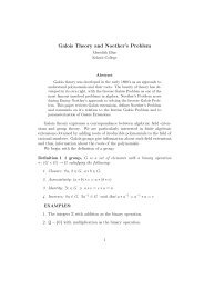
Definition<br />
The idea <strong>of</strong> a pursuit curve is that a point, which we<br />
will call the rabbit, follows a prescribed curve. The<br />
rabbit is followed by another point, which we will<br />
call the fox. Two conditions will be specified to<br />
determine a pursuit curve:<br />
1. The fox heads directly towards the rabbit.<br />
2. The fox’s speed is directly proportional to<br />
the rabbit’s.<br />
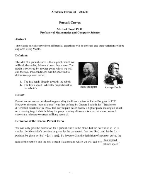
History<br />
Pierre Bouguer<br />
George Boole<br />
<strong>Pursuit</strong> curves were considered in general by the French scientist Pierre Bouguer in 1732.<br />
However, the term “pursuit curve” was first defined by George Boole in his “Treatise on<br />
differential equations” in 1859. The curved path described by a fighter plane making an attack<br />
on a moving target while holding the proper aiming allowance is a pursuit curve, so such<br />
curves are relevant to current military research.<br />
Derivation <strong>of</strong> the General <strong>Pursuit</strong> Curve<br />
n<br />
We will only give the derivation for a pursuit curve in the plane, but the derivation in R is<br />
similar. Let the rabbit’s position be given by the parametric function R (t)<br />
, and let the fox’s<br />
position be given by F ( t ) = x(<br />
t),<br />
y(<br />
t)<br />
. By Property 2 in the definition <strong>of</strong> a pursuit curve, the<br />
fox's speed<br />
ratio <strong>of</strong> the rabbit’s and the fox’s speed is a constant, which we will call k =<br />
.<br />
rabbit's speed<br />
4
Academic Forum 24 2006-07<br />
Property 1 in the definition <strong>of</strong> a pursuit curve, and the accompanying<br />
diagram make it clear that the unit tangent vector to the fox’s curve is<br />
F′<br />
R − F<br />
= . By the definition <strong>of</strong> k, F ′ = k R′<br />
. Substitute this into the<br />
F′<br />
R − F<br />
previous equation to obtain the vector differential equation describing the<br />
R − F<br />
general pursuit curve: F′ = k R′<br />
R − F<br />
This system <strong>of</strong> nonlinear differential equations must be solved by numerical methods except for<br />
special cases. It is left to the reader as an exercise to use the chain rule to see that the<br />
parameterization <strong>of</strong> the rabbit’s path will not affect the shape <strong>of</strong> the fox’s path. Thus, we may<br />
parameterize the rabbit’s path using any convenient function, and it does not matter that the<br />
rabbit’s speed may not be constant.<br />
Special Case <strong>of</strong> Pursuing a Straight Line Target<br />
Without loss <strong>of</strong> generality, we may assume that the rabbit runs up the y-axis, and parameterize<br />
the its path by R ( t ) = 0,<br />
rt . Let the fox’s initial position be given by F ( 0) = c,<br />
0 , where c is a<br />
positive constant. The vector differential equation for the fox simplifies to the system<br />
⎧ krx<br />
⎪x′<br />
= −<br />
2<br />
2<br />
⎪ x + ( rt − y)<br />
⎨<br />
.<br />
⎪ kr(<br />
rt − y)<br />
y′<br />
=<br />
⎪<br />
2<br />
2<br />
⎩ x + ( rt − y)<br />
dy y′<br />
y − rt<br />
Obtain = = from the chain rule and this system. Differentiate both sides with<br />
dx x′<br />
x<br />
2<br />
d y dt<br />
respect to x and simplify to obtain x = −r<br />
. Use the chain rule and Calculus to obtain<br />
2<br />
dx dx<br />
dt<br />
dx<br />
=<br />
dt<br />
ds<br />
⋅<br />
ds<br />
dx<br />
dt<br />
Eliminate dx<br />
1<br />
= −<br />
kr<br />
⎛ dy ⎞<br />
1+<br />
⎜ ⎟<br />
⎝ dx ⎠<br />
2<br />
ds<br />
. Note that is negative because s increases as x decreases.<br />
dx<br />
from the last two equations to get the second order, nonlinear differential<br />
2<br />
2<br />
d y ⎛ dy ⎞<br />
dy<br />
equation kx = 1+<br />
2<br />
⎜ ⎟ . We may reduce the order by substituting v = where v = 0<br />
dx ⎝ dx ⎠ dx<br />
dv<br />
2<br />
and x = c to get k = 1+<br />
v . This separable differential equation is solved to obtain<br />
dx<br />
1/ k 1/ k<br />
dy 1 ⎡⎛<br />
x ⎞ ⎛ c ⎞ ⎤<br />
= ⎢⎜<br />
⎟ − ⎜ ⎟ ⎥ . The last equation is integrated again to get the fox’s path, albeit in<br />
dx 2 ⎢⎣<br />
⎝ c ⎠ ⎝ x ⎠ ⎥⎦<br />
nonparametric form:<br />
5<br />
F<br />
(0,0)<br />
R-F<br />
R
Academic Forum 24 2006-07<br />
⎧1<br />
⎡<br />
⎪ ⎢<br />
⎪2<br />
⎣c<br />
y = ⎨<br />
⎪1<br />
⎡ x<br />
⎪ ⎢<br />
⎩2<br />
⎣<br />
1/ k<br />
2<br />
1+<br />
1/ k<br />
1/ k 1−1/<br />
x c x<br />
−<br />
(1 + 1/ k)<br />
1−1/<br />
k<br />
− c<br />
2c<br />
2<br />
x ⎤<br />
− c ln ⎥ if k = 1<br />
c ⎦<br />
k<br />
⎤<br />
⎥ +<br />
⎦<br />
ck<br />
if<br />
2<br />
k −1<br />
k ≠ 1<br />
If k > 1, which corresponds to the rabbit running faster than the fox, the fox will catch the<br />
rabbit when x = 0 , which implies<br />
will be t =<br />
y<br />
r<br />
ck<br />
y = . The time it will take the fox to catch the rabbit<br />
k 2 −1<br />
, and the total distance that the fox runs will be<br />
2<br />
ck<br />
krt = . k<br />
2<br />
−1<br />
It is more interesting to consider the second case k = 1, which corresponds to the rabbit running<br />
at the same speed as the fox. In this case,<br />
2<br />
c ⎡1<br />
x<br />
obtain t = ⎢ −<br />
2r<br />
⎣2<br />
2c<br />
2<br />
dt<br />
dx<br />
1<br />
= −<br />
r<br />
1 ⎛ x<br />
1+<br />
⎜<br />
4 ⎝ c<br />
−<br />
2<br />
c ⎞<br />
⎟<br />
x ⎠<br />
, which is integrated to<br />
x ⎤<br />
− ln ⎥ . Thus, the difference between the y coordinates <strong>of</strong> the rabbit and<br />
c ⎦<br />
2 2<br />
2<br />
1 ⎡ x − c x ⎤ c ⎡ ⎛ x ⎞ ⎤<br />
fox is yrabbit<br />
− y<br />
fox<br />
= rt − ⎢ − c ln ⎥ = ⎢1<br />
− ⎜ ⎟ ⎥ . Therefore,<br />
2 ⎣ 2c<br />
c ⎦ 2 ⎢⎣<br />
⎝ c ⎠ ⎥⎦<br />
c<br />
lim R ( t)<br />
− F(<br />
t)<br />
= lim( yrabbit<br />
− y<br />
fox<br />
) = . In other words, the fox will only cut the distance<br />
t→∞<br />
x↓0<br />
2<br />
between the rabbit and himself by 2 in the long run. The poor fox will never catch the rabbit!<br />
The computer algebra s<strong>of</strong>tware Maple dsolve and<br />
deplot commands were used to create the following<br />
curves. Originally, all the pursuit curves that I created<br />
in Maple were animated in a PowerPoint<br />
demonstration. Interestingly, the surface obtained by<br />
revolving the fox’s curve about the y-axis is a model<br />
for Lobachevsky’s version <strong>of</strong> non-Euclidean<br />
geometry (1829).<br />
Nikolai<br />
Ivanovich<br />
Lobachevsky<br />
(1792-1856)<br />
Here are typical Maple commands that were used to create the above and subsequent pursuit<br />
curves:<br />
> with(plots):<br />
> with(LinearAlgebra):<br />
6
Academic Forum 24 2006-07<br />
Warning, the name changecoords has been redefined<br />
> k:=.8:<br />
> R:=:<br />
> F:=:<br />
> FP:=map(z->diff(z,t),F):<br />
> RS:=k*(R-F)*Norm(map(z->diff(z,t),R),2,conjugate=false)/Norm(R-F,2,conjugate=false);<br />
> tmax:=10:<br />
> fmax:=200:<br />
> p:= dsolve({FP[1]=RS[1],FP[2]=RS[2],x(0)=0,y(0)=0}, {x(t),y(t)},type=numeric):<br />
> fp:=odeplot(p,[[x(t),y(t)],[R[1],R[2]]],0..tmax,frames=fmax):<br />
> rp:=animate(pointplot,[[[R[1],R[2]]], symbol=circle, symbolsize=10],t=0..tmax, frames=fmax):<br />
> display(fp,rp);<br />
Special Case <strong>of</strong> a the Rabbit Moving in a Circle<br />
Trajectories<br />
If k = 1, note that the distance between<br />
the fox and the rabbit is approaching<br />
zero. If k > 1, then the fox will catch<br />
the rabbit in finite time.<br />
Distance between the<br />
Animals vs. Time<br />
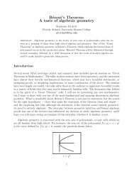
If k < 1, then the fox is attracted to a circle with strictly smaller<br />
diameter. In the picture shown here, the fox is traveling at 70% the<br />
rabbit’s speed.<br />
To derive the radius <strong>of</strong> this circle, assume that 0 < k ≤ 1 and<br />
parameterize the rabbit’s path by R ( t)<br />
= cost,<br />
sin t . Then the fox’s<br />
path can be parameterized by F ( t)<br />
= k cos( t − b),sin(<br />
t − b)<br />
where b is<br />
the angle that the fox lags behind. It is clear from the right triangle in<br />
the accompanying diagram that b = cos −1 k and<br />
lim R − F =<br />
2<br />
1−<br />
k .<br />
t→∞<br />
R<br />
b<br />
F<br />
7
Academic Forum 24 2006-07<br />
If k < 0 , then the fox will run away from the rabbit. If the fox’s<br />
initial position is the origin, then it will follow the negative y-axis for<br />
many values <strong>of</strong> negative k. If the fox’s initial position is ( 0,0.2)<br />
, then<br />
it will exit in the second quadrant approaching a straight line.<br />
The picture shown here is for a rabbit traveling along a triangle<br />
where k = 0.5 . Although the rabbit instantly changes direction<br />
at the corners, the fox’s path is a smooth triangular shape.<br />
The picture here shows a rabbit<br />
following a sine wave<br />
where k = 0.9 . If 0 .6 < k < 1,<br />
then the fox’s path appears to<br />
follow a damped sine wave. If<br />
k < 0.6 , then the fox lags<br />
further and further behind the<br />
rabbit and its path approaches<br />
the x-axis.<br />
8
Academic Forum 24 2006-07<br />
The path <strong>of</strong> a rabbit running on a cycloid<br />
R ( t)<br />
= t − sin t,1<br />
− cos t is similar to the above case.<br />
The picture shown here is for a rabbit running along a threeleaved<br />
rose r = cos( 3θ<br />
) . The fox appears to be approaching a<br />
similar, but rotated slightly counter-clockwise curve.<br />
I tried to have the rabbit randomly walk in the plane, but Maple’s<br />
dsolve command gave an error when I tried to pass it the rabbit’s<br />
path function.<br />
Here are some ideas for further investigation:<br />
• Find the equations for the attractors for sinusoidal and triangular paths for the rabbit<br />
• Investigate this problem in three or higher dimensions.<br />
• What if one fox is pursuing two rabbits?<br />
• Incorporate delayed reaction time or anticipation into the model. If δ is the delay time,<br />
R(<br />
t −δ<br />
) − F(<br />
t)<br />
then the differential equation becomes F′<br />
( t)<br />
= k R′<br />
( t −δ )<br />
.<br />
R(<br />
t −δ<br />
) − F(<br />
t)<br />
• Allow for speed <strong>of</strong> transmission. For example, if the fox uses sonar to detect the rabbit,<br />
then incorporate the speed <strong>of</strong> sound.<br />
• Determine exit path dependence on fox’s initial position for retreat curve when the<br />
rabbit is traveling in a circle.<br />
• Find critical k where fox cannot keep up with a sine wave.<br />
9
Academic Forum 24 2006-07<br />
Sources<br />
• “Differential Equation with Application and Historical Notes” by George F. Simmons<br />
(c)1972 by McGraw Hill<br />
• http://www.answers.com/topic/curve-<strong>of</strong>-pursuit<br />
• “In <strong>Pursuit</strong>” by Peter M. Gent, April 17, 1999<br />
http://online.redwoods.cc.ca.us/instruct/darnold/StaffDev/assignments/pursuit.pdf<br />
• “<strong>Pursuit</strong> <strong>Curves</strong> and Matlab” by Peter M. Gent<br />
http://online.redwoods.cc.ca.us/instruct/darnold/deproj/Sp98/PeterG/<br />
• “<strong>Pursuit</strong> Curve” http://mathworld.wolfram.com/<strong>Pursuit</strong>Curve.html<br />
• “The MacTutor History <strong>of</strong> Mathematics Archive” http://www-groups.dcs.stand.ac.uk/~history/<br />
Biography<br />
Michael Lloyd received his B.S in Chemical Engineering in 1984 and accepted a position at<br />
Henderson State University in 1993 after earning his Ph.D. in Mathematics from Kansas State<br />
University. He has presented papers at meetings <strong>of</strong> the Academy <strong>of</strong> Economics and Finance,<br />
the <strong>America</strong>n <strong>Mathematical</strong> Society, the Arkansas Conference on Teaching, the <strong>Mathematical</strong><br />
<strong>Association</strong> <strong>of</strong> <strong>America</strong>, and the Southwest Arkansas Council <strong>of</strong> Teachers <strong>of</strong> Mathematics. He<br />
has also been an AP statistics consultant since 2001 and a member <strong>of</strong> the <strong>America</strong>n Statistical<br />
<strong>Association</strong>.<br />
10