Theoretische Physik 2: Elektrodynamik Tutorial 2 - Institut für ...

WiSe 2012 23.10.2012
Prof. Dr. A.-S. Smith
Dipl.-Phys. Ellen Fischermeier
Dipl.-Phys. Matthias Saba
am Lehrstuhl für Theoretische Physik I
Department für Physik
Friedrich-Alexander-Universität
Erlangen-Nürnberg
Theoretische Physik 2: Elektrodynamik
(Prof. A.-S. Smith)
Tutorial 2
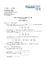
Tutorial 2.1 Differential operators in cylindrical coordinates
In cartesian coordinates the nabla operator is defined as follows:
∂
⃗∇ = ⃗e x
∂x + ⃗e ∂
y
∂y + ⃗e ∂
z
∂z
Cylindrical coordinates (ρ, φ, z) are defined as follows:
x = ρ cos φ, y = ρ sin φ, z = z
a) Transform the nabla operator into cylindrical coordinates. Proceed with the following steps:
• Use the chain rule to write the partial derivatives ∂/∂x, ∂/∂y and ∂/∂z in terms of ∂/∂ρ,
∂/∂φ, ∂/∂z
• Write ⃗e x , ⃗e y and ⃗e z in terms of ⃗e ρ , ⃗e φ , ⃗e z
Result: ∇ ⃗ ∂
= ⃗e ρ ∂ρ + ⃗e φ 1 ∂
ρ ∂φ + ⃗e z ∂ ∂z
b) Calculate for a vector field A ⃗ the expression ∇ ⃗ · ⃗A
Result: ∇ ⃗ · ⃗A = 1 ∂
ρ ∂ρ (ρA ρ) + 1 ∂
ρ ∂φ (A φ) + ∂ ∂z (A z)
Tutorial 2.2
Newton’s theorem
a) Prove the electrostatic analog of Newton’s theorem:
For a spherically symmetric charge (or mass, in the case of gravity) distribution ρ(r),
the radial component of the electric field, E r = E ⃗ · ⃗r/r, is given by
E r = Q(r)
r 2 with Q(r) = 4π
∫ r
0
ρ(R)R 2 dR ,
i. e. the same as if the charge in the sphere of radius R is located at the center of the
sphere.

Calculate also the associated electrostatic potential.
Note that the Poisson equation in spherical coordinates reads
−4πρ = ∇ 2 ϕ = 1 (
∂
r 2 r 2 ∂ϕ )
1 ∂
+
∂r ∂r r 2 sin ϑ ∂ϑ
(
sin ϑ ∂ϕ
∂ϑ
)
+
1 ∂ 2 ϕ
r 2 sin 2 ϑ ∂φ 2 .
b) As an application of Newton’s theorem, consider a charge-free spherical cavity concentric with
the center of a spherically symmetric charge distribution. What is the electric force on a test
charge inside this hole?
Tutorial 2.3
Stable rest position in an electrostatic field
Consider a time-independent electric field ⃗ E(⃗x) with the property that for a point particle with charge
q > 0 the position ⃗x = 0 is a stable rest position with a linear reset force. That is, for the force ⃗ F = q ⃗ E,
the following properties hold:
• ⃗ F is zero at ⃗x = 0.
• In the vicinity of ⃗x = 0 ⃗ F forces the particle back to ⃗x = 0. ⃗ F (⃗x) can be regarded as a linear
function of ⃗x for small displacements.
The magnetic field is zero.
Show that the charge density ρ(⃗x), that creates the field E, ⃗ cannot have a zero at ⃗x = 0.
sign does ρ(0) have?
What
Hint: The relation ⃗ ∇ × ⃗ E = 0 follows from the induction law. Use that fact to show that A ij :=
− ∂
∂x j
E i (⃗x = 0) is a symmetric matrix. Now choose the coordinate axes parallel to the direction of the
principal axes of A ij and calculate in this coordinate system the charge density ρ(⃗x).
Tutorial 2.4
Penning trap
Consider the motion of a particle that has a charge q and mass m in a constant uniform magnetic field
⃗B = Bê z and an electric quadrupole potential (U 0 > 0)
ϕ(⃗x) = − U 0
2r0
2 (x 2 + y 2 − 2z 2 ) , ⃗x = (x, y, z) .
a) Show that the non-relativistic equation of motion for the particle in the x–y plane for the case
U 0 = 0 leads to oscillatory motion. Determine the cyclotron frequency ω c characterizing the
oscillation. It is favorable to introduce a complex variable ξ := x + iy.
b) Determine the electric field ⃗ E(⃗x) = − ⃗ ∇ϕ(⃗x) and verify that ⃗ E is solenoidal, i.e., ⃗ ∇ · ⃗E(⃗x) = 0.
c) Show that the magnetic field does not couple to the motion along the z-direction, and determine
the characteristic frequency ω z for the corresponding harmonic oscillations in the quadrupole
field.
d) Solve the complete equations of motion in the x–y plane and show that the general solution
is a superposition of two oscillatory motions with a perturbed cyclotron frequency ω ′ c and the
magnetron frequency ω M . Provide conditions such that the orbits are stable. Discuss the case
ω z ≪ ω c in particular.

Tutorial 2.5
Cylindrical capacitor
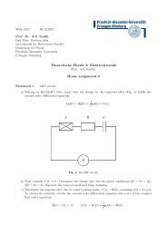
a) Using Gauß’ law, calculate the capacitance of two concentric conducting cylinders of length L,
when L is large compared to their radii a, b (a < b). Apply the result to calculate the inner
diameter of the outer conductor in an air-filled coaxial cable whose center is a cylindrical wire
of diameter 1 mm and whose capacitance is 0.5 × 10 −6 µF cm −1 .
b) For the cylindrical capacitor from part a) calculate the total electrostatic energy and express
it alternatively in terms of the equal and opposite charges Q and −Q placed on the capacitor
plates and the potential difference between the plates.
Sketch the energy density of the capacitor’s electrostatic field as a function of the appropriate
linear coordinate.
c) Two long, parallel, cylindrical conductors of radii a 1 and a 2 are separated by a distance d, which
is large compared with either radius. Show that the capacitance per unit of length is given
approximately by
[ ( )]
C d −1
L ≃ 4 ln ,
a
where a is the geometrical mean of the two radii.
(i) What gauge wire (state the radius in millimetres) would be necessary to make a two-wire
transmission line with a capacitance of 0.1 pF cm −1 , if the separation of the wires is 0.5
cm, 1.5 cm, and 5.0 cm?
d) Calculate the attractive force per unit length between the two conductors in a parallel cylindrical
capacitor for:
(i) fixed charges on each conductor,
(ii) a fixed potential difference between the conductors.
Due date: Thursday, 25.10.12, at 13:00

WiSe 2012 23.10.2012
Prof. Dr. A.-S. Smith
Dipl.-Phys. Ellen Fischermeier
Dipl.-Phys. Matthias Saba
am Lehrstuhl für Theoretische Physik I
Department für Physik
Friedrich-Alexander-Universität
Erlangen-Nürnberg
Theoretische Physik 2: Elektrodynamik
(Prof. A.-S. Smith)
Solutions to Tutorial 2
Solution of Tutorial 2.1
a)
Use the chain rule:
Differential operators in cylindrical coordinates
x = ρ cos φ, y = ρ sin φ, z = z
∂f
∂ρ = ∂x ∂f
∂ρ ∂x + ∂y ∂f
∂ρ ∂y + ∂z ∂f
∂ρ ∂z
= cos φ∂f + sin φ∂f
∂x ∂y
Analogously:
So with
we get
∂f
∂φ
∂f
∂z
= −ρ sin φ∂f + ρ cos φ∂f
∂x ∂y
= ∂f
∂z
∂
∂ρ = ∂ ρ = cos φ ∂ x + sin φ ∂ y
1 ∂
ρ ∂φ = 1 ρ ∂ φ = − sin φ ∂ x + cos φ ∂ y
∂ x = cos φ ∂ ρ − 1 ρ sin φ ∂ φ
∂ y = sin φ ∂ ρ + 1 ρ cos φ ∂ φ
∂ z = ∂ z
Now the unit vectors:
⃗e ρ =
∂⃗x
−1 ∂⃗x
∣ ∂ρ ∣
∂ρ , . . . 1

With
follows
⃗x = x⃗e x + y⃗e y + z⃗e z = ρ cos φ ⃗e x + ρ sin φ ⃗e y + z⃗e z
⃗e ρ = cos φ ⃗e x + sin φ ⃗e y
⃗e φ = − sin φ ⃗e x + cos φ ⃗e y
⃗e z = ⃗e z
All together:
b) It holds:
=⇒ ⃗e x = cos φ ⃗e ρ − sin φ ⃗e φ , ⃗e y = sin φ ⃗e ρ + cos φ ⃗e φ
⃗∇ = ⃗e x ∂ x + ⃗e y ∂ y + ⃗e z ∂ z = . . . = ⃗e ρ ∂ ρ + ⃗e φ
1
ρ ∂ φ + ⃗e z ∂ z
• ⃗e x ⊥ ⃗e y ⊥ ⃗e z and ⃗e ρ ⊥ ⃗e φ ⊥ ⃗e z due to ⃗e i · ⃗e j = δ ij
⎛ ⎞
⎛ ⎞
− sin φ
− cos φ
• ∂ φ ⃗e ρ = ⎝ cos φ
0
⎠ = ⃗e φ ∂ φ ⃗e φ = ⎝ − sin φ
0
⎠ = −⃗e ρ ∂ φ ⃗e z = 0
• ∂ ρ ⃗e φ = ∂ ρ ⃗e ρ = ∂ ρ ⃗e z = ∂ z ⃗e φ = ∂ z ⃗e ρ = ∂ z ⃗e z = 0
and therefore ⃗ ∇ · ⃗A in cylindrical coordinates is
⃗∇ · ⃗A = (⃗e ρ ∂ ρ + ⃗e φ
1
ρ ∂ φ + ⃗e z ∂ z ) · (A ρ ⃗e ρ + A φ ⃗e φ + A z ⃗e z ) =
= ∂ ρ A ρ + 1 ρ A ρ + 1 ρ ∂ φA φ + ∂ z A z = 1 ρ ∂ρ (ρA ρ) + 1 ρ ∂φ (A φ) + ∂ ∂z (A z)
∂
∂
Solution of Tutorial 2.2
Newton’s theorem
a) Poisson’s equation for the charge density simplifies since the electrostatic potential depends
solely on the radial distance,
4πρ(r) = −∇ 2 ϕ(r) = − 1 (
d
r 2 r 2 dϕ )
= 1 d
dr dr r 2 dr (r2 E r ).
where E r = −⃗r/r · ⃗∇φ denotes the radial component of the electric field. Integrating once
4π
∫ r
0
ρ(R)R 2 dR = r 2 E r (r)
or
E r (r) = Q(r)
∫ r
r 2 with Q(r) = 4π ρ(R)R 2 dR.
0
This result allows for a neat interpretation. The electric field corresponding to a spherically
symmetric charge distribution at radial distance r is identical to one where the charge contained
in the sphere of that radius is concentrated in the origin.
The potential is obtained by integrating once more,
ϕ(r) =
∫ ∞
r
Q(R)
R 2 dR.
[The point of the reference potential is at infinity, ϕ(∞) = 0.]
b) The force on the test charge is proportional to the electric field. Newton’s theorem implies a
vanishing force at the inside, since the charge distribution equals zero there.
2

Solution of Tutorial 2.3
Stable rest position in an electrostatic field
⃗E(⃗x) is a linear function of ⃗x in the vicinity of ⃗x = 0.
Because of ⃗ E(0) = 0 ⇒ E 0j = 0.
⇒ E j (⃗x) = E 0j − A jl x l + O(r 2 ) (1)
⇒ (curl ⃗ E) l = ε lmn ∂ m E n = −ε lmn ∂ m A nj x j + O(r) =
= −ε lmn A nj δ mj + O(r) = −ε lmn A nm + O(r) = 0
⇒ ε lmn A nm = 0 ⇒ A nm = A mn (symmetric matrix)
For example for l = 1 : ε 1mn A nm = ε 123 A 32 + ε 132 A 23 = A 32 − A 23 = 0 ⇒ A 32 = A 23 (Analogously
for the other components).
Because A jl is symmetric and real (because E ⃗ is real) a principal axis transformation can be done
so that A jl is diagonal in this new coordinate system, that means A jl = 0 for j ≠ l. The diagonal
elements must be > 0 because otherwise the field in (1) would not show in the direction of the origin
for a positive test charge and the resulting force would not be a linear reset force.
⇒ ρ(⃗x) = ε 0 div ⃗ E = ε 0 ∂ l E l = −ε 0 A lj ∂ l x j
}{{}
=δ lj
+O(r) = −ε 0 A ll + O(r)
⇒ ρ(0) = −ε 0 A ll < 0
At the origin there must be a nonzero, negative charge.
⇒ It is not possible to place charges out of a charge-free cavity, so that there is a potential within the
cavity that produces a stable rest position with a linear reset force.
Solution of Tutorial 2.4
Penning trap
For a particle in an electromagnetic field, Newton’s equation balances inertial forces and the Lorentz
force with contributions from the electric and the magnetic field,
}{{} m¨⃗x = −q∇ϕ
} {{ ⃗ }
inertial electric
+ q c ˙⃗x × B ⃗ .
} {{ }
magnetic
In our case, B ⃗ = B⃗e z and ϕ(⃗x) = −(U 0 /2R0 2)(x2 + y 2 − 2z 2 ).
a) Without quadrupole field, U 0 = 0. The equations of motion in components are
mẍ = q c ẏB , mÿ = −q c ẋB .
Complexify, ξ = x + iy. Then with the cyclotron frequency ω c = qB/mc ,
¨ξ = −iω c ˙ξ , with the solution ξ(t) = ξ0 + Ae iα e −iωct
with a real amplitude A and phase α. Decomposing into cartesian components again, yields
x(t) = x 0 + A cos(ω c t − α) , y(t) = y 0 − A sin(ω c t − α) ,
i.e., circular orbits spinning counter-clockwise. The centers (x 0 , y 0 ) are arbitrary.
3

) Taking the gradient of the potential yields the electric field,
⎛ ⎞
⃗E(⃗x) = −∇ϕ(⃗x) ⃗ = U x
0
⎝
r0
2 y ⎠ ,
−2z
the divergence of which vanishes,
−∇ 2 ϕ = ∇ ⃗ · ⃗E = U 0
r0
2 (1 + 1 − 2) = 0 .
Thus, the Laplace equation tells us that it is solenoidal, i.e., there are no charges.
c) The motion in the z-direction is governed by
¨z = qE z
m = −2qU 0
z ≡ −ωzz 2 ;
mr 2 0
the magnetic field does not couple to the parallel motion. The solution is again a harmonic
oscillation around the center of the trap,
z(t) = a z cos(ω z t − ψ) .
d) Now, we consider both the magnetic and the quadrupol field,
In terms of the complex variable,
mẍ = q c ẏB + qU 0
r0
2 x ,
mÿ = − q c ẋB + qU 0
r0
2 y .
¨ξ = −iω c ˙ξ +
ω 2 z
2 ξ .
This second-order, linear differential equation with constant coefficients is solved using the
Ansatz ξ(t) ∝ e −iωt . The characteristic frequency is then determined by
ω 2 − ω c ω + ω2 z
2 = 0 .
The two solutions are a reduced cyclotron frequency,
and the so-called magnetron frequency,
ω ′ c = ω c
2 + √
ω 2 c
4 − ω2 z
2 ≈ ω c − ω2 z
2ω c
+ O(ω 4 z) ,
ω M = ω c
2 − √
ω 2 c
4 − ω2 z
2 ≈ ω2 z
2ω c
+ O(ω 4 z) .
Stability requires both frequencies to be real, i.e., 2ω 2 z < ω 2 c , or in terms of the magnetic field
The general solution then reads
or in cartesian components,
B 2 > 2m2 c 2 ω 2 z
q 2
= 4mc2
qr0
2 U 0 .
ξ(t) = Ae iα e −iω′ c t + Be iβ e −iω M t ,
x(t) = A cos(ω ′ ct − α) + B cos(ω M t − β) ,
y(t) = −A sin(ω ′ ct − α) − B sin(ω M t − β) .
4

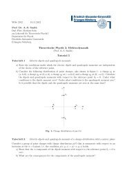
In general, Penning trap parameters are chosen such that
the radius of magnetron motion exceeds that of the cyclotron
motion by a factor of the order 100 and ω M ≪ ω z ≪
ω c . The orbits consist then of a rapid cyclotron motion of
small radius whereas the centers slowly follow another circular
trajectory. The Penning trap was co-invented by the
German-born American physicist Hans Georg Dehmelt, who
received the Nobel prize in 1989 together with Wolfgang
Paul (Paul trap).
Linguistic note: pen means ’Laufstall’, ’Einzäunung’.
Ω c ⩵20Ω M
Solution of Tutorial 2.5
Cylindrical capacitor
Fig. 1: Orbits in a Penning trap for commensurate
frequencies
a) To find the capacitance of the cylindrical capacitor that is formed by the two cylinders, we give
them equal and opposite charge and find the ratio of this charge to the potential difference
between them. So let the inner and the outer cylinders have a uniformly-spread total charge
of +Q and −Q respectively (Fig. 1). Since the length L of the cylinders is much larger than
their radii, the electric field between the cylinders can be approximated by that for the case
of infinitely long cylinders, and we can ignore the end effects. Now imagine a cylinder (here
denoted by S(ρ)) between the two given cylinders, i.e., coaxial with the two given cylinders, and
with a radius ρ satisfying a < ρ < b. Applying Gauß’ law for this cylinder:
∮
⃗E · dS ⃗ = 4πQ
∮
S(ρ)
⃗E · d ⃗ S =
∫
sheet
S(ρ)
E(ρ)⃗e ρ · ⃗e ρ dS = E(ρ)
E(ρ) 2πρL = 4πQ
E = 2λ ρ ; ⃗ E = 2λ ρ ⃗e ρ .
∫
sheet
dS = E(ρ) 2πρL
where "sheet" denotes the curved part of S(ρ), and λ is the line charge density. The potential
difference between the two cylinders is then
∫ a
∫ b
( )
Φ(a) − Φ(b) = − ⃗E · d ⃗ ⃗e ρ
b
l = 2λ
b
a ρ · ⃗e ρ dr = 2λ ln ,
a
Electric capacitance of the cylindrical capacitor is therefore
C = Q U =
L
2 ln(b/a) .
From this, it follows that the radius of the outer cylinder is
( ) L
b = a exp .
2C
Therefore, for the given values,
In CGS system of units
2a = 1 mm
C
L = 0.5 × 10−6 µF cm −1 .
Fig. 2: Cylindrical capacitor.
5

1 F = 9 × 10 11 cm.
Therefore C L = (0.5 × 10−6 ) (9 × 10 5 ) = 4.5 × 10 −1 , which gives 2b = 2 × 0.5 exp ( 10
9
b) The potential energy of a system of n charged conductors is
W = 1 2
n∑
Q i V i .
i=1
In our case, the number of conductors is n = 2. Hence,
W = 1 2 QV 1 + 1 2 (−Q)V 2 = 1 2 Q(V 1 − V 2 ) = 1 2 QU ,
where U is the potential difference. By definition
Therefore, the electrostatic energy is
C = Q U .
W (Q) = 1 Q 2
2 C
W (U) = 1 2 CU 2 .
We have already shown that the capacitance of the cylindrical capacitor equals
C =
so its energy in terms of the charge Q is simply
and in terms of the potential difference U is
L
2 ln(b/a) ,
W (Q) = ln(b/a)
L Q2 ,
W (U) =
The relation for the energy density reads
ω = 1
∣E
8π
⃗ ∣ 2 .
The electric field in the cylindrical capacitor
equals
⃗E = 2λ ρ ⃗e ρ , a < ρ < b ,
L
4 ln(b/a) U 2 .
)
= 3.04 mm
where ⃗e ρ is the unit vector in the direction
of the cylindrical coordinate ρ. The energy
density is then
ω = 1 λ 2
2π ρ 2 , a < ρ < b .
Fig. 3: Energy density in the cylinder capacitor as a
function of the distance from the axis of the
capacitor. We set b → ∞.
6

c) As the separation of the cylinders d is much larger than their radii a 1 and a 2 (Fig. 3), if they
are charged, then we can assume that the electric field of each distribution will not affect the
other one much, and so the charge distributions can be assumed to be uniform. (Note: When
the separation is comparable to their radii, this assumption is not valid.) Hence, let this uniform
charge per unit length be +λ on the cylinder with radius a 1 and −λ on the one with radius a 2 .
From part a), the potential of a cylinder with a uniform line charge distribution λ is
( ) A
Φ(ρ) = 2λ ln ,
ρ
(with the axis of the cylinder aligned with the z-axis of coordinate system and A an arbitrary
radial distance for which Φ(A) = 0).
(
) (
)
A
A
Φ = Φ 1 + Φ 2 = 2λ ln √ − 2λ ln √
x 2 + (y − d/2) 2 x 2 + (y + d/2) 2
( x 2 + (y + d/2) 2 )
= λ ln
x 2 + (y − d/2) 2 .
The surfaces of the cylinders are equipotential
because the cylinders are conductors. For the
cylinder 1 we have
x = a 1 cos ϕ 1
y = d 2 + a 1 sin ϕ 1 .
Therefore the potential Φ(1) (of cylinder 1) is
( a
2
Φ(1) = λ ln 1 cos 2 ϕ 1 + (a 1 sin ϕ 1 + d) 2 )
a 2 1 cos ϕ2 1 + a2 1 sin ϕ2 1
( a
2
= λ ln 1 + 2da 1 sin ϕ 1 + d 2 )
a 2 1
(
= λ ln 1 + 2a (
1
d sin ϕ a1
) ) ( )
2 d
1 + + 2λ ln .
d
a 1
Because d ≫ a 1 we can approximate the first logarithmic term by
(
ln 1 + 2a (
1
d sin ϕ a1
) ) 2
1 + ≃ ln 1 = 0 .
d
Fig. 4: Separated cylindrical conductors.
With this approximation the potential Φ(1) is
( ) d
Φ(1) ≃ 2λ ln
a 1
.
Similarly, we can determine the potential over the surface of cylinder 2
x = a 2 cos ϕ 2
y = − d 2 + a 2 sin ϕ 2
(
a 2 ) ( )
2
d
Φ(2) = λ ln
a 2 2 − 2da 2 sin ϕ 2 + d 2 ≃ −2λ ln
a 2
.
7

Hence the potential difference is
U = Φ(1) − Φ(2) = 2λ ln
where a is the geometric mean of the radii
a = √ a 1 a 2 .
( ) ( d
2
d
= 4λ ln ,
a 1 a 2 a)
Therefore the capacitance per unit length is
C
L = λ [ ( )] d −1
U = 4 ln .
a
(i) We are given
C
L = 0.1 pF cm−1 = 9 × 10 −2
and we can easily express a in terms of the capacitance per unit length and the wire
separation
(
a = d exp − L )
.
4C
Therefore, for separations d of 0.5 cm, 1.5 cm, and 5.0 cm, we get a wire radius of 0.31 mm,
0.93 mm, and 3.11 mm, respectively.
Note that for the given capacitance, the condition d ≫ a 1 , a 2 is satisfied, and hence we are
allowed the use of the approximate formula that we have derived.
d) (i) From part b), the total electrostatic energy is W (Q) = 1 2 C
. Therefore, the electrostatic
energy per unit of length (for two parallel, very long conductors of radii a 1 and a 2 which
are separated by a distance d (d ≫ a 1 , a 2 )) is
( )
W Qλ (d) =
λ2
d
2(C/L) = 2λ2 ln ,
a
where λ is the charge per unit of length. The force per unit of length between conductors
reads
F = − ∂W Q λ
(d)
= − 2λ2
∂d d .
(ii) The electrostatic energy per unit of length expressed in terms of the potential difference
between the two cylinders is
U 2
W Uλ (d) = 1 8 ln (d/a) .
When we fix the potential difference between the cylinders and change their separation, the
source of voltage (battery) does some work, namely in increasing or decreasing the charge
on the cylinders of the capacitor. In this case, therefore, the change in the electrostatic
energy for the capacitor is not only due to the mechanical work involved (i.e., moving of
the capacitor’s plates) as it was case in (i), but also due to the source work which changes
the charge on the plates. That is,
Q 2
∆W U (d) = ∆W mech + ∆W source ,
where ∆W mech is the work done due to the moving of the plates, and ∆W source is the work
due to the charging or the discharging of the plates. The source work is
∆W source = ∆Q U
∆Q = U ∆C
∆W source = ∆C U 2 .
8

So, for the force per unit length, we can write
F = − ∂W mech λ
∂d
= − ∂W U λ
(d)
+ ∂W source λ
∂d ∂d
U 2
U 2
U 2
= 1 8 d ln 2 (d/a) − 1 4 d ln 2 (d/a) = −1 8 d ln 2 (d/a) ,
where for the capacitance per unit length of the cylindrical conductors we have used the
expression derived earlier
C
L = λ [ ( )] d −1
U = 4 ln .
a
On comparing this expression with the one obtained in part (i)
− 1 8
U 2
d ln 2 (d/a) = − 1
8d ln 2 (d/a) × (4λ ln(d/a))2 = − 2λ2
d ,
we see that the expressions are the same.
9