Software Reliability Analysis and Evaluation - LAAS CNRS
Software Reliability Analysis and Evaluation - LAAS CNRS
Software Reliability Analysis and Evaluation - LAAS CNRS

You also want an ePaper? Increase the reach of your titles
YUMPU automatically turns print PDFs into web optimized ePapers that Google loves.
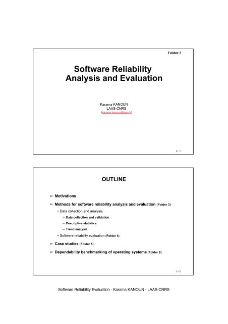
Folder 3<br />
<strong>Software</strong> <strong>Reliability</strong><br />
<strong>Analysis</strong> <strong>and</strong> <strong>Evaluation</strong><br />
Karama KANOUN<br />
<strong>LAAS</strong>-<strong>CNRS</strong><br />
(karama.kanoun@laas.fr)<br />
3 - 1<br />
OUTLINE<br />
☞ Motivations<br />
☞ Methods for software reliability analysis <strong>and</strong> evaluation (Folder 3)<br />
• Data collection <strong>and</strong> analysis<br />
☞ Data collection <strong>and</strong> validation<br />
☞ Descriptive statistics<br />
☞ Trend analysis<br />
• <strong>Software</strong> reliability evaluation (Folder 4)<br />
☞ Case studies (Folder 5)<br />
☞ Dependability benchmarking of operating systems (Folder 6)<br />
3 - 2<br />
<strong>Software</strong> <strong>Reliability</strong> <strong>Evaluation</strong> - Karama KANOUN - <strong>LAAS</strong>-<strong>CNRS</strong>
Why <strong>Software</strong> <strong>Reliability</strong>?<br />
☞ Increasing role of software in real life systems<br />
☞ System dependability is more <strong>and</strong> more synonymous of software<br />
reliability<br />
☞ Difficulties in mastering the software development process <strong>and</strong> in<br />
reducing design faults for complex systems<br />
☞ Increasing cost of system non-dependability<br />
☞ Real needs for improving software reliability to improve system<br />
dependability <strong>and</strong> reduce maintenance cost<br />
☞ Dependability requirements are part of system requirements (as<br />
important as functional requirements)<br />
☞ Quantification is essential<br />
3 - 3<br />
Objectives of software reliability analysis <strong>and</strong> evaluation<br />
☞ Manage <strong>and</strong> improve the reliability of software products<br />
☞ Check the efficiency of development activities<br />
☞ Estimate the “effort” needed to reach a high dependability level<br />
☞ Evaluate the software reliability at the end of validation activities <strong>and</strong> in<br />
operation<br />
☞ Estimate the maintenance effort to “correct” faults activated during<br />
development <strong>and</strong> residual faults in operation<br />
☞ Needs for experimental & analytical methods <strong>and</strong><br />
techniques to reach these objectives<br />
3 - 4<br />
<strong>Software</strong> <strong>Reliability</strong> <strong>Evaluation</strong> - Karama KANOUN - <strong>LAAS</strong>-<strong>CNRS</strong>
<strong>Software</strong> vs hardware reliability<br />
Hardware<br />
• Physical faults<br />
• Operational life<br />
• Stable reliability (constant failure rate)<br />
• White-box approach<br />
• Markov models<br />
• Database for components failures<br />
<strong>Software</strong><br />
• Only design faults<br />
• Development <strong>and</strong> operation<br />
• <strong>Reliability</strong> growth (↓ failure rate)<br />
• Usually black-box approach<br />
• Specific models<br />
• Based on data collection<br />
Failure Rate<br />
Hardware in operation<br />
<strong>Software</strong> in operation<br />
Time<br />
3 - 5<br />
Measures<br />
Static Measures<br />
of the product <strong>and</strong><br />
process<br />
(quality oriented)<br />
Usage profile<br />
(environment)<br />
Dynamic Measures<br />
characterizing occurrence of<br />
failures<br />
(reliability oriented)<br />
Number of faults<br />
Fault density<br />
Complexity measures<br />
…<br />
Failure intensity<br />
Failure rate<br />
MTTF<br />
<strong>Reliability</strong><br />
…<br />
3 - 6<br />
<strong>Software</strong> <strong>Reliability</strong> <strong>Evaluation</strong> - Karama KANOUN - <strong>LAAS</strong>-<strong>CNRS</strong>
☞ Supplier point of view<br />
• During development:<br />
☞development follow up<br />
(failure intensity, fault density)<br />
☞evaluation of software reliability before operation<br />
(MTTF, pre-operational failure rate)<br />
• During operation<br />
☞product reliability follow up<br />
(residual failure rate, MTTF)<br />
☞maintenance planning<br />
(cumulative number of failures)<br />
☞ Users / customers, operational life<br />
☞be confident in the reliability level of the product<br />
(residual failure rate, MTTF)<br />
3 - 7<br />
Percentage of faults <strong>and</strong> corresponding MTTF (published by IBM)<br />
Product<br />
MTTF (years)<br />
5000 1580 500 158 50 15.8 5 1.58<br />
⇐<br />
1<br />
2<br />
3<br />
4<br />
5<br />
6<br />
7<br />
8<br />
9<br />
34,2<br />
34,3<br />
33,7<br />
34,2<br />
34,2<br />
32,0<br />
34,0<br />
31,9<br />
31,2<br />
28,8<br />
28,0<br />
28,5<br />
28,5<br />
28,5<br />
28,2<br />
28,5<br />
27,1<br />
27,6<br />
17,8<br />
18,2<br />
18,0<br />
18,7<br />
18,4<br />
20,1<br />
18,5<br />
18,4<br />
20,4<br />
10,3<br />
9,7<br />
8,7<br />
11,9<br />
9,4<br />
11,5<br />
9,9<br />
11,1<br />
12,8<br />
5,0<br />
4,5<br />
6,5<br />
4,4<br />
4,4<br />
5,0<br />
4,5<br />
6,5<br />
5,6<br />
2,1<br />
3,2<br />
2,8<br />
2,0<br />
2,9<br />
2,1<br />
2,7<br />
2,7<br />
1,9<br />
1,2<br />
1,5<br />
1,4<br />
0,3<br />
1,4<br />
0,8<br />
1,4<br />
1,4<br />
0,5<br />
0,7<br />
0,7<br />
0,4<br />
0,1<br />
0,7<br />
0,3<br />
0,6<br />
1,1<br />
0,0<br />
⇐<br />
3 - 8<br />
<strong>Software</strong> <strong>Reliability</strong> <strong>Evaluation</strong> - Karama KANOUN - <strong>LAAS</strong>-<strong>CNRS</strong>
Overview of a global reliability analysis method<br />
Development<br />
Validation &<br />
Operation<br />
1<br />
Data related to<br />
previous projects,<br />
similar products<br />
data collection<br />
Objectives<br />
of the study<br />
Types<br />
of faults<br />
3<br />
Collected data<br />
2<br />
Data Validation<br />
Validated<br />
data<br />
Data set partition<br />
Consequences Phase Components<br />
of failures<br />
• • •<br />
4 Descriptive Analyses 5 Trend Analyses<br />
6 Model Application<br />
Descriptive Statistics<br />
<strong>Reliability</strong> Evolution<br />
<strong>Reliability</strong> Measures<br />
Feedback to the development process<br />
3 - 9<br />
☞ Some rules<br />
Setting up of a data collection process<br />
• Define clearly the objectives <strong>and</strong> the data to be collected<br />
• Motivate <strong>and</strong> imply people that will be involved<br />
• Simplify the collection process <strong>and</strong> reduce the number of data items to<br />
be collected<br />
☞ Support tools<br />
☞ Practical organization of people involved<br />
• Record <strong>and</strong> analyze data in real-time<br />
• Feedback<br />
☞ Origin of collected data<br />
• Internal: recorded during development <strong>and</strong> validation<br />
• External: by the customers<br />
3 - 10<br />
<strong>Software</strong> <strong>Reliability</strong> <strong>Evaluation</strong> - Karama KANOUN - <strong>LAAS</strong>-<strong>CNRS</strong>
Data to be collected<br />
☞ Background information<br />
• Product itself: software size, language, functions, current version, workload<br />
• Usage environment: verification <strong>and</strong> validation methods, tools, etc.<br />
☞ Data relative to failures <strong>and</strong> corrections<br />
• Date of occurrence, nature of failures, consequences<br />
• Type of faults, fault location<br />
☞ Usually, recorded through<br />
• Failure Reports (FR)<br />
• Correction Reports (CR)<br />
☞ Well defined headings, well structured, easy to fill in<br />
☞ Short tick-off questions<br />
☞ Manually or automatically<br />
3 - 11<br />
☞ Failure Report (FR)<br />
Required Information<br />
• Serial number (for identification)<br />
• Report editor<br />
• Product reference, version affected (or prototype)<br />
• Date <strong>and</strong> time of failure occurrence<br />
Desirable Information<br />
• Failure occurrence condition<br />
• Failure criticality or consequences<br />
• Affected function or task<br />
• Action proposed (if any)<br />
3 - 12<br />
<strong>Software</strong> <strong>Reliability</strong> <strong>Evaluation</strong> - Karama KANOUN - <strong>LAAS</strong>-<strong>CNRS</strong>
☞ Correction Report (CR)<br />
Required information<br />
• Serial number (for identification)<br />
• Report editor<br />
• Date of correction<br />
• Correction nature<br />
• Product reference<br />
Desirable Information<br />
• Identification of the modified components<br />
☞ Integration with already existing data collection programs<br />
☞ Importance of training<br />
3 - 13<br />
Data Validation<br />
☞ Objectives<br />
• check the validity <strong>and</strong> usability of the information recorded<br />
• Keep only genuine software faults in the database<br />
☞ Elimination of:<br />
• Duplicated data (FR reporting of the same failure)<br />
• FR proposing a correction related to an already existing FR (COR)<br />
• False FR (signaling a false or non identified problem)<br />
• FR proposing an improvement (IMPROVE)<br />
• incomplete FRs or FRs containing inconsistent data (Unusable)<br />
• FR related to a hardware failure<br />
• …<br />
3 - 14<br />
<strong>Software</strong> <strong>Reliability</strong> <strong>Evaluation</strong> - Karama KANOUN - <strong>LAAS</strong>-<strong>CNRS</strong>
Example 1: a telecommunications equipment<br />
(analyzed at <strong>LAAS</strong>)<br />
☞ 2 146 Failure Reports<br />
☞ Validation ⇒ 1 172 kept in the database<br />
Duplicated FRs 816 38.0%<br />
COR 53 2.5%<br />
False FR 29 1.4%<br />
IMPROVE 21 1.0%<br />
Unusable 20 0.9%<br />
Hardware 35 1.6%<br />
Total 974 45.4%<br />
.<br />
3 - 15<br />
☞ 3063 FRs<br />
Example 2: a telephone switching system<br />
(analyzed at <strong>LAAS</strong>)<br />
☞ Validation ⇒ 1853 <strong>Software</strong> FRs:<br />
<strong>Software</strong> 1853<br />
Hardware 195<br />
Documentation 165<br />
Unusable, duplicated, … 716<br />
Others 134<br />
Unusable<br />
24%<br />
Others<br />
4%<br />
Documentation<br />
5%<br />
Hardware<br />
6%<br />
<strong>Software</strong><br />
61%<br />
3 - 16<br />
<strong>Software</strong> <strong>Reliability</strong> <strong>Evaluation</strong> - Karama KANOUN - <strong>LAAS</strong>-<strong>CNRS</strong>
Life cycle of an FR<br />
Internal<br />
site<br />
Identification<br />
of an<br />
abnormal<br />
behavior<br />
External<br />
sites<br />
Interface<br />
with users<br />
Database<br />
yes<br />
FR<br />
exists ?<br />
No<br />
creation<br />
of an FR<br />
<strong>Analysis</strong> &<br />
validation<br />
specialized<br />
team<br />
Already solved<br />
or being solved<br />
Proposition<br />
correction ?<br />
No<br />
Report update<br />
Implementation<br />
of the corrections<br />
FR resolved<br />
Creation of a CR<br />
Database<br />
3 - 17<br />
DESCRIPTIVE STATISTICS<br />
☞ Aim: make syntheses of the observed phenomena<br />
☞ Simple analyses<br />
• Fault typology<br />
• Fault density of components<br />
• Failure / fault distribution among software components (new, modified, reused)<br />
☞ Investigation of relationships<br />
• Fault density / size<br />
• Fault density / complexity<br />
• Fault density / life cycle phase<br />
• Nature of faults / life cycle phases<br />
• Nature of faults / components<br />
• Number of components affected by changes made to resolve an FR<br />
☞ Analyses related to the development / debugging process<br />
3 - 18<br />
<strong>Software</strong> <strong>Reliability</strong> <strong>Evaluation</strong> - Karama KANOUN - <strong>LAAS</strong>-<strong>CNRS</strong>
Analyses related to the development process<br />
☞ Factors affecting time to locate <strong>and</strong> solve problems<br />
• The more FRs circulating, the more time it takes to h<strong>and</strong>le each one<br />
• Tendency to resolve the easier FRs first, the remaining ones take more time<br />
• Loss of maintainability with continued changes to resolve faults<br />
• Introduction of new faults while resolving the old<br />
☞ Average time to resolve an FR<br />
Modification request time =<br />
Time when the FR is resolved - time when it is created<br />
Measures<br />
• Responsiveness of the field support system<br />
• Complexity of maintenance<br />
3 - 19<br />
Case of the switching system of Example 2<br />
# FRs recorded:<br />
3063<br />
# FRs with record<br />
date: 3049<br />
# FRs with record<br />
date <strong>and</strong> resolve<br />
date : 2446<br />
250<br />
200<br />
150<br />
100<br />
50<br />
# FRs recorded / month<br />
# FRs resolved / month<br />
0<br />
1 10 20 30 40 50 60 68<br />
7 / 12 months<br />
22% (524)<br />
>12 months<br />
12% (307)<br />
cumulative # of unresolved FRs<br />
800<br />
700<br />
600<br />
500<br />
400<br />
300<br />
200<br />
100<br />
0<br />
1 10 20 30 40 50 60 68<br />
0 / 6 months<br />
66% (1615)<br />
Time to resolve an FR<br />
3 - 20<br />
<strong>Software</strong> <strong>Reliability</strong> <strong>Evaluation</strong> - Karama KANOUN - <strong>LAAS</strong>-<strong>CNRS</strong>
Data pre-processing for reliability analysis<br />
☞ Two kinds of data sets can be extracted from FRs <strong>and</strong> CRs<br />
• Time to failures (or between failures)<br />
0<br />
t 1<br />
t 2<br />
t k<br />
failure<br />
t k<br />
= time between failure k-1 <strong>and</strong> k<br />
• Grouped data<br />
☞ Number of failures per unit of time, n(k)<br />
☞ Cumulative number of failures N(k)<br />
0<br />
1 2<br />
k<br />
n(1)<br />
n(k)<br />
3 - 21<br />
Time ?<br />
☞ Time between failures<br />
• Execution time<br />
• Wall clock or Calendar time<br />
• Number of executions<br />
☞ Number of failures per unit of time<br />
• The length of the unit time depends on:<br />
☞ accuracy expected for the dependability measures<br />
☞ number of observed failures<br />
☞ objectives of the study<br />
3 - 22<br />
<strong>Software</strong> <strong>Reliability</strong> <strong>Evaluation</strong> - Karama KANOUN - <strong>LAAS</strong>-<strong>CNRS</strong>
Example A<br />
Times between failures<br />
☞ Real-time control system (Musa 1)<br />
• 136 failures observed during system test (96 days)<br />
# T i Dy # T i Dy<br />
# T i Dy<br />
# T i Dy<br />
# T i Dy<br />
# T i<br />
Dy<br />
# : number of<br />
failures<br />
T i : times<br />
between<br />
failures<br />
(in seconds)<br />
Dy: day of<br />
observation<br />
1<br />
2<br />
3<br />
4<br />
5<br />
6<br />
7<br />
8<br />
9<br />
10<br />
11<br />
12<br />
13<br />
14<br />
15<br />
16<br />
17<br />
18<br />
19<br />
20<br />
21<br />
22<br />
23<br />
24<br />
3<br />
30<br />
113<br />
81<br />
115<br />
9<br />
2<br />
91<br />
112<br />
15<br />
138<br />
50<br />
77<br />
24<br />
108<br />
88<br />
670<br />
120<br />
26<br />
114<br />
325<br />
55<br />
242<br />
68<br />
1<br />
2<br />
9<br />
10<br />
11<br />
11<br />
17<br />
20<br />
20<br />
20<br />
20<br />
20<br />
20<br />
20<br />
20<br />
20<br />
30<br />
30<br />
30<br />
30<br />
30<br />
30<br />
31<br />
31<br />
25<br />
26<br />
27<br />
28<br />
29<br />
30<br />
31<br />
32<br />
33<br />
34<br />
35<br />
36<br />
37<br />
38<br />
39<br />
40<br />
41<br />
42<br />
43<br />
44<br />
45<br />
46<br />
47<br />
48<br />
422<br />
180<br />
10<br />
1146<br />
600<br />
15<br />
36<br />
4<br />
0<br />
8<br />
227<br />
65<br />
476<br />
58<br />
457<br />
300<br />
97<br />
263<br />
452<br />
255<br />
197<br />
193<br />
6<br />
79<br />
31<br />
32<br />
32<br />
33<br />
34<br />
42<br />
42<br />
46<br />
46<br />
46<br />
46<br />
46<br />
46<br />
46<br />
47<br />
47<br />
47<br />
47<br />
53<br />
53<br />
54<br />
54<br />
54<br />
54<br />
49<br />
50<br />
51<br />
52<br />
53<br />
54<br />
55<br />
56<br />
57<br />
58<br />
59<br />
60<br />
61<br />
62<br />
63<br />
64<br />
65<br />
66<br />
67<br />
68<br />
69<br />
70<br />
71<br />
72<br />
816<br />
1351<br />
148<br />
21<br />
233<br />
134<br />
357<br />
193<br />
236<br />
31<br />
369<br />
748<br />
0<br />
232<br />
330<br />
365<br />
1222<br />
543<br />
10<br />
16<br />
529<br />
379<br />
44<br />
129<br />
56<br />
56<br />
56<br />
57<br />
57<br />
57<br />
57<br />
59<br />
59<br />
59<br />
59<br />
59<br />
59<br />
59<br />
59<br />
61<br />
62<br />
63<br />
63<br />
63<br />
64<br />
64<br />
64<br />
64<br />
73<br />
74<br />
75<br />
76<br />
77<br />
78<br />
79<br />
80<br />
81<br />
82<br />
83<br />
84<br />
85<br />
86<br />
87<br />
88<br />
89<br />
90<br />
91<br />
92<br />
93<br />
94<br />
95<br />
96<br />
810<br />
290<br />
300<br />
529<br />
281<br />
160<br />
828<br />
1011<br />
445<br />
296<br />
1755<br />
1064<br />
1783<br />
860<br />
983<br />
707<br />
33<br />
868<br />
724<br />
2323<br />
2930<br />
1461<br />
843<br />
12<br />
64<br />
64<br />
64<br />
65<br />
65<br />
65<br />
66<br />
66<br />
66<br />
66<br />
67<br />
67<br />
68<br />
68<br />
68<br />
69<br />
69<br />
69<br />
69<br />
70<br />
71<br />
72<br />
72<br />
72<br />
97<br />
98<br />
99<br />
100<br />
101<br />
102<br />
103<br />
104<br />
105<br />
106<br />
107<br />
108<br />
109<br />
110<br />
111<br />
112<br />
113<br />
114<br />
115<br />
116<br />
117<br />
118<br />
119<br />
120<br />
261<br />
1800<br />
865<br />
1435<br />
30<br />
143<br />
108<br />
0<br />
3110<br />
1247<br />
943<br />
700<br />
875<br />
245<br />
729<br />
4897<br />
447<br />
386<br />
446<br />
122<br />
990<br />
948<br />
1082<br />
22<br />
72<br />
73<br />
73<br />
74<br />
74<br />
74<br />
74<br />
74<br />
75<br />
76<br />
76<br />
76<br />
77<br />
77<br />
77<br />
78<br />
79<br />
79<br />
79<br />
79<br />
79<br />
80<br />
80<br />
80<br />
121<br />
122<br />
123<br />
124<br />
125<br />
126<br />
127<br />
128<br />
129<br />
130<br />
131<br />
132<br />
133<br />
134<br />
135<br />
136<br />
75<br />
482<br />
5509<br />
100<br />
10<br />
1071<br />
371<br />
790<br />
6150<br />
3321<br />
1045<br />
648<br />
5485<br />
1160<br />
1864<br />
4116<br />
80<br />
80<br />
81<br />
81<br />
81<br />
83<br />
83<br />
83<br />
83<br />
83<br />
84<br />
84<br />
87<br />
87<br />
88<br />
92<br />
3 - 23<br />
☞ Switching system<br />
Example B<br />
Number of failures per unit of time or Cumulative<br />
• 52 failures in operation (15 months)<br />
i n(i) NC(i) NS(i) i n(i) NC(i) NS(i) i n(i)<br />
NC(i)<br />
NS(i)<br />
i: unit of time (week)<br />
n(i): number of failures<br />
per unit of time<br />
NC(i): cumulative<br />
number of failures<br />
NS(i): number of systems<br />
in operation at i<br />
1<br />
2<br />
3<br />
4<br />
5<br />
6<br />
7<br />
8<br />
9<br />
10<br />
11<br />
12<br />
13<br />
14<br />
15<br />
16<br />
17<br />
18<br />
19<br />
20<br />
21<br />
22<br />
23<br />
2<br />
0<br />
2<br />
1<br />
1<br />
0<br />
2<br />
1<br />
2<br />
5<br />
2<br />
1<br />
2<br />
0<br />
0<br />
0<br />
0<br />
1<br />
1<br />
2<br />
1<br />
0<br />
4<br />
2<br />
2<br />
4<br />
5<br />
6<br />
6<br />
8<br />
9<br />
11<br />
16<br />
18<br />
19<br />
21<br />
21<br />
21<br />
21<br />
21<br />
22<br />
22<br />
24<br />
25<br />
25<br />
29<br />
4<br />
10<br />
10<br />
10<br />
10<br />
12<br />
12<br />
12<br />
12<br />
12<br />
13<br />
13<br />
13<br />
13<br />
21<br />
21<br />
21<br />
21<br />
21<br />
28<br />
28<br />
28<br />
28<br />
24<br />
25<br />
26<br />
27<br />
28<br />
29<br />
30<br />
31<br />
32<br />
33<br />
34<br />
35<br />
36<br />
37<br />
38<br />
39<br />
40<br />
41<br />
42<br />
43<br />
44<br />
45<br />
46<br />
1<br />
1<br />
0<br />
0<br />
1<br />
1<br />
0<br />
0<br />
0<br />
0<br />
0<br />
0<br />
1<br />
0<br />
0<br />
0<br />
0<br />
0<br />
0<br />
1<br />
2<br />
0<br />
1<br />
30<br />
31<br />
31<br />
31<br />
32<br />
32<br />
32<br />
32<br />
32<br />
32<br />
32<br />
32<br />
33<br />
33<br />
33<br />
33<br />
33<br />
33<br />
33<br />
34<br />
36<br />
36<br />
37<br />
36<br />
36<br />
36<br />
36<br />
38<br />
40<br />
40<br />
40<br />
40<br />
42<br />
42<br />
42<br />
42<br />
42<br />
42<br />
42<br />
42<br />
42<br />
42<br />
42<br />
42<br />
42<br />
42<br />
47<br />
48<br />
49<br />
50<br />
51<br />
52<br />
53<br />
54<br />
55<br />
56<br />
57<br />
58<br />
59<br />
60<br />
61<br />
62<br />
63<br />
64<br />
65<br />
66<br />
67<br />
0<br />
0<br />
0<br />
1<br />
0<br />
1<br />
1<br />
0<br />
0<br />
1<br />
1<br />
6<br />
0<br />
0<br />
0<br />
1<br />
0<br />
0<br />
0<br />
1<br />
0<br />
37<br />
37<br />
37<br />
38<br />
38<br />
39<br />
40<br />
40<br />
40<br />
41<br />
42<br />
48<br />
48<br />
48<br />
48<br />
49<br />
49<br />
49<br />
49<br />
50<br />
50<br />
42<br />
42<br />
42<br />
42<br />
42<br />
42<br />
42<br />
42<br />
42<br />
42<br />
42<br />
42<br />
42<br />
42<br />
42<br />
42<br />
42<br />
42<br />
42<br />
42<br />
42<br />
3 - 24<br />
<strong>Software</strong> <strong>Reliability</strong> <strong>Evaluation</strong> - Karama KANOUN - <strong>LAAS</strong>-<strong>CNRS</strong>
Trend analysis<br />
☞ Objectives:<br />
• Analyze software reliability evolution<br />
• Identify periods of reliability growth <strong>and</strong> decrease<br />
corrections<br />
Failure intensity<br />
corrections<br />
. . .<br />
V i,1<br />
corrections<br />
+ spec./environment<br />
changes<br />
time<br />
3 - 25<br />
V i+1,4<br />
V i+1,3<br />
V i+1,2<br />
V i,k<br />
V i+1,1<br />
V i,2<br />
<strong>Reliability</strong> growth characterization<br />
☞ Variable: time between failures<br />
• T 1<br />
, T 2<br />
, … ,T n<br />
: time between failure i <strong>and</strong> i-1<br />
☞ <strong>Reliability</strong> growth: T i<br />
≤ T k<br />
∀ i < k<br />
st<br />
☞ Prob. {T i<br />
< x } ≥ Prob. {T k<br />
≤ x} i.e. F<br />
Ti (x) ≥ F Tk (x) ∀ i < k ∀ x<br />
☞ Variable: number of failures<br />
• N(t 1<br />
), N(t 2<br />
), … , N(t n<br />
) : cumulative number of failures between 0 <strong>and</strong> t i<br />
• H(t i<br />
) = E[N(t i<br />
)] = expectation of N(t i<br />
)<br />
• If N(t i<br />
) is a Non Homogeneous Poisson Process (NHPP):<br />
☞ reliability growth if H(t 1<br />
) + H(t 2<br />
) ≥ H(t 1<br />
+ t 2<br />
) ∀ t 1 , t 2 ≥0 <strong>and</strong> 0≤ t 1 + t 2 ≤T<br />
<strong>and</strong> inequality is strict for at least a pair t 1<br />
, t 2<br />
N(t) is a subadditive function<br />
☞ reliability decrease if H(t 1<br />
) + H(t 2<br />
) ≤ H(t 1<br />
+ t 2<br />
) ∀ t 1 , t 2 ≥ 0 <strong>and</strong> 0≤ t 1 + t 2 ≤T<br />
<strong>and</strong> inequality is strict for at least a pair t 1<br />
, t 2<br />
N(t) is a superadditive function<br />
3 - 26<br />
<strong>Software</strong> <strong>Reliability</strong> <strong>Evaluation</strong> - Karama KANOUN - <strong>LAAS</strong>-<strong>CNRS</strong>
Interpretation of Subadditivity & Superadditivity<br />
☞ Subadditivity<br />
H(t 1<br />
) + H(t 2<br />
) ≥ H(t 1<br />
+ t 2<br />
) ∀ t 1<br />
, t 2<br />
≥0 <strong>and</strong> 0≤ t 1<br />
+ t 2<br />
≤T<br />
(The number of events in an interval of the form [0, t 2<br />
] is larger than the<br />
number of events taking place in an interval of the same length<br />
beginning later (i.e. in the form of [T, T+t 2<br />
])<br />
☞ The number of failures is decreasing<br />
☞ Superadditivity<br />
H(t 1<br />
) + H(t 2<br />
) ≤ H(t 1<br />
+ t 2<br />
) ∀ t 1<br />
, t 2<br />
≥0 et 0≤ t 1<br />
+ t 2<br />
≤T<br />
(The number of events in an interval of the form [0, t 2<br />
] is smaller than<br />
the number of events taking place in an interval of the same length<br />
beginning later (i.e. in the form of [T, T+t 2<br />
])<br />
☞ The number of failures is increasing<br />
3 - 27<br />
Trend tests<br />
☞ Means<br />
• Raw data ⇒ graphical tests<br />
• Analytical tests ⇒ quantitative indicators<br />
☞ Raw data<br />
• Times to successive failures<br />
• Number of failures per unit of time<br />
• Cumulative number of failures<br />
☞ Trend indicators<br />
• Empirical (arithmetical) means<br />
• Subadditivity factor<br />
• Laplace factor<br />
3 - 28<br />
<strong>Software</strong> <strong>Reliability</strong> <strong>Evaluation</strong> - Karama KANOUN - <strong>LAAS</strong>-<strong>CNRS</strong>
Graphical tests: times to failures (Example A)<br />
Times to failures<br />
7000<br />
6000<br />
5000<br />
4000<br />
3000<br />
2000<br />
1000<br />
0<br />
Failure #<br />
Cumulative times<br />
to failures<br />
t 1 + …t k<br />
100000<br />
90000<br />
80000<br />
70000<br />
60000<br />
50000<br />
40000<br />
30000<br />
20000<br />
10000<br />
0<br />
Failure #<br />
3 - 29<br />
Graphical test: grouped data (Example B)<br />
Failure<br />
intensity<br />
6<br />
5<br />
4<br />
3<br />
2<br />
1<br />
0<br />
10<br />
9<br />
8<br />
7<br />
6<br />
5<br />
4<br />
3<br />
2<br />
1<br />
0<br />
unit of time = one week unit of time = 4 weeks<br />
Cumulative<br />
number of<br />
failures<br />
60<br />
50<br />
40<br />
30<br />
20<br />
10<br />
0<br />
t i<br />
60<br />
50<br />
40<br />
30<br />
20<br />
10<br />
0<br />
unit of time = one week unit of time = 4 weeks<br />
3 - 30<br />
<strong>Software</strong> <strong>Reliability</strong> <strong>Evaluation</strong> - Karama KANOUN - <strong>LAAS</strong>-<strong>CNRS</strong>
Empirical mean<br />
Global trend<br />
ξ k<br />
: arithmetical mean of the times to failures (from failure 1 to k)<br />
t<br />
ξ k<br />
= 1 + t 2 + … t k<br />
k<br />
ξ k<br />
constitute a globally increasing series € reliability growth<br />
ξ k constitute a globally decreasing series € reliability decrease<br />
The trend is directly observed on<br />
700<br />
600<br />
500<br />
400<br />
ξ k<br />
Example A<br />
300<br />
200<br />
100<br />
0<br />
k<br />
3 - 31<br />
Empirical mean<br />
☞ Local trend<br />
• The data items are grouped into subsets containing m successive data<br />
• The average is evaluated for each subset<br />
• The impact of old data items is eliminated<br />
the evolution of ξ k<br />
☞ Example A: m = 8 ⇒ 17 groups (136 failures)<br />
3000<br />
2500<br />
2000<br />
1500<br />
1000<br />
500<br />
0<br />
3 - 32<br />
1<br />
2<br />
3<br />
4<br />
5<br />
6<br />
7<br />
8<br />
9<br />
10<br />
11<br />
12<br />
13<br />
14<br />
15<br />
16<br />
17<br />
<strong>Software</strong> <strong>Reliability</strong> <strong>Evaluation</strong> - Karama KANOUN - <strong>LAAS</strong>-<strong>CNRS</strong>
Subadditivity factor<br />
☞ Graphical interpretation of subadditivity<br />
• H(t) = E[N(t)] is subadditive over [0,T] if :<br />
t<br />
a H<br />
(t) = ∫ H(x) dx<br />
t<br />
- H(t) ≥ 0 ∀ t ≥0 <strong>and</strong> 0≤ t ≤T<br />
0 2<br />
a H<br />
(t) =subadditivity factor<br />
H(x)<br />
a H<br />
(x)<br />
Chord<br />
x<br />
0<br />
T<br />
3 - 33<br />
Subadditivity & monotonous growth / decrease<br />
Monotonous growth:<br />
a H<br />
(x) > 0 increasing<br />
H(x)<br />
Monotonous decrease:<br />
H(x)<br />
a H<br />
(x) < 0 decreasing<br />
Cumulative number<br />
of failures<br />
x<br />
x<br />
t<br />
T<br />
t<br />
T<br />
Failure intensity<br />
h(x)<br />
h(x)<br />
x<br />
x<br />
3 - 34<br />
<strong>Software</strong> <strong>Reliability</strong> <strong>Evaluation</strong> - Karama KANOUN - <strong>LAAS</strong>-<strong>CNRS</strong>
Subadditivity & local trend fluctuations<br />
Example: reliability growth with local fluctuations<br />
H(x)<br />
a H (x) ≥ 0 non decreasing<br />
0<br />
x<br />
h(x)<br />
0<br />
x<br />
3 - 35<br />
Subadditivity & trend change<br />
Decrease - Growth<br />
H(x)<br />
tangent<br />
Growth - Decrease<br />
H(x)<br />
0<br />
T L<br />
x<br />
T T<br />
0<br />
G<br />
T L<br />
T G<br />
T<br />
x<br />
a H<br />
(x)<br />
a H<br />
(x)<br />
0<br />
T L<br />
T G<br />
T<br />
x<br />
0<br />
T L<br />
T G<br />
T<br />
x<br />
/ /<br />
a H<br />
(x) < 0 a H<br />
(x) > 0 a H<br />
(x) > 0 a H<br />
(x) < 0<br />
3 - 36<br />
<strong>Software</strong> <strong>Reliability</strong> <strong>Evaluation</strong> - Karama KANOUN - <strong>LAAS</strong>-<strong>CNRS</strong>
Laplace factor<br />
☞ Statistical Test of hypothesis ⇒ Laplace factor u<br />
R<strong>and</strong>om variable: times to failures T i<br />
(realization of T i<br />
= t i<br />
)<br />
u(T) =<br />
N(T) i<br />
1<br />
Σ<br />
N(T) i=1<br />
Σ tj - T<br />
j=1 2<br />
T 1<br />
√ 12 N(T)<br />
N(T) = # failures in [0,T]<br />
R<strong>and</strong>om variable: # failures per unit of time<br />
u(T) =<br />
☞ In practice<br />
k<br />
Σ (i-1) n(i) -<br />
i=1<br />
√<br />
k -1<br />
k<br />
Σ n(i)<br />
i=1<br />
u > 0 ⇒ global reliability decrease<br />
u < 0 ⇒ global reliability growth<br />
2<br />
k 2 k<br />
-1<br />
Σ n(i)<br />
12 i=1<br />
n(i) = # failure during time unit i<br />
3 - 37<br />
Interpretation of the Laplace test<br />
☞ R<strong>and</strong>om Variable: time to failure<br />
T<br />
• = mid of the observation interval<br />
2<br />
N(T) i<br />
1<br />
• c =<br />
Σ Σ tj<br />
N(T) i=1 j=1<br />
: statistical centre<br />
T<br />
2<br />
> c ⇒ reliability growth<br />
☞ R<strong>and</strong>om Variable: # failures per unit of time<br />
• The Laplace factor can be put in the form:<br />
u(T) = -<br />
T<br />
√<br />
a H<br />
(T)<br />
1<br />
12 N(T)<br />
Relationship between Laplace <strong>and</strong> subadditivity factors<br />
3 - 38<br />
<strong>Software</strong> <strong>Reliability</strong> <strong>Evaluation</strong> - Karama KANOUN - <strong>LAAS</strong>-<strong>CNRS</strong>
Link : graphical tests - Laplace - Subadditivity<br />
10<br />
8<br />
6<br />
4<br />
2<br />
Failure intensity<br />
250<br />
200<br />
150<br />
100<br />
50<br />
Subadditivity factor<br />
0<br />
0<br />
50<br />
Cumulative number of failures<br />
50<br />
40<br />
30<br />
20<br />
10<br />
0<br />
0<br />
2<br />
4<br />
6<br />
8<br />
10<br />
12<br />
14<br />
16<br />
18<br />
20<br />
3<br />
2<br />
1<br />
0<br />
-1<br />
-2<br />
-3<br />
-4<br />
-5<br />
-6<br />
Laplace factor<br />
3 - 39<br />
Laplace factor: local <strong>and</strong> global trend<br />
u(k)<br />
G<br />
L<br />
O<br />
B<br />
A<br />
L<br />
<strong>Reliability</strong><br />
decrease<br />
Local trend changes<br />
k<br />
T<br />
R<br />
E<br />
N<br />
D<br />
<strong>Reliability</strong><br />
growth<br />
<strong>Reliability</strong><br />
decrease<br />
T L1<br />
T G<br />
A B C D<br />
<strong>Reliability</strong> growth<br />
T L2<br />
<strong>Reliability</strong><br />
decrease<br />
LOCAL TREND<br />
3 - 40<br />
<strong>Software</strong> <strong>Reliability</strong> <strong>Evaluation</strong> - Karama KANOUN - <strong>LAAS</strong>-<strong>CNRS</strong>
Change of time origin<br />
u(k)<br />
k<br />
T L1 T G<br />
T L2<br />
A B C D<br />
u(k)<br />
k<br />
T L1<br />
T L2<br />
B - C<br />
D<br />
3 - 41<br />
Link between trend indicators<br />
Cumulative number<br />
of failures<br />
Failure intensity<br />
Laplace factor<br />
Monotonous<br />
Growth<br />
N(k)<br />
k<br />
n(k)<br />
k<br />
u(k)<br />
k<br />
N(k)<br />
n(k)<br />
u(k)<br />
Monotonous<br />
decrease<br />
k<br />
k<br />
k<br />
Decrease<br />
followed<br />
by growth<br />
N(k)<br />
n(k)<br />
u(k)<br />
k<br />
T L<br />
k<br />
T L<br />
k<br />
T L<br />
T G<br />
Stability<br />
N(k)<br />
n(k)<br />
u(k)<br />
k<br />
k<br />
k<br />
3 - 42<br />
<strong>Software</strong> <strong>Reliability</strong> <strong>Evaluation</strong> - Karama KANOUN - <strong>LAAS</strong>-<strong>CNRS</strong>
How to use trend test results<br />
☞ Control of the efficiency of test activities<br />
• <strong>Reliability</strong> decrease at the beginning of a new activity: OK<br />
• <strong>Reliability</strong> decrease during a relatively long period of time: Pb ?<br />
• <strong>Reliability</strong> growth after reliability decrease: OK<br />
• Sudden reliability growth: caution!<br />
• Stable reliability: saturation<br />
☞ New tests<br />
☞ Following phase<br />
☞ End of test<br />
☞ Application of reliability models<br />
• Trend in accordance with model assumptions<br />
3 - 43<br />
Application to RADC data sets<br />
Rome Air Development Center (USA)<br />
System<br />
Id.<br />
#<br />
instructions<br />
#<br />
programmers<br />
#<br />
failures<br />
Type of<br />
system<br />
1 21 700<br />
2 27 700<br />
3 23 400<br />
4 33 500<br />
5 2 445 000<br />
6 5 700<br />
7 (14C) *****<br />
8(17) 61 900<br />
9(27) 126 100<br />
10(40) 180 000<br />
11A(SS1A) *****<br />
11B (SS1B) *****<br />
11C (SS1C) *****<br />
12 (SS2) *****<br />
13 (SS3) *****<br />
14 (SS4) *****<br />
9<br />
5<br />
3<br />
6<br />
7<br />
275<br />
8<br />
110<br />
8<br />
8<br />
8<br />
unknown<br />
unknown<br />
unknown<br />
unknown<br />
unknown<br />
136<br />
54<br />
38<br />
54<br />
831<br />
73<br />
36<br />
38<br />
41<br />
101<br />
112<br />
375<br />
277<br />
192<br />
278<br />
196<br />
RT.C<br />
RT.C<br />
RT.C<br />
RT.C<br />
RT.Com.<br />
RT.C<br />
military<br />
military<br />
military<br />
OS<br />
OS<br />
OS<br />
TS<br />
WP<br />
OS<br />
RT: Real-time<br />
C: control<br />
Com. : commercial<br />
WP: word Processing<br />
TS : Time sharing<br />
OS: Operating system<br />
***** : not given<br />
[John Musa], “<strong>Software</strong> <strong>Reliability</strong> Data”, Rome Air Development Center, NY, USA, 1979<br />
3 - 44<br />
<strong>Software</strong> <strong>Reliability</strong> <strong>Evaluation</strong> - Karama KANOUN - <strong>LAAS</strong>-<strong>CNRS</strong>
Laplace factors<br />
* : stable reliability<br />
System<br />
Laplace<br />
factor<br />
1 - 9,10<br />
2 - 5,73<br />
3 - 6,13<br />
4 - 8,59<br />
6 - 3,64<br />
7 - 2,14*<br />
8 - 4,65<br />
9 - 5,16<br />
10 - 9,60<br />
11A - 1,36*<br />
11B - 0,73*<br />
11C - 5,15<br />
12 + 0,74*<br />
13 - 5,64<br />
14 - 1,78*<br />
3 - 45<br />
System 2: times to failures<br />
Time to failures, ti<br />
10000<br />
9000<br />
8000<br />
7000<br />
6000<br />
5000<br />
4000<br />
3000<br />
2000<br />
1000<br />
# failures<br />
0<br />
1 6 11 16 21 26 31 36 41 46 51<br />
3 - 46<br />
<strong>Software</strong> <strong>Reliability</strong> <strong>Evaluation</strong> - Karama KANOUN - <strong>LAAS</strong>-<strong>CNRS</strong>
☞ Variable: time to failure<br />
System 2: Laplace factor<br />
u(i)<br />
# failures<br />
0<br />
-1 1 6 11 16 21 26 31 36 41 46 51<br />
-2<br />
-3<br />
-4<br />
-5<br />
-6<br />
u(i)<br />
4<br />
3<br />
2<br />
1<br />
# failures<br />
0<br />
31 34 37 40 43 46 49 52<br />
-1<br />
-2<br />
3 - 47<br />
System 2: failure intensity<br />
n(k)<br />
12<br />
10<br />
8<br />
6<br />
4<br />
2<br />
k<br />
0<br />
1 2 3 4 5 6 7 8 9 10 11 12 1314 15 16 17 18 19 20 21 22<br />
k: unit of tims = 5000 seconds of execution time<br />
3 - 48<br />
<strong>Software</strong> <strong>Reliability</strong> <strong>Evaluation</strong> - Karama KANOUN - <strong>LAAS</strong>-<strong>CNRS</strong>
System 2: Laplace factor<br />
☞ Variable: # failures<br />
u(k)<br />
failure # 31<br />
failure # 41<br />
k = unit of time<br />
0 1 2 3 4 5 6 7<br />
-1<br />
8 9 10 111213 14 1516 17 1819 20 2122<br />
-2<br />
-3<br />
-4<br />
-5<br />
-6<br />
2 u(k)<br />
1<br />
k = unit of time<br />
0<br />
7 8 9 1011 1213 14 1516 17 1819 20 2122<br />
-1<br />
-2<br />
Unit of time = 5000 seconds of execution time<br />
3 - 49<br />
System 4: arithmetical mean<br />
1000<br />
ξ i<br />
800<br />
600<br />
400<br />
200<br />
0<br />
10 15 20 25 30 35 40 45 50<br />
# failures<br />
3 - 50<br />
<strong>Software</strong> <strong>Reliability</strong> <strong>Evaluation</strong> - Karama KANOUN - <strong>LAAS</strong>-<strong>CNRS</strong>
System 9<br />
120000<br />
100000<br />
Arithmetical<br />
mean<br />
80000<br />
60000<br />
40000<br />
20000<br />
0<br />
1 3 5 7 9 11 13 15 17 19 21 23 25 27 29 31 33 35 37 39 41<br />
# failures<br />
Laplace<br />
Factor<br />
u(i)<br />
2<br />
1<br />
0<br />
1<br />
-1<br />
3 5 7 9 11 13 15 17 19 21 23 25 27 29 31 33 35 37 39 41<br />
-2<br />
-3<br />
-4<br />
-5<br />
-6<br />
# failures<br />
3 - 51<br />
System 11A<br />
200000<br />
180000<br />
Arithmetical<br />
mean<br />
160000<br />
140000<br />
120000<br />
100000<br />
11 21 31 41 51 61 71 81 91 101 111<br />
# failures<br />
3<br />
Laplace<br />
Factor<br />
2<br />
1<br />
0<br />
-1<br />
111<br />
# failures<br />
11 21 31 41 51 61 71 81 91 101<br />
3 - 52<br />
<strong>Software</strong> <strong>Reliability</strong> <strong>Evaluation</strong> - Karama KANOUN - <strong>LAAS</strong>-<strong>CNRS</strong>
System 14<br />
Arithmetical<br />
mean<br />
300000<br />
250000<br />
200000<br />
150000<br />
100000<br />
1 21 41 61 81 101 121 141 161 181<br />
# failures<br />
Laplace<br />
factor<br />
u(i)<br />
2<br />
1,5<br />
1<br />
0,5<br />
0<br />
-0,5<br />
1 21 41 61 81 101 121 141 161 181<br />
-1<br />
-1,5<br />
-2<br />
# failures<br />
3 - 53<br />
Conclusion<br />
☞ Some systems can be modeled by an exponential distribution<br />
• System for which -2 < u < 2<br />
☞ Influence of the operational profile<br />
• Systems 11 A, B, C are 3 copies of the same program<br />
used in different environments<br />
☞ Benefits from trend analysis<br />
• Better underst<strong>and</strong>ing of the underlying processes<br />
• Follow up of the development process in real-time, fast feedback<br />
• Helpful for reliability model application<br />
3 - 54<br />
<strong>Software</strong> <strong>Reliability</strong> <strong>Evaluation</strong> - Karama KANOUN - <strong>LAAS</strong>-<strong>CNRS</strong>