Chapter 3. Saturated Water Flow - LAWR
Chapter 3. Saturated Water Flow - LAWR
Chapter 3. Saturated Water Flow - LAWR

Create successful ePaper yourself
Turn your PDF publications into a flip-book with our unique Google optimized e-Paper software.
SSC107 – Fall 2000 <strong>Chapter</strong> 3 Page 3-1<br />
<strong>Chapter</strong> <strong>3.</strong><br />
<strong>Saturated</strong> <strong>Water</strong> <strong>Flow</strong><br />
• All pores are filled with water, i.e., volumetric water content is equal to porosity ( θ = θ s<br />
with θ s = φ )<br />
• Nonequilibrium. <strong>Water</strong> flows from points of high to points of lower total water potential<br />
• Total water potential is sum of gravitational and soil water pressure potential, or<br />
ψ T =ψ p + ψ z (J/m 3 ) or H = h + z (m)<br />
• Consider steady-state water flow. I.e., water flow does not cause changes in water storage<br />
values (constant flow rate and volumetric water content at any position (X) does not<br />
change with time).<br />
This is opposed to transient water flow where H and θ change as a function of time.<br />
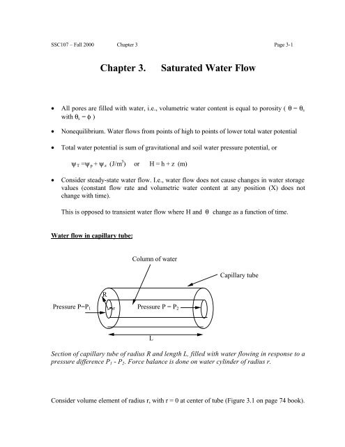
<strong>Water</strong> flow in capillary tube:<br />
Column of water<br />
Capillary tube<br />
R<br />
Pressure P=P 1 rr Pressure P = P 2<br />
L<br />
Section of capillary tube of radius R and length L, filled with water flowing in response to a<br />
pressure difference P 1 - P 2 . Force balance is done on water cylinder of radius r.<br />
Consider volume element of radius r, with r = 0 at center of tube (Figure <strong>3.</strong>1 on page 74 book).
SSC107 – Fall 2000 <strong>Chapter</strong> 3 Page 3-2<br />
Pressure difference across tube = P 1 - P 2 (N/m 2 ).<br />
Do force balance on cylindrical water volume with r radius r < R.<br />
Pressure force across two ends = (P 1 - P 2 ).A = ∆P πr 2<br />
Shear force on external area of water volume = τ(2πrL)<br />
Equating these 2 forces leads to: τ = ∆Pr/2L<br />
Earlier we found that τ = -υ dv/dr<br />
Equate and put terms with r together on left-hand side and integrate from r to R (v=0):<br />
rdr = - 2L υ<br />
∆P dv<br />
R<br />
∫<br />
r<br />
rdr = -2L υ<br />
∆P<br />
0<br />
∫<br />
v<br />
dv<br />
∆<br />
yields v(r)=<br />
P<br />
4L ( R 2 - r 2<br />
υ<br />
)<br />
When plotting velocity as a function of radius r, its distribution is parabolic:<br />
R<br />
Radial<br />
position, r<br />
0 <strong>Water</strong> velocity v(r ) v max<br />
✪ For which value of r is the water velocity at its maximum ?
SSC107 – Fall 2000 <strong>Chapter</strong> 3 Page 3-3<br />
At r = 0, where v = v max = R 2 ∆P/4Lν<br />
To find volumetric flow rate Q (volume per unit time), we must integrate v(r) over the area of<br />
the cylinder. Use cylindrical coordinates:<br />
Q =<br />
∫ ∫ v(r)dA<br />
Yielding Q =<br />
4<br />
π R ∆P<br />
8Lυ<br />
Using flow rate per unit area (water flux)<br />
J = R<br />
2<br />
2<br />
∆P<br />
R ρ g H<br />
K<br />
H w<br />
∆ ∆<br />
w<br />
[ = = ]<br />
8Lυ<br />
8Lν<br />
L<br />
NOTE: This equation is known as Poiseuille's law (<strong>Water</strong> flux is a function of pore radius)<br />
✪ Would you expect differences in flow rates between sands and clays, and if so why<br />
?<br />
In 1856, Darcy found for flow through saturated sand that<br />
Q = V ∆ H<br />
and is proportional to<br />
t<br />
∆ X<br />
Q - discharge rate ( volume water per time )<br />
V - volume of H O<br />
t - time<br />
X - distance or position<br />
∆H<br />
∆X<br />
- Total head gradient<br />
A gradient is the change of some parameter with position.<br />
2
SSC107 – Fall 2000 <strong>Chapter</strong> 3 Page 3-4<br />
The gradient should really be taken as an infinitesimal small change,<br />
notation)<br />
dH<br />
dX<br />
(differential<br />
Volume of H 2 O flowing through soil will be dependent upon area, hence<br />
Divide Q by A to describe flow on a relative basis:<br />
Q<br />
A = J<br />
w<br />
3<br />
⎡ m<br />
m s or m ⎤<br />
⎢<br />
⎣ s<br />
⎥<br />
⎦<br />
Q<br />
A = J = V At<br />
2 w<br />
J w - flux density (flux),<br />
which is proportional to<br />
∆H<br />
∆X<br />
The proportionality constant between flux and gradient is K, the hydraulic conductivity,<br />
or<br />
∆<br />
J w is proportional to K<br />
H ∆X<br />
For saturated sand, Darcy found that K was constant. Thus,<br />
J w = K<br />
∆H<br />
∆X<br />
✪ Can you now relate the Darcy flow equation with Poiseuille’s law ?<br />
What sign? + or -
SSC107 – Fall 2000 <strong>Chapter</strong> 3 Page 3-5<br />
Consider a horizontal soil column, saturated with water:<br />
water<br />
h p<br />
2<br />
1 Soil column<br />
Reference level (z=0)<br />
X = X 1 X = X 2<br />
H 1 = h p H 2 = 0<br />
And plot the change of total head (H) with position (X):<br />
H 1 = h p<br />
H<br />
Then:<br />
H 2 =0<br />
X<br />
X 1 X 2<br />
2 1<br />
J w = K H - H<br />
2 1<br />
X - X<br />
H<br />
X<br />
<<br />
H<br />
2 1<br />
><br />
X<br />
2 1<br />
(Note: Only in this example)<br />
Thus, ∆ H<br />
∆X is negative.<br />
For above case, J w would be negative, whereas flow is from left to right<br />
- Since flow is towards the right or towards larger X, it would
SSC107 – Fall 2000 <strong>Chapter</strong> 3 Page 3-6<br />
be logical to have J w be positive.<br />
- Put minus sign in front, so that:<br />
J w = - K<br />
So that flux is positive, if water is moving towards increasing X, or H is<br />
decreasing as X is increasing .<br />
∆H<br />
∆X<br />
Directional Convention for position (X)and flux density (J w )<br />
+<br />
- +<br />
Convention for locating variables is dependent on column orientation<br />
-<br />
horizontal vertical<br />
X 1 left (x 1 ) bottom (z 1 )<br />
X 2 right (x 2 ) top (z 2 )<br />
H 1 left bottom<br />
H 2 right top<br />
NOTE: In this class when using Darcy's Law and other similar transport equations,<br />
use this convention<br />
✪ When using this convention correctly, what is the sign of J w if water flow is
SSC107 – Fall 2000 <strong>Chapter</strong> 3 Page 3-7<br />
downward, upward, left or right ?<br />
J w = + flow to right or up<br />
J w = - flow to left or down<br />
The proper sign of J w is your self-check of the problem. Remember if H 2 > H 1 , water flows<br />
from position 2 towards position 1.<br />
The value of GRAVITATIONAL HEAD (z) depends on where you select the reference<br />
level. Above the reference level it is positive, below it is negative.<br />
EXAMPLES:<br />
A. Steady state saturated flow in horizontal soil columns<br />
water<br />
L<br />
b<br />
1 Soil column<br />
2<br />
Reference level (z=0)<br />
X 1 = x 1 = 0 X 2 = x 2 = L<br />
h 1 = b h 2 = 0<br />
H 1 = b H 2 = 0
SSC107 – Fall 2000 <strong>Chapter</strong> 3 Page 3-8<br />
Steady state is achieved when the flux of water out of the column is constant over time. If<br />
we could measure the flux at several cross sections at each point in the column, its value<br />
must be constant (flux of water in column = flux of water out column; hence there is no<br />
water storage change at any location in the column).<br />
J w = - K dH<br />
dX<br />
2 1<br />
= - K H - H<br />
X - X<br />
2 1<br />
= - K 0 - b<br />
L<br />
= Kb<br />
L<br />
And thus water flow is from left to right !!!<br />
✪ In which direction would water flow if the total head gradient is reversed ???<br />
L<br />
Reference level<br />
1 2<br />
Soil column<br />
X 1 = x 1 = 0 X 2 = x 2 = L<br />
h 1 = 0 h 2 = b<br />
H 1 = 0 H 2 = b<br />
b<br />
J w = - K dH<br />
dX<br />
= - K H - H<br />
2 1<br />
X 2 - X = - K b -0<br />
1 L<br />
= - Kb<br />
L<br />
If the head gradient is reversed; water flow is from right to left !!!!!!
SSC107 – Fall 2000 <strong>Chapter</strong> 3 Page 3-9<br />
B. Vertical soil columns:<br />
b<br />
2 X 2 = z 2 =L ; h 2 = b ; H 2 = L+b<br />
L soil J K dH K H<br />
w<br />
= − = −<br />
dX X<br />
downward flow<br />
− H<br />
− X<br />
2 1<br />
2 1<br />
K b +<br />
= −<br />
L<br />
L<br />
1 X 1 = z 1 =0 ; h 1 = 0 ; H 1 = 0<br />
When head gradient is reversed:<br />
2 X 2 = z 2 =L ; h 2 = 0 ; H 2 = L<br />
b L soil<br />
1<br />
J K dH K H<br />
w<br />
= − = −<br />
dX X<br />
− H<br />
− X<br />
2 1<br />
2 1<br />
K L − b K b −<br />
= −<br />
L =<br />
L L<br />
upward flow (J w >0)<br />
X 1 = z 1 =0 (reference level) ; h 1 = b ; H 1 = b<br />
NOTE: X-directional convention is independent of gravity reference<br />
✪ Compute the flux density, if one assumes the reference level at top of the column.
SSC107 – Fall 2000 <strong>Chapter</strong> 3 Page 3-10<br />
How does the total head change with position, if the soil is uniform?<br />
Consider the DARCY equation and note that it assumes that flow is steady state:<br />
J w = - K dH<br />
dX<br />
• Time does not appear in Darcy equation<br />
• Hence, flux (J w ) is constant<br />
• And q and h (or H) do not change with time<br />
• K is constant, because soil is uniform<br />
Then, for a uniform soil dH/dX is constant, and it can be shown that therefore H varies<br />
linearly with position X (straight line).<br />
✪ Proof that H varies linearly with X for a uniform soil.<br />
dH/dX is constant, or dH/dX = C 1<br />
Integrate: ∫ dH = C1∫<br />
dX<br />
Or: H = C 1 X + C 2 , for which the values of C 1 and C 2 depend on the values<br />
of H at the column ends.
SSC107 – Fall 2000 <strong>Chapter</strong> 3 Page 3-11<br />
<strong>Saturated</strong> Conductivity Measurement:<br />
(Constant Head Method)<br />
b level 2<br />
L soil X<br />
h z H<br />
level 1<br />
45 o<br />
0 b L L+b<br />
z, h, and H<br />
Draw z-line, which is a 1:1-line (slope is 45 o ).<br />
Draw H-line by adding z to h at any position X where both h and z are known.<br />
h 1 = 0 z 1 = 0 H 1 = 0 X 1 = 0<br />
h 2 = b z 2 = L H 2 = b+L X 2 = L<br />
Also h varies linearly with X.<br />
Applying Darcy's flow equation, and solve for K s (saturated hydraulic conductivity):<br />
2 1<br />
J w = Q s<br />
A = - K H - H<br />
2 1<br />
X - X<br />
= - K b + L<br />
s<br />
L<br />
K s = -<br />
QL<br />
A(L+ b)
SSC107 – Fall 2000 <strong>Chapter</strong> 3 Page 3-12<br />
<strong>Saturated</strong> flow in layered soils:<br />
b<br />
soil 2 L 2<br />
L 3<br />
2<br />
h 2 = b z 2 = L X 2 = L H 2 = b+L<br />
h 3 = ? z 3 = L 1 X 3 = L 1 H 3 = ?+L 1<br />
soil 1 L 1<br />
h 1 = 0 z 1 = 0 X 1 =0 H 1 = 0<br />
1<br />
✪ If K s -values for soil layers 1 and 2 are known, compute the soil water pressure<br />
head at the interface of the two layers (position 3).<br />
Steady-state:<br />
3 1<br />
J w = = - K H - H<br />
1<br />
X - X<br />
3 1<br />
= - K H - H<br />
2<br />
2 3<br />
2 1<br />
eff<br />
X 2 - X = - K H - H<br />
3 X 2 - X 1<br />
• Solve for H 3 , and subsequently for h 3<br />
• Check that J w (layer 1) = J w (layer 2)
SSC107 – Fall 2000 <strong>Chapter</strong> 3 Page 3-13<br />
From electical analog: R = ∆V/I (electrical resistance), we can write for hydraulic resistance<br />
(R H ) for each soil layer i:<br />
For each layer i:<br />
R<br />
H ,i<br />
=<br />
potential difference ∆Hi<br />
= = Li<br />
/Ki<br />
, from Darcy equation<br />
flux J<br />
where ∆H i denote the total head difference across layer i.<br />
Remember from electrical theory that the total resistance is equal to the sum of the individual<br />
resistances when in series. Hence, for the total layered soil system (with n layers), we can then<br />
define the effective hydraulic resistance (R H,eff )<br />
w<br />
∑ =<br />
R H,eff = R H,i<br />
n<br />
∑<br />
i = 1<br />
Li<br />
K i<br />
Also, we define: R<br />
H , eff =<br />
L<br />
K<br />
eff<br />
So that we can compute the effective hydraulic conductivity for the layered soil system (K eff )<br />
by equating the two above expressions (See book, page 84):<br />
K eff =<br />
L<br />
i<br />
∑<br />
L<br />
K i<br />
✪ Explain how we can apply the effective hydraulic conductivity concept to compute<br />
the steady state flux by knowing the total head values at the top and the bottom of a<br />
multi-layered soil column, and the thickness and saturated hydraulic conductivity<br />
values of each individual layer.
SSC107 – Fall 2000 <strong>Chapter</strong> 3 Page 3-14<br />
Falling head method to measure the saturated hydraulic conductivity of uniform soil:<br />
This method is used if it is expected that K s is low<br />
water<br />
b(t)<br />
2<br />
Position 2: z 2 =L ; h 2 = b(t) ; H 2 = L+b(t)<br />
L<br />
1<br />
Position 1: z 1 =0 ; h 1 = 0 ; H 2 = 0<br />
• The soil is saturated and has an unknown saturated hydraulic conductivity value, K s<br />
• The head of water on top of the soil column decreases with time (t), and is equal to b(t)<br />
• For uniform size column, the flux coming out of the column is:<br />
J<br />
w<br />
db<br />
K b ( t ) +<br />
= = −<br />
L<br />
s<br />
dt L<br />
Or:<br />
db( t)<br />
K<br />
sdt<br />
= − , where b=b 0 at t=0 and b=b 1 at t=t 1<br />
b( t) + L L<br />
• Integrate and solve for K s at time t 1 : K<br />
s<br />
=<br />
L ⎡b<br />
ln⎢<br />
t ⎣ b<br />
o<br />
1 1<br />
+<br />
+<br />
L⎤<br />
⎥<br />
L ⎦<br />
✪ Special assignment: Derive the expression for K s , if the area of the water-filled<br />
tube (a) is much smaller than the area of the soil column (A)