Introductory Differential Equations using Sage - William Stein

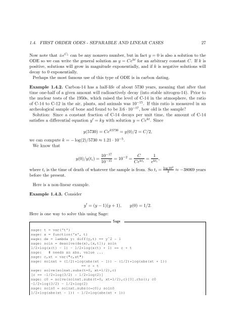
1.4. FIRST ORDER ODES - SEPARABLE AND LINEAR CASES 27
Now note that ±e C 1
can be any nonzero number, but in fact y = 0 is also a solution to the
ODE so we can write the general solution as y = Ce kt for an arbitrary constant C. If k is
positive, solutions will grow in magnitude exponentially, and if k is negative solutions will
decay to 0 exponentially.
Perhaps the most famous use of this type of ODE is in carbon dating.
Example 1.4.2. Carbon-14 has a half-life of about 5730 years, meaning that after that
time one-half of a given amount will radioactively decay (into stable nitrogen-14). Prior to
the nuclear tests of the 1950s, which raised the level of C-14 in the atmosphere, the ratio
of C-14 to C-12 in the air, plants, and animals was 10 −15 . If this ratio is measured in an
archeological sample of bone and found to be 3.6 · 10 −17 , how old is the sample?
Solution: Since a constant fraction of C-14 decays per unit time, the amount of C-14
satisfies a differential equation y ′ = ky with solution y = Ce kt . Since
y(5730) = Ce k5730 = y(0)/2 = C/2,
we can compute k = − log(2)/5730 ≈ 1.21 · 10 −5 .
We know that
y(0)/y(t i ) = 10−17
10 −15 = 10−2 = C
Ce kt i = 1
e kt i ,
where t i is the time of death of whatever the sample is from. So t i =
before the present.
Here is a non-linear example.
Example 1.4.3. Consider
Here is one way to solve this using Sage:
y ′ = (y − 1)(y + 1), y(0) = 1/2.
Sage
log 102
k
≈ −38069 years
sage: t = var(’t’)
sage: x = function(’x’, t)
sage: de = lambda y: diff(y,t) == yˆ2 - 1
sage: soln = desolve(de(x),[x,t]); soln
1/2*log(x(t) - 1) - 1/2*log(x(t) + 1) == c + t
sage: # needs an abs. value ...
sage: c,xt = var("c,xt")
sage: solnxt = (1/2)*log(abs(xt - 1)) - (1/2)*log(abs(xt + 1))
== c + t
sage: solve(solnxt.subs(t=0, xt=1/2),c)
[c == -1/2*log(3/2) - 1/2*log(2)]
sage: c0 = solve(solnxt.subs(t=0, xt=1/2),c)[0].rhs(); c0
-1/2*log(3/2) - 1/2*log(2)
sage: soln0 = solnxt.subs(c=c0); soln0
1/2*log(abs(xt - 1)) - 1/2*log(abs(xt + 1))