Introductory Differential Equations using Sage - William Stein

Introductory Differential Equations using Sage 

David Joyner 

Marshall Hampton 

2010-11-11

v 

There are some things which cannot 

be learned quickly, and time, which is all we have, 

must be paid heavily for their acquiring. 

They are the very simplest things, 

and because it takes a man’s life to know them 

the little new that each man gets from life 

is very costly and the only heritage he has to leave. 

Ernest Hemingway 

(From A. E. Hotchner, Papa Hemingway, Random House, NY, 1966)

Contents 

1 First order differential equations 3 

1.1 Introduction to DEs . . . . . . . . . . . . . . . . . . . . . . . . . . . . . . . 3 

1.2 Initial value problems . . . . . . . . . . . . . . . . . . . . . . . . . . . . . . 11 

1.3 Existence of solutions to ODEs . . . . . . . . . . . . . . . . . . . . . . . . . 16 

1.3.1 First order ODEs . . . . . . . . . . . . . . . . . . . . . . . . . . . . . 16 

1.3.2 Higher order constant coefficient linear homogeneous ODEs . . . . . 20 

1.4 First order ODEs - separable and linear cases . . . . . . . . . . . . . . . . . 22 

1.4.1 Separable DEs . . . . . . . . . . . . . . . . . . . . . . . . . . . . . . 22 

1.4.2 Autonomous ODEs . . . . . . . . . . . . . . . . . . . . . . . . . . . . 26 

1.4.3 Substitution methods . . . . . . . . . . . . . . . . . . . . . . . . . . 28 

1.4.4 Linear 1st order ODEs . . . . . . . . . . . . . . . . . . . . . . . . . . 29 

1.5 Isoclines and direction fields . . . . . . . . . . . . . . . . . . . . . . . . . . . 32 

1.6 Numerical solutions - Euler’s method and improved Euler’s method . . . . . 37 

1.6.1 Euler’s Method . . . . . . . . . . . . . . . . . . . . . . . . . . . . . . 37 

1.6.2 Improved Euler’s method . . . . . . . . . . . . . . . . . . . . . . . . 39 

1.6.3 Euler’s method for systems and higher order DEs . . . . . . . . . . . 41 

1.7 Numerical solutions II - Runge-Kutta and other methods . . . . . . . . . . 43 

1.7.1 Fourth-Order Runge Kutta method . . . . . . . . . . . . . . . . . . 44 

1.7.2 Multistep methods - Adams-Bashforth . . . . . . . . . . . . . . . . . 45 

1.7.3 Adaptive step size . . . . . . . . . . . . . . . . . . . . . . . . . . . . 46 

1.8 Newtonian mechanics . . . . . . . . . . . . . . . . . . . . . . . . . . . . . . 48 

1.9 Application to mixing problems . . . . . . . . . . . . . . . . . . . . . . . . . 52 

2 Second order differential equations 57 

2.1 Linear differential equations . . . . . . . . . . . . . . . . . . . . . . . . . . . 57 

2.2 Linear differential equations, continued . . . . . . . . . . . . . . . . . . . . . 61 

2.3 Undetermined coefficients method . . . . . . . . . . . . . . . . . . . . . . . 66 

2.3.1 Simple case . . . . . . . . . . . . . . . . . . . . . . . . . . . . . . . . 67 

2.3.2 Non-simple case . . . . . . . . . . . . . . . . . . . . . . . . . . . . . 69 

2.3.3 Annihilator method . . . . . . . . . . . . . . . . . . . . . . . . . . . 72 

2.4 Variation of parameters . . . . . . . . . . . . . . . . . . . . . . . . . . . . . 75 

2.4.1 The Leibniz rule . . . . . . . . . . . . . . . . . . . . . . . . . . . . . 75 

2.4.2 The method . . . . . . . . . . . . . . . . . . . . . . . . . . . . . . . . 76 

vii

viii 

CONTENTS 

2.5 Applications of DEs: Spring problems . . . . . . . . . . . . . . . . . . . . . 78 

2.5.1 Part 1 . . . . . . . . . . . . . . . . . . . . . . . . . . . . . . . . . . . 78 

2.5.2 Part 2 . . . . . . . . . . . . . . . . . . . . . . . . . . . . . . . . . . . 82 

2.5.3 Part 3 . . . . . . . . . . . . . . . . . . . . . . . . . . . . . . . . . . . 85 

2.6 Applications to simple LRC circuits . . . . . . . . . . . . . . . . . . . . . . 87 

2.7 The power series method . . . . . . . . . . . . . . . . . . . . . . . . . . . . . 92 

2.7.1 Part 1 . . . . . . . . . . . . . . . . . . . . . . . . . . . . . . . . . . . 92 

2.7.2 Part 2 . . . . . . . . . . . . . . . . . . . . . . . . . . . . . . . . . . . 97 

2.8 The Laplace transform method . . . . . . . . . . . . . . . . . . . . . . . . . 101 

2.8.1 Part 1 . . . . . . . . . . . . . . . . . . . . . . . . . . . . . . . . . . . 101 

2.8.2 Part 2 . . . . . . . . . . . . . . . . . . . . . . . . . . . . . . . . . . . 108 

2.8.3 Part 3 . . . . . . . . . . . . . . . . . . . . . . . . . . . . . . . . . . . 115 

3 Matrix theory and systems of DEs 117 

3.1 Row reduction and solving systems of equations . . . . . . . . . . . . . . . . 117 

3.1.1 The Gauss elimination game . . . . . . . . . . . . . . . . . . . . . . 117 

3.1.2 Solving systems using inverses . . . . . . . . . . . . . . . . . . . . . 120 

3.1.3 Solving higher-dimensional linear systems . . . . . . . . . . . . . . . 124 

3.2 Quick survey of linear algebra . . . . . . . . . . . . . . . . . . . . . . . . . . 125 

3.2.1 Matrix arithmetic . . . . . . . . . . . . . . . . . . . . . . . . . . . . 125 

3.2.2 Determinants . . . . . . . . . . . . . . . . . . . . . . . . . . . . . . . 129 

3.2.3 Vector spaces . . . . . . . . . . . . . . . . . . . . . . . . . . . . . . . 130 

3.2.4 Bases, dimension, linear independence and span . . . . . . . . . . . . 131 

3.2.5 The Wronskian . . . . . . . . . . . . . . . . . . . . . . . . . . . . . . 134 

3.3 Application: Solving systems of DEs . . . . . . . . . . . . . . . . . . . . . . 134 

3.3.1 Modeling battles using Lanchester’s equations . . . . . . . . . . . . . 137 

3.3.2 Romeo and Juliet . . . . . . . . . . . . . . . . . . . . . . . . . . . . . 143 

3.3.3 Electrical networks using Laplace transforms . . . . . . . . . . . . . 148 

3.4 Eigenvalue method for systems of DEs . . . . . . . . . . . . . . . . . . . . . 152 

3.5 Introduction to variation of parameters for systems . . . . . . . . . . . . . . 163 

3.5.1 Motivation . . . . . . . . . . . . . . . . . . . . . . . . . . . . . . . . 163 

3.5.2 The method . . . . . . . . . . . . . . . . . . . . . . . . . . . . . . . . 164 

3.6 Nonlinear systems . . . . . . . . . . . . . . . . . . . . . . . . . . . . . . . . 168 

3.6.1 Linearizing near equilibria . . . . . . . . . . . . . . . . . . . . . . . . 169 

3.6.2 The nonlinear pendulum . . . . . . . . . . . . . . . . . . . . . . . . . 170 

3.6.3 The Lorenz equations . . . . . . . . . . . . . . . . . . . . . . . . . . 172 

3.6.4 Zombies attack . . . . . . . . . . . . . . . . . . . . . . . . . . . . . . 173 

4 Introduction to partial differential equations 175 

4.1 Introduction to separation of variables . . . . . . . . . . . . . . . . . . . . . 175 

4.2 Fourier series, sine series, cosine series . . . . . . . . . . . . . . . . . . . . . 179 

4.3 The heat equation . . . . . . . . . . . . . . . . . . . . . . . . . . . . . . . . 186 

4.3.1 Method for zero ends . . . . . . . . . . . . . . . . . . . . . . . . . . . 187 

4.3.2 Method for insulated ends . . . . . . . . . . . . . . . . . . . . . . . . 188

CONTENTS 

ix 

4.3.3 Explanation . . . . . . . . . . . . . . . . . . . . . . . . . . . . . . . . 192 

4.4 The wave equation in one dimension . . . . . . . . . . . . . . . . . . . . . . 195 

5 Appendices 207 

5.1 Appendix: Integral table . . . . . . . . . . . . . . . . . . . . . . . . . . . . . 208

CONTENTS 

xi 

Preface 

The majority of this book came from lecture notes David Joyner (WDJ) typed up over the 

years for a course on differential equations with boundary value problems at the US Naval 

Academy (USNA). Though the USNA is a government institution and official work-related 

writing is in the public domain, so much of this was done at home during the night and 

weekends that he feels he has the right to claim copyright over this work. The DE course at 

the USNA has used various editions of the following three books (in order of most common 

use to least common use) at various times: 

• Dennis G. Zill and Michael R. Cullen, Differential equations with Boundary 

Value Problems, 6th ed., Brooks/Cole, 2005. 

• R. Nagle, E. Saff, and A. Snider, Fundamentals of Differential Equations and 

Boundary Value Problems, 4th ed., Addison/Wesley, 2003. 

• W. Boyce and R. DiPrima, Elementary Differential Equations and Boundary 

Value Problems, 8th edition, John Wiley and Sons, 2005. 

You may see some similarities but, for the most part, WDJ has taught things a bit differently 

and tried to impart this in these notes. Time will tell if there are any improvements. 

After WDJ finished a draft of this book, he invited the second author, Marshall Hampton 

(MH), to revise and extend it. At the University of Minnesota Duluth, MH teaches a course 

on differential equations and linear algebra. 

A new feature to this book is the fact that every section has at least one Sage exercise. 

Sage is FOSS (free and open source software), available on the most common computer 

platforms. Royalties for the sales of this book (if it ever makes it’s way to a publisher) will 

go to further development of Sage . 

Some exercises in the text are considerably more challenging than others. We have indicated 

these with an asterisk in front of the exercise number. 

This book is free and open source. It is licensed under the Attribution-ShareAlike Creative 

Commons license, http://creativecommons.org/licenses/by-sa/3.0/, or the Gnu 

Free Documentation License (GFDL), http://www.gnu.org/copyleft/fdl.html, at 

your choice. 

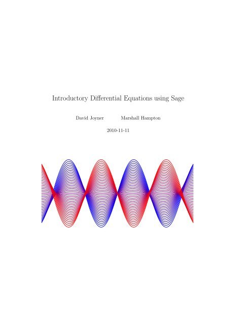
The cover image was created with the following Sage code: 

from math import cos, sin 

def RK4(f, t_start, y_start, t_end, steps): 

’’’ 

fourth-order Runge-Kutta solver with fixed time steps. 

f must be a function of t,y. 

’’’ 

step_size = (t_end - t_start)/steps 

t_current = t_start 

argn = len(y_start) 

y_current = [x for x in y_start] 

Sage

xii 

CONTENTS 

answer_table = [] 

answer_table.append([t_current,y_current]) 

for j in range(0,steps): 

k1=f(t_current,y_current) 

k2=f(t_current+step_size/2,[y_current[i] + k1[i]*step_size/2 for i in range(argn)]) 

k3=f(t_current+step_size/2,[y_current[i] + k2[i]*step_size/2 for i in range(argn)]) 

k4=f(t_current+step_size,[y_current[i] + k3[i]*step_size for i in range(argn)]) 

t_current += step_size 

y_current = [y_current[i] + (step_size/6)*(k1[i]+2*k2[i]+2*k3[i]+k4[i]) for i in range(len(k1))] 

answer_table.append([t_current,y_current]) 

return answer_table 

def e1(t, y): 

return [-y[1],sin(y[0])] 

npi = N(pi) 

sols = [] 

for v in srange(-1,1+.04,.05): 

p1 = RK4(e1,0.0,[0.0,v],-2.5*npi,200)[::-1] 

p1 = p1 + RK4(e1,0.0,[0.0,v],2.5*npi,200) 

sols.append(list_plot([[x[0],x[1][0]] for x in p1], plotjoined=True, rgbcolor = ((v+1)/2.01,0,(1.01-v)/2.01))) 

f = 2 

show(sum(sols), axes = True, figsize = [f*5*npi/3,f*2.5], xmin = -7, xmax = 7, ymin = -1, ymax = 1)

CONTENTS 1 

Acknowledgments 

In a few cases we have made use of the excellent (public domain!) lecture notes by Sean 

Mauch, Introduction to methods of Applied Mathematics, available online at 

http://www.its.caltech.edu/~sean/book/unabridged.html (as of Fall, 2009). 

In some cases, we have made use of the material on Wikipedia - this includes both discussion 

and in a few cases, diagrams or graphics. This material is licensed under the GFDL or 

the Attribution-ShareAlike Creative Commons license. In any case, the amount used here 

probably falls under the “fair use” clause. 

Software used: 

Most of the graphics in this text was created using Sage (http://www.sagemath.org/) 

and GIMP http://www.gimp.org/ by the authors. The most important components of 

Sage for our purposes are: Maxima, SymPy and Matplotlib. The circuit diagrams were created 

using Dia http://www.gnome.org/projects/dia/ and GIMP by the authors. A few 

diagrams were “taken” from Wikipedia http://www.wikipedia.org/ (and acknowledged 

in the appropriate placein the text). Of course, L A TEX was used for the typesetting. Many 

thanks to the developers of these programs for these free tools.

2 CONTENTS

Chapter 1 

First order differential equations 

But there is another reason for the high repute of mathematics: it is mathematics 

that offers the exact natural sciences a certain measure of security which, 

without mathematics, they could not attain. 

- Albert Einstein 

1.1 Introduction to DEs 

Roughly speaking, a differential equation is an equation involving the derivatives of one 

or more unknown functions. Implicit in this vague definition is the assumption that the 

equation imposes a constraint on the unknown function (or functions). For example, we 

would not call the well-known product rule identity of differential calculus a differential 

equation. 

dx 

Example 1.1.1. Here is a simple example of a differential equation: 

dt 

= x. A solution 

would be a function x(t) which is differentiable on some interval and whose derivative is 

equal to itself. Can you guess any solutions? 

In calculus (differential-, integral- and vector-), you’ve studied ways of analyzing functions. 

You might even have been convinced that functions you meet in applications arise naturally 

from physical principles. As we shall see, differential equations arise naturally from general 

physical principles. In many cases, the functions you met in calculus in applications to 

physics were actually solutions to a naturally-arising differential equation. 

Example 1.1.2. Consider a falling body of mass m on which exactly three forces act: 

• gravitation, F grav , 

• air resistance, F res , 

• an external force, F ext = f(t), where f(t) is some given function. 

3

4 CHAPTER 1. FIRST ORDER DIFFERENTIAL EQUATIONS 

✻ 

F res 

mass m 

❄ 

F grav 

Let x(t) denote the distance fallen from some fixed initial position. The velocity is denoted 

by v = x ′ and the acceleration by a = x ′′ . We choose an orientation so that downwards is 

positive. In this case, F grav = mg, where g > 0 is the gravitational constant. We assume 

that air resistance is proportional to velocity (a common assumption in physics), and write 

F res = −kv = −kx ′ , where k > 0 is a “friction constant”. The total force, F total , is by 

hypothesis, 

and, by Newton’s 2nd Law 1 , 

F total = F grav + F res + F ext , 

Putting these together, we have 

F total = ma = mx ′′ . 

or 

mx ′′ = ma = mg − kx ′ + f(t), 

mx ′′ + kx ′ = f(t) + mg. 

This is a differential equation in x = x(t). It may also be rewritten as a differential equation 

in v = v(t) = x ′ (t) as 

mv ′ + kv = f(t) + mg. 

This is an example of a “first order differential equation in v”, which means that at most 

first order derivatives of the unknown function v = v(t) occur. 

In fact, you have probably seen solutions to this in your calculus classes, at least when 

f(t) = 0 and k = 0. In that case, v ′ (t) = g and so v(t) = ∫ g dt = gt+C. Here the constant 

of integration C represents the initial velocity. 

Differential equations occur in other areas as well: weather prediction (more generally, 

fluid-flow dynamics), electrical circuits, the temperature of a heated homogeneous wire, and 

many others (see the table below). They even arise in problems on Wall Street: the Black- 

Scholes equation is a PDE which models the pricing of derivatives [BS-intro]. Learning to 

solve differential equations helps you understand the behaviour of phenomenon present in 

these problems. 

1 “Force equals mass times acceleration.” http://en.wikipedia.org/wiki/Newtons_law

1.1. INTRODUCTION TO DES 5 

phenomenon 

weather 

falling body 

motion of a mass attached 

to a spring 

motion of a plucked guitar string 

Battle of Trafalger 

cooling cup of coffee 

in a room 

population growth 

description of DE 

Navier-Stokes equation [NS-intro] 

a non-linear vector-valued higher-order PDE 

1st order linear ODE 

Hooke’s spring equation 

2nd order linear ODE [H-intro] 

Wave equation 

2nd order linear PDE [W-intro] 

Lanchester’s equations 

system of 2 1st order DEs [L-intro], [M-intro], [N-intro] 

Newton’s Law of Cooling 

1st order linear ODE 

logistic equation 

non-linear, separable, 1st order ODE 

Undefined terms and notation will be defined below, except for the equations themselves. 

For those, see the references or wait until later sections when they will be introduced 2 . 

Basic Concepts: 

Here are some of the concepts to be introduced below: 

• dependent variable(s), 

• independent variable(s), 

• ODEs, 

• PDEs, 

• order, 

• linearity, 

• solution. 

It is really best to learn these concepts using examples. However, here are the general 

definitions anyway, with examples to follow. 

The term “differential equation” is sometimes abbreviated DE, for brevity. 

Dependent/independent variables: Put simply, a differential equation is an equation 

involving derivatives of one of more unknown functions. The variables you are differentiating 

with respect to are the independent variables of the DE. The variables (the “unknown 

functions”) you are differentiating are the dependent variables of the DE. Other variables 

which might occur in the DE are sometimes called “parameters”. 

2 Except for the important Navier-Stokes equation, which is relatively complicated and would take us too 

far afield, http://en.wikipedia.org/wiki/Navier-stokes.


ODE/PDE: If none of the derivatives which occur in the DE are partial derivatives (for 

example, if the dependent variable/unknown function is a function of a single variable) 

then the DE is called an ordinary differential equation or ODE. If some of the derivatives 

which occur in the DE are partial derivatives then the DE is a partial differential 

equation or PDE. 

Order: The highest total number of derivatives you have to take in the DE is it’s order. 

Linearity: This can be described in a few different ways. First of all, a DE is linear if 

the only operations you perform on its terms are combinations of the following: 

• differentiation with respect to independent variable(s), 

• multiplication by a function of the independent variable(s). 

Another way to define linearity is as follows. A linear ODE having independent variable 

t and the dependent variable is y is an ODE of the form 

a 0 (t)y (n) + ... + a n−1 (t)y ′ + a n (t)y = f(t), 

for some given functions a 0 (t), ..., a n (t), and f(t). Here 

y (n) = y (n) (t) = dn y(t) 

dt n 

denotes the n-th derivative of y = y(t) with respect to t. The terms a 0 (t), ..., a n (t) are 

called the coefficients of the DE and we will call the term f(t) the non-homogeneous 

term or the forcing function. (In physical applications, this term usually represents an 

external force acting on the system. For instance, in the example above it represents the 

gravitational force, mg.) 

Solution: An explicit solution to a DE having independent variable t and the dependent 

variable is x is simple a function x(t) for which the DE is true for all values of t. 

Here are some examples: 

Example 1.1.3. Here is a table of examples. As an exercise, determine which of the 

following are ODEs and which are PDEs.


DE indep vars dep vars order linear? 

mx ′′ + kx ′ = mg t x 2 yes 

falling body 

mv ′ + kv = mg t v 1 yes 

falling body 

k ∂2 u 

= ∂u 

∂x 2 

∂t 

t, x u 2 yes 

heat equation 

mx ′′ + bx ′ + kx = f(t) t x 2 yes 

spring equation 

P ′ = k(1− P )P t P 1 no 

K 

logistic population equation 

k ∂2 u 

= ∂2 u 

∂x 2 

t, x u 2 yes 

∂ 2 t 

wave equation 

T ′ = k(T− T room) t T 1 yes 

Newton’s Law of Cooling 

x ′ =−Ay, y ′ =−Bx, t x, y 1 yes 

Lanchester’s equations 

Remark 1.1.1. Note that in many of these examples, the symbol used for the independent 

variable is not made explicit. For example, we are writing x ′ when we really mean x ′ (t) = 

x(t) 

dt 

. This is very common shorthand notation and, in this situation, we shall usually use t 

as the independent variable whenever possible. 

Example 1.1.4. Recall a linear ODE having independent variable t and the dependent 

variable is y is an ODE of the form 

a 0 (t)y (n) + ... + a n−1 (t)y ′ + a n (t)y = f(t), 

for some given functions a 0 (t), ..., a n (t), and f(t). The order of this DE is n. In particular, 

a linear 1st order ODE having independent variable t and the dependent variable is y is an 

ODE of the form 

a 0 (t)y ′ + a 1 (t)y = f(t), 

for some a 0 (t), a 1 (t), and f(t). We can divide both sides of this equation by the leading 

coefficient a 0 (t) without changing the solution y to this DE. Let’s do that and rename the 

terms: 

y ′ + p(t)y = q(t), 

where p(t) = a 1 (t)/a 0 (t) and q(t) = f(t)/a 0 (t). Every linear 1st order ODE can be put into 

this form, for some p and q. For example, the falling body equation mv ′ + kv = f(t) + mg 

has this form after dividing by m and renaming v as y. 

What does a differential equation like mx ′′ + kx ′ = mg or P ′ = k(1 − P K )P or k ∂2 u 

∂ 2 t 

really mean? In mx ′′ + kx ′ = mg, m and k and g are given constants. The only things that 

can vary are t and the unknown function x = x(t). 

∂x 2 = ∂2 u


Example 1.1.5. To be specific, let’s consider x ′ +x = 1. This means for all t, x ′ (t)+x(t) = 

1. In other words, a solution x(t) is a function which, when added to its derivative you 

always get the constant 1. How many functions are there with that property? Try guessing 

a few “random” functions: 

• Guess x(t) = sin(t). Compute (sin(t)) ′ + sin(t) = cos(t) + sin(t) = √ 2sin(t + π 4 ). 

x ′ (t) + x(t) = 1 is false. 

• Guess x(t) = exp(t) = e t . Compute (e t ) ′ + e t = 2e t . x ′ (t) + x(t) = 1 is false. 

• Guess x(t) = exp(t) = t 2 . Compute (t 2 ) ′ + t 2 = 2t + t 2 . x ′ (t) + x(t) = 1 is false. 

• Guess x(t) = exp(−t) = e −t . Compute (e −t ) ′ + e −t = 0. x ′ (t) + x(t) = 1 is false. 

• Guess x(t) = exp(t) = 1. Compute (1) ′ + 1 = 0 + 1 = 1. x ′ (t) + x(t) = 1 is true. 

We finally found a solution by considering the constant function x(t) = 1. Here a way of 

doing this kind of computation with the aid of the computer algebra system Sage: 

Sage 

sage: t = var(’t’) 

sage: de = lambda x: diff(x,t) + x - 1 

sage: de(sin(t)) 

sin(t) + cos(t) - 1 

sage: de(exp(t)) 

2*eˆt - 1 

sage: de(tˆ2) 

tˆ2 + 2*t - 1 

sage: de(exp(-t)) 

-1 

sage: de(1) 

0 

Note we have rewritten x ′ + x = 1 as x ′ + x − 1 = 0 and then plugged various functions for 

x to see if we get 0 or not. 

Obviously, we want a more systematic method for solving such equations than guessing 

all the types of functions we know one-by-one. We will get to those methods in time. First, 

we need some more terminology. 

IVP: A first order initial value problem (abbreviated IVP) is a problem of the form 

x ′ = f(t,x), x(a) = c, 

where f(t,x) is a given function of two variables, and a, c are given constants. The equation 

x(a) = c is the initial condition. 

Under mild conditions of f, an IVP has a solution x = x(t) which is unique. This means 

that if f and a are fixed but c is a parameter then the solution x = x(t) will depend on c. 

This is stated more precisely in the following result.


Theorem 1.1.1. (Existence and uniqueness) Fix a point (t 0 ,x 0 ) in the plane. Let f(t,x) 

be a function of t and x for which both f(t,x) and f x (t,x) = ∂f(t,x) 

∂x 

are continuous on some 

rectangle 

a < t < b, c < x < d, 

in the plane. Here a,b,c,d are any numbers for which a < t 0 

there is an h > 0 and a unique solution x = x(t) for which 

and x(t 0 ) = x 0 . 

x ′ = f(t,x), for all t ∈ (t 0 − h,t 0 + h), 

This is proven in §2.8 of Boyce and DiPrima [BD-intro], but we shall not prove this here 

(though we will return to it in more detail in §1.3 below). In most cases we shall run across, 

it is easier to construct the solution than to prove this general theorem. 

Example 1.1.6. Let us try to solve 

x ′ + x = 1, x(0) = 1. 

The solutions to the DE x ′ +x = 1 which we “guessed at” in the previous example, x(t) = 1, 

satisfies this IVP. 

Here a way of finding this solution with the aid of the computer algebra system Sage: 



sage: x = function(’x’, t) 

sage: de = lambda y: diff(y,t) + y - 1 

sage: desolve(de(x),[x,t],[0,1]) 

1 

(The command desolve is a DE solver in Sage.) Just as an illustration, let’s try another 

example. Let us try to solve 

x ′ + x = 1, x(0) = 2. 

The Sage commands are similar: 




sage: de = lambda y: diff(y,t) + y - 1 

sage: x0 = 2 # this is for the IC x(0) = 2 

sage: soln = desolve(de(x),[x,t],[0,x0]) 

sage: solnx = lambda s: RR(soln.subs(t=s))


sage: P = plot(solnx,0,5) 

sage: soln; show(P) 

(eˆt + 1)*eˆ(-t) 

This gives the solution x(t) = (e t + 1)e −t = 1 + e −t and the plot given in Figure 1.1. 

Figure 1.1: Solution to IVP x ′ + x = 1, x(0) = 2. 

Example 1.1.7. Now let us consider an example which does not satisfy all of the assumptions 

of the existence and uniqueness theorem: x ′ = x 2/3 . The function x = (t/3 + C) 3 is a 

solution to this differential equation for any choice of the constant C. If we consider only 

solutions with the initial value x(0) = 0, we see that we can choose C = 0 - i.e. x = t 3 /27 

satisfies the differential equation and has x(0) = 0. But there is another solution with that 

initial condition - the solution x = 0. So a solutions exist, but they are not necessarily 

unique. 

Some conditions on the ODE which guarantee a unique solution will be presented in §1.3. 

Exercises: 

1. Verify that y = 2e −3x is a solution to the differential equation y ′ = −3y. 

2. Verify that x = t 3 + 5 is a solution to the differential equation x ′ = 3t 2 . 

3. Subsitute x = e rt into the differential equation x ′′ + x ′ − 6x = 0 and determine all 

values of the parameter r which give a solution. 

4. (a) Verify the, for any constant c, the function x(t) = 1+ce −t solves x ′ + x = 1. Find 

the c for which this function solves the IVP x ′ + x = 1, x(0) = 3. 

(b) Solve

1.2. INITIAL VALUE PROBLEMS 11 

using Sage. 

x ′ + x = 1, x(0) = 3, 

5. Write a differential equation for a population P that is changing in time (t) such that 

the rate of change is proportional to the square root of P. 

1.2 Initial value problems 

Recall, 1 st order initial value problem, or IVP, is simply a 1 st order ODE and an initial 

condition. For example, 

x ′ (t) + p(t)x(t) = q(t), x(0) = x 0 , 

where p(t), q(t) and x 0 are given. The analog of this for 2 nd order linear DEs is this: 

a(t)x ′′ (t) + b(t)x ′ (t) + c(t)x(t) = f(t), x(0) = x 0 , x ′ (0) = v 0 , 

where a(t), b(t), c(t), x 0 , and v 0 are given. This 2 nd order linear DE and initial conditions 

is an example of a 2 nd order IVP. In general, in an IVP, the number of initial conditions 

must match the order of the DE. 

Example 1.2.1. Consider the 2 nd order DE 

x ′′ + x = 0. 

(We shall run across this DE many times later. As we will see, it represents the displacement 

of an undamped spring with a unit mass attached. The term harmonic oscillator is 

attached to this situation [O-ivp].) Suppose we know that the general solution to this DE 

is 

x(t) = c 1 cos(t) + c 2 sin(t), 

for any constants c 1 , c 2 . This means every solution to the DE must be of this form. (If 

you don’t believe this, you can at least check it it is a solution by computing x ′′ (t) + x(t) 

and verifying that the terms cancel, as in the following Sage example. Later, we see how to 

derive this solution.) Note that there are two degrees of freedom (the constants c 1 and c 2 ), 

matching the order of the DE. 



sage: c1 = var(’c1’) 


sage: de = lambda x: diff(x,t,t) + x 

sage: de(c1*cos(t) + c2*sin(t)) 

0 

sage: x = function(’x’, t)


sage: soln = desolve(de(x),[x,t]); soln 

k1*sin(t) + k2*cos(t) 

sage: solnx = lambda s: RR(soln.subs(k1=1, k2=0, t=s)) 

sage: P = plot(solnx,0,2*pi) 

sage: show(P) 

This is displayed in Figure 1.2. 

Now, to solve the IVP 

x ′′ + x = 0, x(0) = 0, x ′ (0) = 1. 

the problem is to solve for c 1 and c 2 for which the x(t) satisfies the initial conditions. The 

two degrees of freedom in the general solution matching the number of initial conditions in 

the IVP. Plugging t = 0 into x(t) and x ′ (t), we obtain 

0 = x(0) = c 1 cos(0) + c 2 sin(0) = c 1 , 1 = x ′ (0) = −c 1 sin(0) + c 2 cos(0) = c 2 . 

Therefore, c 1 = 0, c 2 = 1 and x(t) = sin(t) is the unique solution to the IVP. 

Figure 1.2: Solution to IVP x ′′ + x = 0, x(0) = 0, x ′ (0) = 1. 

In Figure 1.2, you see the solution oscillates, as t increases. 

Another example, 


x ′′ + 4x ′ + 4x = 0. 

(We shall run across this DE many times later as well. As we will see, it represents the 

displacement of a critially damped spring with a unit mass attached.) Suppose we know 

that the general solution to this DE is 

x(t) = c 1 exp(−2t) + c 2 t exp(−2t) = c 1 e −2t + c 2 te −2t , 

for any constants c 1 , c 2 . This means every solution to the DE must be of this form. (Again, 

you can at least check it is a solution by computing x ′′ (t), 4x ′ (t), 4x(t), adding them up 

and verifying that the terms cancel, as in the following Sage example.)






sage: de = lambda x: diff(x,t,t) + 4*diff(x,t) + 4*x 

sage: de(c1*exp(-2*t) + c2*t*exp(-2*t)) 

0 

sage: desolve(de(x),[x,t]) 

(k2*t + k1)*eˆ(-2*t) 

sage: P = plot(t*exp(-2*t),0,pi) 

sage: show(P) 

The plot is displayed in Figure 1.3. 

Now, to solve the IVP 

x ′′ + 4x ′ + 4x = 0, x(0) = 0, x ′ (0) = 1. 

we solve for c 1 and c 2 using the initial conditions. Plugging t = 0 into x(t) and x ′ (t), we 

obtain 

0 = x(0) = c 1 exp(0) + c 2 · 0 · exp(0) = c 1 , 

1 = x ′ (0) = c 1 exp(0) + c 2 exp(0) − 2c 2 · 0 · exp(0) = c 1 + c 2 . 

Therefore, c 1 = 0, c 1 + c 2 = 1 and so x(t) = t exp(−2t) is the unique solution to the IVP. 

In Figure 1.3, you see the solution tends to 0, as t increases. 

Figure 1.3: Solution to IVP x ′′ + 4x ′ + 4x = 0, x(0) = 0, x ′ (0) = 1. 

Suppose, for the moment, that for some reason you mistakenly thought that the general 

solution to this DE was


x(t) = c 1 exp(−2t) + c 2 exp(−2t) = e −2t (c 1 + c 2 ), 

for arbitray constants c 1 , c 2 . (Note: the “extra t-factor” on the second term on the right is 

missing from this expression.) Now, if you try to solve for the constant c 1 and c 2 using the 

initial conditions x(0) = 0, x ′ (0) = 1 you will get the equations 

c 1 + c 2 = 0 

−2c 1 − 2c 2 = 1. 

These equations are impossible to solve! The moral of the story is that you must have a 

correct general solution to insure that you can always solve your IVP. 

One more quick example. 


x ′′ − x = 0. 

Suppose we know that the general solution to this DE is 

x(t) = c 1 exp(t) + c 2 exp(−t) = c 1 e t + c 2 e −t , 

for any constants c 1 , c 2 . (Again, you can check it is a solution.) 

The solution to the IVP 

x ′′ − x = 0, x(0) = 1, x ′ (0) = 0, 

is x(t) = et +e −t 

2 

. (You can solve for c 1 and c 2 yourself, as in the examples above.) This particular 

function is also called a hyperbolic cosine function, denoted cosh(t) (pronounced 

“kosh”). The hyperbolic sine function, denoted sinh(t) (pronounced “sinch”), satisfies 

the IVP 

x ′′ − x = 0, x(0) = 0, x ′ (0) = 1. 

The hyperbolic trig functions have many properties analogous to the usual trig functions 

and arise in many areas of applications [H-ivp]. For example, cosh(t) represents a catenary 

or hanging cable [C-ivp]. 





sage: de = lambda x: diff(x,t,t) - x 

sage: de(c1*exp(-t) + c2*exp(-t)) 

0 

sage: desolve(de(x)),[x,t])


k1*eˆt + k2*eˆ(-t) 

sage: P = plot(eˆt/2-eˆ(-t)/2,0,3) 

sage: show(P) 

Figure 1.4: Solution to IVP x ′′ − x = 0, x(0) = 0, x ′ (0) = 1. 

You see in Figure 1.4 that the solution tends to infinity, as t gets larger. 

Exercises: 

1. Find the value of the constant C that makes x = Ce 3t a solution to the IVP x ′ = 3x, 

x(0) = 4. 

2. Verify that x = (C+t)cos(t) satisfies the differential equation x ′ +xtan(t)−cos(t) = 0 

and find the value of C that gives the initial condition x(2π) = 0. 

3. Determine a value of the constant C so that the given solution of the differential 

equation satisfies the initial condition. 

(a) y = ln(x + C) solves e y y ′ = 1, y(0) = 1. 

(b) y = Ce −x + x − 1 solves y ′ = x − y, y(0) = 3. 

4. Use Sage to check that the general solution to the falling body problem 

mv ′ + kv = mg, 

is v(t) = mg 

k 

+ ce−kt/m . If v(0) = v 0 , you can solve for c in terms of v 0 to get 

c = v 0 − mg 

k . Take m = k = v 0 = 1, g = 9.8 and use Sage to plot v(t) for 0 < t < 1.


5. Consider a spacecraft falling towards the moon at a speed of 500 m/s (meters per 

second) at a height of 50 km. Assume the moon’s acceleration on the spacecraft is 

a constant −1.63 m/s 2 . When the spacecraft’s rockets are engaged, the total acceleration 

on the rocket (gravity+rocket thrust) is 3 m/s 2 . At what height should the 

rockets be engaged so that the spacecraft lands at zero velocity? 

1.3 Existence of solutions to ODEs 

When do solutions to an ODE exist? When are they unique? This section gives some 

necessary conditions for determining existence and uniqueness. 

1.3.1 First order ODEs 

We begin by considering the first order initial value problem 

x ′ (t) = f(t,x(t)), x(a) = c. (1.1) 

What conditions on f (and a and c) guarantee that a solution x = x(t) exists? If it exists, 

what (further) conditions guarantee that x = x(t) is unique? 

The following result addresses the first question. 

Theorem 1.3.1. (“Peano’s existence theorem” [P-intro]) Suppose f is bounded and continuous 

in x, and t. Then, for some value ǫ > 0, there exists a solution x = x(t) to the 

initial value problem within the range [a − ǫ,a + ǫ]. 

Giuseppe Peano (1858 - 1932) was an Italian mathematician, who is mostly known for 

his important work on the logical foundations of mathematics. For example, the common 

notations for union ∪ and intersections ∩ first appeared in his first book dealing with 

mathematical logic, written while he was teaching at the University of Turin. 

Example 1.3.1. Take f(x,t) = x 2/3 . This is continuous and bounded in x and t in 

−1 < x < 1, t ∈ R. The IVP x ′ = f(x,t), x(0) = 0 has two solutions, x(t) = 0 and 

x(t) = t 3 /27. 

You all know what continuity means but you may not be familiar with the slightly stronger 

notion of “Lipschitz continuity”. This is defined next. 

Definition 1.3.1. Let D ⊂ R 2 be a domain. A function f : D → R is called Lipschitz 

continuous if there exists a real constant K > 0 such that, for all x 1 ,x 2 ∈ D, 

|f(x 1 ) − f(x 2 )| ≤ K|x 1 − x 2 |. 

The smallest such K is called the Lipschitz constant of the function f on D. 

For example, 

• the function f(x) = x 2/3 defined on [−1,1] is not Lipschitz continuous;

1.3. EXISTENCE OF SOLUTIONS TO ODES 17 

• the function f(x) = x 2 defined on [−3,7] is Lipschitz continuous, with Lipschitz 

constant K = 14; 

• the function f defined by f(x) = x 3/2 sin(1/x) (x ≠ 0) and f(0) = 0 restricted to 

[0,1], gives an example of a function that is differentiable on a compact set while not 

being Lipschitz. 

Theorem 1.3.2. (“Picard’s existence and uniqueness theorem” [PL-intro]) Suppose f is 

bounded, Lipschitz continuous in x, and continuous in t. Then, for some value ǫ > 0, 

there exists a unique solution x = x(t) to the initial value problem (1.1) within the range 

[a − ǫ,a + ǫ]. 

Charles Émile Picard (1856-1941) was a leading French mathematician. Picard made his 

most important contributions in the fields of analysis, function theory, differential equations, 

and analytic geometry. In 1885 Picard was appointed to the mathematics faculty at the 

Sorbonne in Paris. Picard was awarded the Poncelet Prize in 1886, the Grand Prix des 

Sciences Mathmatiques in 1888, the Grande Croix de la Légion d’Honneur in 1932, the 

Mittag-Leffler Gold Medal in 1937, and was made President of the International Congress 

of Mathematicians in 1920. He is the author of many books and his collected papers run to 

four volumes. 

The proofs of Peano’s theorem or Picard’s theorem go well beyond the scope of this course. 

However, for the curious, a very brief indication of the main ideas will be given in the sketch 

below. For details, see an advanced text on differential equations. 

sketch or the idea of the proof: A simple proof of existence of the solution is obtained by 

successive approximations. In this context, the method is known as Picard iteration. 

Set x 0 (t) = c and 

x i (t) = c + 

∫ t 

a 

f(s,x i−1 (s))ds. 

It turns out that Lipschitz continuity implies that the mapping T defined by 

T(y)(t) = c + 

∫ t 

a 

f(s,y(s))ds, 

is a contraction mapping on a certain Banach space. It can then be shown, by using the 

Banach fixed point theorem, that the sequence of “Picard iterates” x i is convergent and 

that the limit is a solution to the problem. The proof of uniqueness uses a result called 

Grönwall’s Lemma. □ 

Example 1.3.2. Consider the IVP 

x ′ = 1 − x, x(0) = 1, 

with the constant solution x(t) = 1. Computing the Picard iterates by hand is easy: 

x 0 (t) = 1, x 1 (t) = 1+ ∫ t 

0 1 −x 0(s))ds = 1, x 2 (t) = 1+ ∫ t 

0 1 −x 1(s))ds = 1, and so on. Since 

each x i (t) = 1, we find the solution


x(t) = lim 

i→∞ 

x i (t) = lim 

i→∞ 

1 = 1. 

We now try the Picard iteration method in Sage . Consider the IVP 

x ′ = 1 − x, x(0) = 2, 

which we considered earlier. 


sage: var(’t, s’) 

sage: f = lambda t,x: 1-x 

sage: a = 0; c = 2 

sage: x0 = lambda t: c; x0(t) 

2 

sage: x1 = lambda t: c + integral(f(s,x0(s)), s, a, t); x1(t) 

2 - t 


tˆ2/2 - t + 2 


-tˆ3/6 + tˆ2/2 - t + 2 


tˆ4/24 - tˆ3/6 + tˆ2/2 - t + 2 


-tˆ5/120 + tˆ4/24 - tˆ3/6 + tˆ2/2 - t + 2 


tˆ6/720 - tˆ5/120 + tˆ4/24 - tˆ3/6 + tˆ2/2 - t + 2 

sage: P1 = plot(x2(t), t, 0, 2, linestyle=’--’) 

sage: P2 = plot(x4(t), t, 0, 2, linestyle=’-.’) 

sage: P3 = plot(x6(t), t, 0, 2, linestyle=’:’) 

sage: P4 = plot(1+exp(-t), t, 0, 2) 

sage: (P1+P2+P3+P4).show() 

From the graph in Figure 1.5 you can see how well these iterates are (or at least appear to 

be) converging to the true solution x(t) = 1 + e −t . 

More generally, here is some Sage code for Picard iteration. 


def picard_iteration(f, a, c, N): 

’’’ 

Computes the N-th Picard iterate for the IVP 

x’ = f(t,x), x(a) = c. 

EXAMPLES: 

sage: var(’x t s’) 

(x, t, s) 

sage: a = 0; c = 2 

sage: f = lambda t,x: 1-x


Figure 1.5: Picard iteration for x ′ = 1 − x, x(0) = 2. 

sage: picard_iteration(f, a, c, 0) 

2 


2 - t 


tˆ2/2 - t + 2 


-tˆ3/6 + tˆ2/2 - t + 2 

’’’ 

if N == 0: 

return c*t**0 

if N == 1: 

x0 = lambda t: c + integral(f(s,c*s**0), s, a, t) 

return expand(x0(t)) 

for i in range(N): 

x_old = lambda s: picard_iteration(f, a, c, N-1).subs(t=s) 

x0 = lambda t: c + integral(f(s,x_old(s)), s, a, t) 

return expand(x0(t)) 

Exercises: 

1. Compute the first three Picard iterates for the IVP 

x ′ = 1 + xt, x(0) = 0


using the initial function x 0 (t) = 0. 

2. Apply the Picard iteration method in Sage to the IVP 

and find the first three iterates. 

x ′ = (t + x) 2 , x(0) = 2, 

1.3.2 Higher order constant coefficient linear homogeneous ODEs 

We begin by considering the second order 3 initial value problem 

ax ′′ + bx ′ + cx = 0, x(0) = d 0 , x ′ (0) = d 1 , (1.2) 

where a,b,c,d 0 ,d 1 are constants and a ≠ 0. What conditions guarantee that a solution 

x = x(t) exists? If it exists, what (further) conditions guarantee that x = x(t) is unique? 

It turns out that no conditions are needed - a solution to 1.2 always exists and is unique. 

As we will see later, we can construct distinct explicit solutions, denoted x 1 = x 1 (t) and 

x 2 = x 2 (t) and sometimes called fundamental solutions, to ax ′′ + bx ′ + cx = 0. If we 

let x = c 1 x 1 + c 2 x 2 , for any constants c 1 and c 2 , then we know that x is also a solution 4 , 

sometimes called the general solution to ax ′′ + bx ′ + cx = 0. But how do we know there 

exist c 1 and c 2 for which this general solution also satisfies the initial conditions x(0) = d 0 

and x ′ (0) = d 1 ? For this to hold, we need to be able to solve 

c 1 x 1 (0) + c 2 x 2 (0) = d 1 , c 1 x ′ 1(0) + c 2 x ′ 2(0) = d 2 , 

for c 1 and c 2 . By Cramer’s rule, 

∣ d ∣ 1 x 2 (0) ∣∣∣ 

d 2 x ′ 2 

c 1 = 

(0) ∣ x 1(0) d 1 

x ′ 1 ∣ x ∣, c 

1(0) x 2 (0) ∣∣∣ 2 = 

(0) d ∣ 

2 

x ′ 1 (0) x′ 2 (0) ∣ x ∣. 

1(0) x 2 (0) ∣∣∣ 

x ′ 1 (0) x′ 2 (0) 

For this solution to exist, the denominators in these quotients must be non-zero. This 

denominator is the value of the “Wronskian” [W-linear] at t = 0. 

Definition 1.3.2. For n functions f 1 , ..., f n , which are n − 1 times differentiable on an 

interval I, the Wronskian W(f 1 ,...,f n ) as a function on I is defined by 

for x ∈ I. 

W(f 1 ,... ,f n )(x) = 

∣ 

f 1 (x) f 2 (x) · · · f n (x) 

f 1 ′(x) f 2 ′(x) · · · f n ′ (x) 

. 

. . .. , . 

1 

(x) f (n−1) 

2 

(x) · · · f n 

(n−1) 

(x) ∣ 

f (n−1) 

3 It turns out that the reasoning in the second order case is very similar to the general reasoning for n-th 

order DEs. For simplicity of presentation, we restrict to the 2-nd order case. 

4 This follows form the linearity assumption.


The matrix constructed by placing the functions in the first row, the first derivative of 

each function in the second row, and so on through the (n − 1)-st derivative, is a square 

matrix sometimes called a fundamental matrix of the functions. The Wronskian is the 

determinant of the fundamental matrix. 

Theorem 1.3.3. (“Abel’s identity”) Consider a homogeneous linear second-order ordinary 

differential equation 

d 2 y 

dx 2 + p(x)dy dx + q(x)y = 0 

on the real line with a continuous function p. The Wronskian W of two solutions of the 

differential equation satisfies the relation 

( ∫ x 

) 

W(x) = W(0)exp − P(s)ds . 

Example 1.3.3. Consider x ′′ + 3x ′ + 2x = 0. The Sage code below calculates the Wronskian 

of the two fundamental solutions e −t and e −2t both directly and from Abel’s identity 

(Theorem 1.3.3). 

sage: t = var("t") 

sage: x = function("x",t) 

sage: DE = diff(x,t,t)+3*diff(x,t)+2*x==0 

sage: desolve(DE, [x,t]) 

k1*eˆ(-t) + k2*eˆ(-2*t) 

sage: Phi = matrix([[eˆ(-t), eˆ(-2*t)],[-eˆ(-t), -2*eˆ(-2*t)]]); Phi 

[ eˆ(-t) eˆ(-2*t)] 

[ -eˆ(-t) -2*eˆ(-2*t)] 

sage: W = det(Phi); W 

-eˆ(-3*t) 

sage: Wt = eˆ(-integral(3,t)); Wt 

eˆ(-3*t) 

sage: W*W(t=0) == Wt 

eˆ(-3*t) == eˆ(-3*t) 

sage: bool(W*W(t=0) == Wt) 

True 


0 

Definition 1.3.3. We say n functions f 1 , ..., f n are linearly dependent over the interval 

I, if there are numbers a 1 , · · · ,a n (not all of them zero) such that 

a 1 f 1 (x) + · · · + a n f n (x) = 0, 

for x ∈ I. If the functions are not linearly dependent then they are called linearly independent.


Theorem 1.3.4. If the Wronskian is non-zero at some point in an interval, then the associated 

functions are linearly independent on the interval. 

Example 1.3.4. If f 1 (t) = e t and f 2 (t) = e −t then 

Indeed, 

sage: var(’t’) 

t 

sage: f1 = exp(t); f2 = exp(-t) 

sage: wronskian(f1,f2) 

-2 

∣ ∣ et e −t ∣∣∣ 

e t −e −t = −2. 


Therefore, the fundamental solutions x 1 = e t , x 2 = e −t are 

Exercises: 

1. Using Sage, verify Abel’s identity 

(a) in the example x ′′ − x = 0, 

(b) in the example x ′′ + 2 ∗ x ′ + 2x = 0. 

Determine what the existence and uniqueness theorem (Theorem 1 from Chapter 1.3) 

guarantees about solutions to the following initial value problems (note that you do 

not have to find the solutions): 

2. dy/dx = √ xy, y(0) = 1. 

3. dy/dx = y 1/3 , y(0) = 2. 

4. dy/dx = y 1/3 , y(2) = 0. 

5. dy/dx = xln(y), y(0) = 1. 

1.4 First order ODEs - separable and linear cases 

1.4.1 Separable DEs 

We know how to solve any ODE of the form 

y ′ = f(t),

1.4. FIRST ORDER ODES - SEPARABLE AND LINEAR CASES 23 

at least in principle - just integrate both sides 5 . For a more general type of ODE, such as 

y ′ = f(t,y), 

this fails. For instance, if y ′ = t + y then integrating both sides gives y(t) = ∫ dy 

∫ dt dt = 

y ′ dt = ∫ t+y dt = ∫ t dt+ ∫ y(t)dt = t2 2 +∫ y(t)dt. So, we have only succeeded in writing 

y(t) in terms of its integral. Not very helpful. 

However, there is a class of ODEs where this idea works, with some modification. If the 

ODE has the form 

then it is called separable 6 . 

To solve a separable ODE: 

y ′ = g(t) 

h(y) , (1.3) 

(1) write the ODE (1.3) as dy 

dt = g(t) 

h(y) , 

(2) “separate” the t’s and the y’s: 

(3) integrate both sides: 

h(y)dy = g(t)dt, 

∫ 

∫ 

h(y)dy = 

g(t)dt + C (1.4) 

I’ve added a “+C” to emphasize that a constant of integration must be included in 

your answer (but only on one side of the equation). 

The answer obtained in this manner is called an “implicit solution” of (1.3) since it 

expresses y implicitly as a function of t. 

Why does this work? It is easiest to understand by working backwards from the formula 

(1.4). Recall that one form of the fundamental theorem of calculus is d ∫ 

dy h(y)dy = h(y). 

If we think of y as a being a function of t, and take the t-derivative, we can use the chain 

rule to get 

g(t) = d dt 

∫ 

g(t)dt = d dt 

∫ 

h(y)dy = ( d ∫ 

dy 

h(y)dy) dy 

dt = h(y)dy dt . 

So if we differentiate both sides of equation (1.4) with respect to t, we recover the original 

differential equation. 

5 Recall y ′ really denotes dy 

dt , so by the fundamental theorem of calculus, y = R dy 

dt dt = R y ′ dt = R f(t)dt = 

F(t) + c, where F is the “anti-derivative” of f and c is a constant of integration. 

6 It particular, any separable DE must be first order, ordinary differential equation.


Example 1.4.1. Are the following ODEs separable? If so, solve them. 

(a) (t 2 + y 2 )y ′ = −2ty, 

(b) y ′ = −x/y, y(0) = −1, 

(c) T ′ = k · (T − T room ), where k < 0 and T room are constants, 

(d) ax ′ + bx = c, where a ≠ 0, b ≠ 0, and c are constants 

(e) ax ′ + bx = c, where a ≠ 0, b, are constants and c = c(t) is not a constant. 

(f) y ′ = (y − 1)(y + 1), y(0) = 2. 

(g) y ′ = y 2 + 1, y(0) = 1. 

Solutions: 

(a) not separable, 

(b) y dy = −xdx, so y 2 /2 = −x 2 /2+c, so x 2 +y 2 = 2c. This is the general solution (note 

it does not give y explicitly as a function of x, you will have to solve for y algebraically 

to get that). The initial conditions say when x = 0, y = 1, so 2c = 0 2 + 1 2 = 1, which 

gives c = 1/2. Therefore, x 2 + y 2 = 1, which is a circle. That is not a function so 

cannot be the solution we want. The solution is either y = √ 1 − x 2 or y = − √ 1 − x 2 , 

but which one? Since y(0) = −1 (note the minus sign) it must be y = − √ 1 − x 2 . 

(c) 

dT 

T −T room 

= kdt, so ln |T − T room | = kt + c (some constant c), so T − T room = Ce kt 

(some constant C), so T = T(t) = T room + Ce kt . 

(d) dx 

dt = (c − bx)/a = − b a (x − c dx 

b 

), so 

x− c b 

= − b a dt, so ln |x − c b | = − b at + C, where C is a 

constant of integration. This is the implicit general solution of the DE. The explicit 

general solution is x = c b + Be− b a t , where B is a constant. 

The explicit solution is easy find using Sage: 


sage: a = var(’a’) 

sage: b = var(’b’) 

sage: c = var(’c’) 



sage: de = lambda y: a*diff(y,t) + b*y - c 


(c*eˆ(b*t/a)/b + c)*eˆ(-b*t/a)


(e) If c = c(t) is not constant then ax ′ + bx = c is not separable. 

(f) 

dy 

(y−1)(y+1) = dt so 1 2 

(ln(y −1)−ln(y+1)) = t+C, where C is a constant of integration. 

This is the “general (implicit) solution” of the DE. 

Note: the constant functions y(t) = 1 and y(t) = −1 are also solutions to this DE. 

These solutions cannot be obtained (in an obvious way) from the general solution. 

The integral is easy to do using Sage: 


sage: y = var(’y’) 

sage: integral(1/((y-1)*(y+1)),y) 

log(y - 1)/2 - (log(y + 1)/2) 

Now, let’s try to get Sage to solve for y in terms of t in 1 2 

(ln(y −1)−ln(y+1)) = t+C: 


sage: C = var(’C’) 

sage: solve([log(y - 1)/2 - (log(y + 1)/2) == t+C],y) 

[log(y + 1) == -2*C + log(y - 1) - 2*t] 

This is not working. Let’s try inputting the problem in a different form: 


sage: C = var(’C’) 

sage: solve([log((y - 1)/(y + 1)) == 2*t+2*C],y) 

[y == (-eˆ(2*C + 2*t) - 1)/(eˆ(2*C + 2*t) - 1)] 

This is what we want. Now let’s assume the initial condition y(0) = 2 and solve for 

C and plot the function. 


sage: solny=lambda t:(-eˆ(2*C+2*t)-1)/(eˆ(2*C+2*t)-1) 

sage: solve([solny(0) == 2],C) 

[C == log(-1/sqrt(3)), C == -log(3)/2] 

sage: C = -log(3)/2 

sage: solny(t) 

(-eˆ(2*t)/3 - 1)/(eˆ(2*t)/3 - 1) 

sage: P = plot(solny(t), 0, 1/2) 

sage: show(P)


This plot is shown in Figure 1.6. The solution has a singularity at t = ln(3)/2 = 

0.5493.... 

Figure 1.6: Plot of y ′ = (y − 1)(y + 1), y(0) = 2, for 0 < t < 1/2. 

(g) 

dy 

y 2 +1 

= dt so arctan(y) = t + C, where C is a constant of integration. The initial 

condition y(0) = 1 says arctan(1) = C, so C = π 4 . Therefore y = tan(t + π 4 

) is the 

solution. 

1.4.2 Autonomous ODEs 

A special subclass of separable ODEs is the class of autonomous ODEs, which have the 

form 

y ′ = f(y), 

where f is a given function (i.e., the slope y only depends on the value of the dependent 

variable y). The cases (c), (d), (f), and (g) above are examples. 

One of the simplest examples of an autonomous ODE is dy 

dt 

= ky, where k is a constant. 

We can divide by y and integrate to get 

∫ ∫ 

1 

y dy = log |y| = k dt = kt + C 1 . 

After exponentiating, we get 

|y| = e kt+C 1 

= e C 1 

e kt . 

We can drop the absolute value if we allow positive and negative solutions: 

y = ±e C 1 

e kt .


Now note that ±e C 1 

can be any nonzero number, but in fact y = 0 is also a solution to the 

ODE so we can write the general solution as y = Ce kt for an arbitrary constant C. If k is 

positive, solutions will grow in magnitude exponentially, and if k is negative solutions will 

decay to 0 exponentially. 

Perhaps the most famous use of this type of ODE is in carbon dating. 

Example 1.4.2. Carbon-14 has a half-life of about 5730 years, meaning that after that 

time one-half of a given amount will radioactively decay (into stable nitrogen-14). Prior to 

the nuclear tests of the 1950s, which raised the level of C-14 in the atmosphere, the ratio 

of C-14 to C-12 in the air, plants, and animals was 10 −15 . If this ratio is measured in an 

archeological sample of bone and found to be 3.6 · 10 −17 , how old is the sample? 

Solution: Since a constant fraction of C-14 decays per unit time, the amount of C-14 

satisfies a differential equation y ′ = ky with solution y = Ce kt . Since 

y(5730) = Ce k5730 = y(0)/2 = C/2, 

we can compute k = − log(2)/5730 ≈ 1.21 · 10 −5 . 

We know that 

y(0)/y(t i ) = 10−17 

10 −15 = 10−2 = C 

Ce kt i = 1 

e kt i , 

where t i is the time of death of whatever the sample is from. So t i = 

before the present. 

Here is a non-linear example. 

Example 1.4.3. Consider 

Here is one way to solve this using Sage: 

y ′ = (y − 1)(y + 1), y(0) = 1/2. 


log 102 

k 

≈ −38069 years 



sage: de = lambda y: diff(y,t) == yˆ2 - 1 

sage: soln = desolve(de(x),[x,t]); soln 

1/2*log(x(t) - 1) - 1/2*log(x(t) + 1) == c + t 

sage: # needs an abs. value ... 

sage: c,xt = var("c,xt") 

sage: solnxt = (1/2)*log(abs(xt - 1)) - (1/2)*log(abs(xt + 1)) 

== c + t 

sage: solve(solnxt.subs(t=0, xt=1/2),c) 

[c == -1/2*log(3/2) - 1/2*log(2)] 

sage: c0 = solve(solnxt.subs(t=0, xt=1/2),c)[0].rhs(); c0 

-1/2*log(3/2) - 1/2*log(2) 

sage: soln0 = solnxt.subs(c=c0); soln0 

1/2*log(abs(xt - 1)) - 1/2*log(abs(xt + 1))


== t - 1/2*log(3/2) -1/2*log(2) 

sage: implicit_plot(soln0,(t,-1/2,1/2),(xt,0,0.9)) 

Sage cannot solve this (implicit) solution for x(t), though I’m sure you can do it by hand if 

you want. The (implicit) plot is given in Figure 1.7. 

Figure 1.7: Plot of y ′ = (y − 1)(y + 1), y(0) = 1/2, for −1/2 < t < 1/2. 

A more complicated example is 

y ′ = y(y − 1)(y − 2). 

This has constant solutions y(t) = 0, y(t) = 1, and y(t) = 2. (Check this.) Several 

non-constant solutions are plotted in Figure 1.8. 

Exercise: Find the general solution to y ′ = y(y − 1)(y − 2) either “by hand” or using Sage 

. 

1.4.3 Substitution methods 

Sometimes it is possible to solve differential equations by substitution, just as some integrals 

can be simplified by substitution. 

Example 1.4.4. We will solve the ODE y ′ = (y+x+3) 2 with the substitution v = y+x+3. 

Differentiating the substitution gives the relation v ′ = y ′ +1, so the ODE can be rewritten 

as v ′ −1 = v 2 , or v ′ = v 2 +1. This transformed ODE is separable, so we divide by v 2 +1 and 

integrate to get arctan(v) = x + C. Taking the tangent of both sides gives v = tan(x + C) 

and now we substitute back to get y = tan(x + C) − x − 3.


2 

1.5 

1 

0.5 

1 2 3 4 

Figure 1.8: Plot of y ′ = y(y − 1)(y − 2), y(0) = y 0 , for 0 < t < 4, and various values of y 0 . 

There are a variety of very specialized substitution methods which we will not present in 

this text. However one class of differential equations is common enough to warrant coverage 

here: homogeneous ODEs. Unfortunately, for historical reasons the word homogeneous has 

come to mean two different things. In the present context, we define a homogeneous firstorder 

ODE to be one which can be written as y ′ = f(y/x). For example, the following ODE 

is homogeneous in this sense: 

dy 

dx = x/y. 

A first-order homogeneous ODE can be simplified by using the substitution v = y/x, or 

equivalently y = vx. Differentiating that relationship gives us v + xv ′ = y ′ . 

Example 1.4.5. We will solve the ODE y ′ = y/x + 2 with the substitution v = y/x. 

As noted above, with this substituion y ′ = v +xv ′ so the original ODE becomes v +xv ′ = 

v + 2. This simplifies to v ′ = 2/x which can be directly integrated to get v = 2log(x) + C 

(in more difficult examples we would get a separable ODE after the substitution). Using 

the substitution once again we obtain y/x = 2log(x) + C so the general solution is y = 

2xlog(x) + Cx. 

1.4.4 Linear 1st order ODEs 

The bottom line is that we want to solve any problem of the form 

x ′ + p(t)x = q(t), (1.5) 

where p(t) and q(t) are given functions (which, let’s assume, aren’t “too horrible”). Every 

first order linear ODE can be written in this form. Examples of DEs which have this form: 

Falling Body problems, Newton’s Law of Cooling problems, Mixing problems, certain simple 

Circuit problems, and so on.


There are two approaches 

• “the formula”, 

• the method of integrating factors. 

Both lead to the exact same solution. 

“The Formula”: The general solution to (1.5) is 

∫ R 

e 

p(t) dt 

q(t)dt + C 

x = 

, (1.6) 

e R p(t) dt 

where C is a constant. The factor e R p(t) dt is called the integrating factor and is often 

denoted by µ. This formula was apparently first discovered by Johann Bernoulli [F-1st]. 

Example 1.4.6. Solve 

xy ′ + y = e x . 

We rewrite this as y ′ + 1 x y = ex x . Now compute µ = eR 1 

x dx = e ln(x) = x, so the formula 

gives 

y = 

∫ 

x 

e x x dx + C 

x 

= 

∫ 

e x dx + C 

x 

= ex + C 

. 

x 

Here is one way to do this using Sage: 




sage: de = lambda y: diff(y,t) + (1/t)*y - exp(t)/t 


(c + eˆt)/t 

“Integrating factor method”: Let µ = e R p(t) dt . Multiply both sides of (1.5) by µ: 

The product rule implies that 

µx ′ + p(t)µx = µq(t). 

(µx) ′ = µx ′ + p(t)µx = µq(t). 

(In response to a question you are probably thinking now: No, this is not obvious. This is 

Bernoulli’s very clever idea.) Now just integrate both sides. By the fundamental theorem 

of calculus,


∫ 

µx = 

Dividing both side by µ gives (1.6). 

∫ 

(µx) ′ dt = 

µq(t)dt. 

Exercises: 

Find the general solution to the following seperable differential equations: 

1. x ′ = 2xt. 

2. x ′ − xsin(t) = 0 

3. (1 + t)x ′ = 2x. 

4. x ′ − xt − x = 1 + t. 

5. Find the solution y(x) to the following initial value problem: y ′ = 2ye x , y(0) = 2e 2 . 

6. Find the solution y(x) to the following initial value problem: y ′ = x 3 (y 2 +1), y(0) = 1. 

7. Use the substitution v = y/x to solve the IVP: y ′ = 2xy 

x 2 −y 2 , y(0) = 2. 

Solve the following linear equations. Find the general solution if no initial condition 

is given. 

8. x ′ + x = 1, x(0) = 0. 

9. x ′ + 4x = 2te −4t . 

10. tx ′ + 2x = 2t, x(1) = 1 2 . 

11. dy/dx + y tan(x) = sin(x). 

12. xy ′ = y + 2x, y(1) = 2. 

13. y ′ + 4y = 2xe −4x , y(0) = 0. 

14. y ′ = cos(x) − y cos(x), y(0) = 1. 

15. In carbon-dating organic material it is assumed that the amount of carbon-14 ( 14 C) 

decays exponentially ( d 14 C 

dt 

= −k 14 C) with rate constant of k ≈ 0.0001216 where 

t is measured in years. Suppose an archeological bone sample contains 1/7 as much 

carbon-14 as is in a present-day sample. How old is the bone? 

16. The function e −t2 does not have an anti-derivative in terms of elementary functions, 

but this anti-derivative is important in probability. So we define a new function, 

erf(t) := √ 2 ∫ u 

π 0 e−u2 du. Find the solution of x ′ − 2xt = 1 in terms of erf(t).


17. (a) Use Sage’s desolve command to solve 

tx ′ + 2x = e t /t. 

(b) Use Sage to plot the solution to y ′ = y 2 − 1, y(0) = 2. 

1.5 Isoclines and direction fields 

Recall from vector calculus the notion of a two-dimensional vector field: ⃗ F(x,y) = (g(x,y),h(x,y)). 

To plot ⃗ F, you simply draw the vector ⃗ F(x,y) at each point (x,y). 

The idea of the direction field (or slope field) associated to the first order ODE 

y ′ = f(x,y), y(a) = c, (1.7) 

is similar. At each point (x,y) you plot a small vector having slope f(x,y). For example, 

the vector field plot of ⃗ F(x,y) = (1,f(x,y)) or ⃗ F(x,y) = (1,f(x,y))/ √ 1 + f(x,y) 2 (which 

is a unit vector). 

How would you draw such a direction field plot by hand? You could compute the value of 

f(x,y) for lots and lots of points (x,y) nd then plot a tiny arrow of slope f(x,y) at each 

of these points. Unfortunately, this would be virtually impossible for a person to do if the 

number of points was large. 

For this reason, the notion of the “isoclines” of the ODE is very useful. An isocline of 

(1.7) is a level curve of the function z = f(x,y): 

{(x,y) | f(x,y) = m}, 

where the given constant m is called the slope of the isocline. In terms of the ODE, this 

curve represents the collection of all points (x,y) at which the solution has slope m. In 

terms of the direction field of the ODE, it represents the collection of points where the 

vectors have slope m. This means that once you have draw a single isocline, you can sketch 

ten or more tiny vectors describing your direction field. Very useful indeed! This idea is 

recoded below more algorithmically. 

How to draw the direction field of (1.7) by hand: 

• Draw several isoclines, making sure to include one which contains the point (a,c). 

(You may want to draw these in pencil.) 

• On each isocline, draw “hatch marks” or “arrows” along the line each having slope 

m. 

This is a crude direction field plot. The plot of arrows form your direction field. The 

isoclines, having served their usefulness, can now safely be ignored.

1.5. ISOCLINES AND DIRECTION FIELDS 33 

Example 1.5.1. The direction field, with three isoclines, for 

is given by the graph in Figure 1.9. 

y ′ = 5x + y − 5, y(0) = 1, 

Figure 1.9: Plot of y ′ = 5x + y − 5, y(0) = 1, for −1 < x < 1. 

The isoclines are the curves (coincidentally, lines) of the form 5x + y − 5 = m. These are 

lines of slope −5, not to be confused with the fact that it represents an isocline of slope m. 

The above example can be solved explicitly. (Indeed, y = −5x+e x solves y ′ = 5x+y −5, 

y(0) = 1.) In the next example, such an explicit solution is not possible. Therefore, a 

numerical approximation plays a more important role. 

Example 1.5.2. The direction field, with three isoclines, for 

is given by the in Figure 1.10. 

y ′ = x 2 + y 2 , y(0) = 3/2, 

The isoclines are the concentric circles x 2 + y 2 = m. 

The plot in Figure 1.10 was obtaining using the Sage code below. 

sage: x,y = var("x,y") 

sage: f(x,y) = xˆ2 + yˆ2 

sage: plot_slope_field(f(x,y), (x,-2,2),(y,-2,2)).show(aspect_ratio=1) 


There is also a way to “manually draw” these direction fields using Sage .


Figure 1.10: Direction field and solution plot of y ′ = x 2 + y 2 , y(0) = 3/2, for −2 < x < 2. 


sage: pts = [(-2+i/5,-2+j/5) for i in range(20) \ 

for j in range(20)] # square [-2,2]x[-2,2] 

sage: f = lambda p:p[0]ˆ2+p[1]ˆ2 # x = p[0] and y = p[1] 

sage: arrows = [arrow(p, (p[0]+0.02,p[1]+(0.02)*f(p)), \ 

width=1/100, rgbcolor=(0,0,1)) for p in pts] 

sage: show(sum(arrows)) 

This gives the plot in Figure 1.11. 

Figure 1.11: Direction field for y ′ = x 2 + y 2 , y(0) = 3/2, for −2 < x < 2.

1.5. ISOCLINES AND DIRECTION FIELDS 35 

Exercises: 

1. Match the solution curves in Figure 1.12 to the ODEs below. 

I. y ′ = y 2 − 1 

II. y ′ = y − 1 

t 2 

III. y ′ = sin(t)sin(y) 

IV. y ′ = sin(ty) 

V. y ′ = 2t + y 

VI. y ′ = sin(3t) 

2. Using Sage , plot the direction field for y ′ = x 2 − y 2 .


(a) 

(b) 

(c) 

(d) 

(e) 

(f) 

Figure 1.12: Solution curve plots for exercise 1

1.6. NUMERICAL SOLUTIONS - EULER’S METHOD AND IMPROVED EULER’S METHOD37 

1.6 Numerical solutions - Euler’s method and improved Euler’s 

method 

Read Euler: he is our master in everything. 

- Pierre Simon de Laplace 

Leonhard Euler was a Swiss mathematician who made significant contributions to a wide 

range of mathematics and physics including calculus and celestial mechanics (see [Eu1-num] 

and [Eu2-num] for further details). 

1.6.1 Euler’s Method 

The goal is to find an approximate solution to the problem 

y ′ = f(x,y), y(a) = c, (1.8) 

where f(x,y) is some given function. We shall try to approximate the value of the solution 

at x = b, where b > a is given. Sometimes such a method is called “numerically integrating 

(1.8)”. 

Note: the first order DE must be in the form (1.8) or the method described below does 

not work. A version of Euler’s method for systems of 1-st order DEs and higher order DEs 

will also be described below. 

Geometric idea: The basic idea can be easily expressed in geometric terms. We know 

the solution, whatever it is, must go through the point (a,c) and we know, at that point, 

its slope is m = f(a,c). Using the point-slope form of a line, we conclude that the tangent 

line to the solution curve at (a,c) is (in (x,y)-coordinates, not to be confused with the 

dependent variable y and independent variable x of the DE) 

y = c + (x − a)f(a,c). 

In particular, if h > 0 is a given small number (called the increment) then taking x = a+h 

the tangent-line approximation from calculus I gives us: 

y(a + h) ∼ = c + h · f(a,c). 

Now we know the solution passes through a point which is “nearly” equal to (a + h,c + h · 

f(a,c). We now repeat this tangent-line approximation with (a,c) replaced by (a + h,c + 

h · f(a,c). Keep repeating this number-crunching at x = a, x = a + h, x = a + 2h, ..., until 

you get to x = b. 

Algebraic idea: The basic idea can also be explained “algebraically”. Recall from the 

definition of the derivative in calculus 1 that


y ′ (x) ∼ = 

y(x + h) − y(x) 

, 

h 

h > 0 is a given and small. This an the DE together give f(x,y(x)) ∼ = y(x+h)−y(x) 

h 

. Now 

solve for y(x + h): 

y(x + h) ∼ = y(x) + h · f(x,y(x)). 

If we call h · f(x,y(x)) the “correction term” (for lack of anything better), call y(x) the 

“old value of y”, and call y(x + h) the “new value of y”, then this approximation can be 

re-expressed 

y new = y old + h · f(x,y old ). 

Tabular idea: Let n > 0 be an integer, which we call the step size. This is related to 

the increment by 

h = b − a 

n . 

This can be expressed simplest using a table. 

x y hf(x,y) 

a c hf(a,c) 

a + h 

a + 2h 

c + hf(a,c) 

. 

. 

b ??? xxx 

The goal is to fill out all the blanks of the table but the xxx entry and find the ??? entry, 

which is the Euler’s method approximation for y(b). 

Example 1.6.1. Use Euler’s method with h = 1/2 to approximate y(1), where 

y ′ − y = 5x − 5, y(0) = 1. 

Putting the DE into the form (1.8), we see that here f(x,y) = 5x + y − 5, a = 0, c = 1. 

x y hf(x,y) = 1 2 

(5x + y − 5) 

0 1 −2 

1/2 1 + (−2) = −1 −7/4 

1 −1 + (−7/4) = −11/4 

so y(1) ∼ = − 11 

4 

= −2.75. This is the final answer. 

Aside: For your information, y = e x − 5x solves the DE and y(1) = e − 5 = −2.28.... 

Here is one way to do this using Sage : 

.



sage: x,y=PolynomialRing(QQ,2,"xy").gens() 

sage: eulers_method(5*x+y-5,1,1,1/3,2) 

x y h*f(x,y) 

1 1 1/3 

4/3 4/3 1 

5/3 7/3 17/9 

2 38/9 83/27 

sage: eulers_method(5*x+y-5,0,1,1/2,1,method="none") 

[[0, 1], [1/2, -1], [1, -11/4], [3/2, -33/8]] 

sage: pts = eulers_method(5*x+y-5,0,1,1/2,1,method="none") 

sage: P = list_plot(pts) 

sage: show(P) 

sage: P = line(pts) 

sage: show(P) 

sage: P1 = list_plot(pts) 

sage: P2 = line(pts) 

sage: show(P1+P2) 

The plot is given in Figure 1.13. 

Figure 1.13: Euler’s method with h = 1/2 for x ′ + x = 1, x(0) = 2. 

1.6.2 Improved Euler’s method 

Geometric idea: The basic idea can be easily expressed in geometric terms. As in Euler’s 

method, we know the solution must go through the point (a,c) and we know its slope there 

is m = f(a,c). If we went out one step using the tangent line approximation to the solution 

curve, the approximate slope to the tangent line at x = a + h,y = c + h · f(a,c) would be


m ′ = f(a+h,c+h·f(a,c)). The idea is that instead of using m = f(a,c) as the slope of the 

line to get our first approximation, use m+m′ 

2 

. The “improved” tangent-line approximation 

at (a,c) is: 

y(a + h) ∼ = c + h · m + m′ 

2 

= c + h · 

f(a,c) + f(a + h,c + h · f(a,c)) 

. 

2 

(This turns out to be a better approximation than the tangent-line approximation y(a+h) ∼ = 

c+h·f(a,c) used in Euler’s method.) Now we know the solution passes through a point which 

is “nearly” equal to (a + h,c + h · m+m′ 

2 

). We now repeat this tangent-line approximation 

with (a,c) replaced by (a+h,c+h·f(a,c). Keep repeating this number-crunching at x = a, 

x = a + h, x = a + 2h, ..., until you get to x = b. 

Tabular idea: The integer step size n > 0 is related to the increment by 

h = b − a 

n , 

as before. 

The improved Euler method can be expressed simplest using a table. 

x y h m+m′ 

2 

= h 2 

(f(x,y) + f(x + h,y + h · f(x,y))) 

h 

a c 

2 

(f(a,c) + f(a + h,c + h · f(a,c))) 

a + h c + h 2 

(f(a,c) + f(a + h,c + h · f(a,c))) . 

a + 2h 

. 

. 

b ??? xxx 

The goal is to fill out all the blanks of the table but the xxx entry and find the ??? entry, 

which is the improved Euler’s method approximation for y(b). 

Example 1.6.2. Use the improved Euler’s method with h = 1/2 to approximate y(1), 

where 

y ′ − y = 5x − 5, y(0) = 1. 

Putting the DE into the form (1.8), we see that here f(x,y) = 5x + y − 5, a = 0, c = 1. 

We first compute the “correction term”: 

h f(x,y)+f(x+h,y+h·f(x,y)) 

2 

= 1 4 

= 1 4 

(5x + y − 5 + 5(x + h) + (y + h · f(x,y)) − 5) 

(5x + y − 5 + 5(x + h) + (y + h · (5x + y − 5) − 5) 

= (1 + h 2 )5x + (1 + h 2 )y − 5 2 

= 25x/4 + 5y/4 − 5.


x y h m+m′ 

0 1 −15/8 

1/2 1 + (−15/8) = −7/8 −95/64 

1 −7/8 + (−95/64) = −151/64 

2 

= 25x+5y−10 

4 

so y(1) ∼ = − 151 

64 

= −2.35... This is the final answer. 

Aside: For your information, this is closer to the exact value y(1) = e − 5 = −2.28... than 

the “usual” Euler’s method approximation of −2.75 we obtained above. 

1.6.3 Euler’s method for systems and higher order DEs 

We only sketch the idea in some simple cases. Consider the DE 

and the system 

y ′′ + p(x)y ′ + q(x)y = f(x), y(a) = e 1 , y ′ (a) = e 2 , 

y ′ 1 = f 1(x,y 1 ,y 2 ), y 1 (a) = c 1 , 

y ′ 2 = f 2(x,y 1 ,y 2 ), y 2 (a) = c 2 . 

We can treat both cases after first rewriting the DE as a system: create new variables 

y 1 = y and let y 2 = y ′ . It is easy to see that 

y ′ 1 = y 2, y 1 (a) = e 1 , 

y ′ 2 = f(x) − q(x)y 1 − p(x)y 2 , y 2 (a) = e 2 . 

Tabular idea: Let n > 0 be an integer, which we call the step size. This is related to 

the increment by 

This can be expressed simplest using a table. 

h = b − a 

n . 

x y 1 hf 1 (x,y 1 ,y 2 ) y 2 hf 2 (x,y 1 ,y 2 ) 

a e 1 hf 1 (a,e 1 ,e 2 ) e 2 hf 2 (a,e 1 ,e 2 ) 

a + h e 1 + hf 1 (a,e 1 ,e 2 ) 

a + 2h 

. 

. e 1 + hf 1 (a,e 1 ,e 2 ) 

. 

b ??? xxx xxx xxx 

The goal is to fill out all the blanks of the table but the xxx entry and find the ??? entries, 

which is the Euler’s method approximation for y(b). 

.


Example 1.6.3. Using 3 steps of Euler’s method, estimate x(1), where x ′′ − 3x ′ + 2x = 1, 

x(0) = 0, x ′ (0) = 1 

First, we rewrite x ′′ −3x ′ +2x = 1, x(0) = 0, x ′ (0) = 1, as a system of 1 st order DEs with 

ICs. Let x 1 = x, x 2 = x ′ , so 

x ′ 1 = x 2, x 1 (0) = 0, 

x ′ 2 = 1 − 2x 1 + 3x 2 , x 2 (0) = 1. 

This is the DE rewritten as a system in standard form. (In general, the tabular method 

applies to any system but it must be in standard form.) 

Taking h = (1 − 0)/3 = 1/3, we have 

So x(1) = x 1 (1) ∼ 73/27 = 2.7.... 

t x 1 x 2 /3 x 2 (1 − 2x 1 + 3x 2 )/3 

0 0 1/3 1 4/3 

1/3 1/3 7/9 7/3 22/9 

2/3 10/9 43/27 43/9 xxx 

1 73/27 xxx xxx xxx 

Here is one way to do this using Sage : 


sage: RR = RealField(sci_not=0, prec=4, rnd=’RNDU’) 

sage: t, x, y = PolynomialRing(RR,3,"txy").gens() 

sage: f = y; g = 1-2*x+3*y 

sage: L = eulers_method_2x2(f,g,0,0,1,1/3,1,method="none") 

sage: L 

[[0, 0, 1], [1/3, 0.35, 2.5], [2/3, 1.3, 5.5], 

[1, 3.3, 12], [4/3, 8.0, 24]] 

sage: eulers_method_2x2(f,g, 0, 0, 1, 1/3, 1) 

t x h*f(t,x,y) y h*g(t,x,y) 

0 0 0.35 1 1.4 

1/3 0.35 0.88 2.5 2.8 

2/3 1.3 2.0 5.5 6.5 

1 3.3 4.5 12 11 

sage: P1 = list_plot([[p[0],p[1]] for p in L]) 

sage: P2 = line([[p[0],p[1]] for p in L]) 

sage: show(P1+P2)

1.7. NUMERICAL SOLUTIONS II - RUNGE-KUTTA AND OTHER METHODS 43 

The plot of the approximation to x(t) is given in Figure 1.14. 

Figure 1.14: Euler’s method with h = 1/3 for x ′′ − 3x ′ + 2x = 1, x(0) = 0, x ′ (0) = 1. 

Exercise: Use Sage and Euler’s method with h = 1/3 for the following problems: 

1. (a) Use Euler’s method to estimate x(1) if x(0) = 1 and dx 

dt = x + t2 , using 1,2, and 

4 steps. 

(b) Find the exact value of x(1) by solving the ODE (it is a linear ODE). 

2. Find the approximate values of x(1) and y(1) where 

{ x ′ = x + y + t, x(0) = 0, 

y ′ = x − y, y(0) = 0, 

3. Find the approximate value of x(1) where x ′ = x 2 + t 2 , x(0) = 1. 

1.7 Numerical solutions II - Runge-Kutta and other methods 

The methods of 1.6 are sufficient for computing the solutions of many problems, but often 

we are given difficult cases that require more sophisticated methods. One class of methods 

are called the Runge-Kutta methods, particularly the fourth-order method of that class 

since it achieves a popular balance of efficiency and simplicity. Another class, the multistep 

methods, use information from some number m of previous steps. Within that class, we 

will briefly describe the Adams-Bashforth method. Finally, we will say a little bit about 

adaptive step sizes - i.e. changing h adaptively depending on some local estimate of the 

error.


1.7.1 Fourth-Order Runge Kutta method 

To explain why we describe the method as “fourth-order” it is necessary to introduce a 

convenient (big-O) notation for the size of the errors in our approximations. We say that a 

function f(x) is O(g(x)) as x → 0 if there exist a positive constants M and x 0 such that for 

all x ∈ [−x 0 ,x 0 ] we have |f(x)| ≤ M|g(x)|. The constant M is called the implied constant. 

This notation is also commonly used for the case when x → ∞ but in this text we will always 

be considering the behavior of f(x) near x = 0. For example, sin(x) = O(x), as x → 0, but 

sin(x) = O(1), as x → ∞. More informally, a function is O(g(x)) if it approaches 0 at a rate 

equal to or faster than g(x). As another example, the function f(x) = 3x 2 + 6x 4 is O(x 2 ) 

(as x → 0). As we approach x = 0, the higher order terms become less and less important, 

and eventually the 3x 2 term dominates the value of the function. There are many concrete 

choices of x 0 and the implied constant M. One choice would be x 0 = 1 and M = 9. 

For a numerical method we are interested in how fast the error decreases as we reduce 

the stepsize. By “the error” we mean the global truncation error: for the problem of 

approximating y(x f ) if y ′ = f(x,y) and y(x i ) = y i the global truncation error is defined as 

E(h) = |y(x f ) − y n |. Here y n is our approximate value for y at x = x f after taking n steps 

of stepsize h = x f −x i 

n 

. 

The global truncation error ignores the rounding error that is inevitable using floatingpoint 

arithmetic. We ignore rounding error for two reasons: it is usually not a big problem, 

and it is implementation-specific so it is hard to make general statements about it. Rounding 

error increases with the number of steps taken, and can be important if there are nearcancellations 

between terms of the slope function. 

For Euler’s method, E(h) = O(h) and we say that it is a first-order method. This means 

that as we decrease the stepsize h, at some point our error will become linear in h. In 

other words, we expect that if we halve the stepsize our error will be reduced by half. The 

improved Euler method is a second-order method, so E(h) = O(h 2 ). This is very good 

news, because while the improved Euler method involves roughly twice as much work per 

step as the Euler method, the error will eventually fall quadratically in h. 

The fourth-order Runge-Kutta method involves computing four slopes and taking a 

weighted average of them. We denote these slopes as k 1 , k 2 , k 3 , and k 4 , and the formula 

are: 

where 

x n+1 = x n + h, 

y n+1 = y n + h(k 1 + 2k 2 + 2k 3 + k 4 )/6, 

k 1 = f(x n ,y n ), 

k 2 = f(x n + h/2,y n + hk 1 /2), 

k 3 = f(x n + h/2),y n + hk 2 /2), 

and 

k 4 = f(x n + h,y n + hk 3 ).


Example 1.7.1. Lets consider the IVP y ′ = y(y−x) 

x(y+x) 

, y(1) = 1, and suppose we wish to 

approximate y(2). The table below shows the Euler, improved Euler, and fourth-order 

Runge-Kutta (RK4) approximations for various numbers of steps from 1 to 512. 

steps Euler imp. Euler RK4 

1 1.0 0.916666666667 0.878680484793 

2 0.933333333333 0.889141488073 0.876938215214 

4 0.90307164531 0.880183944727 0.876770226006 

8 0.889320511452 0.877654079757 0.876757721415 

16 0.882877913323 0.87698599324 0.87675688939 

32 0.879775715551 0.876814710289 0.876756836198 

64 0.878255683243 0.876771374145 0.876756832844 

128 0.877503588678 0.876760476927 0.876756832634 

256 0.877129540678 0.876757744807 0.876756832621 

512 0.876943018826 0.876757060805 0.876756832620 

The final Runge-Kutta value is correct to the number of digits shown. Note that even 

after 512 steps, Euler’s method has not acheived the accuracy of 4 steps of Runge-Kutta or 

8 steps of the improved Euler method. 

1.7.2 Multistep methods - Adams-Bashforth 

The idea of multistep methods is to use a sequence of solution or slope values to extrapolate 

to the next value. One of the most popular is the Adams-Bashforth method. To start such 

methods the first few values must be found by a some other means, such as a Runge-Kutta 

method. 

The fourth-order Adams-Bashforth method is: 

x n+1 = x n + h, (1.9) 

y n+1 = y n + h 24 (55f n − 59f n−1 + 37f n−2 − 9f n−3 ), (1.10) 

where f i = f(x i ,y i ). 

Exercise


*1 Write a Sage function that implements the Adams-Bashforth method. To ‘prime’ the 

method it needs to generate four initial solution values, for which you should use the 

fourth-order Runge-Kutta method. Compare the accuracy of your function at x = π 

to the fourth-order Runge-Kutta method for the IVP 

y ′ = y + sin(x) y(0) = −1/2 

by first computing the exact value of y(π). 

1.7.3 Adaptive step size 

In our discussion of numerical methods we have only considered a fixed step size. In some 

applications this is sufficient but usually it is better to adaptively change the stepsize to 

keep the local error below some tolerance. One approach for doing this is to use two different 

methods for each step, and if the methods differ by more than the tolerance we decrease 

the stepsize. The Sage code below implements this for the improved Euler method and the 

fourth-order Runge-Kutta method. 

def RK24(xstart, ystart, xfinish, f, nsteps = 10, tol = 10ˆ(-5.0)): 

’’’ 

Simple adaptive step-size routine. This compares the improved 

Euler method and the fourth-order Runge-Kutta method to 

estimate the error. 


EXAMPLE: 

The exact solution to this IVP is y(x) = exp(x), so y(1) 

should equal e = 2.718281828... 

Initially the stepsize is 1/10 but this is decreased during 

the calculation: 

sage: esol = RK24(0.0,1.0,1.0,lambda x,y: y) 

sage: print "Error is: ", N(esol[-1][1]-e) 

Error is: -8.66619043193850e-9 

’’’ 

sol = [ystart] 

xvals = [xstart] 

h = N((xfinish-xstart)/nsteps) 

while xvals[-1] < xfinish: 

# Calculate slopes at various points: 

k1 = f(xvals[-1],sol[-1]) 

rk2 = f(xvals[-1] + h/2,sol[-1] + k1*h/2) 

rk3 = f(xvals[-1] + h/2,sol[-1] + rk2*h/2) 

rk4 = f(xvals[-1] + h,sol[-1] + rk3*h) 

iek2 = f(xvals[-1] + h,sol[-1] + k1*h) 

# Runge-Kutta increment: 

rk_inc = h*(k1+2*rk2+2*rk3+rk4)/6 

# Improved Euler increment: 

ie_inc = h*(k1+iek2)/2 

#Check if the error is smaller than the tolerance: 

if abs(ie_inc - rk_inc) < tol:


sol.append(sol[-1] + rk_inc) 

xvals.append(xvals[-1] + h) 

# If not, halve the stepsize and try again: 

else: 

h = h/2 

return zip(xvals,sol) 

More sophisticated implementations will also increase the stepsize when the error stays 

small for several steps. A very popular scheme of this type is the Runge-Kutta-Fehlberg 

method, which combines fourth- and fifth-order Runge-Kutta methods in a particularly 

efficient way [A-ode]. 

Exercises: 

1. For the initial value problem y(1) = 1 and dy 

dx = y x 

(a) a 2-step improved Euler method 

(b) a 1-step 4th-order Runge-Kutta method. 

( ) 

y−x 

x+y 

, approximate y(2) by using: 

2. Use Euler’s method and the 4th-order Runge-Kutta method to estimate x(1) if x(0) = 

1 and dx 

dt = x + t2 , using 2 steps. For this question you can use a calculator but you 

should write out the steps explicitly. 

3. Use all three of the numerical methods (Euler, Improved Euler, and 4th-order Runge- 

Kutta) in Sage to find the value of y(1) to four digits of accuracy using the smallest 

possible number of steps if y ′ = xy − y 3 and y(0) = 1. 

4. Compare the results of using the fourth-order Runge-Kutta and Adams-Bashforth 

methods to approximate y(3) for the IVP dy 

dx 

= sinc(x) − y, y(0) = 1 for 5, 10, and 

100 steps. Use the Runge-Kutta values to prime the Adams-Bashforth method. 

5* Modify the adaptive stepsize code so that the stepsize is increased if the estimated 

error is below some threshold. Pick an initial value problem and time your code 

compared to the original version. 

6* Sometimes we wish to model quantities that are subjected to random influences, as 

in Brownian motion or in financial markets. If the random influences change on 

arbitrarily small timescales, the result is usually nondifferentiable. In these cases, 

it is better to express the evolution in terms of integrals, but they are often called 

stochastic differential equations nonetheless. One example from financial markets is a 

model of the value of a stock, which in integral form is:


S(t) = S 0 + 

∫ t 

0 

µS ds + 

∫ t 

0 

σS dW, 

where W is a Brownian motion. For such a model there is a stochastic analogue of 

Euler’s method called the Euler-Maruyama method (see [H-sde] for more details 

and references). The main subtlety is correctly scaling the increment of the Brownian 

motion with the stepsize: dW = √ dt w 0,1 , where w 0,1 is a sample from a normal 

distribution with mean 0 and standard deviation 1. So for this example, the Euler- 

Maruyama method gives: 

S i+1 = S i + µS i h + σ √ hS i w 0,1 . 

Implement the Euler-Maruyama method to simulate an IVP of this example with 

µ = 2 and σ = 1 from t = 0 to t = 1 with 100 steps, with S(0) = S 0 = 1. To generate 

the w 0,1 in Sage you can use the normalvariate command. Compute the average 

trajectory of 100 simulation runs - is it equal to the deterministic ODE S ′ = µS? 

(This is a reasonable guess since the expected value of the Brownian motion W is 0.) 

1.8 Newtonian mechanics 

We briefly recall how the physics of the falling body problem leads naturally to a differential 

equation (this was already mentioned in the introduction and forms a part of Newtonian 

mechanics [M-mech]). Consider a mass m falling due to gravity. We orient coordinates to 

that downward is positive. Let x(t) denote the distance the mass has fallen at time t and 

v(t) its velocity at time t. We assume only two forces act: the force due to gravity, F grav , 

and the force due to air resistence, F res . In other words, we assume that the total force is 

given by 

F total = F grav + F res . 

We know that F grav = mg, where g > 0 is the gravitational constant, from high school 

physics. We assume, as is common in physics, that air resistance is proportional to velocity: 

F res = −kv = −kx ′ (t), where k ≥ 0 is a constant. Newton’s second law [N-mech] tells us 

that F total = ma = mx ′′ (t). Putting these all together gives mx ′′ (t) = mg − kx ′ (t), or 

v ′ (t) + k v(t) = g. (1.11) 

m 

This is the differential equation governing the motion of a falling body. Equation (1.11) 

can be solved by various methods: separation of variables or by integrating factors. If we 

assume v(0) = v 0 is given and if we assume k > 0 then the solution is 

v(t) = mg 

k + (v 0 − mg 

k )e−kt/m . (1.12) 

In particular, we see that the limiting velocity is v limit = mg 

k .

1.8. NEWTONIAN MECHANICS 49 

Example 1.8.1. Wile E. Coyote (see [W-mech] if you haven’t seen him before) has mass 

100 kgs (with chute). The chute is released 30 seconds after the jump from a height of 2000 

m. The force due to air resistence is given by F ⃗ res = −k⃗v, where 

{ 15, chute closed, 

k = 

100, chute open. 

Find 

(a) the distance and velocity functions during the time when the chute is closed (i.e., 

0 ≤ t ≤ 30 seconds), 

(b) the distance and velocity functions during the time when the chute is open (i.e., 30 ≤ t 

seconds), 

(c) the time of landing, 

(d) the velocity of landing. (Does Wile E. Coyote survive the impact?) 

soln: Taking m = 100, g = 9.8, k = 15 and v(0) = 0 in (1.12), we find 

v 1 (t) = 196 

3 − 196 

3 e− 3 20 t . 

This is the velocity with the time t starting the moment the parachutist jumps. After t = 30 

seconds, this reaches the velocity v 0 = 196 

3 − 196 

3 e−9/2 = 64.607.... The distance fallen is 

x 1 (t) = ∫ t 

0 v 1(u) du 

= 196 

3 t + 3920 

9 

e − 3 20 t − 3920 

9 . 

After 30 seconds, it has fallen x 1 (30) = 13720 

9 e−9/2 = 1529.283... meters. 

Taking m = 100, g = 9.8, k = 100 and v(0) = v 0 , we find 

v 2 (t) = 49 ( 833 

5 + e−t 15 − 196 ) 

3 e−9/2 . 

9 

+ 3920 

This is the velocity with the time t starting the moment Wile E. Coyote opens his chute 

(i.e., 30 seconds after jumping). The distance fallen is 

x 2 (t) = ∫ t 

0 v 2(u) du + x 1 (30) 

= 49 

5 t − 833 

15 e−t + 196 

3 e−t e −9/2 + 71099 

45 

+ 3332 

9 

e −9/2 . 

Now let us solve this using Sage . 


sage: RR = RealField(sci_not=0, prec=50, rnd=’RNDU’) 


sage: v = function(’v’, t) 

sage: m = 100; g = 98/10; k = 15


sage: de = lambda v: m*diff(v,t) + k*v - m*g 

sage: desolve(de(v),[v,t],[0,0]) 

196/3*(eˆ(3/20*t) - 1)*eˆ(-3/20*t) 

sage: soln1 = lambda t: 196/3-196*exp(-3*t/20)/3 

sage: P1 = plot(soln1(t),0,30,plot_points=1000) 

sage: RR(soln1(30)) 

64.607545559502 

This solves for the velocity before the coyote’s chute is opened, 0 < t < 30. The last number 

is the velocity Wile E. Coyote is traveling at the moment he opens his chute. 



sage: v = function(’v’, t) 

sage: m = 100; g = 98/10; k = 100 

sage: de = lambda v: m*diff(v,t) + k*v - m*g 

sage: desolve(de(v),[v,t],[0,RR(soln1(30))]) 

1/10470*(102606*eˆt + 573835)*eˆ(-t) 

sage: soln2 = lambda t: 49/5+(631931/11530)*exp(-(t-30))\ 

+ soln1(30) - (631931/11530) - 49/5 


64.607545559502 


64.607545559502 

sage: P2 = plot(soln2(t),30,50,plot_points=1000) 


This solves for the velocity after the coyote’s chute is opened, t > 30. The last command 

plots the velocity functions together as a single plot. (You would see a break in the graph if 

you omitted the Sage ’s plot option ,plot_points=1000. That is because the number of 

samples taken of the function by default is not sufficient to capture the jump the function 

takes at t = 30.) The terms at the end of soln2 were added to insure x 2 (30) = x 1 (30). 

Next, we find the distance traveled at time t: 


sage: integral(soln1(t),t) 

3920*eˆ(-(3*t/20))/9 + 196*t/3 

sage: x1 = lambda t: 3920*eˆ(-(3*t/20))/9 + 196*t/3 

sage: RR(x1(30)) 

1964.8385851589 

This solves for the distance the coyote traveled before the chute was open, 0 < t < 30. The 

last number says that he has gone about 1965 meters when he opens his chute.

1.8. NEWTONIAN MECHANICS 51 


sage: integral(soln2(t),t) 

49*t/5 - (631931*eˆ(30 - t)/11530) 

sage: x2 = lambda t: 49*t/5 - (631931*eˆ(30 - t)/11530) 

+ x1(30) + (631931/11530) - 49*30/5 

sage: RR(x2(30.7)) 

1999.2895090436 

sage: P4 = plot(x2(t),30,50) 


(Again, you see a break in the graph because of the round-off error.) The terms at the 

end of x2 were added to insure x 2 (30) = x 1 (30). You know he is close to the ground at 

t = 30, and going quite fast (about 65 m/s!). It makes sense that he will hit the ground 

soon afterwards (with a large puff of smoke, if you’ve seen the cartoons), even though his 

chute will have slowed him down somewhat. 

The graph of the velocity 0 < t < 50 is in Figure 1.15. Notice how it drops at t = 30 when 

the chute is opened. The graph of the distance fallen 0 < t < 50 is in Figure 1.16. Notice 

how it slows down at t = 30 when the chute is opened. 

Figure 1.15: Velocity of falling parachutist. 

The time of impact is t impact = 30.7.... This was found numerically by solving x 2 (t) = 

2000. 

The velocity of impact is v 2 (t impact ) ≈ 37 m/s. 

Exercise: Drop an object with mass 10 kgs from a height of 2000 m. Suppose the force


Figure 1.16: Distance fallen by a parachutist. 

due to air resistence is given by ⃗ F res = −10⃗v. Find the velocity after 10 seconds using Sage 

. Plot this velocity function for 0 < t < 10. 

1.9 Application to mixing problems 

Suppose that we have two chemical substances where one is soluable in the other, such as 

salt and water. Suppose that we have a tank containing a mixture of these substances, and 

the mixture of them is poured in and the resulting “well-mixed” solution pours out through 

a value at the bottom. (The term “well-mixed” is used to indicate that the fluid being 

poured in is assumed to instantly dissolve into a homogeneous mixture the moment it goes 

into the tank.) The rough idea is depicted in Figure 1.17. 

Assume for concreteness that the chemical substances are salt and water. Let 

• A(t) denote the amount of salt at time t, 

• FlowRateIn = the rate at which the solution pours into the tank, 

• FlowRateOut = the rate at which the mixture pours out of the tank, 

• C in = “concentration in” = the concentration of salt in the solution being poured into 

the tank, 

• C out = “concentration out” = the concentration of salt in the solution being poured 

out of the tank, 

• R in = rate at which the salt is being poured into the tank = (FlowRateIn)(C in ),

1.9. APPLICATION TO MIXING PROBLEMS 53 

Figure 1.17: Solution pours into a tank, mixes with another type of solution. and then 

pours out. 

• R out = rate at which the salt is being poured out of the tank = (FlowRateOut)(C out ). 

Remark 1.9.1. Some things to make note of: 

• If FlowRateIn = FlowRateOut then the “water level” of the tank stays the same. 

• We can determine C out as a function of other quantities: 

C out = A(t) 

T(t) , 

where T(t) denotes the volume of solution in the tank at time t. 

• The rate of change of the amount of salt in the tank, A ′ (t), more properly could be 

called the “net rate of change”. If you think if it this way then you see A ′ (t) = 

R in − R out . 

Now the differential equation for the amount of salt arises from the above equations: 

A ′ (t) = (FlowRateIn)C in − (FlowRateOut) A(t) 

T(t) . 

Example 1.9.1. Consider a tank with 200 liters of salt-water solution, 30 grams of which 

is salt. Pouring into the tank is a brine solution at a rate of 4 liters/minute and with a 

concentration of 1 grams per liter. The “well-mixed” solution pours out at a rate of 5 

liters/minute. Find the amount at time t.


We know 

A ′ (t) = (FlowRateIn)C in − (FlowRateOut) A(t) 

T(t) = 4 − 5 A(t) , A(0) = 30. 

200 − t 

Writing this in the standard form A ′ + pA = q, we have 

A(t) = 

∫ 

µ(t)q(t)dt + C 

, 

µ(t) 

where µ = e R p(t) dt = e −5 R 1 

200−t dt = (200 − t) −5 is the “integrating factor”. This gives 

A(t) = 200 − t + C · (200 − t) 5 , where the initial condition implies C = −170 · 200 −5 . 

Here is one way to do this using Sage: 



sage: A = function(’A’, t) 

sage: de = lambda A: diff(A,t) + (5/(200-t))*A - 4 

sage: desolve(de(A),[A,t]) 

(t - 200)ˆ5*(c - 1/(t - 200)ˆ4) 

This is the form of the general solution. (Sage uses Maxima and %c is Maxima’s notation 

for an arbitrary constant.) Let us now solve this general solution for c, using the initial 

conditions. 


sage: c,t = var(’c,t’) 

sage: tank = lambda t: 200-t 

sage: solnA = lambda t: (c + 1/tank(t)ˆ4)*tank(t)ˆ5 

sage: solnA(t) 

(c - (1/(t - 200)ˆ4))*(t - 200)ˆ5 

sage: solnA(0) 

-320000000000*(c - 1/1600000000) 

sage: solve([solnA(0) == 30],c) 

[c == 17/32000000000] 

sage: c = 17/32000000000 

sage: solnA(t) 

(17/32000000000 - (1/(t - 200)ˆ4))*(t - 200)ˆ5 

sage: P = plot(solnA(t),0,200) 

sage: show(P) 

This plot is given in Figure 1.18.

1.9. APPLICATION TO MIXING PROBLEMS 55 

Figure 1.18: A(t), 0 < t < 200, A ′ = 4 − 5A(t)/(200 − t), A(0) = 30. 

Exercises: 

1. Now use Sage to solve the same problem but with the same flow rate out as 4 liters/min 

(note: in this case, the “water level” in the tank is constant). Find and plot the 

solution A(t), 0 < t < 200. 

2. Consider a tank containing 1000 liters (L) of brine with 100 kilograms (kg) of salt 

dissolved. Pure water is added to the tank at a rate of 10 L/s, and stirred mixture is 

drained out at a rate of 10 L/s. Find the time at which only 1 kg of salt is left in the 

tank. 

3. Consider two tanks that are linked in a cascade - i.e. the first tank empties into the 

second. Suppose the first tank has 100 liters of water in it, and the second has 300 

liters of water. Each tank initially has 50 kilograms of salt dissolved in the water. 

Suppose that pure water flows into the first tank at 5 liters per minute, well-mixed 

water flows from the first tank to the second at the same rate (5 liters/minute), and 

well-mixed water also flows out of the second tank at 5 liters/minute. 

(a) Find the amount of salt in the first tank x 1 (t). Note that this does not depend 

on what is happening in the second tank. 

(b) Find the amount of salt in the second tank x 2 (t). 

(c) Find the time when there is the maximum amount of salt in the second tank.

56 CHAPTER 1. FIRST ORDER DIFFERENTIAL EQUATIONS

Chapter 2 

Second order differential equations 

If people do not believe that mathematics is simple, it is only because they 

do not realize how complicated life is. 

- John von Neumann 

2.1 Linear differential equations 

To begin, we want to describe the general form a solution to a linear ODE can take. We 

want to describe the solution as a sum of terms which can be computed explicitly in some 

way. 

Before doing this, we introduce two pieces of terminology. 

• Suppose f 1 (t), f 2 (t), ..., f n (t) are given functions. A linear combination of these 

functions is another function of the form 

c 1 f 1 (t) + c 2 f 2 (t) + · · · + c n f n (t), 

for some constants c 1 , ..., c n . For example, 3cos(t) − 2sin(t) is a linear combination 

of cos(t), sin(t). An arbitrary linear combination of cos(t), sin(t) would be written as 

c 1 cos(t) + c 2 sin(t). 

• A linear ODE of the form 

y (n) + b 1 (t)y (n−1) + ... + b n−1 (t)y ′ + b n (t)y = f(t), (2.1) 

is called homogeneous if f(t) = 0 (i.e., f is the 0 function) and otherwise it is called 

non-homogeneous. 

57

58 CHAPTER 2. SECOND ORDER DIFFERENTIAL EQUATIONS 

Consider the n-th order ODE 

y (n) + b 1 (t)y (n−1) + ... + b n−1 (t)y ′ + b n (t)y = 0. (2.2) 

Suppose there are n functions y 1 (t), ..., y n (t) such that 

• each y = y i (t) (1 ≤ i ≤ n) satisfies this homogeneous ODE (2.2), 

• every solution y to (2.2) is a linear combination of these functions y 1 ,...,y n : 

for some (unique) constants c 1 , ... , c n . 

y = c 1 y 1 + · · · + c n y n , 

In this case, the y i ’s are called fundamental solutions. 

Remark 2.1.1. If you are worried that this definition is not very practical, then don’t. We 

shall give a condition later (the “Wronskian test”) which will make it much easier to see if 

a collection of n functions form a set of fundamental solutions. 

The following result describes the general solution to a linear ODE. 

Theorem 2.1.1. Consider a linear ODE of the above form (2.1), for some given continuous 

functions b 1 (t), . .., b n (t), and f(t). Then the following hold. 

• There are n functions y 1 (t), ..., y n (t) (above-mentioned fundamental solutions), each 

y = y i (t) (1 ≤ i ≤ n) satisfying the homogeneous ODE, such that every solution y h 

to (2.2) can be written 

for some (unique) constants c 1 , ... , c n . 

y h = c 1 y 1 + · · · + c n y n , 

• Suppose you know a solution y p (t) (a particular solution) to (2.1). Then every 

solution y = y(t) (the general solution) to the DE (2.1) has the form 

y(t) = y h (t) + y p (t), (2.3) 

where y h (the “homogeneous part” of the general solution) is a linear combination 

for some constants c i , 1 ≤ i ≤ n. 

y h (t) = c 1 y 1 (t) + y 2 (t) + ... + c n y n (t), 

• Conversely, every function of the form (2.3), for any constants c i for 1 ≤ i ≤ n, is a 

solution to (2.1).

2.1. LINEAR DIFFERENTIAL EQUATIONS 59 

Example 2.1.1. Recall Example 1.1.5 in the introduction where we looked for functions 

solving x ′ + x = 1 by “guessing”. We found that the function x p (t) = 1 is a particular 

solution to x ′ + x = 1. The function x 1 (t) = e −t is a fundamental solution to x ′ + x = 0. 

The general solution is therefore x(t) = 1 + c 1 e −t , for a constant c 1 . 

Example 2.1.2. Let’s look for functions solving x ′′ − x = 1 by “guessing”. Motivated 

by the above example, we find that the function x p (t) = −1 is a particular solution to 

x ′′ − x = 1. The functions x 1 (t) = e t , x 2 (t) = e −t are fundamental solutions to x ′′ − x = 0. 

The general solution is therefore x(t) = 1 + c 1 e −t , for a constant c 1 . 

Example 2.1.3. The charge on the capacitor of an RLC electrical circuit is modeled by a 

2-nd order linear DE [C-linear]. 

Series RLC Circuit notations: 

• E = E(t) - the voltage of the power source (a battery or other “electromotive force”, 

measured in volts, V) 

• q = q(t) - the current in the circuit (measured in coulombs, C) 

• i = i(t) - the current in the circuit (measured in amperes, A) 

• L - the inductance of the inductor (measured in henrys, H) 

• R - the resistance of the resistor (measured in ohms, Ω); 

• C - the capacitance of the capacitor (measured in farads, F) 

The charge q on the capacitor satisfies the linear IPV: 

Lq ′′ + Rq ′ + 1 C q = E(t), q(0) = q 0, q ′ (0) = i 0 . 

Figure 2.1: RLC circuit.


Example 2.1.4. The displacement from equilibrium of a mass attached to a spring suspended 

from a ceiling as in Figure 2.2 is modeled by a 2-nd order linear DE [O-ivp]. 

Spring-mass notations: 

• f(t) - the external force acting on the spring (if any) 

• x = x(t) - the displacement from equilibrium of a mass attached to a spring 

• m - the mass 

• b - the damping constant (if, say, the spring is immersed in a fluid) 

• k - the spring constant. 

The displacement x satisfies the linear IPV: 

mx ′′ + bx ′ + kx = f(t), x(0) = x 0 , x ′ (0) = v 0 . 

Figure 2.2: spring-mass model. 

Notice that each general solution to an n-th order ODE has n “degrees of freedom” (the 

arbitrary constants c i ). According to this theorem, to find the general solution of a linear 

ODE, we need only find a particular solution y p and n fundamental solutions y 1 (t), ..., 

y n (t). 

Example 2.1.5. Let us try to solve 

x ′ + x = 1, x(0) = c, 

where c = 1, c = 2, and c = 3. (Three different IVP’s, three different solutions, find each 

one.) 

The first problem, x ′ + x = 1 and x(0) = 1, is easy. The solutions to the DE x ′ + x = 1 

which we “guessed at” in the previous example, x(t) = 1, satisfies this.

2.2. LINEAR DIFFERENTIAL EQUATIONS, CONTINUED 61 

The second problem, x ′ + x = 1 and x(0) = 2, is not so simple. To solve this (and the 

third problem), we really need to know what the form is of the “general solution”. 

According to the theorem above, the general solution x has the form x = x p + x h . In 

this case, x p (t) = 1 and x h (t) = c 1 x 1 (t) = c 1 e −t , by an earlier example. Therefore, every 

solution to the DE above is of the form x(t) = 1 + c 1 e −t , for some constant c 1 . We use the 

initial condition to solve for c 1 : 

• x(0) = 1: 1 = x(0) = 1 + c 1 e 0 = 1 + c 1 so c 1 = 0 and x(t) = 1. 

• x(0) = 2: 2 = x(0) = 1 + c 1 e 0 = 1 + c 1 so c 1 = 1 and x(t) = 1 + e −t . 

• x(0) = 3: 3 = x(0) = 1 + c 1 e 0 = 1 + c 1 so c 1 = 2 and x(t) = 1 + 2e −t . 

Here is one way to use Sage to solve for c 1 . (Of course, you can do this yourself, but this 

shows you the Sage syntax for solving equations. Type solve? in Sage to get more details.) 

We use Sage to solve the last IVP discussed above and then to plot the solution. 



sage: x = function(’x’,t) 

sage: desolve(diff(x,t)+x==1,[x,t]) 

(c + eˆt)*eˆ(-t) 

sage: c = var(’c’) 

sage: solnx = lambda t: 1+c*exp(-t) # the soln from desolve 

sage: solnx(0) 

c + 1 

sage: solve([solnx(0) == 3],c) 

[c == 2] 

sage: c0 = solve([solnx(0) == 3], c)[0].rhs() 

sage: solnx1 = lambda t: 1+c0*exp(-t); solnx1(t) 

sage: P = plot(solnx1(t),0,5) 

sage: show(P) 

This plot is shown in Figure 2.3. 

Exercise: Use Sage to solve and plot the solution to x ′ + x = 1 and x(0) = 2. 

2.2 Linear differential equations, continued 

To better describe the form a solution to a linear ODE can take, we need to better understand 

the nature of fundamental solutions and particular solutions. 

Recall that the general solution to 

y (n) + b 1 (t)y (n−1) + ... + b n−1 (t)y ′ + b n (t)y = f(t),


Figure 2.3: Solution to IVP x ′ + x = 1, x(0) = 3. 

has the form y = y p + y h , where y h is a linear combination of fundamental solutions. 

Example 2.2.1. The general solution to the differential equation equation 

x ′′ − 5x ′ + 6x = 0 

has the form x = x(t) = c 1 exp(2t) + c 2 exp(3t), for arbitrary constants c 1 and c 2 . Suppose 

we are also given n initial conditions y(x 0 ) = a 0 , y ′ (x 0 ) = a 1 , ..., y (n−1) (x 0 ) = a n−1 . For 

example, we could impose the initial conditions: x(0) = 3 and x ′ (0) = 4. Of course, no 

matter what x 0 and v 0 are are given, we want to be able to solve for the coefficients c 1 ,c 2 

in x(t) = c 1 exp(2t) + c 2 exp(3t) to obtain a unique solution. More generally, we want to be 

able to solve an n-th order IVP and obtain a unique solution. 

A few questions arise. 

• How do we know this can be done? 

• How do we know that (for some c 1 ,c 2 ) some linear combination x(t) = c 1 exp(2t) + 

c 2 exp(3t) isn’t identically 0 (which, if true, would imply that x = x(t) couldn’t 

possibly satisfy x(0) = 3 and x ′ (0) = 4)? 

We shall answer this question below. 

The complete answer to the questions mentioned in the above example actually involves 

methods from linear algebra which go beyond this course. The basic idea though is not 

hard to understand and it involves what is called “the Wronskian 1 ” [W-linear]. 

Before we motivate the idea of the Wronskian by returning to the above example, we need 

to recall a basic fact from linear algebra. 

1 Josef Wronski was a Polish-born French mathematician who worked in many different areas of applied 

mathematics and mechanical engineering [Wr-linear].


Lemma 2.2.1. (Cramer’s rule) Consider the system of two equations in two unknowns 

x,y: 

The solution to this system is 

ax + by = s 1 , cx + dy = s 2 . 

( ) 

s1 b 

det 

s 2 d 

x = ( ) , y = 

a b 

det 

det 

c d 

( ) a s1 

det 

c s 2 

( a b 

c d 

( ) a b 

Note the determinant det = ad − bc is in the denominator of both expressions. 

c d 

In particular, if the determinant is 0 then the formula is invalid (and in that case, the 

solution either does not exist or is not unique). 

Example 2.2.2. Write the general solution to x ′′ −5x ′ +6x = 0 as x(t) = c 1 x 1 (t)+c 2 x 2 (t) 

(we know x 1 (t) = exp(2t), x 2 (t) = exp(3t), but we leave it in this more abstract notation 

to make a point). Assume the initial conditions x(0) = 3 and x ′ (0) = 4 hold. We can try 

solve for c 1 ,c 2 but plugging t = 0 into the general solution: 

3 = x(0) = c 1 e 0 + c 2 e 0 = c 1 + c 2 , 4 = x ′ (0) = c 1 2e 0 + c 2 3e 0 = 2c 1 + 3c 2 . 

You can solve these “by hand” for c 1 ,c 2 (and you encouraged to do so). However, to 

motivate Wronskian’s we shall use the initial conditions in the more abstract form of the 

general solution: 

3 = x(0) = c 1 x 1 (0) + c 2 x 2 (0), 4 = x ′ (0) = c 1 x ′ 1 (0) + c 2x ′ 2 (0). 

Cramers’ rule gives us the solution for this system of two equations in two unknowns c 1 ,c 2 : 

c 1 = 

det 

( ) 3 x2 (0) 

det 

4 x ′ 2 (0) 

( 

x1 (0) x 2 (0) 

x ′ 1 (0) x′ 2 (0) ), y = 

det 

) . 

( ) 

x1 (0) 3 

det 

x ′ 1 

( (0) 4 ). 

x1 (0) x 2 (0) 

x ′ 1 (0) x′ 2 (0) 

In the denominator of these expressions, you see the “Wronskian” of the fundamental solutions 

x 1 , x 2 evaluated at t = 0. 

From the example above we see “Wronskians” arise “naturally” in the process of solving 

for c 1 and c 2 . 

In general terms, what is a Wronskian? It is best to explain what this means not just for 

two functions (say, fundamental solutions x 1 ,x 2 of a second-order ODE, as we did above) 

but for any finite number of functions. This more general case would be useful in case we 

wanted to try to solve a higher order ODE by the same method. If f 1 (t), f 2 (t), ... , f n (t)


are given n-times differentiable functions then their fundamental matrix is the n × n 

matrix 

⎛ 

Φ = Φ(f 1 ,...,f n ) = ⎜ 

⎝ 

f 1 (t) f 2 (t) ... f n (t) 

f 1 ′(t) f 2 ′(t) ... f n(t) 

′ 

. . . 

f (n−1) 

1 (t) f (n−1) 

2 (t) ... f n 

(n−1) (t) 

The determinant of the fundamental matrix is called the Wronskian, denoted W(f 1 ,...,f n ). 

The Wronskian actually helps us answer both questions above simultaneously. 

Example 2.2.3. Take f 1 (t) = sin 2 (t), f 2 (t) = cos 2 (t), and f 3 (t) = 1. Sage allows us to 

easily compute the Wronskian: 



sage: Phi = matrix([[sin(t)ˆ2,cos(t)ˆ2,1], 

[diff(sin(t)ˆ2,t),diff(cos(t)ˆ2,t),0], 

[diff(sin(t)ˆ2,t,t),diff(cos(t)ˆ2,t,t),0]]) 

sage: Phi 

[ sin(t)ˆ2 cos(t)ˆ2 1] 

[ 2*sin(t)*cos(t) -2*sin(t)*cos(t) 0] 

[-2*sin(t)ˆ2 + 2*cos(t)ˆ2 2*sin(t)ˆ2 - 2*cos(t)ˆ2 0] 

sage: det(Phi) 

0 

⎞ 

⎟ 

⎠ . 

Here det(Phi) is the determinant of the fundamental matrix Phi. Since it is zero, this 

means 

W(sin(t) 2 ,cos(t) 2 ,1) = 0. 

Let’s try another example using Sage . 



sage: Phi = matrix([[sin(t)ˆ2,cos(t)ˆ2], [diff(sin(t)ˆ2,t),diff(cos(t)ˆ2,t)]]) 

sage: Phi 

[ sin(t)ˆ2 cos(t)ˆ2] 

[ 2*cos(t)*sin(t) -2*cos(t)*sin(t)] 

sage: Phi.det() 

-2*cos(t)*sin(t)ˆ3 - 2*cos(t)ˆ3*sin(t)


This means W(sin(t) 2 ,cos(t) 2 ) = −2cos(t)sin(t) 3 − 2cos(t) 3 sin(t), which is non-zero. 

If there are constants c 1 , ..., c n , not all zero, for which 

c 1 f 1 (t) + c 2 f 2 (t) · · · + c n f n (t) = 0, for all t, (2.4) 

then the functions f i (1 ≤ i ≤ n) are called linearly dependent. If the functions f i 

(1 ≤ i ≤ n) are not linearly dependent then they are called linearly independent (this 

definition is frequently seen for linearly independent vectors [L-linear] but holds for functions 

as well). This condition (2.4) can be interpreted geometrically as follows. Just as c 1 x+c 2 y = 

0 is a line through the origin in the plane and c 1 x + c 2 y + c 3 z = 0 is a plane containing the 

origin in 3-space, the equation 

c 1 x 1 + c 2 x 2 · · · + c n x n = 0, 

is a “hyperplane” containing the origin in n-space with coordinates (x 1 ,...,x n ). This condition 

(2.4) says geometrically that the graph of the space curve ⃗r(t) = (f 1 (t),... ,f n (t)) 

lies entirely in this hyperplane. If you pick n functions “at random” then they are “probably” 

linearly independent, because “random” space curves don’t lie in a hyperplane. But 

certainly not all collections of functions are linearly independent. 

Example 2.2.4. Consider just the two functions f 1 (t) = sin 2 (t), f 2 (t) = cos 2 (t). We 

know from the Sage computation in the example above that these functions are linearly 

independent. 


sage: P = parametric_plot((sin(t)ˆ2,cos(t)ˆ2),0,5) 

sage: show(P) 

The Sage plot of this space curve ⃗r(t) = (sin(t) 2 ,cos(t) 2 ) is given in Figure 2.4. It is 

obviously not contained in a line through the origin, therefore making it geometrically clear 

that these functions are linearly independent. 

The following two results answer the above questions. 

Theorem 2.2.1. (Wronskian test) If f 1 (t), f 2 (t), ..., f n (t) are given n-times differentiable 

functions with a non-zero Wronskian then they are linearly independent. 

As a consequence of this theorem, and the Sage computation in the example above, f 1 (t) = 

sin 2 (t), f 2 (t) = cos 2 (t), are linearly independent. 

Theorem 2.2.2. Given any homogeneous n-th linear ODE 

y (n) + b 1 (t)y (n−1) + ... + b n−1 (t)y ′ + b n (t)y = 0, 

with differentiable coefficients, there always exists n solutions y 1 (t), ..., y n (t) which have a 

non-zero Wronskian.


Figure 2.4: Parametric plot of (sin(t) 2 ,cos(t) 2 ). 

The functions y 1 (t), ..., y n (t) in the above theorem are called fundamental solutions. 

We shall not prove either of these theorems here. Please see [BD-intro] for further details. 

Exercises: 

1. Use Sage to compute the Wronskian of 

(a) f 1 (t) = sin(t), f 2 (t) = cos(t), 

(b) f 1 (t) = 1, f 2 (t) = t, f 3 (t) = t 2 , f 4 (t) = t 3 . 

2. Use the Wronskian test to check that 

(a) y 1 (t) = sin(t), y 2 (t) = cos(t) are fundamental solutions for y ′′ + y = 0, 

(b) y 1 (t) = 1, y 2 (t) = t, y 3 (t) = t 2 , y 4 (t) = t 3 are fundamental solutions for y (4) = 

y ′′′′ = 0. 

2.3 Undetermined coefficients method 

The method of undetermined coefficients [U-uc] can be used to solve the following type of 

problem. 

PROBLEM: Solve 

ay ′′ + by ′ + cy = f(x), (2.5)

2.3. UNDETERMINED COEFFICIENTS METHOD 67 

where a ≠ 0, b and c are constants, and f(x) is a special type of function. (Even the case 

a = 0 can be handled similarly, though some of the discussion below might need to be 

slightly modified.) Thet assumption that f(x) is of a “special form” will be explained in 

moe detail later. 

More-or-less equivalent is the method of annihilating operators [A-uc] (they solve the same 

class of DEs), but that method will be discussed separately. 

2.3.1 Simple case 

For the moment, let us assume f(x) has the “simple” form a 1 · p(x) · e a 2x · cos(a 3 x), or 

a 1 · p(x) · e a 2x · sin(a 3 x), where a 1 , a 2 , a 3 are constants and p(x) is a polynomial. 

Solution: 

• Solve the homogeneous DE ay ′′ + by ′ + cy = 0 as follows. Let r 1 and r 2 denote the 

roots of the characteristic polynomial aD 2 + bD + c = 0. 

– r 1 ≠ r 2 real: the solution is y = c 1 e r 1x + c 2 e r 2x . 

– r 1 = r 2 real: if r = r 1 = r 2 then the solution is y = c 1 e rx + c 2 xe rx . 

– r 1 , r 2 complex: if r 1 = α + iβ, r 2 = α − iβ, where α and β are real, then the 

solution is y = c 1 e αx cos(βx) + c 2 e αx sin(βx). 

Denote this solution y h (some texts use y c ) and call this the homogeneous part of 

the solution. (Some texts call this the complementary part of the solution.) 

• Compute f(x), f ′ (x), f ′′ (x), ... . Write down the list of all the different terms which 

arise (via the product rule), ignoring constant factors, plus signs, and minus signs: 

t 1 (x), t 2 (x), ..., t k (x). 

If any one of these agrees with y 1 or y 2 then multiply them all by x. (If, after this, 

any of them still agrees with y 1 or y 2 then multiply them all again by x.) 

• Let y p be a linear combination of these functions (your “guess”): 

y p = A 1 t 1 (x) + ... + A k t k (x). 

This is called the general form of the particular solution (when you have not 

solved for the constants A i ). The A i ’s are called undetermined coefficients. 

• Plug y p into (2.5) and solve for A 1 , ..., A k . 

• Let y = y h + y p = y p + c 1 y 1 + c 2 y 2 . This is the general solution to (2.5). If there 

are any initial conditions for (2.5), solve for then c 1 ,c 2 now.


Diagramatically: 

Factor characteristic polynomial 

↓ 

Compute y h 

↓ 

Compute the general form of the particular, y p 

↓ 

Compute the undetermined coefficients 

↓ 

Answer: y = y h + y p . 

Examples 


y ′′ − y = cos(2x). 

• The characteristic polynomial is r 2 − 1 = 0, which has ±1 for roots. The “homogeneous 

solution” is therefore y h = c 1 e x + c 2 e −x . 

• We compute f(x) = cos(2x), f ′ (x) = −2 sin(2x), f ′′ (x) = −4 cos(2x), ... . They are all linear 

combinations of 

f 1 (x) = cos(2x), f 2 (x) = sin(2x). 

None of these agrees with y 1 = e x or y 2 = e −x , so we do not multiply by x. 

• Let y p be a linear combination of these functions: 

y p = A 1 cos(2x) + A 2 sin(2x). 

• You can compute both sides of y ′′ 

p − y p = cos(2x): 

(−4A 1 cos(2x) − 4A 2 sin(2x)) − (A 1 cos(2x) + A 2 sin(2x)) = cos(2x). 

Equating the coefficients of cos(2x), sin(2x) on both sides gives 2 equations in 2 unknowns: 

−5A 1 = 1 and −5A 2 = 0. Solving, we get A 1 = −1/5 and A 2 = 0. 

• The general solution: y = y h + y p = c 1 e x + c 2 e −x − 1 5 cos(2x). 


y ′′ − y = xcos(2x). 

• The characteristic polynomial is r 2 − 1 = 0, which has ±1 for roots. The “homogeneous 

solution” is therefore y h = c 1 e x + c 2 e −x .


• We compute f(x) = xcos(2x), f ′ (x) = cos(2x) − 2xsin(2x), f ′′ (x) = −2 sin(2x) − 2 sin(2x) − 

2xcos(2x), ... . They are all linear combinations of 

f 1 (x) = cos(2x), f 2 (x) = sin(2x), f 3 (x) = xcos(2x), .f 4 (x) = xsin(2x). 

None of these agrees with y 1 = e x or y 2 = e −x , so we do not multiply by x. 


y p = A 1 cos(2x) + A 2 sin(2x) + A 3 xcos(2x) + A 4 xsin(2x). 

• In principle, you can compute both sides of y ′′ 

p − y p = xcos(2x) and solve for the A i ’s. 

(Equate coefficients of xcos(2x) on both sides, equate coefficients of cos(2x) on both sides, 

equate coefficients of xsin(2x) on both sides, and equate coefficients of sin(2x) on both sides. 

This gives 4 equations in 4 unknowns, which can be solved.) You will not be asked to solve 

for the A i ’s for a problem this hard. 


y ′′ + 4y = xcos(2x). 

• The characteristic polynomial is r 2 + 4 = 0, which has ±2i for roots. The “homogeneous 

solution” is therefore y h = c 1 cos(2x) + c 2 sin(2x). 

• We compute f(x) = xcos(2x), f ′ (x) = cos(2x) − 2xsin(2x), f ′′ (x) = −2 sin(2x) − 2 sin(2x) − 

2xcos(2x), ... . They are all linear combinations of 

f 1 (x) = cos(2x), f 2 (x) = sin(2x), f 3 (x) = xcos(2x), .f 4 (x) = xsin(2x). 

Two of these agree with y 1 = cos(2x) or y 2 = sin(2x), so we do multiply by x: 

f 1 (x) = xcos(2x), f 2 (x) = xsin(2x), f 3 (x) = x 2 cos(2x), .f 4 (x) = x 2 sin(2x). 


y p = A 1 xcos(2x) + A 2 xsin(2x) + A 3 x 2 cos(2x) + A 4 x 2 sin(2x). 

• In principle, you can compute both sides of y ′′ 

p + 4y p = xcos(2x) and solve for the A i ’s. You 

will not be asked to solve for the A i ’s for a problem this hard. 

2.3.2 Non-simple case 

More generally, suppose that you want to solve ay ′′ + by ′ + cy = f(x), where f(x) is a 

sum of functions of the “simple” functions in the previous subsection. In other words, 

f(x) = f 1 (x) + f 2 (x) + ... + f k (x), where each f j (x) is of the form c · p(x) · e ax · cos(bx), or 

c · p(x) · e ax · sin(bx), where a,b,c are constants and p(x) is a polynomial. You can proceed 

in either one of the following ways. 

1. Split up the problem by solving each of the k problems ay ′′ + by ′ + cy = f j (x), 

1 ≤ j ≤ k, obtaining the solution y = y j (x), say. The solution to ay ′′ +by ′ +cy = f(x) 

is then y = y 1 + y 2 + .. + y k (the superposition principle).


2. Proceed as in the examples above but with the following slight revision: 

• Find the “homogeneous solution” y h to ay ′′ + by ′ = cy = 0, y h = c 1 y 1 + c 2 y 2 . 

• Compute f(x), f ′ (x), f ′′ (x), ... . Write down the list of all the different terms 

which arise, ignoring constant factors, plus signs, and minus signs: 

t 1 (x), t 2 (x), ..., t k (x). 

• Group these terms into their families. Each family is determined from its parent(s) 

- which are the terms in f(x) = f 1 (x)+f 2 (x)+...+f k (x) which they arose 

form by differentiation. For example, if f(x) = xcos(2x) + e −x sin(x) + sin(2x) 

then the terms you get from differentiating and ignoring constants, plus signs 

and minus signs, are 

and 

xcos(2x),xsin(2x),cos(2x),sin(2x), 

e −x sin(x),e −x cos(x), 

sin(2x),cos(2x), 

(from xcos(2x)), 

(from e −x sin(x)), 

(from sin(2x)). 

The first group absorbes the last group, since you can only count the different 

terms. Therefore, there are only two families in this example: 

{xcos(2x),xsin(2x),cos(2x),sin(2x)} 

is a “family” (with “parent” xcos(2x) and the other terms as its “children”) and 

{e −x sin(x),e −x cos(x)} 

is a “family” (with “parent” e −x sin(x) and the other term as its “child”). 

If any one of these terms agrees with y 1 or y 2 then multiply the entire family by 

x. In other words, if any child or parent is “bad” then the entire family is “bad”. 

(If, after this, any of them still agrees with y 1 or y 2 then multiply them all again 

by x.) 

• Let y p be a linear combination of these functions (your “guess”): 

y p = A 1 t 1 (x) + ... + A k t k (x). 

This is called the general form of the particular solution. The A i ’s are 

called undetermined coefficients. 

• Plug y p into (2.5) and solve for A 1 , ..., A k . 

• Let y = y h + y p = y p + c 1 y 1 + c 2 y 2 . This is the general solution to (2.5). 

If there are any initial conditions for (2.5), solve for then c 1 ,c 2 last - after the 

undetermined coefficients.



y ′′′ − y ′′ − y ′ + y = 12xe x . 

We use Sage for this. 


sage: x = var("x") 

sage: y = function("y",x) 

sage: R. = PolynomialRing(QQ[I], "D") 

sage: f = Dˆ3 - Dˆ2 - D + 1 

sage: f.factor() 

(D + 1) * (D - 1)ˆ2 

sage: f.roots() 

[(-1, 1), (1, 2)] 

So the roots of the characteristic polynomial are 1,1, −1, which means that the homogeneous 

part of the solution is 

y h = c 1 e x + c 2 xe x + c 3 e −x . 


sage: de = lambda y: diff(y,x,3) - diff(y,x,2) - diff(y,x,1) + y 

sage: c1 = var("c1"); c2 = var("c2"); c3 = var("c3") 

sage: yh = c1*eˆx + c2*x*eˆx + c3*eˆ(-x) 

sage: de(yh) 

0 

sage: de(xˆ3*eˆx-(3/2)*xˆ2*eˆx) 

12*x*eˆx 

This just confirmed that y h solves y ′′′ −y ′′ −y ′ +1 = 0. Using the derivatives of F(x) = 12xe x , 

we generate the general form of the particular: 


sage: F = 12*x*eˆx 

sage: diff(F,x,1); diff(F,x,2); diff(F,x,3) 

12*x*eˆx + 12*eˆx 

12*x*eˆx + 24*eˆx 

12*x*eˆx + 36*eˆx 

sage: A1 = var("A1"); A2 = var("A2") 

sage: yp = A1*xˆ2*eˆx + A2*xˆ3*eˆx


Now plug this into the DE and compare coefficients of like terms to solve for the undertermined 

coefficients: 


sage: de(yp) 

12*x*eˆx*A2 + 6*eˆx*A2 + 4*eˆx*A1 

sage: solve([12*A2 == 12, 6*A2+4*A1 == 0],A1,A2) 

[[A1 == -3/2, A2 == 1]] 

Finally, lets check if this is correct: 


sage: y = yh + (-3/2)*xˆ2*eˆx + (1)*xˆ3*eˆx 

sage: de(y) 

12*x*eˆx 

Exercise: Using Sage, solve 

y ′′′ − y ′′ + y ′ − y = 12xe x . 

2.3.3 Annihilator method 

We consider again the same type of differential equation as in the above subsection, but 

take a slightly different approach here. 

PROBLEM: Solve 

ay ′′ + by ′ + cy = f(x). (2.6) 

We assume that f(x) is of the form c · p(x) · e ax · cos(bx), or c · p(x) · e ax · sin(bx), where 

a,b,c are constants and p(x) is a polynomial. 

soln: 

• Write the ODE in symbolic form (aD 2 + bD + c)y = f(x). 

• Find the “homogeneous solution” y h to ay ′′ + by ′ = cy = 0, y h = c 1 y 1 + c 2 y 2 . 

• Find the differential operator L which annihilates f(x): Lf(x) = 0. The following 

annihilator table may help.


function annihilator 

x k D k+1 

x k e ax (D − a) k+1 

x k e αx cos(βx) (D 2 − 2αD + α 2 + β 2 ) k+1 

x k e αx sin(βx) (D 2 − 2αD + α 2 + β 2 ) k+1 

• Find the general solution to the homogeneous ODE, L · (aD 2 + bD + c)y = 0. 

• Let y p be the function you get by taking the solution you just found and subtracting 

from it any terms in y h . 

• Solve for the undetermined coefficients in y p as in the method of undetermined coefficients. 

Example 


y ′′ − y = cos(2x). 

• The DE is (D 2 − 1)y = cos(2x). 

• The characteristic polynomial is r 2 −1 = 0, which has ±1 for roots. The “homogeneous 

solution” is therefore y h = c 1 e x + c 2 e −x . 

• We find L = D 2 + 4 annihilates cos(2x). 

• We solve (D 2 + 4)(D 2 − 1)y = 0. The roots of the characteristic polynomial (r 2 + 

4)(r 2 − 1) are ±2i, ±1. The solution is 

y = A 1 cos(2x) + A 2 sin(2x) + A 3 e x + A 4 e −x . 

• This solution agrees with y h in the last two terms, so we guess 

y p = A 1 cos(2x) + A 2 sin(2x). 

• Now solve for A 1 and A 2 as before: Compute both sides of y ′′ 

p − y p = cos(2x), 

(−4A 1 cos(2x) − 4A 2 sin(2x)) − (A 1 cos(2x) + A 2 sin(2x)) = cos(2x). 

Next, equate the coefficients of cos(2x), sin(2x) on both sides to get 2 equations in 2 

unknowns. Solving, we get A 1 = −1/5 and A 2 = 0. 

• The general solution: y = y h + y p = c 1 e x + c 2 e −x − 1 5 cos(2x). 

Exercises:


1. Solve the initial value problem y ′′ − 4y = 0, y(0) = 4, y ′ (0) = 2 given that y 1 = e 2x 

and y 2 = e −2x are both solutions to the ODE. 

Solve the following problems using the method of undetermined coefficients: 

2. (a) Find the general solution to x ′′ − x ′ − 20x = 0. 

(b) Use the general solution to solve the initial value problem x ′′ − x ′ − 20x = 0, 

x(0) = 1, x ′ (0) = 1. 

3. Find the general solution to y ′′ + 6y ′ = 0. 

4. Find the general solution to 4y ′′ + 4y ′ + y = 0. 

5. Find the general solution to y ′′ + 10y ′ + 25y = 0. 

6. Solve the initial value problem y ′′ − 6y ′ + 25y = 0, y(0) = 6, y ′ (0) = 2. 

7. For what second-order constant coefficient linear homogeneous ODE would y = C 1 + 

C 2 x be the general solution? 

8. Find the general solution to x ′′ − x ′ = t. 

9. Consider the differential equation y ′′ +sgn(x)y = 0, where sgn(x) is the sign function: 

⎧ 

⎨ 1 if x > 0 

sgn(x) = −1 if x < 0 

⎩ 

0 if x = 0 

10. Find the general solution to y (4) − 6y (3) + 9y ′′ = 0. 

11. Find the general solution of 6y (4) +5y (3) +18y ′′ +20y ′ −24y = 0 given that y = cos(2x) 

is a solution. (Hint: use polynomial division on the characteristic polynomial.) 

12. Find a particular solution to the ODE y ′′ − y ′ + 2y = 4x + 12. 

13. Find a particular solution to the ODE y ′′ − y ′ + y = sin 2 (x). (Hint: it may be helpful 

to use a trig identity.) 

14. Find the general solution to y (3) − y ′ = e x . 

For the following two problems, determine the form of the particular solution - note 

that you do not have to determine the values of the coefficients. You should not 

include terms from the homogeneous solution. 

15. Determine the form of the particular solution to y ′′′ = 9x 2 + 1. 

16. Determine the form of the particular solution to y (4) − 16y ′′ = x 2 sin(4x) + sin(4x). 

17. Solve the initial value problem y ′′ + 2y ′ + 2y = cos(3x), y(0) = 0, y ′ (0) = 2. 

18. Solve the initial value problem y (4) − y = 1, y(0) = y ′ (0) = y ′′ (0) = y (3) = 0.

2.4. VARIATION OF PARAMETERS 75 

2.4 Variation of parameters 

The method of variation of parameters is originally attributed to Joseph Louis Lagrange 

(1736-1813), an Italian-born mathematician and astronomer, who worked much of 

his professional life in Berlin and Paris [L-var]. It involves, at one step, a prepeated differentiation 

which is theoretically described by the so-called Leibniz rule, described next. 

2.4.1 The Leibniz rule 

In general, the Leibniz rule (or generalized product rule) is 

(fg) ′ = f ′ g + fg ′ , 

(fg) ′′ = f ′′ g + 2f ′ g ′ + fg ′′ , 

(fg) ′′′ = f ′′′ g + 3f ′′ g ′ + 3f ′ g ′′ + fg ′′′ , 

and so on, where the coefficients occurring in (fg) (n) are binomial coefficients 

computed for example using Pascal’s triangle, 

1 

1 1 

1 2 1 

1 3 3 1, 

1 4 6 4 1, 

( n 

i 

) 

and so on. (For second order ODEs, we only need the first two Leibntiz rules.) 

Using Sage, this can be checked as follows: 




sage: y = function(’y’, t) 

sage: diff(x(t)*y(t),t) 

x(t)*diff(y(t), t, 1) + y(t)*diff(x(t), t, 1) 

sage: diff(x(t)*y(t),t,t) 

x(t)*diff(y(t), t, 2) + 2*diff(x(t), t, 1)*diff(y(t), t, 1) 

+ y(t)*diff(x(t), t, 2) 

sage: diff(x(t)*y(t),t,t,t) 

x(t)*diff(y(t), t, 3) + 3*diff(x(t), t, 1)*diff(y(t), t, 2) 

+ 3*diff(x(t), t, 2)*diff(y(t), t, 1) + y(t)*diff(x(t), t, 3)


2.4.2 The method 

Consider an ordinary constant coefficient non-homogeneous 2nd order linear differential 

equation, 

ay ′′ + by ′ + cy = F(x) 

where F(x) is a given function and a, b, and c are constants. (The varation of parameters 

method works even if a, b, and c depend on the independent variable x. However, for 

simplicity, we assume that they are constants here.) 

Let y 1 (x), y 2 (x) be fundamental solutions of the corresponding homogeneous equation 

ay ′′ + by ′ + cy = 0. 

Starts by assuming that there is a particular solution in the form 

y p (x) = u 1 (x)y 1 (x) + u 2 (x)y 2 (x), (2.7) 

where u 1 (x), u 2 (x) are unknown functions [V-var]. We want to solve for u 1 and u 2 . 

By assumption, y p solves the ODE, so 

After some algebra, this becomes: 

If we assume 

then we get massive simplification: 

ay ′′ 

p + by′ p + cy p = F(x). 

a(u ′ 1 y 1 + u ′ 2 y 2) ′ + a(u ′ 1 y′ 1 + u′ 2 y′ 2 ) + b(u′ 1 y 1 + u ′ 2 y 2) = F. 

u ′ 1 y 1 + u ′ 2 y 2 = 0 

a(u ′ 1 y′ 1 + u′ 2 y′ 2 ) = F. 

Cramer’s rule (Lemma 2.2.1) implies that the solution to this system is 

u ′ 1 = 

( ) 0 y2 

det 

F(x) y 2 

′ ( ) , u ′ 2 = 

y1 y 

det 2 

y 1 ′ y 2 

′ 

( ) 

y1 0 

det 

y 1 

′ F(x) 

( ) . (2.8) 

y1 y 

det 2 

y 1 ′ y 2 

′ 

(Note that the Wronskian W(y 1 ,y 2 ) of the fundamental solutions is in the denominator.) 

Solve these for u 1 and u 2 by integration and then plug them back into (2.7) to get your 

particular solution. 


y ′′ + y = tan(x).

2.4. VARIATION OF PARAMETERS 77 

soln: The functions y 1 = cos(x) and y 2 = sin(x) are fundamental solutions with Wronskian 

W(cos(x),sin(x)) = 1. The formulas (2.8) become: 

Therefore, 

u ′ 1 = 

( 

det 

0 sin(x) 

tan(x) cos(x) 

1 

) 

, u ′ 2 = 

( cos(x) 0 

det 

− sin(x) tan(x) 

1 

) 

. 

u ′ 1 = −sin2 (x) 

cos(x) , 

u′ 2 = sin(x). 

Therefore, using methods from integral calculus, u 1 = − ln |tan(x) + sec(x)| + sin(x) and 

u 2 = − cos(x). Using Sage, this can be check as follows: 


sage: integral(-sin(t)ˆ2/cos(t),t) 

-log(sin(t) + 1)/2 + log(sin(t) - 1)/2 + sin(t) 

sage: integral(cos(t)-sec(t),t) 

sin(t) - log(tan(t) + sec(t)) 

sage: integral(sin(t),t) 

-cos(t) 

As you can see, there are other forms the answer can take. The particular solution is 

y p = (− ln |tan(x) + sec(x)| + sin(x))cos(x) + (− cos(x))sin(x). 

The homogeneous (or complementary) part of the solution is 

so the general solution is 

y h = c 1 cos(x) + c 2 sin(x), 

y = y h + y p = c 1 cos(x) + c 2 sin(x) 

+(− ln |tan(x) + sec(x)| + sin(x))cos(x) + (− cos(x))sin(x). 

Using Sage, this can be carried out as follows: 


sage: SR = SymbolicExpressionRing() 

sage: MS = MatrixSpace(SR, 2, 2) 

sage: W = MS([[cos(t),sin(t)],[diff(cos(t), t),diff(sin(t), t)]]) 

sage: W 

[ cos(t) sin(t)] 

[-sin(t) cos(t)] 

sage: det(W) 

sin(t)ˆ2 + cos(t)ˆ2


sage: U1 = MS([[0,sin(t)],[tan(t),diff(sin(t), t)]]) 

sage: U2 = MS([[cos(t),0],[diff(cos(t), t),tan(t)]]) 

sage: integral(det(U1)/det(W),t) 

-log(sin(t) + 1)/2 + log(sin(t) - 1)/2 + sin(t) 

sage: integral(det(U2)/det(W),t) 

-cos(t) 

Exercises: 

1. Find the general solution to y ′′ + 4y = 2 

cos (2x) 

using variation of parameters. 

2. Use the variation of parameters method to find the general solution of 

3. Use Sage to solve y ′′ + y = cot(x). 

y ′′ − 2y ′ + y = e x /x 

2.5 Applications of DEs: Spring problems 

Ut tensio, sic vis 2 . 

- Robert Hooke, 1678 

2.5.1 Part 1 

One of the ways DEs arise is by means of modeling physical phenomenon, such as spring 

equations. For these problems, consider a spring suspended from a ceiling. We shall consider 

three cases: (1) no mass is attached at the end of the spring, (2) a mass is attached and 

the system is in the rest position, (3) a mass is attached and the mass has been displaced 

from the rest position. 

One can also align the springs left-to-right instead of top-to-bottom, without changing 

the discussion below. 

Notation: Consider the first two situations above: (a) a spring at rest, without mass 

attached and (b) a spring at rest, with mass attached. The distance the mass pulls the 

spring down is sometimes called the “stretch”, and denoted s. (A formula for s will be 

given later.) 

Now place the mass in motion by imparting some initial velocity (tapping it upwards with 

a hammer, say, and start your timer). Consider the second two situations above: (a) a 

spring at rest, with mass attached and (b) a spring in motion. The difference between these 

2 “As the extension, so the force.”

2.5. APPLICATIONS OF DES: SPRING PROBLEMS 79 

Figure 2.5: A spring at 

rest, without mass attached. 

Figure 2.6: A spring 

at rest, with mass attached. 

Figure 2.7: A spring in 

motion. 

two positions at time t is called the displacement and is denoted x(t). Signs here will be 

choosen so that down is positive. 

Assume exactly three forces act: 

1. the restoring force of the spring, F spring , 

2. an external force (driving the ceiling up and down, but may be 0), F ext , 

3. a damping force (imagining the spring immersed in oil or that it is in fact a shock 

absorber on a car), F damp . 

In other words, the total force is given by 

F total = F spring + F ext + F damp . 

Physics tells us that the following are approximately true: 

1. (Hooke’s law [H-intro]): F spring = −kx, for some “spring constant” k > 0, 

2. F ext = F(t), for some (possibly zero) function F, 

3. F damp = −bv, for some “damping constant” b ≥ 0 (where v denotes velocity), 

4. (Newton’s 2nd law [N-mech]): F total = ma (where a denotes acceleration). 

Putting this all together, we obtain mx ′′ = ma = −kx + F(t) − bv = −kx + F(t) − bx ′ , or 

mx ′′ + bx ′ + kx = F(t).


This is the spring equation. When b = F(t) = 0 this is also called the equation for simple 

harmonic motion. The solution in the case of simple harmonic motion has the form 

x(t) = c 1 cos(ωt) + c 2 sin(ωt), 

where ω = √ k/m. There is a more compact and useful form of the solution, Asin(ωt + φ), 

useful for graphing. This compact form is obtained using the formulas 

c 1 cos(ωt) + c 2 sin(ωt) = Asin(ωt + φ), (2.9) 

where A = √ c 2 1 + c2 2 denotes the amplitude and φ = 2arctan( c 1 

c 2 +A 

) is the phase shift. 

Consider again first two figures above: (a) a spring at rest, without mass attached and 

(b) a spring at rest, with mass attached. The mass in the second figure is at rest, so 

the gravitational force on the mass, mg, is balanced by the restoring force of the spring: 

mg = ks, where s is the stretch.In particular, the spring constant can be computed from 

the stretch: 

k = mg 

s . 

Example 2.5.1. A spring at rest is suspended from the ceiling without mass. A 2 kg 

weight is then attached to this spring, stretching it 9.8 cm. From a position 2/3 m above 

equilibrium the weight is give a downward velocity of 5 m/s. 

(a) Find the equation of motion. 

(b) What is the amplitude and period of motion? 

(c) At what time does the mass first cross equilibrium? 

(d) At what time is the mass first exactly 1/2 m below equilibrium? 

We shall solve this problem using Sage below. Note m = 2, b = F(t) = 0 (since no 

damping or external force is even mentioned), and the stretch is s = 9.8 cm = 0.098 m. 

Therefore, the spring constant is given by k = mg/s = 2 · 9.8/(0.098) = 200. Therefore, 

the DE is 2x ′′ + 200x = 0. This has general solution x(t) = c 1 cos(10t) + c 2 sin(10t). The 

constants c 1 and c 2 can be computed from the initial conditions x(0) = −2/3 (down is 

positive, up is negative), x ′ (0) = 5. 

Using Sage , the displacement can be computed as follows: 



sage: m = var(’m’) 

sage: b = var(’b’) 



sage: k = var(’k’) 

sage: F = var(’F’) 

sage: de = lambda y: m*diff(y,t,t) + b*diff(y,t) + k*y - F 

sage: de(x) 

b*D[0](x)(t) + k*x(t) + m*D[0, 0](x)(t) - F 

sage: m = 2; b = 0; k = 200; F = 0 

sage: de(x) 

200.000000000000*x(t) + 2*D[0, 0](x)(t) 


k1*sin(10*t)+k2*cos(10*t) 

sage: print desolve_laplace(de(x(t)),["t","x"],[0,-2/3,5]) 

sin(10*t)/2-2*cos(10*t)/3 

Now we write this in the more compact and useful form Asin(ωt + φ) using formula (2.9) 

and Sage . 


sage: c1 = -2/3; c2 = 1/2 

sage: A = sqrt(c1ˆ2 + c2ˆ2) 

sage: A 

5/6 

sage: phi = 2*atan(c1/(c2 + A)) 

sage: phi 

-2*atan(1/2) 

sage: RR(phi) 

-0.927295218001612 

sage: sol = lambda t: c1*cos(10*t) + c2*sin(10*t) 

sage: sol2 = lambda t: A*sin(10*t + phi) 

sage: P = plot(sol(t),0,2) 

sage: show(P) 

This plot is displayed in Figure 2.8. 

(You can also, if you want, type show(plot(sol2(t),0,2)) to check that these two functions 

are indeed the same.) Of course, the period is 2π/10 = π/5 ≈ 0.628. 

To answer (c) and (d), we solve x(t) = 0 and x(t) = 1/2: 


sage: solve(A*sin(10*t + phi) == 0,t) 

[t == atan(1/2)/5] 

sage: RR(atan(1/2)/5) 

0.0927295218001612 

sage: solve(A*sin(10*t + phi) == 1/2,t) 

[t == (asin(3/5) + 2*atan(1/2))/10] 

sage: RR((asin(3/5) + 2*atan(1/2))/10) 

0.157079632679490


Figure 2.8: Plot of 2x ′′ + 200x = 0, x(0) = −2/3, x ′ (0) = 5, for 0 < t < 2. 

In other words, x(0.0927...) ≈ 0, x(0.157...) ≈ 1/2. 

Exercise: Using the problem above and Sage , answer the following questions. 

(a) At what time does the weight pass through the equilibrium position heading down for 

the 2nd time? 

(b) At what time is the weight exactly 5/12 m below equilibrium and heading up? 

2.5.2 Part 2 

Recall from the previos subsection, the spring equation 

mx ′′ + bx ′ + kx = F(t) 

where x(t) denotes the displacement at time t. 

Until otherwise stated, we assume there is no external force: F(t) = 0. 

The roots of the characteristic polynomial mD 2 + bD = k = 0 are


−b ± √ b 2 − 4mk 

, 

2m 

by the quadratic formula. There are three cases: 

(a) real distinct roots: in this case the discriminant b 2 − 4mk is positive, so b 2 > 4mk. In 

other words, b is “large”. This case is referred to as overdamped. In this case, the 

roots are negative, 

r 1 = −b − √ b 2 − 4mk 

2m 

< 0, and r 1 = −b + √ b 2 − 4mk 

2m 

so the solution x(t) = c 1 e r 1t + c 2 e r 2t is exponentially decreasing. 

< 0, 

(b) real repeated roots: in this case the discriminant b 2 −4mk is zero, so b = √ 4mk. This 

case is referred to as critically damped. This case is said to model new suspension 

systems in cars [D-spr]. 

(c) Complex roots: in this case the discriminant b 2 − 4mk is negative, so b 2 < 4mk. 

In other words, b is “small”. This case is referred to as underdamped (or simple 

harmonic when b = 0). 

Example 2.5.2. An 8 lb weight stretches a spring 2 ft. Assume a damping force numerically 

equal to 2 times the instantaneous velocity acts. Find the displacement at time t, provided 

that it is released from the equilibrium position with an upward velocity of 3 ft/s. Find the 

equation of motion and classify the behaviour. 

We know m = 8/32 = 1/4, b = 2, k = mg/s = 8/2 = 4, x(0) = 0, and x ′ (0) = −3. This 

means we must solve 

1 

4 x′′ + 2x ′ + 4x = 0, x(0) = 0, x ′ (0) = −3. 

The roots of the characteristic polynomial are −4 and −4 (so we are in the repeated real 

roots case), so the general solution is x(t) = c 1 e −4t + c 2 te −4t . The initial conditions imply 

c 1 = 0, c 2 = −3, so 

Using Sage , we can compute this as well: 

x(t) = −3te −4t . 


sage: t = var(‘‘t’’) 

sage: x = function(‘‘x’’) 

sage: de = lambda y: (1/4)*diff(y,t,t) + 2*diff(y,t) + 4*y 

sage: de(x(t))


diff(x(t), t, 2)/4 + 2*diff(x(t), t, 1) + 4*x(t) 

sage: desolve(de(x(t)),[x,t]) 

’(%k2*t+%k1)*%eˆ-(4*t)’ 

sage: desolve_laplace(de(x(t)),[‘‘t’’,’’x’’],[0,0,-3]) 

’-3*t*%eˆ-(4*t)’ 

sage: f = lambda t : -3*t*eˆ(-4*t) 

sage: P = plot(f,0,2) 

sage: show(P) 

The graph is shown in Figure 2.9. 

Figure 2.9: Plot of (1/4)x ′′ + 2x ′ + 4x = 0, x(0) = 0, x ′ (0) = −3, for 0 < t < 2. 

Example 2.5.3. An 2 kg weight is attached to a spring having spring constant 10. Assume 

a damping force numerically equal to 4 times the instantaneous velocity acts. Find the 

displacement at time t, provided that it is released from 1 m below equilibrium with an 

upward velocity of 1 ft/s. Find the equation of motion and classify the behaviour. 

Using Sage , we can compute this as well: 


sage: t = var(‘‘t’’) 

sage: x = function(‘‘x’’) 

sage: de = lambda y: 2*diff(y,t,t) + 4*diff(y,t) + 10*y 

sage: desolve_laplace(de(x(t)),["t","x"],[0,1,1]) 

’%eˆ-t*(sin(2*t)+cos(2*t))’ 

sage: desolve_laplace(de(x(t)),["t","x"],[0,1,-1]) 

’%eˆ-t*cos(2*t)’ 

sage: sol = lambda t: eˆ(-t)*cos(2*t)



sage: show(P) 


sage: show(P) 

The graph is shown in Figure 2.10. 

Figure 2.10: Plot of 2x ′′ + 4x ′ + 10x = 0, x(0) = 1, x ′ (0) = −1, for 0 < t < 4. 

Exercise: Refer to Example 2.5.3 above. Use Sage to find what time the weight passes 

through the equilibrium position heading down for the 2nd time. 

Exercise: An 2 kg weight is attached to a spring having spring constant 10. Assume a 

damping force numerically equal to 4 times the instantaneous velocity acts. Use Sage to 

find the displacement at time t, provided that it is released from 1 m below equilibrium 

(with no initial velocity). 

2.5.3 Part 3 

If the frequency of the driving force of the spring matches the frequency of the homogeneous 

part x h (t), in other words if 

x ′′ + ω 2 x = F 0 cos(γt),


satisfies ω = γ then we say that the spring-mass system is in (pure or mechanical) 

resonance and γ is called the resonance frequency. This notion models a mechanical 

system when the frequency of its oscillations matches the system’s natural frequency of 

vibration. It may cause violent vibrations in certain structures, such as small airplanes (a 

phenomenon known as resonance “disaster”). 


x ′′ + ω 2 x = F 0 cos(γt), x(0) = 0, x ′ (0) = 0, 

where ω = γ = 2 (ie, mechanical resonance). We use Sage for this: 




sage: (m,b,k,w,F0) = var("m,b,k,w,F0") 

sage: de = lambda y: diff(y,t,t) + wˆ2*y - F0*cos(w*t) 

sage: m = 1; b = 0; k = 4; F0 = 1; w = 2 


k1*sin(2*t) + k2*cos(2*t) + 1/4*t*sin(2*t) + 1/8*cos(2*t) 

sage: soln = lambda t : t*sin(2*t)/4 # this is the soln satisfying the ICs 

sage: P = plot(soln(t),0,10) 

sage: show(P) 

This is displayed in Figure 2.5.4. 

Figure 2.11: A forced undamped spring, with resonance. 

Example 2.5.5. Solve

2.6. APPLICATIONS TO SIMPLE LRC CIRCUITS 87 

x ′′ + ω 2 x = F 0 cos(γt), x(0) = 0, x ′ (0) = 0, 

where ω = 2 and γ = 3 (ie, mechanical resonance). We use Sage for this: 




sage: (m,b,k,w,g,F0) = var("m,b,k,w,g,F0") 

sage: de = lambda y: diff(y,t,t) + wˆ2*y - F0*cos(g*t) 

sage: m = 1; b = 0; k = 4; F0 = 1; w = 2; g = 3 


k1*sin(2*t) + k2*cos(2*t) - 1/5*cos(3*t) 

sage: soln = lambda t : cos(2*t)/5-cos(3*t)/5 # this is the soln satisfying the ICs 

sage: P = plot(soln(t),0,10) 

sage: show(P) 


Figure 2.12: A forced undamped spring, no resonance. 

2.6 Applications to simple LRC circuits 

An LRC circuit is a closed loop containing an inductor of L henries, a resistor of R ohms, 

a capacitor of C farads, and an EMF (electro-motive force), or battery, of E(t) volts, all 

connected in series.


EE object term in DE units symbol 

(the voltage drop) 

charge q = ∫ i(t)dt coulombs 

current i = q ′ amps 

emf e = e(t) volts V 

resistor Rq ′ = Ri ohms Ω 

capacitor C −1 q farads 

inductor Lq ′′ = Li ′ henries 

Figure 2.13: Dictionary for electrical circuits 

They arise in several engineering applications. For example, AM/FM radios with analog 

tuners typically use an LRC circuit to tune a radio frequency. Most commonly a variable 

capacitor is attached to the tuning knob, which allows you to change the value of C in the 

circuit and tune to stations on different frequencies [R-cir]. 

We use the following “dictionary” to translate between the diagram and the DEs. 

Next, we recall the circuit laws of Gustav Kirchoff (also spelled Kirchhoff), a German 

physicist who lived from 1824 to 1887. He was born in Königsberg, which was part of 

Germany but is now part of the Kaliningrad Oblast, which is an an exclave of Russia 

surrounded by Lithuania, Poland, and the Baltic Sea. 

Kirchoff’s First Law: The algebraic sum of the currents travelling into any node is zero. 

Kirchoff’s Second Law: The algebraic sum of the voltage drops around any closed loop 

is zero. 

Generally, the charge at time t on the capacitor, q(t), satisfies the DE 

Lq ′′ + Rq ′ + 1 q = E(t). (2.10) 

C 

Example 2.6.1. In this example, we model a very simple type of radio tuner, using a 

variable capacitor to represent the tuning dial. Consider the simple LC circuit given by the 

diagram in Figure 2.14. 

According to Kirchoff’s 2 nd Law and the above “dictionary”, this circuit corresponds to 

the DE 

The homogeneous part of the solution is 

q ′′ + 1 q = sin(2t) + sin(11t). 

C 

q h (t) = c 1 cos(t/ √ C) + c 1 sin(t/ √ C).


Figure 2.14: A simple LC circuit. 

If C ≠ 1/4 and C ≠ 1/121 then 

q p (t) = 

1 

C −1 − 4 sin(2t) + 1 

C −1 − 121 sin(11t). 

When C = 1/4 and the initial charge and current are both zero, the solution is 

q(t) = − 1 161 

sin(11t) + 

117 936 sin(2t) − 1 4 t cos(2t). 



sage: q = function("q",t) 

sage: L,R,C = var("L,R,C") 

sage: E = lambda t:sin(2*t)+sin(11*t) 

sage: de = lambda y: L*diff(y,t,t) + R*diff(y,t) + (1/C)*y-E(t) 

sage: L,R,C=1,0,1/4 

sage: de(q) 

-sin(2*t) - sin(11*t) + 4*q(t) + D[0, 0](q)(t) 

sage: print desolve_laplace(de(q(t)),["t","q"],[0,0,0]) 

-sin(11*t)/117+161*sin(2*t)/936-t*cos(2*t)/4 

sage: soln = lambda t: -sin(11*t)/117+161*sin(2*t)/936-t*cos(2*t)/4 

sage: P = plot(soln,0,10) 

sage: show(P) 


You can see how the frequency ω = 2 dominates the other terms. 

When 0 < R < 2 √ L/C the homogeneous form of the charge in (2.10) has the form 

q h (t) = c 1 e αt cos(βt) + c 2 e αt sin(βt),


Figure 2.15: A LC circuit, with resonance. 

where α = −R/2L < 0 and β = √ 4L/C − R 2 /(2L). This is sometimes called the transient 

part of the solution. The remaining terms in the charge are called the steady state terms. 

Example 2.6.2. An LRC circuit has a 1 henry inductor, a 2 ohm resistor, 1/5 farad 

capacitor, and an EMF of 50cos(t). If the initial charge and current is 0, since the charge 

at time t. 

The IVP describing the charge q(t) is 

The homogeneous part of the solution is 

q ′′ + 2q ′ + 5q = 50cos(t), q(0) = q ′ (0) = 0. 

q h (t) = c 1 e −t cos(2t) + c 2 e −t sin(2t). 

The general form of the particular solution using the method of undetermined coefficients 

is 

Solving for A 1 and A 2 gives 

q p (t) = A 1 cos(t) + A 2 sin(t). 

q p (t) = −10e −t cos(2t) − 15 2 e−t sin(2t). 


sage: q = function("q",t) 

sage: L,R,C = var("L,R,C") 

sage: E = lambda t: 50*cos(t) 



sage: de = lambda y: L*diff(y,t,t) + R*diff(y,t) + (1/C)*y-E(t) 

sage: L,R,C = 1,2,1/5 

sage: desolve(de(q),[q,t]) 

(k1*sin(2*t) + k2*cos(2*t))*eˆ(-t) + 5*sin(t) + 10*cos(t) 

sage: soln = lambda t: eˆ(-t)*(-15*sin(2*t)/2-10*cos(2*t))\ 

+5*sin(t)+10*cos(t) # the soln to the above ODE+ICs 

sage: P = plot(soln,0,10) 

sage: soln_ss = lambda t: 5*sin(t)+10*cos(t) 

sage: P_ss = plot(soln_ss,0,10,linestyle=":") 

sage: soln_tr = lambda t: eˆ(-t)*(-15*sin(2*t)/2-10*cos(2*t)) 

sage: P_tr = plot(soln_tr,0,10,linestyle="--") 

sage: show(P+P_ss+P_tr) 

This plot (the solution superimposed with the transient part of the solution) is displayed 

in Figure 2.6.2. 

Figure 2.16: A LRC circuit, with damping, and the transient part (dashed) of the solution. 

Exercise: Use Sage to solve 

q ′′ + 1 C q = sin(2t) + sin(11t), q(0) = q′ (0) = 0, 

in the case C = 1/121.


2.7 The power series method 

2.7.1 Part 1 

In this part, we recall some basic facts about power series and Taylor series. We will turn 

to solving ODEs in part 2. 

Roughly speaking, power series are simply infinite degree polynomials 

f(x) = a 0 + a 1 x + a 2 x 2 + ... = 

∞∑ 

a k x k , (2.11) 

for some real or complex numbers a 0 ,a 1 ,.... A power series is a way of expressing a 

“complicated” function f(x) as a sum of “simple” functions like x, x 2 , ... . The number 

a k is called the coefficient of x k , for k = 0,1,.... Let us ignore for the moment the precise 

meaning of this infinite sum. (How do you associate a value to an infinite sum? Does the 

sum converge for some values of x? If so, for which values? ...) We will return to that issue 

later. 

First, some motivation. Why study these? This type of function is convenient for several 

reasons 

k=0 

• it is easy to differentiate a power series (term-by-term): 

f ′ (x) = a 1 + 2a 2 x + 3a 3 x 2 + ... = 

∞∑ 

ka k x k−1 = 

k=0 

• it is easy to integrate such a series (term-by-term): 

∞∑ 

(k + 1)a k+1 x k , 

k=0 

∫ 

f(x)dx = a 0 x + 1 2 a 1x 2 + 1 3 a 2x 3 + ... = 

∞∑ 

k=0 

1 

k + 1 a kx k+1 = 

∞∑ 

k=1 

1 

k a k+1x k , 

• if (as is often the case) the summands a k x k ’s tend to zero very quickly, then the sum 

of the first few terms of the series are often a good numerical approximation for the 

function itself, 

• power series enable one to reduce the solution of certain differential equations down 

to (often the much easier problem of) solving certain recurrence relations. 

• Power series expansions arise naturally in Taylor’s theorem from differential calculus. 

Theorem 2.7.1. (Taylor’s Theorem) If f(x) is n + 1 times continuously differentiable 

in (a,x) then there exists a point ξ ∈ (a,x) such that

2.7. THE POWER SERIES METHOD 93 

The sum 

f(x) = f(a) + (x − a)f ′ (x − a)2 

(a) + f ′′ (a) + · · · 

2! 

(x − a)n 

+ f (n) (x − a)n+1 

(a) + f (n+1) (ξ). (2.12) 

n! (n + 1)! 

T n (x) = f(a) + (x − a)f ′ (x − a)2 

(a) + f ′′ (x − a)n 

(a) + · · · + f (n) (a), 

2! 

n! 

is called the n-th degree Taylor polynomial of f centered at a. For the case 

n = 0, the formula is 

f(x) = f(a) + (x − a)f ′ (ξ), 

which is just a rearrangement of the terms in the mean value theorem from differential 

calculus, 

f ′ (ξ) = 

f(x) − f(a) 

. 

x − a 

The Taylor series of f centered at a is the series 

f(a) + (x − a)f ′ (x − a)2 

(a) + f ′′ (a) + · · · . 

2! 

When this series converges to f(x) at each point x in some inverval centered about a then 

we say f has a Taylor series expansion (or Taylor series representation) at a. A Taylor 

series is basically just a power series but using powers of x − a instead of powers of x. 

As the examples below indicate, many of the functions you are used to seeing from calculus 

have a Taylor series representation. 

• Geometric series: 

1 

1 − x = 1 + x + x2 + x 3 + x 4 + · · · 

∞∑ 

= x n (2.13) 

n=0 

To see this, assume |x| < 1 and let n → ∞ in the polynomial identity 

1 + x + x 2 + · · · + x n−1 = 1 − xn+1 

1 − x . 

For x ≥ 1, the series does not converge.


• The exponential function: 

e x = 1 + x + x2 

2 + x3 

6 + x4 

24 + · · · 

= 1 + x + x2 

2! + x3 

3! + x4 

4! + · · · 

∞∑ x n 

= 

n! 

n=0 

(2.14) 

To see this, take f(x) = e x and a = 0 in Taylor’s theorem (2.12), using the fact that 

d 

dx ex = e x and e 0 = 1: 

e x = 1 + x + x2 

2! + x3 

3! + · · · + xn 

n! + ξn+1 

(n + 1)! , 

for some ξ between 0 and x. Perhaps it is not clear to everyone that as n becomes 

larger and larger (x fixed), the last (“remainder”) term in this sum goes to 0. However, 

Stirling’s formula tells us how large the factorial function grows, 

n! ∼ √ ( n 

) n 1 

2πn (1 + O( 

e n )), 

so we may indeed take the limit as n → ∞ to get (2.14). 

Wikipedia’s entry on “Power series” [P1-ps] has a nice animation showing how more 

and more terms in the Taylor polynomials approximate e x better and better. This animation 

can also be constructed using Sage ( http://wiki.sagemath.org/interact/calculus#TaylorSerie 

• The cosine function: 

cos x = 1 − x2 

2 + x4 

24 − x6 

720 + · · · 

= 1 − x2 

2! + x4 

4! − x6 

6! + · · · 

∞∑ 

= (−1) n x2n 

(2n)! 

n=0 

(2.15) 

This too follows from Taylor’s theorem (take f(x) = cos x and a = 0). However, there 

is another trick: Replace x in (2.14) by ix and use the fact (“Euler’s formula”) that 

e ix = cos(x) + isin(x). Taking real parts gives (2.15). Taking imaginary parts gives 

(2.16), below.


• The sine function: 

sin x = x − x3 

6 + x5 

120 − x7 

5040 + · · · 

= 1 − x3 

3! + x5 

5! − x7 

7! + · · · 

∞∑ 

= (−1) n x2n+1 

(2n + 1)! 

n=0 

(2.16) 

Indeed, you can formally check (using formal term-by-term differentiation) that 

− d cos(x) = sin(x). 

dx 

(Alternatively, you can use this fact to deduce (2.16) from (2.15).) 

• The logarithm function: 

log(1 − x) = −x − 1 2 x2 − 1 3 x3 − 1 4 x4 + · · · 

= − 

∞∑ 

n=0 

1 

n xn (2.17) 

This follows from (2.13) since (using formal term-by-term integration) 

∫ x 

0 

1 

= − log(1 − x). 

1 − t 


sage: taylor(sin(x), x, 0, 5) 

x - xˆ3/6 + xˆ5/120 

sage: P1 = plot(sin(x),0,pi) 

sage: P2 = plot(x,0,pi,linestyle="--") 

sage: P3 = plot(x-xˆ3/6,0,pi,linestyle="-.") 

sage: P4 = plot(x-xˆ3/6+xˆ5/120,0,pi,linestyle=":") 

sage: T1 = text("x",(3,2.5)) 

sage: T2 = text("x-xˆ3/3!",(3.5,-1)) 

sage: T3 = text("x-xˆ3/3!+xˆ5/5!",(3.7,0.8)) 

sage: T4 = text("sin(x)",(3.4,0.1)) 

sage: show(P1+P2+P3+P4+T1+T2+T3+T4) 

This is displayed in Figure 2.17. 

Exercise: Use Sage to plot successive Taylor polynomial approximations for cos(x).


Figure 2.17: Taylor polynomial approximations for sin(x). 

Finally, we turn to the meaning of these sums. How do you associate a value to an infinite 

sum? Does the sum converge for some values of x? If so, for which values? . We will (for 

the most part) answer all of these. 

First, consider our infinite power series f(x) in (2.11), where the a k are all given and x is 

fixed for the momemnt. The partial sums of this series are 

f 0 (x) = a 0 , f 1 (x) = a 0 + a 1 x, f 2 (x) = a 0 + a 1 x + a 2 x 2 , · · · . 

We say that the series in (2.11) converges at x if the limit of partial sums 

lim f n(x) 

n→∞ 

exists. There are several tests for determining whether or not a series converges. One of 

the most commonly used tests is the 

Root test: Assume 

L = lim 

k→∞ |a kx k | 1/k = |x| lim 

k→∞ |a k| 1/k 

exists. If L < 1 then the infinite power series f(x) in (2.11) converges at x. In general, 

(2.11) converges for all x satisfying 

− lim 

k→∞ |a k| −1/k < x < lim 

k→∞ |a k| −1/k . 

The number lim k→∞ |a k | −1/k (if it exists, though it can be ∞) is called the radius of 

convergence. 

Example 2.7.1. The radius of convergence of e x (and cos(x) and sin(x)) is ∞. The radius 

of convergence of 1/(1 − x) (and log(1 + x)) is 1.


Example 2.7.2. The radius of convergence of 

f(x) = 

∞∑ 

k=0 

k 7 + k + 1 

2 k + k 2 x k 

can be determined with the help of Sage . We want to compute 

+ k + 1 

lim 

k→∞ |k7 2 k + k 2 | −1/k . 


sage: k = var(’k’) 

sage: limit(((kˆ7+k+1)/(2ˆk+kˆ2))ˆ(-1/k),k=infinity) 

2 

In other words, the series converges for all x satisfying −2 < x < 2. 

Exercise: Use Sage to find the radius of convergence of 

f(x) = 

∞∑ 

k=0 

k 3 + 1 

3 k + 1 x2k 

2.7.2 Part 2 

In this part, we solve some DEs using power series. 

We want to solve a problem of the form 

y ′′ (x) + p(x)y ′ (x) + y(x) = f(x), (2.18) 

in the case where p(x), q(x) and f(x) have a power series expansion. We will call a power 

series solution a series expansion for y(x) where we have produced some algorithm or rule 

which enables us to compute as many of its coefficients as we like. 

Solution strategy: Write y(x) = a 0 + a 1 x + a 2 x 2 + ... = ∑ ∞ 

k=0 a kx k , for some real or 

complex numbers a 0 ,a 1 ,.... 

• Plug the power series expansions for y, p, q, and f into the DE (2.18).


• Comparing coefficients of like powers of x, derive relations between the a j ’s. 

• Using these recurrence relations [R-ps] and the ICs, solve for the coefficients of the 

power series of y(x). 

Example 2.7.3. Solve y ′ − y = 5, y(0) = −4, using the power series method. 

This is easy to solve by undetermined coefficients: y h (x) = c 1 e x and y p (x) = A 1 . Solving 

for A 1 gives A 1 = −5 and then solving for c 1 gives −4 = y(0) = −5 + c 1 e 0 so c 1 = 1 so 

y = e x − 5. 

Solving this using power series, we compute 

y ′ (x) = a 1 + 2a 2 x + 3a 3 x 2 + ... = ∑ ∞ 

k=0 (k + 1)a k+1x k 

−y(x) = −a 0 − a 1 x − a 2 x 2 − ... = ∑ ∞ 

k=0 −a kx k 

− − −− −− − − − − − − − − − − − − − − − − − − − − − − −− 

5 = (−a 0 + a 1 ) + (−a 1 + 2a 2 )x + ... = ∑ ∞ 

k=0 (−a k + (k + 1)a k+1 )x k 

Comparing coefficients, 

• for k = 0: 5 = −a 0 + a 1 , 

• for k = 1: 0 = −a 1 + 2a 2 , 

• for general k: 0 = −a k + (k + 1)a k+1 for k > 0. 

The IC gives us −4 = y(0) = a 0 , so 

a 0 = −4, a 1 = 1, a 2 = 1/2, a 3 = 1/6, · · · 

,a k = 1/k!. 

This implies 

y(x) = −4 + x + x/2 + · · · + x k /k! + · · · = −5 + e x , 

which is in agreement from the previous discussion. 

Example 2.7.4. Solve Bessel’s equation [B-ps] of the 0-th order, 

x 2 y ′′ + xy ′ + x 2 y = 0, y(0) = 1, y ′ (0) = 0, 

using the power series method. 

This DE is so well-known (it has important applications to physics and engineering) 

that the series expansion has already been worked out (most texts on special functions or 

differential equations have this but an online reference is [B-ps]). Its Taylor series expansion 

around 0 is:


J 0 (x) = 

∞∑ 

m=0 

(−1) m ( x 

) 2m 

m! 2 2 

for all x. We shall see below that y(x) = J 0 (x). 

Let us try solving this ourselves using the power series method. We compute 

x 2 y ′′ (x) = 0 + 0 · x + 2a 2 x 2 + 6a 3 x 3 + 12a 4 x 4 + ... = ∑ ∞ 

k=0 (k + 2)(k + 1)a k+2x k 

xy ′ (x) = 0 + a 1 x + 2a 2 x 2 + 3a 3 x 3 + ... = ∑ ∞ 

k=0 ka kx k 

x 2 y(x) = 0 + 0 · x + a 0 x 2 + a 1 x 3 + ... = ∑ ∞ 

k=2 a k−2x k 

− − −− −− − − − − − − − − − − − − − − − − − − − − − − −− 

0 = 0 + a 1 x + (a 0 + 4a 2 )x 2 + ..... = a 1 x + ∑ ∞ 

k=2 (a k−2 + k 2 a k )x k . 

By the ICs, a 0 = 1, a 1 = 0. Comparing coefficients, 

which implies 

k 2 a k = −a k−2 , k ≥ 2, 

a 2 = −( 1 2 )2 , a 3 = 0, a 4 = ( 1 2 · 1 

4 )2 , a 5 = 0, a 6 = −( 1 2 · 1 

4 · 1 

6 )2 , · · · . 

In general, 

a 2k = (−1) k 2 −2k 1 

k! 2, a 2k+1 = 0, 

for k ≥ 1. This is in agreement with the series above for J 0 . 

Some of this computation can be formally done in Sage using power series rings. 


sage: R6. = PolynomialRing(QQ,7) 

sage: R. = PowerSeriesRing(R6) 

sage: y = a0 + a1*x + a2*xˆ2 + a3*xˆ3 + a4*xˆ4 + a5*xˆ5 +\ 

a6*xˆ6 + O(xˆ7) 

sage: y1 = y.derivative() 

sage: y2 = y1.derivative() 

sage: xˆ2*y2 + x*y1 + xˆ2*y 

a1*x + (a0 + 4*a2)*xˆ2 + (a1 + 9*a3)*xˆ3 + (a2 + 16*a4)*xˆ4 +\ 

(a3 + 25*a5)*xˆ5 + (a4 + 36*a6)*xˆ6 + O(xˆ7) 

This is consistent with our “paper and pencil” computations above. 

Sage knows quite a few special functions, such as the various types of Bessel functions. 


sage: b = lambda x:bessel_J(x,0)


sage: P = plot(b,0,20,thickness=1) 

sage: show(P) 

sage: y = lambda x: 1 - (1/2)ˆ2*xˆ2 + (1/8)ˆ2*xˆ4 - (1/48)ˆ2*xˆ6 

sage: P1 = plot(y,0,4,thickness=1) 

sage: P2 = plot(b,0,4,linestyle="--") 


This is displayed in Figure 2.18-2.19. 

Figure 2.18: The Bessel function J 0 (x), for 

0 < x < 20. 

Figure 2.19: A Taylor polynomial approximation 

for J 0 (x). 

Exercises: 

1. Using a power series around t = 0 of the form y(t) = ∑ ∞ 

n=0 c nt n , find the recurrence 

relation for the c i if y satisfies y ′′ + ty ′ + y = 0. 

2. (a) Find the recurrence relation of the coefficients of the power series solution to the 

ODE x ′ = 4x 3 x around x = 0, i.e. for solutions of the form x = ∑ ∞ 

n=0 c nt n . 

(b) Find an explicit formula for c n in terms of n. 

3. Use Sage to find the first 5 terms in the power series solution to x ′′ + x = 0, x(0) = 1, 

x ′ (0) = 0. Plot this Taylor polynomial approximation over −π < t < π. 

4. Find two linearly independent solutions of Airy’s equation x ′′ − tx = 0 using power 

series.

2.8. THE LAPLACE TRANSFORM METHOD 101 

5. Show that the coefficients of the power series solution to the initial value problem 

y ′′ − y ′ − y = 0, y(0) = 0, y ′ (0) = 1 have the form c n = F n /n! where F n is the nth 

Fibonacci number. (The Fibonacci numbers are 1,1,2,3,5,8,13,21, 34,..., satisfying 

the recursion relation that each number is the sum of the previous two in the sequence.) 

6. Determine the power series solution and radius of convergence of the ODE y ′′ +x 2 y = 

0. 

2.8 The Laplace transform method 

2.8.1 Part 1 

What we know is not much. What we do not know is immense. 

- Pierre Simon Laplace 

Pierre Simon Laplace (1749 1827) was a French mathematician and astronomer who is 

regarded as one of the greatest scientists of all time. His work was pivotal to the development 

of both celestial mechanics and probability, [L-lt], [LT-lt]. 

The Laplace transform (abbreviated LT) of a function f(t), defined for all real numbers 

t ≥ 0, is the function F(s), defined by: 

F(s) = L [f(t)] = 

∫ ∞ 

0 

e −st f(t)dt. 

The LT sends “nice” functions of t (we will be more precise later) to functions of another 

variable s. It has the wonderful property that it transforms constant-coefficient differential 

equations in t to algebraic equations in s. 

The LT has two very familiar properties: Just as the integral of a sum is the sum of the 

integrals, the Laplace transform of a sum is the sum of Laplace transforms: 

L [f(t) + g(t)] = L [f(t)] + L [g(t)] 

Just as constant factor can be taken outside of an integral, the LT of a constant times a 

function is that constant times the LT of that function: 

L [af(t)] = aL [f(t)] 

In other words, the LT is linear. 

For which functions f is the LT actually defined on? We want the indefinite integral to 

converge, of course. A function f(t) is of exponential order α if there exist constants t 0 

and M such that 

|f(t)| < Me αt , for all t > t 0 . 

If ∫ t 0 

0 

f(t)dt exists and f(t) is of exponential order α then the Laplace transform L [f](s) 

exists for s > α.


Example 2.8.1. Consider the Laplace transform of f(t) = 1. The LT integral converges 

for s > 0. 

∫ ∞ 

L [f](s) = e −st dt 

0 

[ 

= − 1 ] ∞ 

s e−st 0 

= 1 s 

Example 2.8.2. Consider the Laplace transform of f(t) = e at . The LT integral converges 

for s > a. 

∫ ∞ 

L [f](s) = e (a−s)t dt 

0 

[ 

= − 1 ] ∞ 

s − a e(a−s)t 0 

= 1 

s − a 

Example 2.8.3. Consider the Laplace transform of the translated unit step (or Heaviside) 

function, 

u(t − c) = 

{ 

0 for t < c 

1 for t > c, 

where c > 0. (this is sometimes also denoted H(t − c).) This function is “off” (i.e., equal 

to 0) until you get to t = c, at which time it turns “on”. The LT of it is 

L[u(t − c)] = 

∫ ∞ 

0 

∫ ∞ 

= e −st dt 

c 

[ e 

−st 

= 

−s 

= e−cs 

s 

The inverse Laplace transform in denoted 

where F(s) = L [f(t)](s). 

e −st H(t − c)dt 

] ∞ 

c 

for s > 0 

f(t) = L −1 [F(s)](t),


Example 2.8.4. Consider 

f(t) = 

{ 

1, for t < 2, 

0, on t ≥ 2. 

(Incidently, this can also be written 1−u(t−2).) We show how Sage can be used to compute 

the LT of this. 



sage: s = var(’s’) 

sage: f = Piecewise([[(0,2),1],[(2,infinity),0]]) 

sage: f.laplace(t, s) 

1/s - eˆ(-(2*s))/s 

sage: f1 = lambda t: 1 


sage: f = Piecewise([[(0,2),f1],[(2,10),f2]]) 

sage: P = f.plot(rgbcolor=(0.7,0.1,0.5),thickness=3) 

sage: show(P) 

According to Sage, L [f](s) = 1/s − e −2s /s. Note the function f was redefined for plotting 

purposes only (the fact that it was redefined over 0 < t < 10 means that Sage will plot it 

over that range.) The plot of this function is displayed in Figure 2.20. 

Figure 2.20: The piecewise constant function 1 − u(t − 2). 

Next, some properties of the LT. 

• Differentiate the definition of the LT with respect to s: 

F ′ (s) = − 

∫ ∞ 

0 

e −st tf(t)dt.


Repeating this: 

d n ∫ ∞ 

ds nF(s) = (−1)n 

• In the definition of the LT, replace f(t) by it’s derivative f ′ (t): 

L [ f ′ (t) ] (s) = 

0 

∫ ∞ 

Now integrate by parts (u = e −st , dv = f ′ (t)dt): 

0 

e −st t n f(t)dt. (2.19) 

e −st f ′ (t)dt. 

∫ ∞ 

0 

∫ ∞ 

e −st f ′ (t)dt = f(t)e −st | ∞ 0 − f(t) · (−s) · e −st dt = −f(0) + sL [f(t)] (s). 

Therefore, if F(s) is the LT of f(t) then sF(s) − f(0) is the LT of f ′ (t): 

0 

• Replace f by f ′ in (2.20), 

L [ f ′ (t) ] (s) = sL [f(t)](s) − f(0). (2.20) 

and apply (2.20) again: 

L [ f ′′ (t) ] (s) = sL [ f ′ (t) ] (s) − f ′ (0), (2.21) 

L [ f ′′ (t) ] (s) = s 2 L [f(t)](s) − sf(0) − f ′ (0), (2.22) 

• Using (2.20) and (2.22), the LT of any constant coefficient ODE 

is 

ax ′′ (t) + bx ′ (t) + cx(t) = f(t) 

a(s 2 L[x(t)] (s) − sx(0) − x ′ (0)) + b(sL[x(t)] (s) − x(0)) + cL[x(t)] (s) = F(s), 

where F(s) = L [f(t)](s). In particular, the LT of the solution, X(s) = L [x(t)](s), 

satisfies 

X(s) = (F(s) + asx(0) + ax ′ (0) + bx(0))/(as 2 + bs + c). 

Note that the denominator is the characteristic polynomial of the DE. 

Moral of the story: it is generally very easy to compute the Laplace transform X(s) 

of the solution to any constant coefficient non-homogeneous linear ODE. Computing 

the actual solution x(t) is usually much more work.


Example 2.8.5. We know now how to compute not only the LT of f(t) = e at (it’s F(s) = 

(s − a) −1 ) but also the LT of any function of the form t n e at by differentiating it: 

L [ te at] = −F ′ (s) = (s−a) −2 , L [ t 2 e at] = F ′′ (s) = 2·(s−a) −3 , L [ t 3 e at] = −F ′ (s) = 2·3·(s−a) −4 , ... , 

and in general 

L [ t n e at] = −F ′ (s) = n! · (s − a) −n−1 . (2.23) 

Let us now solve a first order ODE using Laplace transforms. 

Example 2.8.6. Let us solve the DE 

x ′ + x = t 100 e −t , x(0) = 0. 

using LTs. Note this would be highly impractical to solve using undetermined coefficients. 

(You would have 101 undetermined coefficients to solve for!) 

First, we compute the LT of the solution to the DE. The LT of the LHS: by (2.23), 

L [ x ′ + x ] = sX(s) + X(s), 

where F(s) = L [f(t)](s). For the LT of the RHS, let 

By (2.19), 

F(s) = L [ e −t] = 1 

s + 1 . 

The first several derivatives of 

1 

s+1 

d 100 

ds 100F(s) = L [ t 100 e −t] = d100 

ds 100 1 

s + 1 . 

are as follows: 

d 1 

ds s + 1 = − 1 d 2 1 

(s + 1) 2, ds 2 s + 1 = 2 1 d 3 1 

(s + 1) 3, ds 3 s + 1 = −62 1 

(s + 1) 4 , 

and so on. Therefore, the LT of the RHS is: 

Consequently, 

d 100 

ds 100 1 

s + 1 = 100! 1 

(s + 1) 101 . 

1 

X(s) = 100! 

(s + 1) 102 . 

Using (2.23), we can compute the ILT of this: 

] 

x(t) = L −1 [X(s)] = L 

[100! 

−1 1 

(s + 1) 102 

= 1 

101 L−1 [ 

] 

1 

101! 

(s + 1) 102 

= 1 

101 t101 e −t .


Let us now solve a second order ODE using Laplace transforms. 

Example 2.8.7. Let us solve the DE 

using LTs. 

The LT of the LHS: by (2.23) and (2.21), 

x ′′ + 2x ′ + 2x = e −2t , x(0) = x ′ (0) = 0, 

L [ x ′′ + 2x ′ + 2x ] = (s 2 + 2s + 2)X(s), 

as in the previous example. The LT of the RHS is: 

L [ e −2t] = 1 

s + 2 . 

Solving for the LT of the solution algebraically: 

X(s) = 

1 

(s + 2)((s + 1) 2 + 1) . 

The inverse LT of this can be obtained from LT tables after rewriting this using partial 

fractions: 

X(s) = 1 2 · 1 

s + 2 − 1 s 

2 (s + 1) 2 + 1 = 1 2 · 1 

s + 2 − 1 s + 1 

2 (s + 1) 2 + 1 + 1 1 

2 (s + 1) 2 + 1 . 

The inverse LT is: 

x(t) = L −1 [X(s)] = 1 2 · e−2t − 1 2 · e−t cos(t) + 1 2 · e−t sin(t). 

We show how Sage can be used to do some of this. We break the Sage solution into steps. 

Step 1: First, we type in the ODE and take its Laplace transform. 


sage: s,t,X = var(’s,t,X’) 


sage: de = diff(x,t,t)+2*diff(x,t)+2*x==eˆ(-2*t) 

sage: laplace(de,t,s) 

sˆ2*laplace(x(t), t, s) + 2*s*laplace(x(t), t, s) - s*x(0) + 2*laplace(x(t), t, s) - 2*x(0) - D[0](x 

sage: LTde = laplace(de,t,s) 

Step 2: Now we solve this equation for X = laplace(x(t), t, s). For this, we use 

Python to do some string replacements. Python is the underlying language for Sage and 

has very powerful string manipulation functions.



sage: strLTde = str(LTde).replace("laplace(x(t), t, s)", "X") 

sage: strLTde0 = strLTde.replace("x(0)","0") 

sage: strLTde00 = strLTde0.replace("D[0](x)(0)","0") 

sage: LTde00 = sage_eval(strLTde00,locals={"s":s,"X":X}) 

sage: soln = solve(LTde00,X) 

sage: Xs = soln[0].rhs(); Xs 

1/(sˆ3 + 4*sˆ2 + 6*s + 4) 

Step 3: Now that we have solved for the Laplace transform of the solution, we take inverse 

Laplace transforms to get the solution to the original ODE. There are various ways to do 

this. One way which is convenient if you also want to check the answer using tables, if to 

compute the partial fraction decomposition then take inverse Laplace transforms. 


sage: factor(sˆ3 + 4*sˆ2 + 6*s + 4) 

(s + 2)*(sˆ2 + 2*s + 2) 

sage: f = 1/((s+2)*((s+1)ˆ2+1)) 

sage: f.partial_fraction() 

1/(2*(s + 2)) - s/(2*(sˆ2 + 2*s + 2)) 

sage: f.inverse_laplace(s,t) 

eˆ(-t)*(sin(t)/2 - cos(t)/2) + eˆ(-(2*t))/2 

Exercises: 

1. Compute the Laplace transform of the function 

{ 1 for t ∈ [0,1] 

v(t) = 

0 for t ∉ [0,1] 

directly from the definition L(v) = ∫ ∞ 

0 

e −st v(t)dt. 

2. Compute the Laplace transform of f = t − 3e 3t . 

3. Compute the Laplace transform of f = 2te t . 

4. Use Sage to solve the DE below using the Laplace transform method. 

x ′′ + 2x ′ + 5x = e −t , x(0) = x ′ (0) = 0. 

5. Use the Laplace transform method to solve the initial value problem x ′′ −x ′ −2x = 0, 

x(0) = 0, x ′ (0) = 1. 

6. Use the Laplace transform method to solve the initial value problem x ′ = x + 2y, 

y ′ = x + e t , x(0) = 0, y(0) = 0.


2.8.2 Part 2 

In this part, we shall focus on two other aspects of Laplace transforms: 

• solving differential equations involving unit step (Heaviside) functions, 

• convolutions and applications. 

It follows from the definition of the Laplace transform that if 

then 

and 

f(t) 

f(t)u(t − c) 

L 

↦−→ F(s) = L[f(t)](s), 

L 

↦−→ e −cs L[f(t + c)](s), (2.24) 

f(t − c)u(t − c) 

These two properties are called translation theorems. 

L 

↦−→ e −cs F(s). (2.25) 

Example 2.8.8. First, consider the Laplace transform of the piecewise-defined function 

f(t) = (t − 1) 2 u(t − 1). Using (2.25), this is 

L[f(t)] = e −s L[t 2 ](s) = 2 1 s 3e−s . 

Second, consider the Laplace transform of the piecewise-constant function 

⎧ 

⎪⎨ 0 for t < 0, 

f(t) = −1 for 0 ≤ t ≤ 2, 

⎪⎩ 

1 for t > 2. 

This can be expressed as f(t) = −u(t) + 2u(t − 2), so 

L[f(t)] = −L[u(t)] + 2L[u(t − 2)] 

= − 1 s + 21 s e−2s . 

Finally, consider the Laplace transform of f(t) = sin(t)u(t − π). Using (2.24), this is 

L[f(t)] = e −πs L[sin(t + π)](s) = e −πs L[− sin(t)](s) = −e −πs 1 

s 2 + 1 . 

The plot of this function f(t) = sin(t)u(t − π) is displayed in Figure 2.21. 

We show how Sage can be used to compute these Laplace transforms.


Figure 2.21: The piecewise continuous function u(t − π)sin(t). 



sage: s = var(’s’) 

sage: assume(s>0) 

sage: f = Piecewise([[(0,1),0],[(1,infinity),(t-1)ˆ2]]) 


2*eˆ(-s)/sˆ3 

sage: f = Piecewise([[(0,2),-1],[(2,infinity),2]]) 


3*eˆ(-(2*s))/s - 1/s 

sage: f = Piecewise([[(0,pi),0],[(pi,infinity),sin(t)]]) 


-eˆ(-(pi*s))/(sˆ2 + 1) 


sage: f2 = lambda t: sin(t) 

sage: f = Piecewise([[(0,pi),f1],[(pi,10),f2]]) 

sage: P = f.plot(rgbcolor=(0.7,0.1,0.5),thickness=3) 

sage: show(P) 

The plot given by these last few commands is displayed in Figure 2.21. 

Before turning to differential equations, let us introduce convolutions. 

Let f(t) and g(t) be continuous (for t ≥ 0 - for t < 0, we assume f(t) = g(t) = 0). The 

convolution of f(t) and g(t) is defined by 

(f ∗ g) = 

∫ t 

The convolution theorem states 

0 

f(u)g(t − u)du = 

∫ t 

0 

f(t − u)g(u)du.


L[f ∗ g(t)](s) = F(s)G(s) = L[f](s)L[g](s). 

The Laplace transform of the convolution is the product of the Laplace transforms. (Or, 

equivalently, the inverse Laplace transform of the product is the convolution of the inverse 

Laplace transforms.) 

To show this, do a change-of-variables in the following double integral: 

L[f ∗ g(t)](s) = 

= 

= 

= 

∫ ∞ 

∫ t 

e −st f(u)g(t − u)dudt 

0 

∫ ∞ ∫ ∞ 

0 

∫ ∞ 

0 

∫ ∞ 

0 

u 

0 

e −su f(u) 

e −st f(u)g(t − u)dt du 

∫ ∞ 

e −su f(u)du 

= L[f](s)L[g](s). 

u 

∫ ∞ 

e −s(t−u) g(t − u)dt du 

0 

e −sv g(v)dv 

Example 2.8.9. Consider the inverse Laplace transform of 

1 

s 3 −s 2 . This can be computed 

using partial fractions and Laplace transform tables. However, it can also be computed 

using convolutions. 

First we factor the denominator, as follows 

1 

s 3 − s 2 = 1 s 2 1 

s − 1 . 

We know the inverse Laplace transforms of each term: 

L −1 [ 1 

s 2 ] 

We apply the convolution theorem: 

[ ] 1 

L −1 1 

s 2 = 

s − 1 

[ ] 1 

= t, L −1 = e t 

s − 1 

∫ t 

0 

ue t−u du 

= e t [ −ue −u] ∫ t 

t 

0 − et −e −u du 

= −t − 1 + e t 

0 

Therefore, 

[ ] 1 

L −1 1 

s 2 (t) = e t − t − 1. 

s − 1


Example 2.8.10. Here is a neat application of the convolution theorem. Consider the 

convolution 

f(t) = 1 ∗ 1 ∗ 1 ∗ 1 ∗ 1. 

What is it? First, take the Laplace transform. Since the Laplace transform of the convolution 

is the product of the Laplace transforms: 

L[1 ∗ 1 ∗ 1 ∗ 1 ∗ 1](s) = (1/s) 5 = 1 s 5 = F(s). 

We know from Laplace transform tables that L −1 [ 4! 

s 5 ] 

(t) = t 4 , so 

f(t) = L −1 [F(s)] (t) = 1 4! L−1 [ 4! 

s 5 ] 

(t) = 1 4! t4 . 

You can also compute 1 ∗ 1 ∗ 1 ∗ 1 ∗ 1 directly in Sage: 


sage: t,z = var("t,z") 

sage: f(t) = 1 

sage: ff = integral(f(t-z)*f(z),z,0,t); ff 

t 

sage: fff = integral(f(t-z)*ff(z),z,0,t); fff 

1/2*tˆ2 

sage: ffff = integral(f(t-z)*fff(z),z,0,t); ffff 

1/6*tˆ3 

sage: fffff = integral(f(t-z)*ffff(z),z,0,t); fffff 

1/24*tˆ4 

sage: s = var("s") 

sage: (1/sˆ5).inverse_laplace(s,t) 

1/24*tˆ4 

Now let us turn to solving a DE of the form 

ay ′′ + by ′ + cy = f(t), y(0) = y 0 , y ′ (0) = y 1 . (2.26) 

First, take Laplace transforms of both sides: 

as 2 Y (s) − asy 0 − ay 1 + bsY (s) − by 0 + cY (s) = F(s), 

so 

1 

Y (s) = 

as 2 + bs + c F(s) + asy 0 + ay 1 + by 0 

as 2 . 

+ bs + c 

(2.27) 

1 

The function is sometimes called the transfer function (this is an engineering 

as 2 +bs+c 

term) and its inverse Laplace transform,


the weight function for the DE. 

Lemma 2.8.1. If a ≠ 0 then w(t) = 0. 

[ ] 

w(t) = L −1 1 

as 2 (t), 

+ bs + c 

(The only proof we have of this is a case-by-case proof using Laplace transform tables. 

Case 1 is when the roots of as 2 + bs + c = 0 are real and distinct, case 2 is when the roots 

are real and repeated, and case 3 is when the roots are complex. In each case, w(0) = 0. 

The verification of this is left to the reader, if he or she is interested.) 

By the above lemma and the first derivative theorem, 

[ ] 

w ′ (t) = L −1 s 

as 2 (t). 

+ bs + c 

Using this and the convolution theorem, the inverse Laplace transform of (2.27) is 

This proves the following fact. 

y(t) = (w ∗ f)(t) + ay 0 · w ′ (t) + (ay 1 + by 0 ) · w(t). (2.28) 

Theorem 2.8.1. The unique solution to the DE (2.26) is (2.28). 

Example 2.8.11. Consider the DE y ′′ + y = 1, y(0) = y ′ (0) = 1. 

1 

The weight function is the inverse Laplace transform of , so w(t) = sin(t). By (2.28), 

s 2 +1 

(Yes, it is just that easy!) 

y(t) = 1 ∗ sin(t) = 

∫ t 

0 

sin(u)du = − cos(u)| t 0 = 1 − cos(t). 

If the “impulse” f(t) is piecewise-defined, sometimes the convolution term in the formula 

(2.28) is awkward to compute. 

Example 2.8.12. Consider the DE y ′′ − y ′ = u(t − 1), y(0) = y ′ (0) = 0. 

Taking Laplace transforms gives s 2 Y (s) − sY (s) = 1 s e−s , so 

1 

Y (s) = 

s 3 − s 2e−s . 

We know from a previous example that 

[ ] 

L −1 1 

s 3 − s 2 (t) = e t − t − 1, 

so by the translation theorem (2.25), we have 

[ ] 

y(t) = L −1 1 

s 3 − s 2e−s (t) = (e t−1 − (t − 1) − 1) · u(t − 1) = (e t−1 − t) · u(t − 1).


At this stage, Sage lacks the functionality to solve this differential equation as easily as 

others but we can still use Sage to help with the solution. 

First, we initialize some variables and take the Laplace transform of f(t) = u(t − 1). 


sage: s,t,X = var(’s,t,X’) 


sage: f1 = 0 

sage: f2 = 1 

sage: f = Piecewise([[(0,1),f1],[(1,Infinity),f2]]) 

sage: F = f.laplace(t,s); F 

eˆ(-s)/s 

Next, we take the Laplace transform of the differential equation with an arbitrary function 

in place of u(t − 1). 

sage: ft = function("ft",t) 

sage: de = diff(x,t,t) - x==ft 

sage: LTde = laplace(de,t,s); LTde 

sˆ2*laplace(x(t), t, s) - s*x(0) - laplace(x(t), t, s) - D[0](x)(0) == 

laplace(ft(t), t, s) 


Next,we take this equation and solve it for X(s) using Python’s string manipulation 

functionality: 


sage: strLTde = str(LTde).replace("laplace(x(t), t, s)", "X") 

sage: strLTde0 = strLTde.replace("x(0)","0") 

sage: strLTde00 = strLTde0.replace("D[0](x)(0)","0") 

sage: strLTde00F = strLTde00.replace("laplace(ft(t), t, s)", "F") 

sage: strLTde00F 

’sˆ2*X - s*0 - X - 0 == F’ 

sage: LTde00F = sage_eval(strLTde00F,locals={"s":s,"X":X,"F":F}) 

sage: LTde00F 

X*sˆ2 - X == eˆ(-s)/s 

sage: soln = solve(LTde00F,X) 

sage: Xs = soln[0].rhs(); Xs 

eˆ(-s)/(sˆ3 - s) 

sage: Xs.partial_fraction() 

1/2*eˆ(-s)/(s - 1) + 1/2*eˆ(-s)/(s + 1) - eˆ(-s)/s 

Unfortunately, at this time, Sage cannot take the inverse Laplace transform of this.


Dirac delta functions: The “Dirac delta function” δ(t) is technically not a function. 

Roughly speaking, it may be thought of as being analogous to a radar “ping”: if a continuous 

function f(t) represents an objects’ trajectory then the delta function “samples” its value 

at t = 0. The “graph” of δ(t) can be visualized as follows: 

Figure 2.22: The delta “function”. 

To be precise, δ(t) is a linear functional (that is, a linear function which sends functions 

to numbers) defined by the formula 

∫ ∞ 

∞ 

δ(t)f(t)dt = f(0), 

where f(t) is any continuous function. Of course, the interval (−∞, ∞) can be replaced by 

any interval containing 0. In particular, if a > 0 then 

∫ ∞ 

0 

δ(t − a)f(t)e −st dt = f(a)e −as . 

Though it is not obvious at first glance, the delta function is not unrelated to the unit 

step function. Indeed, in some sense the delta function may be regarded as the derivative 

of the (discontinuous!) unit step function. Let f(t) be any function on the real line whose 

derivative is integrable on (0, ∞) and satisfies lim t→∞ f(t) = 0. Formally integrating by 

parts, we obtain 

− ∫ ∞ 

∞ δ(t)f(t)dt = −f(0) = ∫ ∞ 

0 

f ′ (t)dt = ∫ ∞ 

−∞ u(t)f ′ (t)dt 

= u(t)f(t)| ∞ −∞ − ∫ ∞ 

−∞ u′ (t)f(t)dt = − ∫ ∞ 

−∞ u′ (t)f(t)dt. 

Comparing the LHS with the RHS, we see that in some sense (which can be made precise 

using the theory of functional analysis, but which goes beyond the scope of these notes), 

we have 

δ(t) = u ′ (t).


Example 2.8.13. Consider the DE x ′′ +x = −δ(t−π), x(0) = x ′ (0) = 0. This models a unit 

mass attached to an undamped spring suspended from a board with no initial displacement 

or initial velocity. At time tπ, the board is hit very hard (say with a hammer blow) in the 

upward direction. As we will see, this will start the mass to oscillate. 

Taking Laplace transforms gives s 2 X(s) + X(s) = e −πs , so 

X(s) = − 1 

s 2 + 1 e−πs . 

The inverse LT is x(t) = sin(t)u(t − π) (see Example 2.8.8 above, which also has a graph of 

this solution). 

2.8.3 Part 3 

We conclude our study of the Laplace transform with the case of a periodic non-homogeneous 

term, i.e. ODEs of the form 

ax ′′ (t) + bx ′ (t) + cx(t) = f(t) 

where f(t) is a periodic function of period T. This means that f(t) = f(t+T) for all t. For 

this important special case we can reduce the improper integral in the Laplace transform 

to the finite interval [0,T]: 

Lemma 2.8.2. If f(t) is a periodic function with period T, then 

L(f(t)) = 

∫ 

1 T 

1 − e −Ts 

0 

e −st f(t)dt 

Proof. First we write the Laplace transform as a sum over the period intervals: 

L(f(t)) = 

∫ ∞ 

0 

e −st f(t)dt = 

∞∑ 

n=0 

∫ (n+1)T 

nT 

e −st f(t)dt 

and then use the substitution u = t−nT in each interval. For convenience, we then relabel 

u as t once again: 

= 

∞∑ 

n=0 

∫ T 

0 

(∫ T 

e −s(t−nT) f(t) dt = 

0 

) 

∑ ∞ 

e −st f(t) dt 

n=0 

e −nsT 

The sum is over a geometric series in e −sT since e −nsT = (e −sT ) n . For s > 0, e −sT < 1 

and the series converges ( ∑ ∞ 

n=0 e−nsT 1 

= ), giving the desired result. □ 

1−e −Ts 

Exercises:


Function 

1 

1 

s 

t 

1 

s 2 

t n n! 

s n+1 

e at 1 

cos (kt) 

sin (kt) 

−tf(t) 

∫ t 

0 f(τ)dτ 

f ′ (t) 

Transform 

s−a 

s 

s 2 +k 2 

k 

s 2 +k 2 

F ′ (s) 

F(s)/s 

sF(s) − f(0) 

f ′′ (t) s 2 F(s) − sf(0) − f ′ (0) 

f ∗ g(t) 

F(s)G(s) 

Table 2.1: Some Laplace transforms, L(f(t)) = F(s) 

1. Show that the Laplace transform of the square-wave function g(t) graphed below is 

1 − e −s 

equal to 

s(1 + e −s ) . 

2. Use Sage to solve the following problems. 

(a) Find the Laplace transform of u(t − π/4)cos(t). 

(b) Compute the convolution sin(t) ∗ cos(t). Do this directly and using the convolution 

theorem.

Chapter 3 

Matrix theory and systems of DEs 

...there is no study in the world which brings into more harmonious action 

all the faculties of the mind than [mathematics] ... 

- James Joseph Sylvester 

In order to handle systems of differential equations, in which there is more than one 

dependent variable, it is necessary to learn some linear algebra. It is best to take a full 

course in that subject, but for those cases where that is not possible we aim to provide the 

required background in this chapter. In contrast to a linear algebra textbook per se we will 

omit many proofs. Linear algebra is a tremendously useful subject to understand, and we 

encourage the reader to take a more complete course in it if at all possible. An excellent 

free reference for linear algebra is the text by Robert Beezer [B-rref]. 

3.1 Row reduction and solving systems of equations 

Row reduction is the engine that drives a lot of the machinary of matrix theory. What 

we call row reduction others call computing the reduced row echelon form or Gauss-Jordan 

reduction or Gauss elimination. 

3.1.1 The Gauss elimination game 

This is actually a discussion of solving systems of equations using the method of row reduction, 

but it’s more fun to formulate it in terms of a game. 

To be specific, let’s focus on a 2 × 2 system (by “2 × 2” I mean 2 equations in the 2 

unknowns x,y): 

{ 

ax + by = r 1 

cx + dy = r 2 

(3.1) 

Here a,b,c,d,r 1 ,r 2 are given constants. Putting these two equations down together means 

to solve them simultaneously, not individually. In geometric terms, you may think of each 

117

118 CHAPTER 3. MATRIX THEORY AND SYSTEMS OF DES 

equation above as a line the the plane. To solve them simultaneously, you are to find the 

point of intersection (if it exists) of these two lines. Since a,b,c,d,r 1 ,r 2 have not been 

specified, it is conceivable that there are 

• no solutions (the lines are parallel but distinct), 

• infinitely many solutions (the lines are the same), 

• exactly one solution (the lines are distinct and not parallel). 

“Usually” there is exactly one solution. Of course, you can solve this by simply manipulating 

equations since it is such a low-dimensional system but the object of this lecture is to show 

you a method of solution which is “scalable” to “industrial-sized” problems (say 1000×1000 

or larger). 

Strategy: 

Step 1: Write down the augmented matrix of (3.1): 

A = 

( 

) 

a b r 1 

c d r 2 

This is simply a matter of stripping off the unknowns and recording the coefficients in an 

array. Of course, the system must be written in “standard form” (all the terms with “x” 

get aligned together, ...) to do this correctly. 

Step 2: Play the Gauss elimination game (described below) to computing the row reduced 

echelon form of A, call it B say. 

Step 3: Read off the solution from the right-most column of B. 

The Gauss Elimination Game 

Legal moves: These actually apply to any m × n matrix A with m < n. 

1. R i ↔ R j : You can swap row i with row j. 

2. cR i → R i (c ≠ 0): You can replace row i with row i multiplied by any non-zero 

constant c. (Don’t confuse this c with the c in (3.1)). 

3. cR i + R j → R i (c ≠ 0): You can replace row i with row i multiplied by any non-zero 

constant c plus row j, j ≠ i. 

Note that move 1 simply corresponds to reordering the system of equations (3.1)). Likewise, 

move 2 simply corresponds to scaling equation i in (3.1)). In general, these “legal 

moves” correspond to algebraic operations you would perform on (3.1)) to solve it. However, 

there are fewer symbols to push around when the augmented matrix is used. 

Goal: You win the game when you can achieve the following situation. Your goal is to 

find a sequence of legal moves leading to a matrix B satisfying the following criteria:

3.1. ROW REDUCTION AND SOLVING SYSTEMS OF EQUATIONS 119 

1. all rows of B have leaading non-zero term equal to 1 (the position where this leading 

term in B occurs is called a pivot position), 

2. B contains as many 0’s as possible 

3. all entries above and below a pivot position must be 0, 

4. the pivot position of the i th row is to the left and above the pivot position of the 

(i + 1) st row (therefore, all entries below the diagonal of B are 0). 

This matrix B is unique (this is a theorem which you can find in any text on elementary 

matrix theory or linear algebra 1 ) and is called the row reduced echelon form of A, sometimes 

written rref(A). 

Two comments: (1) If you are your friend both start out playing this game, it is likely 

your choice of legal moves will differ. That is to be expected. However, you must get the 

same result in the end. (2) Often if someone is to get “stuck” it is becuase they forget that 

one of the goals is to “kill as many terms as possible (i.e., you need B to have as many 0’s 

as possible). If you forget this you might create non-zero terms in the matrix while killing 

others. You should try to think of each move as being made in order to to kill a term. The 

exception is at the very end where you can’t kill any more terms but you want to do row 

swaps to put it in diagonal form. 

Now it’s time for an example. 


using row reduction. 

The augmented matrix is 

{ 

A = 

x + 2y = 3 

4x + 5y = 6 

( 

1 2 3 

4 5 6 

) 

(3.2) 

One sequence of legal moves is the following: ( ) 

1 2 3 

−4R 1 + R 2 → R 2 , which leads to 

0 −3 −6 

( ) 

1 2 3 

−(1/3)R 2 → R 2 , which leads to 

0 1 2 

( ) 

1 0 −1 


0 1 2 

Now we are done (we won!) since this matrix satisfies all the goals for a row reduced 

echelon form. 

1 For example, [B-rref] or [H-rref].


Figure 3.1: lines x + 2y = 3, 4x + 5y = 6 in the plane. 

The latter matrix corresponds to the system of equations 

{ 

x + 0y = −1 

0x + y = 2 

(3.3) 

Since the “legal moves” were simply matrix analogs of algebraic manipulations you’d appy 

to the system (3.2), the solution to (3.2) is the same as the solution to (3.3), whihc is 

obviously x = −1,y = 2. You can visually check this from the graph given above. 

To find the row reduced echelon form of 

( ) 

1 2 3 

using Sage , just type the following: 

sage: MS = MatrixSpace(QQ,2,3) 

sage: A = MS([[1,2,3],[4,5,6]]) 

sage: A 

[1 2 3] 

[4 5 6] 

sage: A.echelon_form() 

[ 1 0 -1] 

[ 0 1 2] 

4 5 6 


3.1.2 Solving systems using inverses 

There is another method of solving “square” systems of linear equations which we discuss 

next.


One can rewrite the system (3.1) as a single matrix equation 

( )( ) ( ) 

a b x r 1 

= , 

c d y r 2 

or more compactly as 

AX ⃗ = ⃗r, (3.4) 

( ) ( ) 

x 

r 1 

where ⃗X = and ⃗r = . How do you solve (3.4)? The obvious this to do 

y 

r 2 

(“divide by A”) is the right idea: 

( ) 

x 

= X ⃗ = A −1 ⃗r. 

y 

Here A −1 is a matrix with the property that A −1 A = I, the identity matrix (which satisfies 

I ⃗ X = ⃗ X). 

If A −1 exists (and it usually does), how do we compute it? There are a few ways. One, if 

using a formula. In the 2 × 2 case, the inverse is given by 

( 

a b 

c d 

) −1 

= 

( 

1 

ad − bc 

There is a similar formula for larger sized matrices but it is so unwieldy that is is usually 

not used to compute the inverse. 

Example 3.1.2. In the 2 × 2 case, the formula above for the inverse is easy to use and we 

see for example, 

( 

1 2 

4 5 

To find the inverse of 

) −1 

= 1 −3 

( 

using Sage , just type the following: 


sage: A = MS([[1,2],[4,5]]) 

sage: A 

[1 2] 

[4 5] 

sage: Aˆ(-1) 

5 −2 

−4 1 

( 

1 2 

4 5 


) 

) 

= 

d 

−c 

( 

−b 

a 

) 

. 

−5/3 2/3 

4/3 −1/3 

) 

.


[-5/3 2/3] 

[ 4/3 -1/3] 

A better way to compute A −1 is the following. Compute the row reduced echelon form of 

the matrix (A,I), where I is the identity matrix of the same size as A. This new matrix 

will be (if the inverse exists) (I,A −1 ). You can read off the inverse matrix from this. 

In other words, the following result holds. 

Lemma 3.1.1. Let A be an invertible n × n matrix. The row reduced echelon form of the 

n × 2n matrix (A,I), where I is the identity matrix of the same size as A, is the n × 2n 

matrix (I,A −1 ). 

Here is an example. 


{ 

x + 2y = 3 

4x + 5y = 6 

using (a) row reduction, (b) matrix inverses. 

In fact, this system was solved using row-reduction in Example 3.1.1 above. The idea was 

that the result of the Sage commands 


sage: A = MS([[1,2,3],[4,5,6]]) 

sage: A 

[1 2 3] 

[4 5 6] 


[ 1 0 -1] 

[ 0 1 2] 


told us that x = −1 and y = 2. You just read off the last column of the row-reduced echelon 

form of the matrix. 

This is ( ) ( ) ( ) 

1 2 x 3 

= , 

4 5 y 6 

so 

( 

x 

y 

) 

= 

( 

1 2 

4 5 

) −1 ( 

To compute the inverse matrix, apply the Gauss elimination game to 

3 

6 

) 

.


( 

1 2 1 0 

4 5 0 1 

) 

Using the same sequence of legal moves 

( 

as in the previous 

) 

example, we get 

1 2 1 0 


0 −3 −4 1 

( 

) 

−(1/3)R 2 → R 2 , which leads to 

1 2 1 0 

0 1 4/3 −1/3 

( 

) 


1 0 −5/3 2/3 

0 1 4/3 −1/3 

. 

Therefore the inverse is 

( ) 

A −1 = 

−5/3 2/3 

4/3 −1/3 

. 

Now, to solve the system, compute 

( 

x 

y 

) 

= 

( 

1 2 

4 5 

) −1 ( 

3 

6 

) 

= 

( 

−5/3 2/3 

4/3 −1/3 

)( 

3 

6 

) 

= 

( 

−1 

2 

) 

. 

To make Sage do the above computation, just type the following: 


sage: A = MS([[1,2],[4,5]]) 

sage: V = VectorSpace(QQ,2) 

sage: v = V([3,6]) 

sage: Aˆ(-1)*v 

(-1, 2) 


Of course, this again tells us that x = −1 and y = 2 is the solution to the original system. 

Exercise: Using Sage , solve 

⎧ 

⎪⎨ 

using (a) row reduction, (b) matrix inverses. 

⎪⎩ 

x + 2y + z = 1 

−x + 2y − z = 2 

y + 2z = 3


3.1.3 Solving higher-dimensional linear systems 

Gauss-Jordan reduction, revisited. 

Example 3.1.4. Solve the linear system 

x + 2y + 3z = 0, 

4x + 5y + 6z = 3, 

7x + 8y + 9z = 6 

We form the augmented coefficient matrix and row-reduce until we obtain the reduced 

row-echelon form: 

⎛ ⎞ ⎛ 

⎞ 

1 2 3 0 

1 2 3 0 

⎜ ⎟ 

⎝ 4 5 6 3 ⎠ −−−−−−→ −4R 1+R 2 ⎜ 

⎟ 

⎝ 0 −3 −6 3 ⎠ 

7 8 9 6 

7 8 9 6 

⎛ 

−7R 1 +R −−−−−−→ 

3 ⎜ 

⎝ 

1 2 3 0 

0 −3 −6 3 

⎞ 

⎟ 

⎠ −R 2/3 ⎜ 

−−−−→ ⎝ 

0 −6 −12 6 0 −6 −12 6 

⎛ ⎞ ⎛ ⎞ 

1 2 3 0 

1 2 3 0 

−R 3 /6 ⎜ ⎟ 

−−−−→ ⎝ 0 1 2 −1 ⎠ −−−−−→ −R 2+R 3 ⎜ ⎟ 

⎝ 0 1 2 −1 ⎠ 

0 1 2 −1 

0 0 0 0 

⎛ 

⎞ 

1 0 −1 2 

−2R 2 +R −−−−−−→ 

1 ⎜ 

⎟ 

⎝ 0 1 2 −1 ⎠ 

0 0 0 0 

⎛ 

1 2 3 0 

0 1 2 −1 

Reinterpreting these rows as equations we have x − z = 2 and y + 2z = −1. The pivot 

variables are x and y, and z is the only free variable. Finally, we write the solutions in 

parametric vector form: 

⎛ ⎞ ⎛ ⎞ 

Exercises: 

⎜ 

⎝ 

x(t) 

y(t) 

z(t) 

⎟ ⎜ 

⎠ = ⎝ 

2 + t 

−1 − 2t 

t 

⎟ 

⎠ . 

1. Reduce the following matrix to reduced echelon form. 

⎛ 

⎜ 

⎝ 

1 3 −6 

2 6 7 

3 9 1 

⎞ 

⎟ 

⎠ 

⎞ 

⎟ 

⎠

3.2. QUICK SURVEY OF LINEAR ALGEBRA 125 

2. Write the following system as a matrix equation, and find all the solutions. 

3x + 2y + z = 2 

x − y + 2z = 2 

3x + 7y − 4z = −2 

3. Use elementary row operations to transform the augmented coefficient matrix of the 

system below into echelon or reduced echelon form. Use this to write down all the 

solutions to the system. 

x + 2y + −2z = 3 

2x + 4y − 2z = 2 

x + 3y + 2z = −1 

4. Same as above, for the system: 

x + 2y − z = −1 

x + 3y − 2z = 0 

−x − z = 3 

5. Under what conditions on a, b, and c does the following system have a unique solution, 

infinitely many solutions, or no solutions? 

2x − y + 3z = a 

x + 2y + z = b 

6x + 2y + 8z = c 

3.2 Quick survey of linear algebra 

3.2.1 Matrix arithmetic 

A matrix is a two-dimensional array of numbers. We always refer to the entry in the ith 

row and jth column as the (i,j)-entry - that is we always refer to the row index first. 

Two matrices can be added together if they have the same dimensions (the same numbers 

of rows and columns). The sum is defined to be the matrix whose (i,j) entry is the sum of 

the (i,j) entries of the summand matrices. For example: 

( ) ( ) ( ) 

1 0 −1 1 0 1 

+ = . 

0 1 2 −3 2 −2


Matix multiplication is not defined in the same way. A matrix product C = AB is defined 

if matrix A has the same number of columns as the number of rows in B. In other words, A 

must have dimensions (n,p) and matrix B must have dimensions (p,m). Then the resulting 

matrix C will have dimensions (n,m), with the following formula for the (i,j) entry of C 

(denoted c i,j ) in terms of the entries of A and B: 

c i,j = ∑ k 

a i,k b k,j . 

Lemma 3.2.1. The matrix product is associative: if A, B, and C are matrices and the 

products AB and BC are defined, then A(BC) = (AB)C. 

Proof. We can directly verify this property from the definition of the matrix product. The 

entry of the ith row and jth column of the product (AB)C is: 

□ 

∑ 

( ∑ 

m k 

= ∑ k 

a ik b km )c mj = ∑ k 

∑ 

a ik b km c mj 

m 

∑ 

a ik (b km c mj ) = A(BC) 

m 

It is extremely important to note that matrix multiplication is not commutative. Here 

are some examples illustrating this: 

( 

1 2 3 

4 5 6 

) ⎛ ⎜ ⎝ 

1 2 

3 4 

5 6 

⎞ 

⎟ 

⎠ = 

( 

22 28 

49 64 

⎛ ⎞ 

⎛ ⎞ 

1 2 ( ) 9 12 15 

⎜ ⎟ 1 2 3 ⎜ ⎟ 

⎝ 3 4 ⎠ = ⎝ 19 26 33 ⎠ 

4 5 6 

5 6 

29 40 51 

The analogues of the number 1 for matrices are the identity matrices. The n × n identity 

matrix is denoted I n (or sometimes just I if the context is clear) and is defined as the matrix 

whose diagonal entries (at positions (i,i) for i ∈ (1,... ,n)) are 1 and whose offdiagonal 

entries are zero: 

⎛ 

⎞ 

1 0 ... 0 0 

0 1 ... 0 0 

I n = 

. . .. . 

⎜ 

⎝ 0 0 ... 1 0 

⎟ 

⎠ 

0 0 ... 0 1 

)


A matrix with all entries equal to zero is called a zero matrix. Another important difference 

between matrix multiplication and multiplication with scalars is that it is possible for the 

product of two non-zero matrices to equal the zero matrix. For example: 

( 

1 2 3 

4 5 6 

) ⎛ ⎜ ⎝ 

1 1 

−2 −2 

1 1 

⎞ 

⎟ 

⎠ = 

This also means that one cannot always cancel common factors in a matrix equation - i.e. 

for matrices A, B, and C, if AB = AC it is not necessarily true that B = C. In order to 

perform such a cancellation, we need the matrix A to have a stronger property than merely 

being nonzero - it needs to be invertible: 

Definition 3.2.1. A n × n matrix A is invertible if there exists a matrix B such that 

AB = BA = I n . 

Lemma 3.2.2. If A and B are invertible n ×n matrices, then AB is invertible with inverse 

B −1 A −1 . 

( 

0 0 

0 0 

We can use row-reduction to compute a matrix inverse if it exists. 

Example 3.2.1. To invert 

A = 

⎛ 

⎜ 

⎝ 

1 2 3 

1 2 2 

−1 −1 1 

we first augment it with the 3 × 3 identity matrix, and then row-reduce the lefthand block 

until we obtain the identity matrix: 

⎛ 

⎜ 

⎝ 

1 2 3 1 0 0 

1 2 2 0 1 0 

−1 −1 1 0 0 1 

⎛ 

⎞ 

1 2 3 1 0 0 

R 1 +R −−−−→ 

3 ⎜ 

⎝ 0 0 −1 −1 1 0 

0 1 4 1 0 1 

⎛ ⎞ 

4 −5 −2 

So A −1 ⎜ ⎟ 

= ⎝ −3 4 1 ⎠. 

1 −1 0 

Exercises: 

1. For A = 

[ 

a b 

c d 

] 

⎞ ⎛ 

⎟ 

⎠ −−−−−→ −R 1+R 2 ⎜ 

⎝ 

⎟ 

⎠ Swap(R 2,R 3 ) 

−−−−−−−−→ 

, compute the product A ∗ A. 

⎞ 

⎟ 

⎠ 

) 

1 2 3 1 0 0 

0 0 −1 −1 1 0 

⎞ 

⎟ 

⎠ 

−1 −1 1 0 0 1 

⎛ 

1 0 0 4 −5 −2 

⎜ 

⎝ 0 1 0 −3 4 1 

0 0 1 1 −1 0 

For the following three pairs of matrices, compute whatever products between them 

are defined. 

⎞ 

⎟ 

⎠ .


2. 

( 

A = 

1 −2 1 

( 

) 

,B = 

1 3 0 

1 2 1 

) 

3. 

( 

A = 

2 0 1 0 

( 

) 

,B = 

1 0 

0 2 

) 

4. 

A = 

( 

3 

4 

) 

,B = 

⎛ 

⎜ 

⎝ 

1 1 

2 2 

−1 1 

⎞ 

⎟ 

⎠ 

5. Find a two by two matrix A with all non-zero entries such that A 2 = 0. 

6. Find a two by two matrix A with each diagonal element equal to zero such that 

A 2 = −I. (The existence of such matrices is important, as it lets us represent complex 

numbers by real matrices). 

7. Find as many 2 by 2 matrices A such that A ∗ A = I as you can. Do you think you 

have found all of them? 

8. Find the inverse A −1 of the following matrix by augmenting with the identity and 

computing the reduced echelon form. 

⎛ ⎞ 

5 3 6 

⎜ ⎟ 

A = ⎝ 4 2 3 ⎠ 

3 2 5 

9. Find the inverse A −1 of the matrix A = 

⎡ 

⎢ 

⎣ 

0 0 1 

2 0 0 

⎥ 

⎦ by using row operations (multi- 

0 1 2 

plying rows, adding a multiple of one row to another, and interchanging rows) on the 

matrix A adjoined to the 3 × 3 identity matrix. 

⎤ 

10. For the previous exercise, write down the elementary matrices that perform each of 

the row operations used. 

( ) 

5 3 

11. Compute the inverse of A to find a matrix X such that AX = B if A = 

3 1 

( ) 

3 2 4 

and B = 

. 

1 6 −4 

12. Show that if A, B, and C are invertible matrices then (ABC) −1 = C −1 B −1 A −1 .


3.2.2 Determinants 

Definition 3.2.2. The (i, j)-th minor of a matrix A is the determinant of the of the 

submatrix obtained by deleting row i and column j from A. 

Example 3.2.2. The 2,2 minor of 

⎛ 

⎜ 

⎝ 

1 2 −1 

0 0 0 

2 3 4 

⎞ 

( 

⎟ 

⎠ is equal to det 

1 −1 

2 4 

) 

= 6. 

Exercises: 

⎛ 

1. Compute the determinant of A = 

⎜ 

⎝ 

⎛ 

2. Compute the determinant of A = 

⎜ 

⎝ 

⎞ 

2 3 4 5 

1 0 0 2 

0 1 0 −1 

⎟ 

⎠ . 

0 1 0 1 

⎞ 

3 1 0 2 

0 1 20 2 

0 0 1 −63 

⎟ 

⎠ . 

9 3 0 1 

3. Show that if a matrix A has the property A 2 = A, then either det(A) = 0 or det(A) = 

1. 

4. A matrix is called orthogonal if A T = A −1 . Show that if A is orthogonal then 

det(A) = ±1. 

5. Find a three by three matrix with strictly positive entries (a ij > 0 for each entry a ij ) 

whose determinant is equal to 1. Try to find such a matrix with the smallest sum of 

entries, that is, such that ∑ i=3,j=3 

i=1,j=1 a ij = a 11 + a 12 + ... + a 33 is as low as possible. 

6. The n × n Vandermonde determinant is defined as: 

V (x 1 ,x 2 ,...,x n ) = 

. 

∣ 

1 x 1 x 2 1 · · · x1 

n−1 

1 x 2 x 2 2 · · · x n−1 

. 

. 

2 

. .. . 

1 x n x 2 n · · · x n−1 

n 

Show that the 2 × 2 Vandermonde determinant V (a,b) = b − a. Then show that the 

3 × 3 Vandermonde determinant V (1,a,b) can be factored into (a − 1)(b − 1)(b − a). 

∣


3.2.3 Vector spaces 

So far we have worked with vectors which are n-tuples of numbers. But the essential 

operations we perform on such tuples can be generalized to a much wider class of objects, 

which we also call vectors. A collection of vectors that are compatible in the sense that 

they can be added together and multiplied by some sort of scalar is called a vector space. 

Here is a more formal definition. 

Definition 3.2.3. A vector space V is a set S on which there is an operation of addition 

which take pairs of elements of S to elements of S, together with a field of numbers K 

for which there is an operation ∗ of scalar multiplication. These operations must have the 

following properties: 

1. There exists a unique 0 ∈ S such that 0 + v = v for all v ∈ S. 

2. v + w = w + v for all v,w ∈ S. 

3. v + (w + x) = (v + w) + x for all v,w,x ∈ S. 

4. (−1) ∗ v + v = 0 for all v ∈ S. 

5. 0 ∗ v = 0. 

6. 1 ∗ v = v for all v ∈ S. 

7. (s + t) ∗ (v + w) = s ∗ v + t ∗ v + s ∗ w + t ∗ w for all s,t ∈ K and all v,w ∈ S. 

8. s ∗ (t ∗ v) = (s ∗ t) ∗ v for all s,t ∈ K and all v ∈ S. 

For convenience we do not usually explicitly indicate scalar multiplication with a ∗, so we 

write 5 ∗ v simply as 5v. 

For our purposes the field K will always be either the field of real numbers, denoted R, 

or the field of complex numbers, denoted by C. There are many other fields of numbers 

used in mathematics but they will not be addressed here so we will not formally define the 

concept of a field. Unless indicated otherwise, we will use R as the field in all of our vector 

spaces. 

Here are some vector space examples: 

1. For each positive integer n, the set of lists of n real numbers, R n , is a vector space. 

For n = 2 and n = 3 these are the familiar real planar vectors and real spatial vectors. 

2. The set of continuous real-valued functions on an interval [a,b] forms a vector space, 

denoted C([a,b]). The addition is the usual addition of functions. 

3. For each positive integer n, the set of polynomials of degree at most n forms a vector 

space. We will denote this space by P n . 

Definition 3.2.4. A subspace of a vector space V is a subset of elements of V that is 

itself a vector space.


The important thing to understand about subspaces is that they must be closed under the 

operations of scalar multiplication and vector addition - not every subset of a vector space 

is a subspace. In particular, every subspace W must contain the 0 vector since if w ∈ W, 

then −w ∈ W, and then so is w + −w = 0. 

Here are some vector subspace examples: 

1. The set W = {(x,x)|x ∈ R} is a subspace of R 2 . If we think of R 2 as the x,y plane, 

then W is simply the line y = x. 

2. The set W = {(x, −2x)|x ∈ R} is a subspace of R 2 . If we think of R 2 as the x,y 

plane, then W is simply the line y = −2x. In fact every line through the origin is a 

subspace. 

Exercises: 

1. Are the following sets subspaces of R 3 or not? If not, explain why. 

(a) {(x 1 ,x 2 ,x 3 )| x 1 ∗ x 2 ∗ x 3 = 0} 

(b) {(x 1 ,x 2 ,0)| x 1 = 5 ∗ x 2 } 

(c) The span of the vectors (1,2,3), (4,5,6) and (7,8,9). 

2. If W is the subset of all vectors (x,y) in R 2 such that |x| = |y|, is W a vector subspace 

or not? 

3. Is the set of all real-valued functions of one variable with the property that f(0) = 0 

a vector space? 

4. Is the set of all real-valued functions of one variable with the property that f(x) = 

−f(x) for all x a vector space? 

3.2.4 Bases, dimension, linear independence and span 

This section briefly recalls some basic notions of linear algebra. 

Definition 3.2.5. A set of vectors {v 1 ,... ,v m } is linearly dependent if there are constants 

c 1 ,...,c m which are not all zero for which c 1 v 1 + ... + c m v m = 0. 

An expression of the form c 1 v 1 + ... + c m v m , for constants c 1 ,...,c m , is called a span or 

linear combination of the vectors in {v 1 ,... ,v m }. 

⎛ ⎞ ⎛ ⎞ ⎛ ⎞ 

Example 3.2.3. The vectors v 1 = 

⎜ 

⎝ 

1 

2 

⎟ 

⎠, v 2 = 

3 6 

9 

dependent. To see this, we can write the linear dependence condition c 1 v 1 +c 2 v 2 +c 3 v 3 = 0 

as a matrix-vector equation: 

⎜ 

⎝ 

4 

5 

⎟ 

⎠, and v 3 = 

⎜ 

⎝ 

7 

8 

⎟ 

⎠ are linearly


⎛ 

⎜ 

⎝ 

1 4 7 

2 5 8 

3 6 9 

⎞ ⎛ 

⎟ ⎜ 

⎠ ⎝ 

⎞ 

c 1 

c 2 

c 3 

⎟ 

⎠ = 

⎛ 

⎜ 

⎝ 

0 

0 

0 

⎞ 

⎟ 

⎠ 

and solve the system with row-reduction. Since it is a homogeneous system (i.e. the lefthand 

side is the zero vector), we only need to reduce the coefficient matrix: 

⎛ 

⎜ 

⎝ 

1 4 7 

2 5 8 

3 6 9 

⎛ 

−2R 2 +R −−−−−−→ 

3 ⎜ 

⎝ 

⎞ ⎛ 

⎟ 

⎠ −−−−−−→ −2R 1+R 2 ⎜ 

⎝ 

1 4 7 

0 −3 −6 

0 0 0 

⎞ 

1 4 7 

0 −3 −6 

3 6 9 

⎛ 

⎟ 

⎠ −R 2/3 ⎜ 

−−−−→ ⎝ 

⎞ ⎛ 

⎟ 

⎠ −−−−−−→ −3R 1+R 3 ⎜ 

⎝ 

1 4 7 

0 1 3 

0 0 0 

⎞ ⎛ 

⎟ 

⎠ −−−−−−→ −4R 2+R 1 ⎜ 

⎝ 

1 4 7 

0 −3 −6 

0 −6 −12 

⎞ 

⎟ 

⎠ 

1 0 −5 

0 1 3 

0 0 0 

which tells us that c 3 is a free variable, so it can be chosen to be nonzero, and the vectors 

are linearly dependent. As a particular example, we could choose c 3 = 1, and then c 1 = 5 

and c 2 = −3, so 5v 1 − 3v 2 + v 3 = 0. 

Definition 3.2.6. A basis of a vector space V is a set of linearly independent vectors that 

span V . 

⎞ 

⎟ 

⎠ 

Example 3.2.4. The set of vectors {(1, −1,0),(0,1, −1), (1,1,1)} is a basis for R 3 . To see 

that they span R 3 , we can find explicit solutions to the system 

⎛ 

⎜ 

⎝ 

⎞⎛ 

⎞ 

1 0 1 c 1 

⎟⎜ 

−1 1 1 ⎠⎝ 

c 2 

0 −1 1 c 3 

⎟ 

⎠ = 

for any element (x,y,z) ∈ R 3 by row reducing the coefficient matrix (whose columns are 

the vectors of the basis). We find that c 1 = 2 3 x − 1 3 y − 1 3 z, c 2 = 1 3 x + 1 3 y − 2 3z, and 

c 3 = 1 3 x + 1 3 y + 1 3 z. 

Since c 1 = c 2 = c 3 = 0 is the unique solution for (x,y,z) = (0,0,0), the set of vectors is 

linearly independent. 

Theorem 3.2.1. Every basis of a vector space has the same number of elements, if finite. 

Definition 3.2.7. The dimension of a vector space V is the number of elements in a basis 

of V . If the bases of V are not finite, we say V is infinite-dimensional. 

⎛ 

⎜ 

⎝ 

x 

y 

z 

⎞ 

⎟ 

⎠ 

Example 3.2.5. Compute the dimension of the subspace W of R 4 spanned by the vectors 

v 1 = (1,1,1,1) T , v 2 = (1,2,1,2) T , and v 3 = (1,3,1,3) T .


To compute the dimension, we need to know if v 1 , v 2 , and v 3 form a basis of W. Since 

W is defined as their span, we only need to check if they are linearly dependent or not. As 

before, we do this by row-reducing a matrix whose columns consist of the v i : 

⎛ ⎞ ⎛ ⎞ ⎛ ⎞ 

1 1 1 

1 1 1 

1 1 1 

1 2 3 

−R 1 +R 2 

⎜ 

⎝ 1 1 1 

⎟ −−−−−→ 0 1 2 

−R 1 +R 3 

⎜ 

⎠ ⎝ 1 1 1 

⎟ −−−−−→ 0 1 2 

⎜ 

⎠ ⎝ 0 0 0 

⎟ 

⎠ 

1 2 3 

1 2 3 

1 2 3 

⎛ 

−R 1 +R −−−−−→ 

4 

⎜ 

⎞ ⎛ ⎞ 

1 1 1 

1 1 1 

0 1 2 

−R 2 +R 4 

⎜ 

⎝ 0 0 0 

⎟ −−−−−→ 0 1 2 

⎜ 

⎠ ⎝ 0 0 0 

⎟ 

⎠ 

0 1 2 

0 0 0 

This shows that only two of the three vectors are linearly independent, so the dimension of 

W is equal to two. 

Exercises: 

1. Find a basis for the subspace defined by the following equations for (x 1 ,x 2 ,x 3 ,x 4 ,x 5 ) ∈ 

R 5 : 

2x 1 + x 3 − 2x 4 − 2x 5 = 0 

x 1 + 2x 3 − x 4 + 2x 5 = 0 

−3x 1 − 4x 3 + 3x 4 − 2x 5 = 0 

2. Consider the triple of vectors v 1 = (0,2,3, −2), v 2 = (3, −1,4,1), and v 3 = (6, −8, −1,8). 

(a) Is the set {v 1 ,v 2 ,v 3 } linearly independent or dependent? 

(b) What is the dimension of their span? 

(c) If the vectors are linearly independent, find an additional vector v 4 that makes 

{v 1 ,v 2 ,v 3 ,v 4 } a basis for R 4 . If they are linearly dependent, write v 1 as a linear 

combination of v 2 and v 3 . 

3. Find a basis for the subspace of R 3 given by x − 2y + 7z = 0. 

4. Find a basis for the subspace of R 3 given by x = z. 

5. Find a basis for the subspace of all vectors (x 1 ,x 2 ,x 3 ,x 4 ) in R 4 such that x 1 + x 2 = 

x 3 + x 4 .


3.2.5 The Wronskian 

We have run into the Wronskian already in connection with the definition of the fundamental 

solution of a linear second order DE. This section introduces a clever formula for computing 

the Wronskian (up to a constant factor) which avoids determinants. 

Definition 3.2.8. If F = (f 1 ,f 2 ,... ,f n ) is a list of functions then the Wronskian of F is 

⎛ 

W(F) = det 

⎜ 

⎝ 

⎞ 

f 1 f 2 ... f n 

f 1 ′ f 2 ′ ... f n 

′ ⎟ 

. . . . ⎠ . 

f (n−1) 

1 f (n−1) 

2 ... f n 

(n−1) 

It is somewhat surprising that the Wronskian of two solutions of a linear, homogeneous 

second-order ODE can be computed without knowing the solutions, a result known as 

Abel’s theorem. 

Theorem 3.2.2. (Abel’s Theorem) If y 1 and y 2 are two linearly independent solutions of 

y ′′ + py ′ + qy = 0, then W(y 1 ,y 2 ) = Ce − R p dx . 

Proof. W(y 1 ,y 2 ) = Ce − R pdx if and only if W(y 1 ,y 2 ) satisfies the differential equation W ′ = 

−pW. Since W = y 1 y 2 ′ − y′ 1 y 2, W ′ = y 1 y 2 ′′ − y′′ 1 y 2. We also know that since the y i satisfy 

y ′′ +py ′ +qy = 0, y i = −py i ′ −qy i for i = 1 and i = 2. If we use those relations to substitute 

for y 2 ′′ and y′′ 1 , we find that 

□ 

Exercises: 

W ′ = y 1 (−py ′ 2 − qy 2 ) − y 2 (−py ′ 1 − qy 1 ) = p(y ′ 1y 2 − y 1 y ′ 2) = −pW. 

1. Compute the Wronskian of the set of functions {1,e x ,e −x }. 

2. Compute the dimension of the vector space spanned by the set of functions {1,e x ,e −x }. 

3. Compute the Wronskian of f 1 = e −x , f 2 = cos(x) and f 3 = sin(x) to determine 

whether these three functions are linearly independent on the real line. 

3.3 Application: Solving systems of DEs 

Suppose we have a system of DEs in “standard form” 

{ 

x ′ = ax + by + f(t), x(0) = x 0 , 

y ′ = cx + dy + g(t), y(0) = y 0 , 

(3.5)

3.3. APPLICATION: SOLVING SYSTEMS OF DES 135 

where a,b,c,d,x 0 ,y 0 are given constants and f(t),g(t) are given “nice” functions. (Here 

“nice” will be left vague but basically we don’t want these functions to annoy us with any 

bad behaviour while trying to solve the DEs by the method of Laplace transforms.) 

One way to solve this system if to take Laplace transforms of both sides. If we let 

X(s) = L[x(t)](s),Y (s) = L[y(t)](s),F(s) = L[f(t)](s),G(s) = L[g(t)](s), 

then (3.5) becomes 

{ 

sX(s) − x 0 

sY (s) − y 0 

= aX(s) + bY (s) + F(s), 

= cX(s) + dY (s) + G(s). 

(3.6) 

This is now a 2 × 2 system of linear equations in the unknowns X(s),Y (s) with augmented 

matrix 

( 

) 

s − a −b F(s) + x 0 

A = 

. 

−c s − d G(s) + y 0 



{ 

x ′ = −y + 1, x(0) = 0, 

y ′ = −x + t, y(0) = 0, 

A = 

( 

) 

s 1 1/s 

1 s 1/s 2 . 

The row reduced echelon form of this is 

( 

1 0 1/s 2 

0 1 0 

Therefore, X(s) = 1/s 2 and Y (s) = 0. Taking inverse Laplace transforms, we see that the 

solution to the system is x(t) = t and y(t) = 0. It is easy to check that this is indeed the 

solution. 

To make Sage compute the row reduced echelon form, just type the following: 

sage: R = PolynomialRing(QQ,"s") 

sage: F = FractionField(R) 

sage: s = F.gen() 

sage: MS = MatrixSpace(F,2,3) 

sage: A = MS([[s,1,1/s],[1,s,1/sˆ2]]) 


[ 1 0 1/sˆ2] 

[ 0 1 0] 


) 

.


To make Sage compute the Laplace transform, just type the following: 

sage: s,t = var(’s,t’) 

sage: f(t) = 1 

sage: laplace(f(t),t,s) 

1/s 

sage: f(t) = t 

sage: laplace(f(t),t,s) 

sˆ(-2) 


To make Sage compute the inverse Laplace transform, just type the following: 

sage: s,t = var(’s,t’) 

sage: F(s) = 1/sˆ2 

sage: inverse_laplace(F(s),s,t) 

t 

sage: F(s) = 1/(sˆ2+1) 

sage: inverse_laplace(F(s),s,t) 

sin(t) 


Example 3.3.2. The displacement from equilibrium (respectively) for coupled springs attached 

to a wall on the left 

coupled springs 

|------\/\/\/\/\---|mass1|----\/\/\/\/\/----|mass2| 

spring1 spring2 

is modeled by the system of 2nd order ODEs 

m 1 x ′′ 

1 + (k 1 + k 2 )x 1 − k 2 x 2 = 0, m 2 x ′′ 

2 + k 2(x 2 − x 1 ) = 0, 

where x 1 denotes the displacement from equilibrium of mass 1, denoted m 1 , x 2 denotes the 

displacement from equilibrium of mass 2, denoted m 2 , and k 1 , k 2 are the respective spring 

constants [CS-rref]. 

As another illustration of solving linear systems of equations to solving systems of linear 

1st order DEs, we use Sage to solve the above problem with m 1 = 2, m 2 = 1, k 1 = 4, 

k 2 = 2, x 1 (0) = 3, x ′ 1 (0) = 0, x 2(0) = 3, x ′ 2 (0) = 0. 

Soln: Take Laplace transforms of the first DE, 2 ∗ x ′′ 

1 (t) + 6 ∗ x 1(t) − 2 ∗ x 2 (t) = 0. This 

says −2x ′ 1 (0) + 2s2 ∗ X 1 (s) − 2sx 1 (0) − 2X 2 (s) + 2X 1 (s) = 0 (where the Laplace transform


of a lower case function is the upper case function). Take Laplace transforms of the second 

DE, 2 ∗ x ′′ 

2 (t) + 2 ∗ x 2(t) − 2 ∗ x 1 (t) = 0. This says s 2 X 2 (s) + 2X 2 (s) − 2X 1 (s) − 3s = 0. 

Solve these two equations: 


sage: s,X,Y = var(’s X Y’) 

sage: eqns = [(2*sˆ2+6)*X-2*Y == 6*s, -2*X +(sˆ2+2)*Y == 3*s] 

sage: solve(eqns, X,Y) 

[[X == (3*sˆ3 + 9*s)/(sˆ4 + 5*sˆ2 + 4), 

Y == (3*sˆ3 + 15*s)/(sˆ4 + 5*sˆ2 + 4)]] 

This says X 1 (s) = (3s 3 +9s)/(s 4 +5s 2 +4), X 2 (s) = (3s 3 +15s)/(s 4 +5s 2 +4). Take inverse 

Laplace transforms to get the answer: 


sage: s,t = var(’s t’) 

sage: inverse_laplace((3*sˆ3 + 9*s)/(sˆ4 + 5*sˆ2 + 4),s,t) 

cos(2*t) + 2*cos(t) 

sage: inverse_laplace((3*sˆ3 + 15*s)/(sˆ4 + 5*sˆ2 + 4),s,t) 

4*cos(t) - cos(2*t) 

Therefore, x 1 (t) = cos(2t) + 2cos(t), x 2 (t) = 4cos(t) − cos(2t). Using Sage, this can be 

plotted parametrically using 

sage: P = parametric_plot([cos(2*t) + 2*cos(t),4*cos(t) - cos(2*t)],0,3) 

sage: show(P) 


3.3.1 Modeling battles using Lanchester’s equations 

The goal of military analysis is a means of reliably predicting the outcome of military encounters, 

given some basic information about the forces’ status. The case of two combatants 

in an “aimed fire” battle was solved during World War I by Frederick William Lanchester, 

a British engineer in the Royal Air Force, who discovered a way to model battle-field casualties 

using systems of differential equations. He assumed that if two armies fight, with 

x(t) troops on one side and y(t) on the other, the rate at which soldiers in one army are 

put out of action is proportional to the troop strength of their enemy. This give rise to the 

system of differential equations


Figure 3.2: curves x(t) = cos(2t) + 2cos(t), y(t) = 4cos(t) − cos(2t) along the t-axis. 

{ 

x ′ (t) = −Ay(t), x(0) = x 0 , 

y ′ (t) = −Bx(t), y(0) = y 0 , 

where A > 0 and B > 0 are constants (called their fighting effectiveness coefficients) 

and x 0 and y 0 are the intial troop strengths. For some historical examples of actual battles 

modeled using Lanchester’s equations, please see references in the paper by McKay 

[M-intro]. 

We show here how to solve these using Laplace transforms. 


{ 

x ′ = −4y, x(0) = 400, 

y ′ = −x, y(0) = 100, 

This models a battle between “x-men” and “y-men”, where the “x-men” die off at a higher 

rate than the “y-men” (but there are more of them to begin with too).



A = 

The row reduced echelon form of this is 

( 

1 0 

Therefore, 

( 

0 1 

s 4 400 

1 s 100 

400(s−1) 

s 2 −4 

100(s−4) 

s 2 −4 

s 

X(s) = 400 

s 2 − 4 − 200 2 

s 

s 2 , Y (s) = 100 

− 4 s 2 − 4 − 200 2 

s 2 − 4 . 

Taking inverse Laplace transforms, we see that the solution to the system is x(t) = 400cosh(2t)− 

200sinh(2t) and y(t) = 100cosh(2t) − 200sinh(2t). The “x-men” win and, in fact, 

x(0.275) = 346.4102..., y(0.275) = −0.1201... . 

Question: What is x(t) 2 − 4y(t) 2 ? (Hint: It’s a constant. Can you explain this?) 

To make Sage plot this just type the following: 


sage: f = lambda x: 400*cosh(2*x)-200*sinh(2*x) 

sage: g = lambda x: 100*cosh(2*x)-200*sinh(2*x) 

sage: P = plot(f,0,1) 

sage: Q = plot(g,0,1) 

sage: show(P+Q) 

sage: g(0.275) 

-0.12017933629675781 

sage: f(0.275) 

346.41024490088557 

) 

) 

. 

. 

Here is a similar battle but with different initial conditions. 

Example 3.3.4. A battle is modeled by 

{ 

x ′ = −4y, x(0) = 150, 

y ′ = −x, y(0) = 90. 

(a) Write the solutions in parameteric form. (b) Who wins? When? State the losses for 

each side. 

Solution: Take Laplace transforms of both sides: 

sL[x(t)](s) − x(0) = −4L[y (t)] (s),


Figure 3.3: curves x(t) = 400cosh(2t)−200sinh(2t), y(t) = 100cosh(2t)−200sinh(2t) along 

the t-axis. 

Solving these equations gives 

sL[x(t)](s) − x(0) = −4L[y (t)] (s). 

L[x(t)] (s) = 

sx(0) − 4y (0) 

s 2 − 4 

= 

150s − 360 

s 2 , 

− 4 

−sy (0) + x(0) −90s + 150 

L[y (t)](s) = − 

s 2 = − 

− 4 s 2 . 

− 4 

Inverting using Laplace transform tables gives: 

Their graph is given in Figure 3.4. 

x(t) = −15e 2 t + 165e −2 t 

y(t) = 90 cosh (2t) − 75 sinh(2t) 

The “y-army” wins. Solving for x(t) = 0 gives t win = log(11)/4 = .5994738182..., so the 

number of survivors is y(t win ) = 49.7493718, so 49 survive.


Figure 3.4: Lanchester’s model for the x vs. y battle. 

Lanchester’s square law: Suppose that if you are more interested in y as a function of 

x, instead of x and y as functions of t. One can use the chain rule form calculus to derive 

from the system x ′ (t) = −Ay(t),y ′ (t) = −Bx(t) the single equation 

dy 

dx = B x 

A y . 

This differential equation can be solved by the method of separation of variables: Aydy = 

Bxdx, so 

Ay 2 = Bx 2 + C, 

where C is an unknown constant. (To solve for C you must be given some initial conditions.) 

The quantity Bx 2 is called the fighting strength of the X-men and the quantity Ay 2 

is called the fighting strength of the Y -men (“fighting strength” is not to be confused 

with “troop strength”). This relationship between the troop strengths is sometimes called 

Lanchester’s square law and is sometimes expressed as saying the relative fight strength 

is a constant: 

Ay 2 − Bx 2 = constant.


Suppose your total number of troops is some number T, where x(0) are initially placed in 

a fighting capacity and T − x(0) are in a support role. If your troops outnumber the enemy 

then you want to choose the number of support units to be the smallest number such that 

the fighting effectiveness is not decreasing (therefore is roughly constant). The remainder 

should be engaged with the enemy in battle [M-intro]. 

A battle between three forces gives rise to the differential equations 

⎧ 

⎪⎨ 

⎪⎩ 

x ′ (t) = −A 1 y(t) − A 2 z(t), x(0) = x 0 , 

y ′ (t) = −B 1 x(t) − B 2 z(t), y(0) = y 0 , 

z ′ (t) = −C 1 x(t) − C 2 y(t), z(0) = z 0 , 

where A i > 0, B i > 0, and C i > 0 are constants and x 0 , y 0 and z 0 are the intial troop 

strengths. 

Example 3.3.5. Consider the battle modeled by 

⎧ 

⎪⎨ 

⎪⎩ 

x ′ (t) = −y(t) − z(t), x(0) = 100, 

y ′ (t) = −2x(t) − 3z(t), y(0) = 100, 

z ′ (t) = −2x(t) − 3y(t), z(0) = 100. 

The Y-men and Z-men are better fighters than the X-men, in the sense that the coefficient 

of z in 2nd DE (describing their battle with y) is higher than that coefficient of x, and the 

coefficient of y in 3rd DE is also higher than that coefficient of x. However, as we will see, 

the worst fighter wins! (The X-men do have the best defensive abilities, in the sense that 

A 1 and A 2 are small.) 

Taking Laplace transforms, we obtain the system 

⎧ 

⎪⎨ 

⎪⎩ 

sX(s) + Y (s) + Z(s) = 100 

2X(s) + sY (s) + 3Z(s) = 100, 

2X(s) + 3Y (s) + sZ(s) = 100, 

which we solve by row reduction using the augmented matrix 

This has row-reduced echelon form 

⎛ 

⎜ 

⎝ 

⎛ 

⎜ 

⎝ 

s 1 1 100 

2 s 3 100 

2 3 s 100 

⎞ 

⎟ 

⎠ 

1 0 0 

100s+100 

s 2 +3s−4 

0 1 0 

100s−200 

s 2 +3s−4 

0 0 1 

100s−200 

s 2 +3s−4 

⎞ 

⎟ 

⎠


This means X(s) = 100s+100 

s 2 +3s−4 

100s−200 

and Y (s) = Z(s) = . Taking inverse LTs, we get the 

s 2 +3s−4 

solution: x(t) = 40e t +60e −4t and y(t) = z(t) = −20e t +120e −4t . In other words, the worst 

fighter wins! 

In fact, the battle is over at t = log(6)/5 = 0.35... and at this time, x(t) = 71.54.... 

Therefore, the worst fighters, the X-men, not only won but have lost less than 30% of their 

men! 

Figure 3.5: Lanchester’s model for the x vs. y vs z battle. 

Exercise: Use Sage to solve this: A battle is modeled by 

{ 

x ′ = −4y, x(0) = 150, 

y ′ = −x, y(0) = 40. 

(a) Write the solutions in parameteric form. (b) Who wins? When? State the losses for 

each side. 

3.3.2 Romeo and Juliet 

Romeo: If I profane with my unworthiest hand This holy shrine, the gentle 

sin is this: My lips, two blushing pilgrims, ready stand To smooth that rough


touch with a tender kiss. 

Juliet: Good pilgrim, you do wrong your hand too much, Which mannerly 

devotion shows in this; For saints have hands that pilgrims’ hands do touch, 

And palm to palm is holy palmers’ kiss. 

- Romeo and Juliet, Act I, Scene V 

After solving these equations involving battles, we can’t resist ending this section with 

the Romeo and Juliet system of equations. 

William Shakespeare’s play Romeo and Juliet about two young “star-cross’d lovers” was 

one of his most popular. Though written in the late 1590’s, its ideas resonate even today, 

as the characters Romeo and Juliet have become emblematic of doomed young lovers. 

Let r = r(t) denote the love Romeo has for Juliet at time t and let j = j(t) denote the 

love Juliet has for Romeo at time t. 

{ 

r ′ = Aj, r(0) = r 0 , 

j ′ (3.7) 

= −Br + Cj, j(0) = j 0 , 

where A > 0, B > 0, C > 0, r 0 ,j 0 are given constants. This indicates how Romeo is madly 

in love with Juliet. Pure and simple. The more she loves him, the more he loves her. Juliet 

is more of a complex character. She has eyes for Romeo and her love for him makes her feel 

good about herself, which makes her love him even more. However, if she senses Romeo 

seems to love her too much, she reacts negatively and her love wanes. 

A few examples illustrate the cyclical nature of the relationship that can arise. 


{ 

r ′ = 5j, r(0) =, 

j ′ = −r + 2j, j(0) = . 



sage: r = function("r",t) 

sage: j = function("j",t) 

sage: de1 = diff(r,t) == 5*j 

sage: de2 = diff(j,t) == -r+2*j 

sage: soln = desolve_system([de1, de2], [r,j],ics=[0,4,6]) 

sage: rt = soln[0].rhs(); rt 

(13*sin(2*t) + 4*cos(2*t))*eˆt 

sage: jt = soln[1].rhs(); jt 

(sin(2*t) + 6*cos(2*t))*eˆt 

To solve this using Laplace transforms, take Laplace transforms of both sides, to obtain 

sR(s) − 4 = 5J(s), 

sJ(s) − 6 = −R(s) + 2J(s),


where R(s) = L[r(t)](s), J(s) = L[j(t)](s). This gives rise to the augmented matrix 

( ) 

s −5 4 

. 

1 s − 2 6 

Computing the row-reduced echelon form gives 

2 − 3s 

R(s) = −10 

s(s 2 − 2s + 5) + 4 s , J(s) = −2 2 − 3s 

(s 2 − 2s + 5 . 

Taking inverse Laplace transforms gives 

r(t) = (13 sin (2t) + 4 cos (2t))e t , ,j(t) = (sin (2t) + 6 cos (2t))e t . 

The parametric plot of x = r(t), y = j(t) is given in Figure 3.6. 

Figure 3.6: Romeo and Juliet plots. 


{ 

r ′ = 10j, r(0) = 4, 

j ′ = −r + j/10, j(0) = 6.


To solve this using Laplace transforms, take Laplace transforms of both sides, to obtain 

sR(s) − 4 = 10J(s), 

sJ(s) − 6 = −R(s) + 1 10 J(s), 

where R(s) = L[r(t)](s), J(s) = L[j(t)](s). Solving this as above gives 

r(t) = (13sin(2t) + 4cos(2t))e t , j(t) = (sin(2t) + 6cos(2t))e t . 



sage: r = function("r",t) 

sage: j = function("j",t) 

sage: de1 = diff(r,t) == 10*j 

sage: de2 = diff(j,t) == -r+(1/10)*j 

sage: soln = desolve_system([de1, de2], [r,j],ics=[0,4,6]) 

sage: rt = soln[0].rhs(); rt 

(13*sin(2*t) + 4*cos(2*t))*eˆt 

sage: jt = soln[1].rhs(); jt 

(sin(2*t) + 6*cos(2*t))*eˆt 

The parametric plot of x = r(t), y = j(t) is given in Figure 3.7. 

Exercises: 

1. Rewrite the second-order differential equation x ′′ + 3x ′ + 5x = t as a system of firstorder 

differential equations. (You do not have to find the solution.) 

2. Find the general solution to the system x ′ 1 = x 1 + 2x 2 , x ′ 2 = 2x 1 + x 2 . Sketch some of 

the solutions near the origin, including some that start on the lines spanned by the 

eigenvectors of the coefficient matrix of the system. 

3. Find the general solution to the system x ′ 1 = x 1 + 2x 2 , x ′ 2 = 3x 1 + 2x 2 . 

4. Find the general solution to the system x ′ 1 = x 1 − 5x 2 , x ′ 2 = x 1 − x 2 . Sketch some of 

the solutions near the origin. 

5. Solve the initial value problem x ′ 1 = x 1 + 2x 2 , x ′ 2 = −2x 1 + x 2 , x 1 (0) = 1, x 2 (0) = 0. 

For the next two problems, consider two blocks of mass m 1 and m 2 connected by 

springs to each other and to walls as shown below. The displacement of the masses 

from their equilibrium positions are denoted by x 1 and x 2 . The stiffness of the three 

springs are k 1 , k 2 , and k 3 as shown. Compute the natural frequencies and describe 

the natural modes of oscillation in each of the two following cases: 

6. k 1 = k 3 = 0 and k 2 = 4, and m 1 = m 2 = 1.


Figure 3.7: Romeo and Juliet plots. 

7. k 1 = k 3 = 1 and k 2 = 4, and m 1 = m 2 = 1.


8. Suppose a rocket is fired and after its initial burn it is at an altitude of h = 5 km with 

a velocity of 4 km/s straight up. Since it may reach a significant altitude, it could 

be too inaccurate to use a constant gravitational force. Instead, we will neglect air 

resistance but use the Newtonian law of gravity: 

d 2 h 

dt 2 = − gR2 

(h + R) 2 

where h is the height above sea level in kilometers, R = 6378 km, and g = 0.0098 

km/s 2 . 

Convert this to a system of first-order equations and use a numerical method to find 

the maximum height of the rocket. Your answer should have two digits of accuracy 

(within the assumptions of the model). Use of Sage is highly encouraged for this 

problem. 

9. Use Sage to analyze the problem 

{ 

r ′ = 2j, r(0) = 4, 

j ′ = −r + 3j, j(0) = 6. 

10. (Much harder) Use Sage to analyze the Lotka-Volterra/Predator-Prey model 

{ 

x ′ = x(−1 + 2y), x(0) = 4, 

y ′ = y(−3x + 4y), y(0) = 6. 

Use Euler’s method and separation of variables applied to dy/dx = y(−3x+4y) 

x(−1+2y) . 

3.3.3 Electrical networks using Laplace transforms 

Suppose we have an electrical network (i.e., a series of electrical circuits) involving emfs 

(electromotive forces or batteries), resistors, capacitors and inductors. We use the “dictionary” 

from §2.6 to translate between the network diagram and the DEs. 

EE object term in DE units symbol 

(the voltage drop) 

charge q = ∫ i(t)dt coulombs 

current i = q ′ amps 

emf e = e(t) volts V 

resistor Rq ′ = Ri ohms Ω 

capacitor C −1 q farads 

inductor Lq ′′ = Li ′ henries


Also, recall §from §2.6 Kirchoff’s Laws. 

Example 3.3.8. Consider the simple RC circuit given by the diagram in Figuer 3.8. 

Figure 3.8: A simple circuit. 

According to Kirchoff’s 2 nd Law and the above “dictionary”, this circuit corresponds to 

the DE 

q ′ + 5q = 2. 

The general solution to this is q(t) = 1 + ce −2t , where c is a constant which depends on 

the initial charge on the capacitor. 

Aside: The convention of assuming that electricity flows from positive to negative on 

the terminals of a battery is referred to as “conventional flow”. The physically-correct but 

opposite assumption is referred to as “electron flow”. We shall assume the “electron flow” 

convention. 

Example 3.3.9. Consider the network given by the following diagram. 

Figure 3.9: A network.


Assume the initial charges are 0. 

One difference between this circuit and the one above is that the charges on the three 

paths between the two nodes (labeled node 1 and node 2 for convenience) must be labeled. 

The charge passing through the 5 ohm resistor we label q 1 , the charge on the capacitor we 

denote by q 2 , and the charge passing through the 1 ohm resistor we label q 3 . 

There are three closed loops in the above diagram: the “top loop”, the “bottom loop”, 

and the “big loop”. The loops will be traversed in the “clockwise” direction. Note the 

“top loop” looks like the simple circuit given in Example 1 but it cannot be solved in the 

same way, since the current passing through the 5 ohm resistor will affect the charge on the 

capacitor. This current is not present in the circuit of Example 1 but it does occur in the 

network above. 

Kirchoff’s Laws and the above “dictionary” give 

⎧ 

⎪⎨ 

⎪⎩ 

q ′ 3 + 5q 2 = 2, q 1 (0) = 0, 

5q ′ 1 − 5q 2 = 0, q 2 (0) = 0, 

5q ′ 1 + q′ 3 = 2, q 3(0) = 0. 

Notice the minus sign in front of the term associated to the capacitor (−5q 2 ). This is 

because we are going clockwise, against the “direction of the current”. Kirchoff’s 1 st law 

says q ′ 3 = q′ 1 + q′ 2 . Since q 1(0) = q 2 (0) = q 3 (0) = 0, this implies q 3 = q 1 + q 2 . After taking 

Laplace transforms of the 3 differential equations above, we get 

sQ 3 (s) + 5Q 2 (s) = 2/s, 5sQ 1 (s) − 5Q 2 (s) = 0. 

Note you don’t need to take th eLT of the 3 rd equation since it is the sum of the first two 

equations. The LT of the above q 1 +q 2 = q 3 (Kirchoff’s law) gives Q 1 (s)+Q 2 (s)−Q 3 (s) = 0. 

We therefore have this matrix equation 

⎛ 

⎜ 

⎝ 

0 5 s 

5s 0 

s 

1 1 −1 

⎞ ⎛ ⎞ 

Q 1 (s) 

⎟ ⎜ 

⎠ ⎝ Q 2 (s) 

Q 3 (s) 

The augmented matrix describing this system is 

The row-reduced echelon form is 

Therefore 

⎛ 

⎜ 

⎝ 

⎛ 

⎜ 

⎝ 

⎟ 

⎠ = 

0 5 s 2/s 

5s 0 s 2/s 

1 1 −1 0 

⎞ 

⎟ 

⎠ 

1 0 0 2/(s 3 + 6s 2 ) 

0 1 0 2/(s 2 + 6s) 

⎛ 

⎜ 

⎝ 

0 0 1 2(s + 1)/(s 3 + 6s 2 ) 

2/s 

2/s 

0 

⎞ 

⎟ 

⎠ 

⎞ 

⎟ 

⎠.


This implies 

Q 1 (s) = 

2 

s 3 + 6s 2, Q 2(s) = 

2 

s 2 + 6s , Q 3(s) = 

2(s + 1) 

s 2 (s + 6) . 

q 1 (t) = −1/18 + e −6t /18 + t/3, q 2 (t) = 1/3 − e −6t /3, q 3 (t) = q 2 (t) + q 1 (t). 

This computation can be done in Sage as well: 


sage: s = var("s") 

sage: MS = MatrixSpace(SymbolicExpressionRing(), 3, 4) 

sage: A = MS([[0,5,s,2/s],[5*s,0,s,2/s],[1,1,-1,0]]) 

sage: B = A.echelon_form(); B 

[ 1 0 0 2/(5*sˆ2) - (-2/(5*s) - 2/(5*sˆ2))/(5*(-s/5 - 6/5))] 

[ 0 1 0 2/(5*s) - (-2/(5*s) - 2/(5*sˆ2))*s/(5*(-s/5 - 6/5)) ] 

[ 0 0 1 (-2/(5*s) - 2/(5*sˆ2))/(-s/5 - 6/5) ] 

sage: Q1 = B[0,3] 


sage: Q1.inverse_laplace(s,t) 

eˆ(-(6*t))/18 + t/3 - 1/18 

sage: Q2 = B[1,3] 


1/3 - eˆ(-(6*t))/3 

sage: Q3 = B[2,3] 


-5*eˆ(-(6*t))/18 + t/3 + 5/18 

Example 3.3.10. Consider the network given by the following diagram. 

Assume the initial charges are 0. 

Using Kirchoff’s Laws, you get a system 

⎧ 

⎪⎨ 

⎪⎩ 

i 1 − i 2 − i 3 = 0, 

2i 1 + i 2 + (0.2)i ′ 1 = 6, 

(0.1)i ′ 3 − i 2 = 0. 

Take LTs of these three DEs. You get a 3 × 3 system in the unknowns I 1 (s) = L[i 1 (t)](s), 

I 2 (s) = L[i 2 (t)](s), and I 3 (s) = L[i 3 (t)](s). The augmented matrix of this system is 

⎛ 

⎜ 

⎝ 

1 −1 −1 0 

2 + s/5 1 0 6/s 

0 −1 s/10 0 

⎞ 

⎟ 

⎠


Figure 3.10: Another network. 

(Check this yourself!) The row-reduced echelon form is 

⎛ 

1 0 0 

⎜ 

⎝ 

Therefore 

30(s+10) 

s(s 2 +25s+100) 

0 1 0 

30 

s 2 +25s+100 

0 0 1 

300 

s(s 2 +25s+100) 

⎞ 

⎟ 

⎠ 

I 1 (s) = − 1 

s + 20 − 2 

s + 5 + 3 s , I 2(s) = − 2 

s + 20 + 2 

s + 5 , I 3(s) = 1 

s + 20 − 4 

s + 5 + 3 s . 

This implies 

i 1 (t) = 3 − 2e −5t − e −20t , i 2 (t) = 2e −5t − 2e −20t , i 3 (t) = 3 − 4e −5t + e −20t . 

Exercise: Use Sage to solve for i 1 (t), i 2 (t), and i 3 (t) in the above problem. 

3.4 Eigenvalue method for systems of DEs 

Motivation 

First, we shall try to motivate the study of eigenvalues and eigenvectors. This section 

hopefully will convince you that

3.4. EIGENVALUE METHOD FOR SYSTEMS OF DES 153 

• if our goal in life is to discover the “simplest” matrices, then diagonal matrices are 

wonderful, 

• if our goal in lifeis to find the “best” coordinate system to work with, then conjugation 

is very natural, 

• if our goal in life is to conjugate a given square matrix matrix into a diagonal one, 

then eigenvalues and eigenvectors are also natural. 

Diagonal matrices are wonderful: We’ll focus for simplicity on the 2×2 case, but everything 

applies to the general case. 

• Addition is easy: 

( 

) ( 

a 1 0 

+ 

0 a 2 

) ( 

b 1 0 

= 

0 b 2 

) 

a 1 + b 1 0 

. 

0 a 2 + b 2 

• Multiplication is easy: 

( 

) ( 

a 1 0 

· 

0 a 2 

) ( 

b 1 0 

= 

0 b 2 

) 

a 1 · b 1 0 

. 

0 a 2 · b 2 

• Powers are easy: 

( 

) n ( 

a 1 0 

= 

0 a 2 

a n 1 0 

0 a n 2 

) 

. 

• You can even exponentiate them: 

exp(t 

( 

) 

a 1 0 

) = 

0 a 2 

= 

( 

( 

) ( ) 

1 0 a 1 0 

+ t 

0 1 0 a 2 

( ) 2 ( ) 3 

+ 1 a 1 0 

2! t2 + 1 a 1 0 

3! 

0 a t3 + ... 

) ( 2 

) 

0 a 2 

1 0 ta 1 0 

+ 

0 

( 

1 0 ta 2 

) ( ) 

1 

2! t2 a 2 1 0 1 

3! t3 a 3 1 0 

= 

( 

+ 

1 

0 

2! t2 a 2 2 

exp(ta 1 ) 0 

0 exp(ta 2 ) 

+ 

) 

. 

0 

1 

3! t3 a 3 2 

+ ...


So, diagonal matrices are wonderful. 

Conjugation is natural. You and your friend are piloting a rocket in space. You handle the 

controls, your friend handles the map. To communicate, you have to “change coordinates”. 

Your coordinates are those of the rocketship (straight ahead is one direction, to the right is 

another). Your friends coordinates are those of the map (north and east are map directions). 

Changing coordinates corresponds algebraically to conjugating by a suitable matrix. Using 

an example, we’ll see how this arises in a specific case. 

Your basis vectors are 

v 1 = (1,0), v 2 = (0,1), 

which we call the “v-space coordinates”, and the map’s basis vectors are 

w 1 = (1,1), 

w 2 = (1, −1), 

which we call the “w-space coordinates”. 

Figure 3.11: basis vectors v 1 ,v 2 and w 1 ,w 2 .


For example, the point (7,3) is, in v-space coordinates of course (7,3) but ( in the ) w-space 

1 1 

coordinates, (5,2) since 5w 1 + 2w 2 = 7v 1 + 3v 2 . Indeed, the matrix A = sends 

1 −1 

( ) ( ) 

5 7 

to . 

2 3 

Suppose we flip about the 45 o line (the “diagonal”) in each coordinate system. In the 

v-space: 

av 1 + bv 2 ↦−→ bv 1 + av 2 , 

( ) ( )( ) 

a 0 1 a 

↦−→ 

b 1 0 b 

. 

( ) 

In other words, in v-space, the “flip map” is 

0 1 

1 0 

. 

In the w-space: 

wv 1 + wv 2 ↦−→ aw 1 − bw 2 , 

( ) ( )( ) 

a 1 0 a 

↦−→ 

. 

b 0 −1 b 

( ) 

1 0 

In other words, in w-space, the “flip map” is . 

0 −1 

Conjugating by the matrix A converts the “flip map” in w-space to the the “flip map” in 

v-space: 

( ) ( ) 

1 0 

A · 

· A −1 0 1 

= . 

0 −1 1 0 

Eigenvalues are natural too 

At first glance, matrices can seem to be complicated objects. The eigenvalues of a matrix 

are 

• relatively easy to compute, 

• tell us something about the “behavior” of the corresponding matrix. 

This is a bit vague since we really don’t need to know about matrices in detail (take a course 

in matrix theory for that), just enough to help us solve equations. For us, as you will see, 

eigenvalues are very useful for solving equations associated to a matrix. 

Each n ×n matrix A has exactly n (counted according to multiplicity) eigenvalues λ 1 , λ 2 , 

..., λ n . These numbers are the roots of the characteristic polynomial


p(λ) = p A (λ) = det(A − λI). (3.8) 

The corresponding eigenvectors are non-zero vectors ⃗v which satisfy the eigenvector 

equation 

A⃗v = λ⃗v, (3.9) 

where λ is one of the eigenvalues. In this case, we say ⃗v corresponds to λ. 

Example 3.4.1. Consider an n × n diagonal matrix. The standard basis elements (e 1 = 

(1,0,...,0), ..., e n = (0,....,0,1)) are the eigenvectors and the diagonal elements are the 

eigenvalues. 

Example 3.4.2. Find the eigenvalues and eigenvectors of 

We compute 

A = 

⎛ 

⎜ 

⎝ 

⎛ 

0 − λ −1 1 

⎜ 

p(λ) = det⎝ 

−4 −λ 2 

0 0 3 − λ 

0 −1 1 

−4 0 2 

0 0 3 

⎞ 

⎞ 

⎟ 

⎠ 

⎟ 

⎠ = −(λ − 2)(λ + 2)(λ − 3). 

Therefore, λ 1 = −2, λ 2 = 2, λ 3 = 3. We solve for the corresponding eigenvectors, ⃗v 1 , ⃗v 2 , 

⃗v 3 . For example, let 

⃗v 3 = 

⎛ 

⎜ 

⎝ 

x 

y 

z 

⎞ 

⎟ 

⎠. 

We solve for x,y,z in the eigenvector equation 

⎛ 

⎜ 

⎝ 

0 − λ −1 1 

−4 −λ 2 

0 0 3 − λ 

⎞ ⎛ 

⎟ ⎜ 

⎠ ⎝ 

x 

y 

z 

⎞ ⎛ 

⎟ ⎜ 

⎠ = 3⎝ 

x 

y 

z 

⎞ 

⎟ 

⎠ . 

This gives rise to the system of linear equations 

−y +z = 3x 

−4x +2z = 3y 

3z = 3z.


You can find some non-zero solvution to these using row-reduction/Gauss elimination, for 

example. The row-reduced echelon form of 

⎛ 

⎜ 

⎝ 

−3 −1 1 0 

−4 −3 2 0 

0 0 0 0 

⎞ 

⎟ 

⎠ 

is 

A = 

⎛ 

⎜ 

⎝ 

1 0 −1/5 0 

0 1 −2/5 0 

0 0 0 0 

⎞ 

⎟ 

⎠ , 

so z is anything (non-zero, that is), y = 2z/5, and x = z/5. One non-zero solution is x = 1, 

y = 2, z = 5, so 

⃗v 3 = 

⎛ 

⎜ 

⎝ 

However, any other scalar multiply of this will also satisfy the eigenvector equation. The 

other eigenvectors can be computed similarly. We obtain in this way, 

⃗v 1 = 

⎛ 

⎜ 

⎝ 

1 

2 

0 

⎞ 

1 

2 

5 

⎞ 

⎟ 

⎠ . 

⎛ 

⎟ ⎜ 

⎠ , ⃗v 2 = ⎝ 

Since this section is only intended to be motivation, we shall not prove this here (see any 

text on linear algebra, for example [B-rref] or [H-rref]). 

sage: MS = MatrixSpace(CC,2,2) 

sage: A = MS([[0,1],[1,0]]) 

sage: A.eigenspaces() 

[ 

(1.00000000000000, [ 

(1.00000000000000, 1.00000000000000) 

]), 

(-1.00000000000000, [ 

(1.00000000000000, -1.00000000000000) 

]) 

] 


1 

−2 

0 

⎞ 

⎟ 

⎠ . 

Solution strategy


PROBLEM: Solve { 

x ′ = ax + by, x(0) = x 0 , 

y ′ = cx + dy, y(0) = y 0 . 

Solution: Let 

A = 

( 

a b 

c d 

) 

In matrix notation, the system of DEs becomes 

( ) 

⃗X ′ = AX, ⃗ X(0) ⃗ 

x 0 = , 

y 0 

( ) 

where X ⃗ = X(t) ⃗ x(t) 

= . In a similar manner to how we solved homogeneous constant 

y(t) 

coefficient 2nd order ODEs ax ′′ + bx ′ + cx = 0 by using “Euler’s guess” x = Ce rt , we try to 

guess an exponential: X(t) ⃗ = ⃗ce λt (λ is used instead of r to stick with notational convention; 

⃗c in place of C since we need a constant vector). Plugging this guess into the matrix DE 

⃗X ′ = AX ⃗ gives λ⃗ce λt = A⃗ce λt , or (cancelling e λt ) 

A⃗c = λ⃗c. 

This means that λ is an eigenvalue of A with eigenvector ⃗c. 

• Find the eigenvalues. These are the roots of the characteristic polynomial 

( ) 

a − λ b 

p(λ) = det 

= λ 2 − (a + d)λ + (ad − bc). 

c d − λ 

Call them λ 1 , λ 2 (in any order you like). 

You can use the quadratic formula, for example to get them: 

λ 1 = a + d 

2 

+ 

√ 

(a + d) 2 − 4(ad − bc) 

2 

, λ 2 = a + d 

2 

• Find the eigenvectors. If b ≠ 0 then you can use the formulas 

( ) ( ) 

b 

b 

⃗v 1 = , ⃗v 2 = . 

λ 1 − a 

λ 2 − a 

√ 

(a + d) 

− 

2 − 4(ad − bc) 

. 

2 

In general, you can get them by solving the eigenvector equation A⃗v = λ⃗v. 

Example 3.4.3. The eigenvalues and eigenvectors can be computed using Sage numericaly 

as follows.



sage: A = matrix([[1,2],[3,4]]) 

sage: A.eigenvalues() 

[-0.3722813232690144?, 5.372281323269015?] 

sage: A.eigenvectors_right() 

[(-0.3722813232690144?, [(1, -0.6861406616345072?)], 1), 

(5.372281323269015?, [(1, 2.186140661634508?)], 1)] 

In some cases, they can be computed “exactly” or “symbolicaly”, as follows. 


sage: A = matrix(QQ[I],[[1,1],[-5,-1]]) 

sage: A.eigenvalues() 

[2*I, -2*I] 

sage: A.eigenvectors_right() 

[(2*I, [ 

(1, 2*I - 1) 

], 1), (-2*I, [ 

(1, -2*I - 1) 

], 1)] 

• Plug these into the following formulas: 

(a) λ 1 ≠ λ 2 , real: ( 

x(t) 

y(t) 

) 

= c 1 ⃗v 1 exp(λ 1 t) + c 2 ⃗v 2 exp(λ 2 t). 

(b) λ 1 = λ 2 = λ, real: 

( 

x(t) 

y(t) 

) 

= c 1 ⃗v 1 exp(λt) + c 2 (⃗v 1 t + ⃗p)exp(λt), 

where ⃗p is any non-zero vector satisfying (A − λI)⃗p = ⃗v 1 . 

(c) λ 1 = α+iβ, complex: write ⃗v 1 = ⃗u 1 +i⃗u 2 , where ⃗u 1 and ⃗u 2 are both real vectors. 

( ) 

x(t) 

= c 1 [exp(αt)cos(βt)⃗u 1 − exp(αt)sin(βt)⃗u 2 ] 

y(t) 

(3.10) 

+c 2 [− exp(αt)cos(βt)⃗u 2 − exp(αt)sin(βt)⃗u 1 ]. 

Examples



x ′ (t)) = x(t) − y(t), y ′ (t) = 4x(t) + y(t), x(0) = −1, y(0) = 1. 

Let 

( 

A = 

and so the characteristc polynomial is 

1 −1 

4 1 

) 

p(x) = det(A − xI) = x 2 − 2x + 5. 

The eigenvalues are 

λ 1 = 1 + 2i, λ 2 = 1 − 2i, 

so α = 1 and β = 2. Eigenvectors ⃗v 1 ,⃗v 2 are given by 

( ) ( 

−1 

−1 

⃗v 1 = , ⃗v 2 = 

2i 

−2i 

) 

, 

though we actually only need to know ⃗v 1 . The real and imaginary parts of ⃗v 1 are 

( ) ( ) 

−1 

0 

⃗u 1 = , ⃗u 2 = . 

0 

2 

The solution is then 

( 

x(t) 

y(t) 

) 

= 

( 

−c 1 exp(t)cos(2t) + c 2 exp(t)sin(2t) 

−2c 1 exp(t)sin(2t) − 2c 2 exp(t)cos(2t), 

) 

so x(t) = −c 1 exp(t)cos(2t)+c 2 exp(t)sin(2t) and y(t) = −2c 1 exp(t)sin(2t)−2c 2 exp(t)cos(2t). 

Since x(0) = −1, we solve to get c 1 = 1. Since y(0) = 1, we get c 2 = −1/2. The solution 

is: x(t) = − exp(t)cos(2t) − 1 2 

exp(t)sin(2t) and y(t) = −2exp(t)sin(2t) + exp(t)cos(2t). 


x ′ (t) = −2x(t) + 3y(t), y ′ (t) = −3x(t) + 4y(t). 

Let 

( 

A = 

and so the characteristc polynomial is 

−2 3 

−3 4 

) 

p(x) = det(A − xI) = x 2 − 2x + 1. 

The eigenvalues are 

λ 1 = λ 2 = 1.


An eigenvector ⃗v 1 is given by ( ) 

3 

⃗v 1 = . 

3 

Since we can multiply any eigenvector by a non-zero scalar and get another eigenvector, we 

shall use instead 

( ) 

1 

⃗v 1 = . 

1 

( ) 

r 

Let ⃗p = be any non-zero vector satisfying (A − λI)⃗p = ⃗v 1 . This means 

s 

( 

)( ) ( ) 

−2 − 1 3 r 1 

= 

−3 4 − 1 s 1 

There are infinitely many possibly solutions but we simply take r = 0 and s = 1/3, so 

( ) 

0 

⃗p = . 

1/3 

The solution is 

( 

x(t) 

y(t) 

) 

= c 1 

( 

1 

1 

) 

exp(t) + c 2 ( 

( 

1 

1 

) 

t + 

( 

0 

1/3 

) 

)exp(t), 

or x(t) = c 1 exp(t) + c 2 t exp(t) and y(t) = c 1 exp(t) + 1 3 c 2 exp(t) + c 2 t exp(t). 

Exercises: 

Find the eigenvalues and eigenvectors of the following matrices by hand: 

( ) 

4 −2 

1. 

1 1 

( ) 

5 −6 

2. 

3 −4 

3. 

4. 

⎛ 

⎜ 

⎝ 

⎛ 

⎜ 

⎝ 

2 0 0 

5 3 −2 

2 0 1 

3 1 1 

0 1 0 

0 0 1 

⎞ 

⎟ 

⎠ 

⎞ 

⎟ 

⎠


5. 

6. 

( ) 

0 −2 

1 0 

( ) 

0 1 

−1 0 

Use Sage to find eigenvalues and eigenvectors of the following matrices 

7. ( 

8. ( 

and 

1 −1 

4 1 

−2 3 

−3 4 

) 

, 

) 

, 

9. ⎛ 

⎜ 

⎝ 

1 −1 0 

4 1 0 

0 0 −13 

10. Show that if A is invertible and λ is an eigenvalue of A, then 1/λ is an eigenvalue of 

A −1 . Are the eigenvectors the same? 

Find a matrix P such that P −1 AP = D, where D is a diagonal matrix, for the 

following two matrices if such a P exists. 

⎛ ⎞ 

0 1 0 

⎜ ⎟ 

11. ⎝ −1 2 0 ⎠ 

−1 1 1 

⎛ ⎞ 

1 0 0 1 

12. 

0 1 0 1 

⎜ 

⎝ 0 0 1 1 

⎟ 

⎠ 

0 0 0 2 

( ) 

3 −2 

13. By computing the eigenvalues and eigenvectors of A = find a matrix P 

1 0 

such that P −1 AP = D where D is a diagonal matrix. Use this diagonalization to 

compute A 5 . 

14. Use either the Laplace transform method or the eigenvalue/eigenvector method to 

find the steady state solution to the initial value problem x ′ = −x − z, y ′ = −x − y, 

z ′ = 2x + z, x(0) = 0, y(0) = 0, z(0) = 2. 

⎞ 

⎟ 

⎠.

3.5. INTRODUCTION TO VARIATION OF PARAMETERS FOR SYSTEMS 163 

3.5 Introduction to variation of parameters for systems 

The method called variation of parameters for systems of ordinary differential equations 

has no relation to the method variation of parameters for 2nd order ordinary differential 

equations discussed in an earlier lecture except for their name. 

3.5.1 Motivation 

Recall that when we solved the 1st order ordinary differential equation 

y ′ = ay, y(0) = y 0 , (3.11) 

for y = y(t) using the method of separation of variables, we got the formula 

y = ce at = e at c, (3.12) 

where c is a constant depending on the initial condition (in fact, c = y(0)). 

Consider a 2 × 2 system of linear 1st order ordinary differential equations in the form 

{ 

x ′ = ax + by, x(0) = x 0 , 

This can be rewritten in the form 

where ⃗ X = ⃗ X(t) = 

( 

x(t) 

y(t) 

) 

y ′ = cx + dy, y(0) = y 0 . 

, and A is the matrix 

A = 

⃗X ′ = A ⃗ X, (3.13) 

( 

a b 

c d 

We can solve (3.13) analogously to (3.11), to obtain 

⃗X = e tA ⃗c, (3.14) 

( ) 

x(0) 

⃗c = is a constant depending on the initial conditions and e tA is a “matrix exponential” 

defined 

y(0) 

by 

e B = 

∞∑ 

n=0 

) 

. 

1 

n! Bn , 

for any square matrix B. 

You might be thinking to yourself: I can’t compute the matrix exponential so what good is 

this formula (3.14)? Good question! The answer is that the eigenvalues and eigenvectors of 

the matrix A enable you to compute e tA . This is the basis for the formulas for the solution 

of a system of ordinary differential equations using the eigenvalue method discussed in §3.4.


The eigenvalue method in §3.4 shows us how to write every solution to (3.13) in the form 

⃗X = c 1 

⃗ X1 (t) + c 2 

⃗ X2 (t), 

for some vector-valued solutions ⃗X 1 (t) and ⃗X 2 (t) called fundamental solutions. Frequently, 

we call the matrix of fundamental solutions, 

( 

Φ = ⃗X1 (t), X ⃗ ) 

2 (t) , 

the fundamental matrix. The fundamental matrix is, roughly speaking, e tA . It is analogous 

to the Wronskian of two fundamental solutions to a second order ordinary differential 

equation. 

See examples below for more details. 

3.5.2 The method 

Recall that we we solved the 1st order ordinary differential equation 

y ′ + p(t)y = q(t) (3.15) 

for y = y(t) using the method of integrating factors, we got the formula 

∫ 

y = p(t) dt 

(eR 

) −1 ( p(t) dt 

eR 

q(t)dt + c). (3.16) 

Consider a 2 × 2 system of linear 1st order ordinary differential equations in the form 

{ 

x ′ = ax + by + f(t), x(0) = x 0 , 

This can be rewritten in the form 

where ⃗ F = ⃗ F(t) = 

( 

f(t) 

g(t) 

) 

y ′ = cx + dy + g(t), y(0) = y 0 . 

⃗X ′ = A ⃗ X + ⃗ F, (3.17) 

. Equation (3.17) can be seen to be in a form analogous to 

(3.15) by replacing X ⃗ by y, A by −p and F ⃗ by q. It turns out that (3.17) can be solved 

in a way analogous to (3.15) as well. Here is the variation of parameters formula for 

systems: 

∫ 

⃗X = Φ( Φ −1 F(t)dt ⃗ + ⃗c), (3.18) 

( ) 

c 1 

where ⃗c = is a constant vector determined by the initial conditions and Φ is the 

c 2 

fundamental matrix.


Example 3.5.1. A battle between X-men and Y-men is modeled by 

{ 

x ′ = −y + 1, x(0) = 100, 

y ′ = −4x + e t , y(0) = 50. 

The non-homogeneous terms 1 and e t represent reinforcements. Find out who wins, when, 

and the number of survivers. 

Here A is the matrix 

( ) 

0 −1 

A = 

−4 0 

( ) 

and F ⃗ = F(t) ⃗ 1 

= 

e t . 

In the method of variation of parameters, you must solve the homogeneous system ( first. ) 

1 

The eigenvalues of A are λ 1 = 2, λ 2 = −2, with associated eigenvectors ⃗v 1 = , 

−2 

( ) 

1 

⃗v 2 = , resp.. The general solution to the homogeneous system 

2 

{ 

x ′ = −y, 

is 

where 

⃗X = c 1 

( 

1 

−2 

⃗X 1 (t) = 

)e 2t + c 2 

( 

( 

y ′ = −4x, 

1 

2 

) 

) ( 

e 2t 

−2e 2t , X2 ⃗ (t) = 

e −2t = c 1 

⃗ X1 (t) + c 2 

⃗ X2 (t), 

) 

e −2t 

2e −2t . 

For the solution of the non-homogeneous equation, we must compute the fundamental 

matrix: 

( ) 

( 

) 

e 2t e −2t 

Φ = 

−2e 2t 2e −2t , so Φ −1 = 1 2e −2t −e −2t 

4 2e 2t e 2t . 

Next, we compute the product, 

and its integral, 

( 

Φ −1 F ⃗ 

1 = 

4 

)( 

2e −2t −e −2t 

) ( ) 

1 1 

e t = 

2 e−2t − 1 4 e−t 

1 

2 e2t + 1 4 e3t


Finally, to finish (3.18), we compute 

∫ 

Φ −1 ⃗ F dt = 

( 

Φ( ∫ Φ −1 ⃗ F(t)dt + ⃗c) = 

( 

= 

( 

) 

− 1 4 e−2t + 1 4 e−t 

1 

4 e2t + 1 . 

12 e3t 

)( 

e −2t e −2t 

−2e 2t 2e 2t 

This gives the general solution to the original system 

) 

− 1 4 e−2t + 1 4 e−t + c1 

1 

4 e2t + 1 

12 e3t + c 2 

) 

c 1 e 2t + 1 3 et + c 2 e −2t 

1 − 1 3 et − 2c 1 e 2t + 2c 2 e −2t . 

x(t) = c 1 e 2t + 1 3 et + c 2 e −2t , 

and 

y(t) = 1 − 1 3 et − 2c 1 e 2t + 2c 2 e −2t . 

We aren’t done! It remains to compute c 1 , c 2 using the ICs. For this, solve 

We get 

1 

3 + c 1 + c 2 = 100, 

2 

3 − 2c 1 + 2c 2 = 50. 

c 1 = 75/2, c 2 = 373/6, 

so 

and 

x(t) = 75 

2 e2t + 1 3 et + 373 

6 e−2t , 

y(t) = 1 − 1 3 et − 75e 2t + 373 

3 e−2t . 

As you can see from Figure 3.12, the X-men win. The solution to y(t) = 0 is about 

t 0 = 0.1279774... and x(t 0 ) = 96.9458... “survive”. 


{ 

x ′ = −y + 1, 

y ′ = x + cot(t). 

Here A is the matrix 

A = 

( 

) 

0 −1 

1 0


Figure 3.12: Solution to system x ′ = −y + 1, x(0) = 100, y ′ = −4x + e t , y(0) = 50. 

( 

and F ⃗ = F(t) ⃗ 0 

= 

cot(t) 

) 

. 

In the method of variation of parameters, you must solve the homogeneous system ( first. ) 

1 

The eigenvalues of A are λ 1 = i, λ 2 = −i, with associated eigenvectors ⃗v 1 = , 

−i 

( ) 

( ) 

⃗v 2 = 

1 

1 

, resp.. Therefore, in the notation of (3.10), we have α = 0, β = 1, ⃗u 1 = 

i 

0 

( ) 

, 

and ⃗u 2 = 

0 

−1 

. 

The general solution to the homogeneous system 

{ 

x ′ = −y, 

is 

y ′ = x, 

⃗X = c 1 [cos(t) 

where 

( 

1 

0 

) ( ) ( ) ( ) 

0 

0 1 

−sin(t) ]+c 2 [cos(t) +sin(t) ] = c 1X1 ⃗ (t)+c 2X2 ⃗ (t), 

−1 

−1 0 

( ) ( 

cos(t) 

⃗X 1 (t) = , X2 ⃗ (t) = 

sin(t) 

) 

sin(t) 

. 

− cos(t)


For the solution of the non-homogeneous equation, we must compute the fundamental 

matrix: 

( 

) ( 

) 

cos(t) sin(t) 

Φ = 

, so Φ −1 cos(t) sin(t) 

= 

= Φ, 

sin(t) − cos(t) 


since cos(t) 2 + sin(t) 2 = 1. Next, we compute the product, 

Φ −1 ⃗ F = 

( 

cos(t) 

sin(t) 


)( 

0 

cot(t) 

) 

= 

( 

cos(t) 

− cos(t) 2 /sin(t) 

) 

= 

( 

cos(t) 

sin(t) − 1/sin(t) 

) 

and its integral, 

∫ 

Φ −1 ⃗ F dt = 

( 

sin(t) 

− cos(t) − 1 2 

cos(t)−1 

cos(t)+1 

) 

. 

Finally, we compute 

) ( 

c 1 

+ 

c 2 

Φ( ∫ ( 

) ( 

Φ −1 F(t)dt ⃗ 

cos(t) sin(t) 

+ ⃗c) = [ 


( 

c1 cos (t) + c 2 sin (t) − 1 2 

= 

c 1 sin (t) − c 2 cos (t) + 1 + 1 2 

Therefore, 

sin(t) 

− cos(t) − 1 cos(t)−1 

2 cos(t)+1 

sin(t) cos(t) 

(cos(t)+1) + 1 sin(t) 

) 

2 (cos(t)+1) 

cos(t) 2 

(cos(t)+1) − 1 cos(t) 

2 (cos(t)+1) 

) 

. 

] 

and 

x(t) = c 1 cos (t) + c 2 sin (t) − 1 2 

sin (t)cos (t) 

(cos (t) + 1) + 1 2 

sin (t) 

(cos (t) + 1) , 

y(t) = c 1 sin (t) − c 2 cos (t) + 1 + 1 2 

3.6 Nonlinear systems 

cos (t) 2 

(cos (t) + 1) − 1 2 

cos (t) 

(cos (t) + 1) . 

Most differential equations that people are interested in are nonlinear. Unfortunately these 

equations are usually not exactly solvable, so we must rely on a combination of numerical 

approximations to the solutions and methods for analyzing some aspect of the solutions. 

These latter methods are often lumped together under the name ”qualitative methods” and 

they are part of the modern mathematical discipline of ”dynamical systems”. 

In this chapter we will introduce some of these methods for first-order nonlinear systems. 

Recall that a higher-order nonlinear ODE can always be converted to a first-order system, 

so there is no loss of generality.

3.6. NONLINEAR SYSTEMS 169 

3.6.1 Linearizing near equilibria 

One of the simplest and most fruitful things we can do with a nonlinear system is find 

its equilibria - values where all of the first-order derivatives are zero - and study a linear 

approximation of the system near these points. 

Our first example of the use of this technique will be the predator-prey system of Lotka 

and Volterra (the Lotka-Volterra equations). We are modeling two species, one of which 

(population y) preys upon the other (population x). The rate of predation will be assumed 

to be proportional to the product xy (similar to the mass-action law in chemical kinetic 

modelling). As the predators cannot live without any prey, they are subjected to a death 

rate proportional to their population size. The prey are assumed to grow without predation 

at a rate proportional to their population size: 

x ′ = ax − bxy 

y ′ = −cy + dxy 

where a,b,c, and d are positive parameters. 

We can find the equilibria by factoring each of the right hand sides of this system: we 

need x(a − by) = 0 and y(−c + dx) = 0. The two solutions are (x,y) = (0,0) and (x,y) = 

(c/d,a/b). Now we linearize around each of these equilibria. 

To linearize the system we compute the Jacobian matrix - the matrix of all first-order 

derivatives of the slope functions - and use the value of this matrix at the point of linearization 

as our constant matrix for a linear system. For the Lotka-Volterra system this matrix 

is: 

( ∂(ax−bxy) 

∂x 

∂(−cy+dxy) 

∂x 

and its value at (0,0) is 

∂(ax−bxy) 

∂y 

∂(−cy+dxy) 

∂y 

( 

) 

a 0 

0 −c 

= 

) 

( 

. 

a − by 

dy 

−bx 

−c + dx 

) 

The linearized system around the origin is: 

( 

u 

v 

) ′ 

.( 

a 0 

0 −c 

)( 

u 

v 

) 

. 

Since this is a diagonal matrix we know the eigenvalues are simply a and −c, so it is unstable 

(more precisely, its a saddle point). 

If we evaluate the Jacobian matrix at the other equilbrium, (c/d,a/b), we obtain the 

linearization: ( ) ′ )( ) 

u 0 −bc/d u 

.( 

. 

v da/b 0 v


where we interpet the variables u and v as approximations to the deviation from the equilibrium, 

that is for small u and v we should have u ≈ x−c/d and v ≈ y −a/b. The eigenvalues 

of this system are given by 

det 

( 

λI − 

( 

0 −bc/d 

da/b 0 

)) 

= λ 2 + ac = 0 

so λ = ± √ aci and they are purely imaginary. 

Trajectories for the particular case a = b = c = d = 1 are illustrated below. Note that 

close to the equilibrium at (1,1) the trajectories are close to the elliptic solutions of the 

linearized equations for that point, but closer to the other equilibrium at the origin the 

solutions appear more and more hyperbolic. 

6 

5 

4 

3 

2 

1 

1 2 3 4 5 6 

Exercises 

1. Find the equilibrium and compute the linearized system around it for the system 

x ′ 1 = x 1 − x 2 2 , x′ 2 = x 1 + 2x 2 1 − 2x 2. 

2. Find all of the equilibria, linearizations around them, and the corresponding eigenvalues 

for the system x ′ 1 = (1 + x 1)(x 1 − x 2 ), x ′ 2 = (2 − x 1)(x 1 + x 2 ). 

3.6.2 The nonlinear pendulum 

Consider an idealized pendulum with a massless rigid shaft of length L and a small sphere 

of mass m swinging from a point. At first we will assume there is no friction.

g 

) L 

gsin( 


When the pendulum has swung through an angle of θ from its bottom position, the 

component of the gravitational acceleration −g in the tangential direction is −g sin(θ). The 

angular acceleration is g sin(θ)/L, so the angle of the pendulum satisfies the ODE: 

θ ′′ = − g L sin(θ). 

First we rewrite the ODE as a system of first-order equations by introducing the velocity 

v = θ ′ as a variable in its own right. Then we have: 

( 

) ( 

θ ′ 

v ′ = 

) 

v 

− g L sin(θ) 

The equilibria occur when sin(θ) = 0 and v = 0, so θ = nπ for some integer n. To linearize 

the system around these equilibria we compute the Jacobian matrix 

J = 

( 

dv 

dθ 

d− g L sin(θ) 

dθ 

dv 

dv 

d− g L sin(θ) 

dv 

) 

= 

( 

) 

0 1 

− g L cos(θ) 0 

At the equilibria, the only thing that matters when evaluating this is whether θ is an even 

or odd multiple of π, since that determines the sign of cos(θ). 

( 

) ( 

θ ′ 

v ′ = 

)( 

0 1 

± g L 0 

θ 

v 

) 

.


When nπ is even, cos(θ) = 1, the eigenvalues of the linearized system are satisfy λ 2 + g L = 0 

so λ = ±√ 

g 

Li. These are pure imaginary eigenvalues, so the linearized system has solutions 

which orbit the equilibria on elliptic trajectories. 

When nπ is odd, cos(θ) = 1, the eigenvalues of the linearized system are satisfy λ 2 − g L = 0 

so λ = ±√ 

g 

L 

. This pair of positive and negative real eigenvalues means that the linearized 

system has an unstable equilbria, a saddle point. 

3.6.3 The Lorenz equations 

The Lorenz equations are a famous example of a nonlinear system in which the trajectories 

are chaotic. Roughly speaking this means that although the solutions are close to periodic, 

two solutions starting close together will diverge at an exponential rate, so that after a little 

while they will have quite different behavior. 

x ′ = σ(y − x) 

y ′ = x(ρ − z) − y 

z ′ = xy − βz 

Here σ, β, and ρ are positive parameters. 

Edward Lorenz introduced these equations in 1963 as a very simplified model of convection 

in the atmosphere. This model is in turn derived from a 12-variable model whose variables 

are more closely related to physical quantities. 

This system has a wide variety of interesting behavior for different parameter values. The 

most commonly studied case is when σ = 10, β = 8/3, and r = 28. A plot of the x 

value is given below for this case for two initial conditions very close together (x 0 = 5 and 

x 0 = 5.001). 

x 

15 

10 

5 

5 10 15 20 

t 

-5 

-10 

-15 

In the (x,y) plane it is easier to see how a typical trajectory slowly alternates between 

oscillating around two equilibria.


20 

y 

10 

-15 -10 -5 5 10 15 

x 

-10 

-20 

Exercises: 

1. In 1958, Tsuneji Rikitake formulated a simple model of the Earth’s magnetic core to 

explain the oscillations in the polarity of the magnetic field [Rikitake]. The equations 

for his model are: 

x ′ = −µx + yz 

y ′ = −µy + (z − a)x 

z ′ = 1 − xy 

where a and µ are positive constants. Find the equilibria for this system for a = µ = 1, 

and compute the eigenvalues of the linearized system at those equilibria. 

3.6.4 Zombies attack 

Mathematical research does not excite the public imagination very often, but in 2009 a paper 

called ”When zombies attack! Mathematical modelling of an outbreak of zombie infection” 

[Zom] was published that received much attention. The simplest system of ODEs developed 

in that paper is: 

S ′ = B − βSZ − δS 

Z ′ = βSZ + ζR − αSZ 

R ′ = δS + αSZ − ζR 

where S represents people (the susceptibles), Z is the number of zombies, and R represents 

deceased people or zombies, who are sometimes turned into zombies. 

You may wonder about the importance of learning about this model. Although it is 

humorous, it is also very closely related to many models of the transmission of infectious


diseases called SIR models (the initials stand for Susceptible, Infected, and Recovered). 

These models can be very important for developing efficient public health strategies. 

Exercises: 

*1 Introduce a new term in the zombie attack equations representing fights between zombies. 

What effect would this have on the equilibria and their stability for parameter 

values α = 0.005, β = 0.0095, ζ = 0.0001, and δ = 0.0001?

Chapter 4 

Introduction to partial differential 

equations 

The deep study of nature is the most fruitful source of mathematical discoveries. 

- Jean-Baptist-Joseph Fourier 

4.1 Introduction to separation of variables 

Recall, a partial differential equation (PDE) is an equation satisfied by an unknown function 

(called the dependent variable) and its partial derivatives. The variables you differentiate 

with respect to are called the independent variables. If there is only one independent 

variable then it is called an ordinary differential equation. 

Examples include 

• the Laplace equation ∂2 u 

the independent variables, 

∂x 2 + ∂2 u 

• the heat equation u t = αu xx , 

• and the wave equation u tt = c 2 u xx . 

∂y 2 = 0, where u is the dependent variable and x,y are 

All these PDEs are of second order (you have to differentiate twice to express the equation). 

Here, we consider a first order PDE which arises in applications and use it to introduce the 

method of solution called separation of variables. 

The transport or advection equation 

175

176 CHAPTER 4. INTRODUCTION TO PARTIAL DIFFERENTIAL EQUATIONS 

Advection is the transport of a some conserved scalar quantity in a vector field. A good 

example is the transport of pollutants or silt in a river (the motion of the water carries 

these impurities downstream) or traffic flow. 

The advection equation is the PDE governing the motion of a conserved quantity as it is 

advected by a given velocity field. The advection equation expressed mathematically is: 

∂u 

∂t + ∇ · (ua) = 0 

where ∇· is the divergence and a is the velocity field of the fluid. Frequently, it is assumed 

that ∇ ·a = 0 (this is expressed by saying that the velocity field is solenoidal). In this case, 

the above equation reduces to 

∂u 

+ a · ∇u = 0. 

∂t 

Assume we have horizontal pipe in which water is flowing at a constant rate c in the 

positive x direction. Add some salt to this water and let u(x,t) denote the concentration 

∫ 

(say in lbs/gallon) at time t. Note that the amount of salt in an interval I of the pipe is 

u(x,t)dx. This concentration satisfies the transport (or advection) equation: 

I 

u t + cu x = 0. 

(For a derivation of this, see for example Strauss [S-pde], §1.3.) How do we solve this? 

Solution 1: D’Alembert noticed that the directional derivative of u(x,t) in the direction 

⃗v = √ 1 〈c,1〉 is D 1+c 2 ⃗v(u) = √ 1 (cu 1+c 2 x + u t ) = 0. Therefore, u(x,t) is constant along the 

lines in the direction of ⃗v, and so u(x,t) = f(x − ct), for some function f. We will not use 

this method of solution in the example below but it does help visualize the shape of the 

solution. For instance, imagine the plot of z = f(x − ct) in (x,t,z) space. The contour 

lying above the line x = ct + k (k fixed) is the line of constant height z = f(k). □ 

Solution 2: The method of separation of variables indicates that we start by assuming 

that u(x,t) can be factored: 

u(x,t) = X(x)T(t), 

for some (unknown) functions X and T. (We shall work on removing this assumption later. 

This assumption “works” because partial differentiation of functions like x 2 t 3 is so much 

simpler that partial differentiation of “mixed” functions like sin(x 2 +t 3 ).) Substituting this 

into the PDE gives 

X(x)T ′ (t) + cX ′ (x)T(t) = 0. 

Now separate all the x’s on one side and the t’s on the other (divide by X(x)T(t)): 

T ′ (t) 

T(t) = (x) 

−cX′ X(x) . 

(This same “trick” works when you apply the separation of variables method to other linear 

PDE’s, such as the heat equation or wave equation, as we will see in later lessons.) It is

4.1. INTRODUCTION TO SEPARATION OF VARIABLES 177 

impossible for a function of an independent variable x to be identically equal to a function of 

an independent variable t unless both are constant. (Indeed, try taking the partial derivative 

of T ′ (t) 

T(t) 

with respect to x. You get 0 since it doesn’t depend on x. Therefore, the partial 

derivative of −c X′ (x) 

X(x) is akso 0, so X′ (x) 

X(x) is a constant!) Therefore, T ′ (t) 

T(t) = (x) 

−cX′ X(x) 

= K, for 

some (unknown) constant K. So, we have two ODEs: 

T ′ (t) 

T(t) = K, 

X ′ (x) 

X(x) = −K/c. 

Therefore, we have converted the PDE into two ODEs. Solving, we get 

T(t) = c 1 e Kt , X(x) = c 2 e −Kx/c , 

so, u(x,t) = Ae Kt−Kx/c = Ae − K c (x−ct) , for some constants K and A (where A is shorthand 

for c 1 c 2 ; in terms of D’Alembert’s solution, f(y) = Ae − K c (y) ). The “general solution” is a 

sum of these (for various A’s and K’s). □ 

This can also be done in Sage : 



sage: T = function("T",t) 

sage: K = var("K") 

sage: T0 = var("T0") 

sage: sage: desolve(diff(T,t) == K*T, [T,t], [0,T0]) 

T0*eˆ(K*t) 


sage: X = function("X",x) 

sage: c = var("c") 

sage: X0 = var("X0") 

sage: desolve(diff(X,x) == -cˆ(-1)*K*X, [X,x], [0,X0]) 

X0*eˆ(-K*x/c) 

sage: solnX =desolve(diff(X,x) == -cˆ(-1)*K*X, [X,x], [0,X0]) 

sage: solnX 

X0*eˆ(-K*x/c) 

sage: solnT = desolve(diff(T,t) == K*T, [T,t], [0,T0]) 

sage: solnT 

T0*eˆ(K*t) 

sage: solnT*solnX 

T0*X0*eˆ(K*t - K*x/c) 

Example 4.1.1. Assume water is flowing along a horizontal pipe at 3 gal/min in the x 

direction and that there is an initial concentration of salt distributed in the water with 

concentration of u(x,0) = e −x . Using separation of variables, find the concentration at 

time t. Plot this for various values of t.


Solution: The method of separation of variables gives the “separated form” of the solution 

to the transport PDE as u(x,t) = Ae Kt−Kx/c , where c = 3. The initial condition implies 

e −x = u(x,0) = Ae K·0−Kx/c = Ae −Kx/3 , 

so A = 1 and K = 3. Therefore, u(x,t) = e 3t−x . In other words, the salt concentration 

is increasing in time. This makes sense if you think about it this way: “freeze” the water 

motion at time t = 0. There is a lot of salt at the beginning of the pipe and less and less 

salt as you move along the pipe. Now go down the pipe in the x-direction some amount 

where you can barely tell there is any salt in the water. Now “unfreeze” the water motion. 

Looking along the pipe, you see the concentration is increasing since the saltier water is 

now moving toward you. 

Figure 4.1: Transport with velocity c = 3. 

An interactive version of this plot can be produced in Sage with: 


sage: t,x = var("t,x") 

sage: plot3d(exp(3*t-x),[x,0,2],[t,0,2]) 

□ 

What if the initial concentration was not u(x,0) = e −x but instead u(x,0) = e −x +3e −5x ? 

How does the solution to 

u t + 3u x = 0, u(x,0) = e −x + 3e −5x , (4.1) 

differ from the method of solution used above? In this case, we must use the fact that (by 

superposition) “the general solution” is of the form 

u(x,t) = A 1 e K 1(t−x/3) + A 2 e K 2(t−x/3) + A 3 e K 3(t−x/3) + ... , (4.2)

4.2. FOURIER SERIES, SINE SERIES, COSINE SERIES 179 

for some constants A 1 ,K 1 ,.... To solve this PDE (4.1), we must answer the following questions: 

(1) How many terms from (4.2) are needed? (2) What are the constants A 1 ,K 1 ,...? 

There are two terms in u(x,0), so we can hope that we only need to use two terms and 

solve 

e −x + 3e −5x = u(x,0) = A 1 e K 1(0−x/3) + A 2 e K 2(0−x/3) 

for A 1 ,K 1 ,A 2 ,K 2 . Indeed, this is possible to solve: A 1 = 1, K 1 = 3, A 2 = 3, K 1 = 15. 

This gives 

u(x,t) = e 3(t−x/3) + 3e 15(t−x/3) . 

Exercise: Using Sage , solve and plot the solution to the following problem. Assume water 

is flowing along a horizontal pipe at 3 gal/min in the x direction and that there is an initial 

concentration of salt distributed in the water with concentration of u(x,0) = e x . 

4.2 Fourier series, sine series, cosine series 

History: Fourier series were discovered by J. Fourier, a Frenchman who was a mathematician 

among other things. In fact, Fourier was Napolean’s scientific advisor during France’s 

invasion of Egypt in the late 1800’s. When Napolean returned to France, he “elected” (i.e., 

appointed) Fourier to be a Prefect - basically an important administrative post where he 

oversaw some large construction projects, such as highway constructions. It was during this 

time when Fourier worked on the theory of heat on the side. His solution to the heat equation 

is basically what undergraduates often learn in a DEs with BVPs class. The exception 

being that our understanding of Fourier series now is much better than what was known in 

the early 1800’s and some of these facts, like Dirichlet’s theorem, are covered as well. 

Motivation: Fourier series, since series, and cosine series are all expansions for a function 

f(x), much in the same way that a Taylor series a 0 + a 1 (x − x 0 ) + a 2 (x − x 0 ) 2 + ... is an 

expansion. Both Fourier and Taylor series can be used to approximate f(x). There are 

at least three important differences between the two types of series. (1) For a function 

to have a Taylor series it must be differentiable 1 , whereas for a Fourier series it does not 

even have to be continuous. (2) Another difference is that the Taylor series is typically not 

periodic (though it can be in some cases), whereas a Fourier series is always periodic. (3) 

Finally, the Taylor series (when it converges) always converges to the function f(x), but 

the Fourier series may not (see Dirichlet’s theorem below for a more precise description of 

what happens). 

Definition 4.2.1. Let f(x) be a function defined on an interval of the real line. We allow 

f(x) to be discontinuous but the points in this interval where f(x) is discontinuous must 

be finite in number and must be jump discontinuities. 

1 Remember the formula for the n-th Taylor series coefficient centered at x = x 0 - a n = f(n) (x 0 ) 

n! 

?


• First, we discuss Fourier series. To have a Fourier series you must be given two things: 

(1) a “period” P = 2L, (2) a function f(x) defined on an interval of length 2L, usually 

we take −L < x < L (but sometimes 0 < x < 2L is used instead). The Fourier series 

of f(x) with period 2L is 

f(x) ∼ a 0 

∞ 

2 + ∑ 

[a n cos( nπx 

L ) + b n sin( nπx 

L )], 

n=1 

where a n and b n are given by the formulas 2 , 

and 

a n = 1 L 

b n = 1 L 

∫ L 

−L 

∫ L 

−L 

f(x)cos( nπx )dx, (4.3) 

L 

f(x)sin( nπx )dx. (4.4) 

L 

• Next, we discuss cosine series. To have a cosine series you must be given two things: 

(1) a “period” P = 2L, (2) a function f(x) defined on the interval of length L, 

0 < x < L. The cosine series of f(x) with period 2L is 

where a n is given by 

f(x) ∼ a 0 

∞ 

2 + ∑ 

a n cos( nπx 

L ), 

n=1 

a n = 2 L 

∫ L 

0 

cos( nπx )f(x) dx. 

L 

The cosine series of f(x) is exactly the same as the Fourier series of the even extension 

of f(x), defined by 

f even (x) = 

{ 

f(x), 0 < x < L, 

f(−x), −L < x < 0. 

• Finally, we define sine series. To have a sine series you must be given two things: (1) 

a “period” P = 2L, (2) a function f(x) defined on the interval of length L, 0 < x < L. 

The sine series of f(x) with period 2L is 

where b n is given by 

f(x) ∼ 

∞∑ 

n=1 

b n sin( nπx 

L ), 

2 These formulas were not known to Fourier. To compute the Fourier coefficients a n, b n he used sometimes 

ingenious round-about methods using large systems of equations.


b n = 2 L 

∫ L 

0 

sin( nπx )f(x) dx. 

L 

The sine series of f(x) is exactly the same as the Fourier series of the odd extension 

of f(x), defined by 

f odd (x) = 

{ 

f(x), 0 < x < L, 

−f(−x), −L < x < 0. 

One last remark: the symbol ∼ is used above instead of = because of the fact that 

the Fourier series may not converge to f(x) (see “Dirichlet’s theorem” below). Do you 

remember right-hand and left-hand limits from calculus 1? Recall they are denoted f(x+) = 

lim ǫ→0,ǫ>0 f(x + ǫ) and f(x−) = lim ǫ→0,ǫ>0 f(x − ǫ), resp.. The meaning of ∼ is that the 

series does necessarily not converge to the value of f(x) at every point 3 . The convergence 

proprties are given by the theorem below. 

Theorem 4.2.1. (Dirichlet’s theorem 4 ) Let f(x) be a function as above and let −L < 

x < L. The Fourier series of f(x), 

f(x) ∼ a 0 

∞ 

2 + ∑ 

[a n cos( nπx 

L ) + b n sin( nπx 

L )], 

n=1 

(where a n and b n are as in the formulas (4.3), (4.4)) converges to 

f(x+) + f(x−) 

. 

2 

In other words, the Fourier series of f(x) converges to f(x) only if f(x) is continuous at x. 

If f(x) is not continuous at x then then Fourier series of f(x) converges to the “midpoint 

of the jump”. 

Example 4.2.1. If f(x) = 2 + x, −2 < x < 2, then the definition of L implies L = 2. 

Without even computing the Fourier series, we can evaluate it using Dirichlet’s theorem. 

Question: Using periodicity and Dirichlet’s theorem, find the value that the Fourier series 

of f(x) converges to at x = 1,2,3. (Ans: f(x) is continuous at 1, so the FS at x = 1 converges 

to f(1) = 3 by Dirichlet’s theorem. f(x) is not defined at 2. It’s FS is periodic with period 4, so at 

x = 2 the FS converges to f(2+)+f(2−) 

2 

= 0+4 

2 

= 2. f(x) is not defined at 3. It’s FS is periodic with 

period 4, so at x = 3 the FS converges to f(−1)+f(−1+) 

2 

= 1+1 

2 

= 1.) 

The formulas (4.3) and (4.4) enable us to compute the Fourier series coefficients a 0 , a n 

and b n . (We skip the details.) These formulas give that the Fourier series of f(x) is 

3 Fourier believed his series converged to the function in the early 1800’s but we now know this is not 

always true. 

4 Pronounced “Dear-ish-lay”.


f(x) ∼ 4 ∞ 2 + ∑ 

−4 

n=1 

The Fourier series approximations to f(x) are 

nπ cos (nπ) 

n 2 π 2 

sin( nπx 

2 ). 

S 0 = 2, S 1 = 2 + 4 π sin(πx 2 ), S 2 = 2 + 4 sin ( 1 

2 π x) − 2 

π 

sin(π x) 

, ... 

π 

The graphs of each of these functions get closer and closer to the graph of f(x) on the 

interval −2 < x < 2. For instance, the graph of f(x) and of S 8 are given below: 

4 

3 

2 

1 

–4 –3 –2 –1 0 1 2 3 4 

Figure 4.2: Graph of f(x) and a Fourier series approximation of f(x). 

Notice that f(x) is only defined from −2 < x < 2 yet the Fourier series is not only defined 

everywhere but is periodic with period P = 2L = 4. Also, notice that S 8 is not a bad 

approximation to f(x). 

This can also be done in Sage . First, we define the function. 

sage: f = lambda x:x+2 


x


sage: f = Piecewise([[(-2,2),f]]) 

This can be plotted using the command f.plot().show(). Next, we compute the Fourier 

series coefficients: 


sage: f.fourier_series_cosine_coefficient(0,2) # a_0 

4 


0 


0 

sage: f.fourier_series_cosine_coefficient(3,) # a_3 

0 

sage: f.fourier_series_sine_coefficient(1,2) # b_1 

4/pi 

sage: f.fourier_series_sine_coefficient(2,) # b_2 

-2/pi 

sage: f.fourier_series_sine_coefficient(3,2) # b_3 

4/(3*pi) 

Finally, the partial Fourier series and it’s plot verses the function can be computed using 

the following Sage commands. 

sage: f.fourier_series_partial_sum(3,2) 

-2*sin(pi*x)/pi + 4*sin(pi*x/2)/pi + 2 

sage: P1 = f.plot_fourier_series_partial_sum(15,2,-5,5,linestyle=":") 

sage: P2 = f.plot(rgbcolor=(1,1/4,1/2)) 

sage: (P1+P2).show() 


The plot (which takes 15 terms of the Fourier series) is given below. 

Example 4.2.2. This time, let’s consider an example of a cosine series. In this case, we 

take the piecewise constant function f(x) defined on 0 < x < 3 by 

f(x) = 

{ 

1, 0 < x < 2, 

−1, 2 ≤ x < 3. 

We see therefore L = 3. The formula above for the cosine series coefficients gives that 

f(x) ∼ 1 3 + ∞ ∑ 

n=1 

4 sin ( 2 

3 nπ) cos( nπx 

nπ 3 ).


Figure 4.3: Graph of f(x) = x + 2 and a Fourier series approximation, L = 2. 

The first few partial sums are 

√ ( 

3cos 

1 

3 

S 2 = 1/3 + 2 

π x) , 

π 

√ ( 

3 cos 

1 

3 

S 3 = 1/3 + 2 

π x) 

√ ( 

3 cos 

2 

3 

− 

π x) ,... 

π 

π 

As before, the more terms in the cosine series we take, the better the approximation is, 

for 0 < x < 3. Comparing the picture below with the picture above, note that even with 

more terms, this approximation is not as good as the previous example. The precise reason 

for this is rather technical but basically boils down to the following: roughly speaking, the 

more differentiable the function is, the faster the Fourier series converges (and therefore the 

better the partial sums of the Fourier series will approximate f(x)). Also, notice that the 

cosine series approximation S 10 is an even function but f(x) is not (it’s only defined from 

0 < x < 3). 

For instance, the graph of f(x) and of S 10 are given below: 

Example 4.2.3. Finally, let’s consider an example of a sine series. In this case, we take 

the piecewise constant function f(x) defined on 0 < x < 3 by the same expression we used 

in the cosine series example above.


1 

0.5 

–6 –4 –2 0 2 4 6 

x 

–0.5 

–1 

Figure 4.4: Graph of f(x) and a cosine series approximation of f(x). 

Question: Using periodicity and Dirichlet’s theorem, find the value that the sine series of 

f(x) converges to at x = 1,2,3. (Ans: f(x) is continuous at 1, so the FS at x = 1 converges to 

f(1) = 1. f(x) is not continuous at 2, so at x = 2 the SS converges to f(2+)+f(2−) 

−1+1 

2 

= f(−2+)+f(2−) 

2 

= 

2 

= 0. f(x) is not defined at 3. It’s SS is periodic with period 6, so at x = 3 the SS converges 

to f odd(3−)+f odd (3+) 

2 

= −1+1 

2 

= 0.) 

The formula above for the sine series coefficients give that 

The partial sums are 

f(x) = 

∞∑ 

n=1 

S 2 = 2 

2 cos (nπ) − 2 cos ( 2 

3 nπ) + 1 

sin( nπx 

nπ 

3 ). 

sin (1/3π x) 

π 

+ 3 sin ( 2 

3 π x) , 

π 

S 3 = 2 sin ( 1 

3 π x) + 3 sin ( 2 

3 π x) sin (π x) 

− 4/3 ,... 

π π π 

These partial sums S n , as n → ∞, converge to their limit about as fast as those in the 

previous example. Instead of taking only 10 terms, this time we take 40. Observe from the 

graph below that the value of the sine series at x = 2 does seem to be approaching 0, as 

Dirichlet’s Theorem predicts. The graph of f(x) with S 40 is


1 

0.5 

–6 –4 –2 2 4 6 

x 

–0.5 

–1 

Figure 4.5: Graph of f(x) and a sine series approximation of f(x). 

Exercise: Let f(x) = x 2 , −2 < x < 2 and L = 2. Use Sage to compute the first 10 terms 

of the Fourier series, and plot the corresponding partial sum. Next plot the partial sum of 

the first 50 terms and compare them. 

Exercise: What mathematical results do the following Sage commands give you? In other 

words, if you can seen someone typing these commands into a computer, explain what 

problem they were trying to solve. 



sage: f0(x) = 0 

sage: f1(x) = -1 

sage: f2(x) = 1 

sage: f = Piecewise([[(-2,0),f1],[(0,3/2),f0],[(3/2,2),f2]]) 

sage: P1 = f.plot() 

sage: a10 = [f.fourier_series_cosine_coefficient(n,2) for n in range(10)] 

sage: b10 = [f.fourier_series_sine_coefficient(n,2) for n in range(10)] 

sage: fs10 = a10[0]/2 + sum([a10[i]*cos(i*pi*x/2) for i in range(1,10)]) + sum([b10[i]*sin(i*pi*x/2) for i in range(10)]) 

sage: P2 = fs10.plot(-4,4,linestyle=":") 

sage: (P1+P2).show() 

sage: ### these commands below are more time-consuming: 




sage: P3 = fs50.plot(-4,4,linestyle="--") 

sage: (P1+P2+P3).show() 




sage: P3 = fs100.plot(-4,4,linestyle="--") 


sage: 

4.3 The heat equation 

The differential equations of the propagation of heat express the most general 

conditions, and reduce the physical questions to problems of pure analysis, and 

this is the proper object of theory.

4.3. THE HEAT EQUATION 187 

- Jean-Baptist-Joseph Fourier 

The heat equation with zero ends boundary conditions models the temperature of an 

(insulated) wire of length L: 

{ 

k ∂2 u(x,t) 

∂x 2 

= ∂u(x,t) 

∂t 

u(0,t) = u(L,t) = 0. 

Here u(x,t) denotes the temperature at a point x on the wire at time t. The initial temperature 

f(x) is specified by the equation 

u(x,0) = f(x). 

In this model, it is assumed no heat escapes out the middle of the wire (which, say, is 

coated with some kind of insulating plastic). However, due to the boundary conditions, 

u(0,t) = u(L,t) = 0, heat can escape out the ends. 

4.3.1 Method for zero ends 

• Find the sine series of f(x): 

• The solution is 

Example 4.3.1. Let 

Then L = π and 

u(x,t) = 

f(x) = 

f(x) ∼ 

∞∑ 

n=1 

{ 

∞∑ 

n=1 

b n (f)sin( nπx 

L ), 


L )exp(−k(nπ L )2 t). 

−1, 0 ≤ x ≤ π/2, 

2, π/2 < x < π. 

Thus 

b n (f) = 2 π 

∫ π 

0 

f(x)sin(nx)dx = −2 2 cos(nπ) − 3 cos(1 2 nπ) + 1 . 

nπ 

f(x) ∼ b 1 (f)sin(x) + b 2 (f)sin(2x) + ... = 2 π sin(x) − 6 π sin(2x) + 2 sin(3x) + .... 

3π 

This can also be done in Sage:



sage: f1(x) = -1 

sage: f2(x) = 2 

sage: f = Piecewise([[(0,pi/2),f1],[(pi/2,pi),f2]]) 


sage: b10 = [f.sine_series_coefficient(n,pi) for n in range(1,10)] 

sage: b10 

[2/pi, -6/pi, 2/(3*pi), 0, 2/(5*pi), -2/pi, 2/(7*pi), 0, 2/(9*pi)] 

sage: ss10 = sum([b10[n]*sin((n+1)*x) for n in range(len(b50))]) 

sage: ss10 

2*sin(9*x)/(9*pi) + 2*sin(7*x)/(7*pi) - 2*sin(6*x)/pi 

+ 2*sin(5*x)/(5*pi) + 2*sin(3*x)/(3*pi) - 6*sin(2*x)/pi + 2*sin(x)/pi 


sage: ss50 = sum([b50[n]*sin((n+1)*x) for n in range(len(b))]) 

sage: P2 = ss10.plot(-5,5,linestyle="--") 

sage: P3 = ss50.plot(-5,5,linestyle=":") 



This illustrates how the series converges to the function. The function f(x), and some of 

the partial sums of its sine series, looks like Figure 4.6. 

As you can see, taking more and more terms gives functions which better and better 

approximate f(x). 

The solution to the heat equation, therefore, is 

u(x,t) = 

∞∑ 

n=1 



Next, we see how Sage can plot the solution to the heat equation (we use k = 1): 


sage: soln50 = sum([b[n]*sin((n+1)*x)*eˆ(-(n+1)ˆ2*t) for n in range(len(b50))]) 

sage: soln50a = sum([b[n]*sin((n+1)*x)*eˆ(-(n+1)ˆ2*(1/10)) for n in range(len(b50))]) 

sage: P4 = soln50a.plot(0,pi,linestyle=":") 

sage: soln50b = sum([b[n]*sin((n+1)*x)*eˆ(-(n+1)ˆ2*(1/2)) for n in range(len(b50))]) 

sage: P5 = soln50b.plot(0,pi) 

sage: soln50c = sum([b[n]*sin((n+1)*x)*eˆ(-(n+1)ˆ2*(1/1)) for n in range(len(b50))]) 

sage: P6 = soln50c.plot(0,pi,linestyle="--") 



Taking 50 terms of this series, the graph of the solution at t = 0, t = 0.5, t = 1, looks 

approximately like Figure 4.7. 

4.3.2 Method for insulated ends 

The heat equation with insulated ends boundary conditions models the temperature of 

an (insulated) wire of length L:


Figure 4.6: f(x) and two sine series approximations. 

{ 

k ∂2 u(x,t) 

∂x 2 

= ∂u(x,t) 

∂t 

u x (0,t) = u x (L,t) = 0. 

Here u x (x,t) denotes the partial derivative of the temperature at a point x on the wire at 

time t. The initial temperature f(x) is specified by the equation u(x,0) = f(x). 

• Find the cosine series of f(x): 



f(x) ∼ a 0 

∞ 

2 + ∑ 

a n (f)cos( nπx 

L ), 

u(x,t) = a 0 

∞ 

2 + ∑ 

n=1 

n=1 


L ))exp(−k(nπ L )2 t).


Figure 4.7: f(x), u(x,0.1), u(x,0.5), u(x,1.0) using 60 terms of the sine series. 

Then L = π and 

f(x) = 

{ 

−1, 0 ≤ x ≤ π/2, 

2, π/2 < x < π. 

for n > 0 and a 0 = 1. 

Thus 

a n (f) = 2 π 

∫ π 

0 

f(x)cos(nx)dx = −6 sin ( 1 

2 π n) , 

π n 

f(x) ∼ a 0 

2 + a 1(f)cos(x) + a 2 (f)cos(2x) + ... 

This can also be done in Sage: 



sage: f1(x) = -1 

sage: f2(x) = 2 

sage: f = Piecewise([[(0,pi/2),f1],[(pi/2,pi),f2]])



sage: a10 = [f.cosine_series_coefficient(n,pi) for n in range(10)] 

sage: a10 

[1, -6/pi, 0, 2/pi, 0, -6/(5*pi), 0, 6/(7*pi), 0, -2/(3*pi)] 

sage: a50 = [f.cosine_series_coefficient(n,pi) for n in range(50)] 

sage: cs10 = a10[0]/2 + sum([a10[n]*cos(n*x) for n in range(1,len(a10))]) 

sage: P2 = cs10.plot(-5,5,linestyle="--") 

sage: cs50 = a50[0]/2 + sum([a50[n]*cos(n*x) for n in range(1,len(a50))]) 

sage: P3 = cs50.plot(-5,5,linestyle=":") 


This illustrates how the series converges to the function. The piecewise constant function 

f(x), and some of the partial sums of its cosine series (one using 10 terms and one using 50 

terms), looks like Figure 4.8. 

Figure 4.8: f(x) and two cosine series approximations. 

As you can see, taking more and more terms gives functions which better and better 

approximate f(x). 

The solution to the heat equation, therefore, is 

u(x,t) = a 0 

∞ 

2 + ∑ 

n=1 

Using Sage, we can plot this function: 



sage: soln50a = a50[0]/2 + sum([a50[n]*cos(n*x)*eˆ(-(n+1)ˆ2*(1/100)) for n in range(1,len(a50))]) 

sage: soln50b = a50[0]/2 + sum([a50[n]*cos(n*x)*eˆ(-(n+1)ˆ2*(1/10)) for n in range(1,len(a50))]) 

sage: soln50c = a50[0]/2 + sum([a50[n]*cos(n*x)*eˆ(-(n+1)ˆ2*(1/2)) for n in range(1,len(a50))]) 

sage: P4 = soln50a.plot(0,pi) 



sage: P5 = soln50b.plot(0,pi,linestyle=":") 

sage: P6 = soln50c.plot(0,pi,linestyle="--") 


Taking only the first 50 terms of this series, the graph of the solution at t = 0, t = 0.01, 

t = 0.1,, t = 0.5, looks approximately like: 

Figure 4.9: f(x) = u(x,0), u(x,0.01), u(x,0.1), u(x,0.5) using 50 terms of the cosine series. 

4.3.3 Explanation 

Where does this solution come from? It comes from the method of separation of variables 

and the superposition principle. Here is a short explanation. We shall only discuss the 

“zero ends” case (the “insulated ends” case is similar). 

First, assume the solution to the PDE k ∂2 u(x,t) 

∂x 2 

= ∂u(x,t) 

∂t 

u(x,t) = X(x)T(t), 

has the “factored” form 

for some (unknown) functions X,T. If this function solves the PDE then it must satisfy 

kX ′′ (x)T(t) = X(x)T ′ (t), or


X ′′ (x) 

X(x) = 1 T ′ (t) 

k T(t) . 

Since x,t are independent variables, these quotients must be constant. (This of it this way: 

the derivative of X′′ (x) 

X(x) 

with respect to t is zero. Therefore, the derivative of 1 T ′ (t) 

k T(t) 

with 

respect to t is zero. This implies it is a constant. In other words, there must be a constant 

C such that 

T ′ (t) 

T(t) = kC, X′′ (x) − CX(x) = 0. 

Now we have reduced the problem of solving the one PDE to two ordinary differential 

equations (which is good), but with the price that we have introduced a constant which we 

don’t know, namely C (which maybe isn’t so good). The first ordinary differential equation 

is easy to solve: 

T(t) = A 1 e kCt , 

for some constant A 1 . To obtain physically meaningful solutions, we do not want the 

temperature of the wire to become unbounded as time increased (otherwise, the wire would 

simply melt eventually). Therefore, we may assume here that C ≤ 0. It is best to analyse 

two cases now: 

Case C = 0: This implies X(x) = A 2 + A 3 x, for some constants A 2 ,A 3 . Therefore 

u(x,t) = A 1 (A 2 + A 3 x) = a 0 

2 + b 0x, 

where (for reasons explained later) A 1 A 2 has been renamed a 0 

2 

and A 1 A 3 has been renamed 

b 0 . 

Case C < 0: Write (for convenience) C = −r 2 , for some r > 0. The ordinary differential 

equation for X implies X(x) = A 2 cos(rx)+A 3 sin(rx), for some constants A 2 ,A 3 . Therefore 

u(x,t) = A 1 e −kr2t (A 2 cos(rx) + A 3 sin(rx)) = (acos(rx) + bsin(rx))e −kr2t , 

where A 1 A 2 has been renamed a and A 1 A 3 has been renamed b. 

These are the solutions of the heat equation which can be written in factored form. By 

superposition, “the general solution” is a sum of these: 

u(x,t) = a 0 

2 

+ b 0 x + ∑ ∞ 

n=1 (a n cos(r n x) + b n sin(r n x))e −kr2 n t 

= a 0 

2 

+ b 0 x + (a 1 cos(r 1 x) + b 1 sin(r 1 x))e −kr2 1 t 

+(a 2 cos(r 2 x) + b 2 sin(r 2 x))e −kr2 2 t + ..., 

(4.5) 

for some a i , b i , r i . We may order the r i ’s to be strictly increasing if we like. 

We have not yet used the IC u(x,0) = f(x) or the BCs u(0,t) = u(L,t) = 0. We do that 

next. 

What do the BCs tell us? Plugging in x = 0 into (4.5) gives


0 = u(0,t) = a 0 

∞ 

2 + ∑ 

n=1 

a n e −kr2 n t = a 0 

2 + a 1e −kr2 1 t + a 2 e −kr2 2 t + ... . 

These exponential functions are linearly independent, so a 0 = 0, a 1 = 0, a 2 = 0, ... . This 

implies 

u(x,t) = b 0 x + ∑ n=1 

b n sin(r n x)e −kr2 nt = b 0 x + b 1 sin(r 1 x)e −kr2 1 t + b 2 sin(r 2 x)e −kr2 2 t + ... . 

Plugging in x = L into this gives 

0 = u(L,t) = b 0 L + ∑ n=1 

b n sin(r n L)e −kr2 nt . 

Again, exponential functions are linearly independent, so b 0 = 0, b n sin(r n L) for n = 1,2,.... 

In other to get a non-trivial solution to the PDE, we don’t want b n = 0, so sin(r n L) = 0. 

This forces r n L to be a multiple of π, say r n = nπ/L. This gives 

u(x,t) = 

∞∑ 

b n sin( nπ L x)e−k( nπ L )2t = b 1 sin( π L x))e−k( π L )2t +b 2 sin( 2π L x))e−k(2π L )2t +..., (4.6) 

n=1 

for some b i ’s. The special case t = 0 is the so-called “sine series” expansion of the initial 

temperature function u(x,0). This was discovered by Fourier. To solve the heat eqution, it 

remains to solve for the “sine series coefficients” b i . 

There is one remaining condition which our solution u(x,t) must satisfy. 

What does the IC tell us? Plugging t = 0 into (4.6) gives 

f(x) = u(x,0) = 

∞∑ 

n=1 

b n sin( nπ 

L x) = b 1 sin( π L x)) + b 2 sin( 2π x)) + ... . 

L 

In other words, if f(x) is given as a sum of these sine functions, or if we can somehow 

express f(x) as a sum of sine functions, then we can solve the heat equation. In fact there 

is a formula 5 for these coefficients b n : 

b n = 2 L 

∫ L 

0 

f(x)cos( nπ 

L x)dx. 

It is this formula which is used in the solutions above. 

Exercise: Solve the heat equation 

5 Fourier did not know this formula at the time; it was discovered later by Dirichlet.

4.4. THE WAVE EQUATION IN ONE DIMENSION 195 

⎧ 

⎪⎨ 

⎪⎩ 

2 ∂2 u(x,t) 

∂x 2 

using Sage to plot approximations as above. 

= ∂u(x,t) 

∂t 

u x (0,t) = u x (3,t) = 0 

u(x,0) = x, 

4.4 The wave equation in one dimension 

The theory of the vibrating string touches on musical theory and the theory of oscillating 

waves, so has likely been a concern of scholars since ancient times. Nevertheless, it wasn’t 

until the late 1700s that mathematical progress was made. Though the problem of describing 

mathematically a vibrating string requires no calculus, the solution does. With the advent of 

calculus, Jean le Rond dAlembert, Daniel Bernoulli, Leonard Euler, Joseph-Louis Lagrange 

were able to arrive at solutions to the one-dimensional wave equation in the eighteenthcentury. 

Daniel Bernoulli’s solution dealt with an infinite series of sines and cosines (derived 

from what we now call a “Fourier series”, though it predates it), his contemporaries did 

not believe that he was correct. Bernoullis technique would be later used by Joseph Fourier 

when he solved the thermodynamic heat equation in 1807. It is Bernoulli’s idea which we 

discuss here as well. Euler was wrong: Bernoulli’s method was basically correct after all. 

Now, d’Alembert was mentioned in the lecture on the transport equation and it is worthwhile 

very briefly discussing what his basic idea was. The theorem of dAlembert on the 

solution to the wave equation is stated roughly as follows: The partial differential equation: 

∂ 2 w 

∂t 2 = c2 · ∂2 w 

∂x 2 

is satisfied by any function of the form w = w(x,t) = g(x+ct)+h(x−ct), where g and h are 

“arbitrary” functions. (This is called “the dAlembert solution”.) Geometrically speaking, 

the idea of the proof is to observe that ∂w 

∂t ±c∂w ∂x 

is a constant times the directional derivative 

v± w(x,t), where ⃗v ± is a unit vector in the direction 〈±c,1〉. Therefore, you integrate 

D ⃗ 

D v− ⃗ D v+ ⃗ w(x,t) = (const.) ∂2 w 

∂t 2 − c2 · ∂2 w 

∂x 2 = 0 

twice, once in the ⃗v + direction, once in the ⃗v − , to get the solution. Easier said than done, 

but still, that’s the idea. 

The wave equation with zero ends boundary conditions models the motion of a (perfectly 

elastic) guitar string of length L: 

{ 

c 2 ∂ 2 w(x,t) 

∂x 2 

= ∂2 w(x,t) 

∂t 2 

w(0,t) = w(L,t) = 0.


Here w(x,t) denotes the displacement from rest of a point x on the string at time t. The 

initial displacement f(x) and initial velocity g(x) at specified by the equations 

w(x,0) = f(x), 

w t (x,0) = g(x). 

Method: 

• Find the sine series of f(x) and g(x): 

f(x) ∼ 

∞∑ 

n=1 


L ), 

g(x) ∼ ∞ ∑ 

n=1 

b n (g)sin( nπx 

L ). 


w(x,t) = 

∞∑ 

(b n (f)cos(c nπt 

L ) + Lb n(g) 

cnπ sin(cnπt L ))sin(nπx L ). 

n=1 


f(x) = 

{ 

−1, 0 ≤ t ≤ π/2, 

2, π/2 < t < π, 

and let g(x) = 0. Then L = π, b n (g) = 0, and 

Thus 

b n (f) = 2 π 

∫ π 

0 

f(x)sin(nx)dx = −2 

2 cos(nπ) − 3 cos(1/2nπ) + 1 

. 

n 

f(x) ∼ b 1 (f)sin(x) + b 2 (f)sin(2x) + ... = 2 π sin(x) − 6 π sin(2x) + 2 sin(3x) + .... 

3π 

The function f(x), and some of the partial sums of its sine series, looks like 

This was computed using the following Sage commands: 



sage: f1(x) = -1 

sage: f2(x) = 2 

sage: f = Piecewise([[(0,pi/2),f1],[(pi/2,pi),f2]]) 

sage: P1 = f.plot(rgbcolor=(1,0,0)) 


sage: ss50 = sum([b50[i-1]*sin(i*x) for i in range(1,50)]) 

sage: b50[0:5] 

[2/pi, -6/pi, 2/3/pi, 0, 2/5/pi] 

sage: P2 = ss50.plot(-5,5,linestyle="--") 

sage: (P1+P2).show()


Figure 4.10: Using 50 terms of the sine series of f(x). 

As you can see, taking more and more terms gives functions which better and better approximate 

f(x). 

The solution to the wave equation, therefore, is 

∞∑ 

w(x,t) = (b n (f)cos(c nπt 

L ) + Lb n(g) 

cnπ sin(cnπt L ))sin(nπx L ). 

n=1 

Taking only the first 50 terms of this series, the graph of the solution at t = 0, t = 0.1, 

t = 1/5, t = 1/4, looks approximately like: 

Figure 4.11: Wave equation with c = 3. 

This was produced using the Sage commands: 


sage: t = var("t")


sage: w50t1 = sum([b50[i-1]*sin(i*x)*cos(3*i*(1/10)) for i in range(1,50)]) 

sage: P3 = w50t1.plot(0,pi,linestyle=":") 


sage: P4 = w50t2.plot(0,pi,linestyle=":",rgbcolor=(0,1,0)) 


sage: P5 = w50t3.plot(0,pi,linestyle=":",rgbcolor=(1/3,1/3,1/3)) 

sage: (P1+P2+P3+P4+P5).show() 

Of course, taking terms would give a better approximation to w(x,t). Taking the first 100 

terms of this series (but with different times): 

Figure 4.12: Wave equation with c = 3.


Exercise: Solve the wave equation 

⎧ 

⎪⎨ 

⎪⎩ 

2 ∂2 w(x,t) 

∂x 2 

using Sage to plot approximations as above. 

= ∂2 w(x,t) 

∂t 2 

w(0,t) = w(3,t) = 0 

w(x,0) = x 

w t (x,0) = 0,

200 CHAPTER 4. INTRODUCTION TO PARTIAL DIFFERENTIAL EQUATIONS

Bibliography 

[A-pde] Wikipedia articles on the Transport equation: 

http://en.wikipedia.org/wiki/Advection 

http://en.wikipedia.org/wiki/Advection_equation 

[A-ode] Kendall Atkinson, Weimin Han, Laurent Jay, David W. Stewart, Numerical Solution 

of Ordinary Differential Equations, John Wiley and Sons, 2009. 

[A-uc] Wikipedia entry for the annihilator method: http://en.wikipedia.org/wiki/Annihilator_method 

[B-rref] Robert A. Beezer, A First Course in Linear Algebra, released under the GNU 

Free Documentation License, available at http://linear.ups.edu/ 

[B-ps] Wikipedia entry for the Bessel functions: 

http://en.wikipedia.org/wiki/Bessel_function 

[B-fs] Wikipedia entry for Daniel Bernoulli: 

http://en.wikipedia.org/wiki/Daniel_Bernoulli 

[BD-intro] W. Boyce and R. DiPrima, Elementary Differential Equations and Boundary 

Value Problems, 8th edition, John Wiley and Sons, 2005. 

[BS-intro] General wikipedia introduction to the Black-Scholes model: 

http://en.wikipedia.org/wiki/Black-Scholes 

[C-ivp] General wikipedia introduction to the Catenary: 

http://en.wikipedia.org/wiki/Catenary 

[C-linear] General wikipedia introduction to RLC circuits: 

http://en.wikipedia.org/wiki/RLC_circuit 

[CS-rref] Wikipedia article on normal modes of coupled springs: 

http://en.wikipedia.org/wiki/Normal_mode 

[D-df] Wikipedia introduction to direction fields: 

http://en.wikipedia.org/wiki/Slope_field 

[DF-df] Direction Field Plotter of Prof Robert Israel: 

http://www.math.ubc.ca/~israel/applet/dfplotter/dfplotter.html 

201

202 BIBLIOGRAPHY 

[D-spr] Wikipedia entry for damped motion: http://en.wikipedia.org/wiki/Damping 

[E-num] General wikipedia introduction to Euler’s method: 

http://en.wikipedia.org/wiki/Euler_integration 

[Eu1-num] Wikipedia entry for Euler: http://en.wikipedia.org/wiki/Euler 

[Eu2-num] MacTutor entry for Euler: 

http://www-groups.dcs.st-and.ac.uk/~history/Biographies/Euler.html 

[F-1st] General wikipedia introduction to First order linear differential equations: 

http://en.wikipedia.org/wiki/Linear_differential_equation#First_order_equation 

[F1-fs] Wikipedia Fourier series article 

http://en.wikipedia.org/wiki/Fourier_series 

[F2-fs] MacTutor Fourier biography: 

http://www-groups.dcs.st-and.ac.uk/%7Ehistory/Biographies/Fourier.html 

[H-rref] Jim Hefferon, Linear Algebra, released under the GNU Free Documentation 

License, available at http://joshua.smcvt.edu/linearalgebra/ 

[H-sde] Desmond J. Higham, An Algorithmic Introduction to Numerical Simulation 

of Stochastic Differential Equations, SIAM Review Vol.43, No.3 (2001), p.525-546. 

[H-ivp] General wikipedia introduction to the Hyperbolic trig function 

http://en.wikipedia.org/wiki/Hyperbolic_function 

[H-intro] General wikipedia introduction to Hooke’s Law: 

http://en.wikipedia.org/wiki/Hookes_law 

[H-fs] General wikipedia introduction to the heat equation: 

http://en.wikipedia.org/wiki/Heat_equation 

[H1-spr] Wikipedia entry for Robert Hooke: http://en.wikipedia.org/wiki/Robert_Hooke 

[H2-spr] MacTutor entry for Hooke: 

http://www-groups.dcs.st-and.ac.uk/%7Ehistory/Biographies/Hooke.html 

[KL-cir] Wikipedia entry for Kirchhoff’s laws: http://en.wikipedia.org/wiki/Kirchhoffs_circuit_laws 

[K-cir] Wikipedia entry for Kirchhoff: http://en.wikipedia.org/wiki/Gustav_Kirchhoff 

[L-var] Wikipedia article on Joseph Louis Lagrange: 

http://en.wikipedia.org/wiki/Joseph_Louis_Lagrange 

[LE-sys] Everything2 entry for Lanchester’s equations: 

http://www.everything2.com/index.pl?node=Lanchester%20Systems%20and%20the%20Lanchester%20La 

[L-sys] Wikipedia entry for Lanchester: http://en.wikipedia.org/wiki/Frederick_William_Lanchester

BIBLIOGRAPHY 203 

[LA-sys] Lanchester automobile information: http://www.amwmag.com/L/Lanchester_World/lanchester_world 

[L-intro] F. W. Lanchester, Mathematics in Warfare, in The World of Mathematics, J. 

Newman ed., vol.4, 2138-2157, Simon and Schuster (New York) 1956; now Dover 2000. 

(A four-volume collection of articles.) 

http://en.wikipedia.org/wiki/Frederick_W._Lanchester 

[La-sys] Frederick William Lanchester, Aviation in Warfare: The Dawn of the Fourth 

Arm, Constable and Co., London, 1916. 

[L-lt] Wikipedia entry for Laplace: http://en.wikipedia.org/wiki/Pierre-Simon_Laplace 

[LT-lt] Wikipedia entry for Laplace transform: http://en.wikipedia.org/wiki/Laplace_transform 

[L-linear] General wikipedia introduction to Linear Independence: 

http://en.wikipedia.org/wiki/Linearly_independent 

[Lo-intro] General wikipedia introduction to the logistic function model of population 

growth: 

http://en.wikipedia.org/wiki/Logistic_function 

[M-intro] Niall J. MacKay, Lanchester combat models, May 2005. 

http://arxiv.org/abs/math.HO/0606300 

[M-ps] Sean Mauch, Introduction to methods of Applied Mathematics, 

http://www.its.caltech.edu/~sean/book/unabridged.html 

[M] Maxima, a general purpose Computer Algebra system. 

http://maxima.sourceforge.net/ 

[M-mech] General wikipedia introduction to Newtonian mechanics 

http://en.wikipedia.org/wiki/Classical_mechanics 

[M-fs] Wikipedia entry for the physics of music: 

http://en.wikipedia.org/wiki/Physics_of_music 

[Zom] P. Munz, I. Hudea, J. Imad, R. Smith?, When zombies attack! Mathematical modelling 

of an outbreak of zombie infection, In: Infectious Disease Modelling Research 

Progress, 2009 Nova Science Publishers, Inc., pp. 133-150, 2009. 

[N-mech] General wikipedia introduction to Newton’s three laws of motion: 

http://en.wikipedia.org/wiki/Newtons_Laws_of_Motion 

[N-intro] David H. Nash, Differential equations and the Battle of Trafalgar, The College 

Mathematics Journal, Vol. 16, No. 2 (Mar., 1985), pp. 98-102. 

[N-cir] Wikipedia entry for Electrical Networks: http://en.wikipedia.org/wiki/Electrical_network

204 BIBLIOGRAPHY 

[NS-intro] General wikipedia introduction to Navier-Stokes equations: 

http://en.wikipedia.org/wiki/Navier-Stokes_equations 

Clay Math Institute prize page: 

http://www.claymath.org/millennium/Navier-Stokes_Equations/ 

[O-ivp] General wikipedia introduction to the Harmonic oscillator 

http://en.wikipedia.org/wiki/Harmonic_oscillator 

[P-intro] General wikipedia introduction to the Peano existence theorem: 

http://en.wikipedia.org/wiki/Peano_existence_theorem 

[P-fs] Howard L. Penn, “Computer Graphics for the Vibrating String,” The College Mathematics 

Journal, Vol. 17, No. 1 (Jan., 1986), pp. 79-89. 

[PL-intro] General wikipedia introduction to the Picard existence theorem: 

http://en.wikipedia.org/wiki/Picard-Lindelof_theorem 

[P1-ps] Wikipedia entry for Power series: http://en.wikipedia.org/wiki/Power_series 

[P2-ps] Wikipedia entry for the power series method: 

http://en.wikipedia.org/wiki/Power_series_method 

[R-ps] Wikipedia entry for the recurrence relations: 

http://en.wikipedia.org/wiki/Recurrence_relations 

[R-cir] General wikipedia introduction to LRC circuits: 

http://en.wikipedia.org/wiki/RLC_circuit 

[Rikitake] T. Rikitake, Oscillations of a system of disk dynamos, Proceedings of the Royal 

Cambridge Philosophical Society, 54 (1958), pp. 89105. 

[S-intro] The Sage Group, Sage : Mathematical software, version 2.8. 

http://www.sagemath.org/ 

http://sage.scipy.org/ 

[SH-spr] Wikipedia entry for Simple harmonic motion: 

http://en.wikipedia.org/wiki/Simple_harmonic_motion 

[S-pde] W. Strauss, Partial differential equations, an introduction, John Wiley, 1992. 

[U-uc] General wikipedia introduction to undetermined coefficients: 

http://en.wikipedia.org/wiki/Method_of_undetermined_coefficients 

[V-var] Wikipedia introduction to variation of parameters: 

http://en.wikipedia.org/wiki/Method_of_variation_of_parameters 

[W-intro] General wikipedia introduction to the Wave equation: 

http://en.wikipedia.org/wiki/Wave_equation

BIBLIOGRAPHY 205 

[W-mech] General wikipedia introduction to Wile E. Coyote and the RoadRunner: 

http://en.wikipedia.org/wiki/Wile_E._Coyote_and_Road_Runner 

[W-linear] General wikipedia introduction to the Wronskian 

http://en.wikipedia.org/wiki/Wronskian 

[Wr-linear] St. Andrews MacTutor entry for Wronski 

http://www-groups.dcs.st-and.ac.uk/%7Ehistory/Biographies/Wronski.html

206 BIBLIOGRAPHY

Chapter 5 

Appendices 

207

208 CHAPTER 5. APPENDICES 

5.1 Appendix: Integral table 

∫ ∫ 

udv = uv − vdu(integration by parts) 

∫ 

x n dx = x n+1 /n + 1 + C (n ≠ −1) 

∫ 

∫ 

∫ 

∫ 

∫ 1 

x 

dx = ln x + C 

sin (x) dx = − cos (x) + C 

∫ 

e x dx = e x + C 

∫ 

1 

x 2 dx = arctan (x) + C 

+ 1 

∫ 

1 

ax + b dx = 1 ln |ax + b| + C 

a 

∫ 

1 

(x + a) 2 dx = − 1 

x + a + C 

(x + a) n dx = 

(x + a)n+1 

n + 1 

+ c,n ≠ −1 

x(x + a) n dx = (x + a)n+1 ((n + 1)x − a) 

+ c 

(n + 1)(n + 2) 

∫ 

1 

1 + x 2 dx = tan−1 x + c 

∫ 

1 

a 2 + x 2 dx = 1 x a tan−1 a + c 

∫ 

x 

a 2 + x 2 dx = 1 2 ln |a2 + x 2 | + c 

∫ 

x 2 

a 2 + x 2 dx = x − x atan−1 a + c 

∫ 

x 3 

a 2 + x 2 dx = 1 2 x2 − 1 2 a2 ln |a 2 + x 2 | + c 

1 

ax 2 + bx + c dx = 2 2ax + b 

√ 

4ac − b 2 tan−1 √ + C 

4ac − b 2 

∫ 

1 

(x + a)(x + b) dx = 1 

b − a ln a + x 

b + x , a ≠ b 

∫ 

x 

(x + a) 2 dx = a + ln |a + x| + C 

a + x

5.1. APPENDIX: INTEGRAL TABLE 209 

∫ 

x 

ax 2 + bx + c dx = 1 

∫ 

x 2 

2a ln |ax2 + bx + c| − 

∫ √x 2 − a dx = 

3 (x − a)3/2 + C 

b 

a √ 2ax + b 

4ac − b 2 tan−1 √ + C 

4ac − b 2 

(a 2 − x 2 ) dx = −1 2 aln (−a + x) + 1 aln (a + x) − x + C 

2 

∫ 

1 

√ dx = 2 √ x ± a + C 

x ± a 

∫ 

∫ 

1 

√ a − x 

dx = −2 √ a − x + C 

x √ x − a dx = 2 3 a(x − a)3/2 + 2 5 (x − a)5/2 + C 

∫ √ax 

+ b dx = 

( 2b 

) √ax 

+ b + C 

∫ 

∫ 

3a + 2x 3 

(ax + b) 3/2 dx = 2 

5a (ax + b)5/2 + C 

x 

√ x ± a 

dx = 2 3 (x ± 2a)√ x ± a + C 

∫ √ x 

√ 

x(a − x) 

a − x dx = −√ x(a − x) − atan −1 x − a 

+ C 

∫ √ x 

a + x dx = √ x(a + x) − aln [√ x + √ x + a ] + C 

∫ 

x √ ax + b dx = 2 

15a 2 (−2b2 + abx + 3a 2 x 2 ) √ ax + b + C 

∫ √x(ax 

+ b) dx = 

1 

4a 3/2 [ 

(2ax + b) √ ax(ax + b) − b 2 ∣ 

ln∣a √ x + √ ] 

a(ax + b) ∣ + C 

∫ √x 2 ± a 2 dx = 1 2 x√ x 2 ± a 2 ± 1 2 a2 ln∣ 

∣ 

∣x + √ x 2 ± a 2 ∣ ∣∣ + C 

∫ √a 2 − x 2 dx = 1 2 x√ a 2 − x 2 + 1 2 a2 tan −1 

∫ 

∫ 

x √ x 2 ± a 2 dx = 1 3 

( 

x 2 ± a 2) 3/2 

+ C 

1 

√ 

x 2 ± a 2 dx = ln ∣ ∣∣x + 

√ 

x 2 ± a 2 ∣ ∣∣ + C 

∫ 

1 

√ 

a 2 − x 2 dx = sin−1 x a + C 

x 

√ 

a 2 − x 2 + C


∫ 

∫ √ax 2 + bx + c dx = b + 2ax 

4a 

∫ 

∫ 

∫ 

x 

√ 

x 2 ± a 2 dx = √x 2 ± a 2 + C 

x 

√ 

a 2 − x 2 dx = −√ a 2 − x 2 + C 

x 2 

√ 

x 2 ± a dx = 1 2 2 x√ x 2 ± a 2 ∓ 1 ∣ 

2 a2 ln ∣x + √ ∣ ∣∣ 

x 2 ± a 2 + C 

1 

√ 

ax 2 + bx + c dx = 1 

√ 

ax 2 4ac − b2 

+ bx + c+ 

8a 3/2 

∣ 

ln ∣2ax + b + 2 √ a(ax 2 + bx + ∣ 

c) ∣+C 

∣ 

√ ln ∣2ax + b + 2 √ a(ax 2 + bx + c) ∣ + C 

a 

∫ 

x 

√ 

ax 2 + bx + c dx = 1 √ax 

a 

2 + bx + c + b ∣ ∣∣2ax 

2a 3/2 ln √ + b + 2 a(ax 2 + bx + c) ∣ + C 

∫ 

ln ax dx = xln ax − x + C 

∫ 

∫ 

∫ 

∫ 

∫ ln ax 

x 

ln(ax + b) dx = 

dx = 1 2 (ln ax)2 + C 

( 

x + b ) 

ln(ax + b) − x + C,a ≠ 0 

a 

ln ( a 2 x 2 ± b 2) dx = xln ( a 2 x 2 ± b 2) + 2b 

a tan−1 ax b − 2x + C 

ln ( a 2 − b 2 x 2) dx = xln ( ar − b 2 x 2) + 2a b tan−1 bx a − 2x + C 

ln ( ax 2 + bx + c ) dx = 1 √ 

( ) 

4ac − b 

a 

2 tan −1 2ax + b b 

√ −2x+ 4ac − b 2 2a + x ln ( ax 2 + bx + c ) +C 

∫ 

xln(ax + b) dx = bx 

2a − 1 4 x2 + 1 ) (x 2 − b2 

2 a 2 ln(ax + b) + C8 

∫ 

xln ( a 2 − b 2 x 2) dx = − 1 2 x2 + 1 ) (x 2 − a2 

2 b 2 ln ( a 2 − b 2 x 2) + C 

∫ 

e ax dx = 1 a eax + C 

∫ √xe ax dx = 1 √ xe ax + i√ π 

a 2a 3/2 erf ( i √ ax ) + C, where erf(x) = √ 2 ∫ x 

π 0 

∫ 

xe x dx = (x − 1)e x + C 

∫ 

xe ax dx = 

( x 

a − 1 a 2 ) 

e ax + C 

e −t2 dtet


∫ 

∫ 

∫ 

∫ 

∫ 

x 2 e x dx = ( x 2 − 2x + 2 ) e x + C 

x 2 e ax dx = 

( x 

2 

a − 2x 

a 2 + 2 a 3 ) 

e ax + C 

x 3 e x dx = ( x 3 − 3x 2 + 6x − 6 ) e x + C 

∫ ∞ 

x n e ax dx = (−1)n 

a n+1 Γ[1 + n, −ax], where Γ(a,x) = t a−1 e −t dt 

x 

∫ 

e ax2 dx = − i√ π 

2 √ a erf ( ix √ a ) 

∫ 

sinax dx = − 1 cos ax + C 

a 

∫ 

sin 2 ax dx = x 2 − sin2ax + C 

4a 

∫ 

sin 3 3cos ax cos 3ax 

ax dx = − + + C 

4a 12a 

∫ 

cos ax dx = 1 sin ax + C 

a 

∫ 

cos 2 ax dx = x 2 + sin2ax + C 

4a 

∫ 

cos 3 3sin ax sin 3ax 

ax dx = + + C 

4a 12a 

sin xcos x dx = 1 2 sin2 x + C 1 = − 1 2 cos2 x + C 2 = − 1 4 cos 2x + C 3 

∫ 

∫ 

∫ 

∫ 

∫ 

sin 2 xcos x dx = 1 3 sin3 x + C 

cos 2 axsin ax dx = − 1 

3a cos3 ax + C 

sin 2 axcos 2 ax dx = x sin 4ax 

− + C 

8 32a 

∫ 

tan ax dx = − 1 ln cos ax + C 

a 

∫ 

tan 2 ax dx = −x + 1 tan ax + C 

a 

tan 3 ax dx = 1 a 

ln cos ax + 

1 

2a sec2 ax + C 

sec x dx = ln |sec x + tan x| + C = 2tanh −1 ( tan x 2 

) 

+ C


∫ 

∫ 

∫ 

∫ 

∫ 

∫ 

sec 2 ax dx = 1 tan ax + C 

a 

sec 3 x dx = 1 2 secxtan x + 1 ln |sec xtan x| + C 

2 

∫ 

sec xtan x dx = sec x + C 

∫ 

∫ 

sec 2 xtan x dx = 1 2 sec2 x + C 

sec n xtan x dx = 1 n secn x + C,n ≠ 0 

∣ 

csc x dx = ln ∣tan x ∣ + C = ln |csc x − cot x| + C 

2 

∫ 

csc 2 ax dx = − 1 cot ax + C 

a 

csc 3 x dx = − 1 2 cot xcsc x + 1 ln |csc x − cot x| + C 

2 

∫ 

∫ 

∫ 

∫ 

csc n xcot x dx = − 1 n cscn x + C,n ≠ 0 

∫ 

∫ 

sec xcsc x dx = ln |tan x| + C 

xcos x dx = cos x + xsin x + C 

xcos ax dx = 1 a 2 cos ax + x a sinax + C 

x 2 cos x dx = 2xcos x + ( x 2 − 2 ) sin x + C 

x 2 cos ax dx = 

2xcos ax 

a 2 + a2 x 2 − 2 

a 3 sin ax + C 

x n cosx dx = − 1 2 (i)n+1 [Γ(n + 1, −ix) + (−1) n Γ(n + 1,ix)] + C 

x n cosax dx = 1 2 (ia)1−n [(−1) n Γ(n + 1, −iax) − Γ(n + 1,ixa)] + C 

∫ 

∫ 

∫ 

xsin x dx = −xcos x + sinx + C 

xcos ax 

xsin ax dx = − + sinax 

a a 2 + C 

x 2 sin x dx = ( 2 − x 2) cos x + 2xsin x + C


∫ 

∫ 

∫ 

x 2 sin ax dx = 2 − a2 x 2 

cos ax + 

a 3 

2xsin ax 

a 2 

+ C 

x n sin x dx = − 1 2 (i)n [Γ(n + 1, −ix) − (−1) n Γ(n + 1, −ix)] + C 

∫ 

∫ 

∫ 

∫ 

∫ 

e x sin x dx = 1 2 ex (sin x − cos x) + C 

e bx sinax dx = 

∫ 

1 

a 2 + b 2ebx (bsin ax − acos ax) + C 

e x cos x dx = 1 2 ex (sin x + cos x) + C 

e bx cos ax dx = 

1 

a 2 + b 2ebx (asin ax + bcos ax) + C 

xe x sin x dx = 1 2 ex (cos x − xcos x + xsinx) + C 

xe x cos x dx = 1 2 ex (xcos x − sinx + xsinx) + C 

∫ 

cosh ax dx = 1 a sinhax + C 

⎧ 

∫ 

e ⎪⎨ 

ax 

e ax cosh bx dx = a 2 − b2[acosh bx − bsinh bx] + C a ≠ b 

⎪⎩ e 2ax 

4a + x 2 + C 

a = b 

∫ 

sinh ax dx = 1 cosh ax + C 

a 

⎧ 

∫ 

e ⎪⎨ 

ax 

e ax sinhbx dx = a 2 − b2[−bcosh bx + asinh bx] + C a ≠ b 

⎪⎩ 

e 2ax 

4a − x 2 + C 

a = b 

⎧ 

1 

[ 

⎪⎨ 

e ax tanh bx dx = 

(a + 2b) e(a+2b)x 2F 1 1 + a 2b ,1,2 + a 2b , −e2bx] − 1 [ a 

a eax 2F 1 

2b ,1,1E, −e2bx] + C a ≠ b 

⎪⎩ e ax − 2tan −1 [e ax ] 

+ C a = b 

a 

∫ 

tanh bx dx = 1 lncosh ax + C 

a 

∫ 

1 

cos axcosh bx dx = 

a 2 [asin axcosh bx + bcos axsinh bx] + C 

+ b2 ∫ 

1 

cos axsinh bx dx = 

a 2 [bcos axcosh bx + asin axsinh bx] + C 

+ b2 ∫ 

1 

sin axcosh bx dx = 

a 2 [−acos axcosh bx + bsin axsinhbx] + C 

+ b2


∫ 

∫ 

sin axsinh bx dx = 

∫ 

sinhaxcosh bx dx = 

1 

a 2 [bcosh bxsin ax − acos axsinh bx] + C 

+ b2 sinhaxcosh ax dx = 1 [−2ax + sinh2ax] + C 

4a 

1 

b 2 [bcosh bxsinhax − acosh axsinh bx] + C 

− a2

Introductory Differential Equations using Sage - William Stein

Create successful ePaper yourself

Delete template?

Save as template?