CPSC 424 Rational Curves Syllabus - Ugrad.cs.ubc.ca
CPSC 424 Rational Curves Syllabus - Ugrad.cs.ubc.ca
CPSC 424 Rational Curves Syllabus - Ugrad.cs.ubc.ca

You also want an ePaper? Increase the reach of your titles
YUMPU automatically turns print PDFs into web optimized ePapers that Google loves.
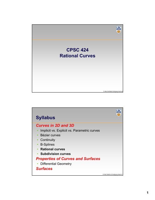
<strong>CPSC</strong> <strong>424</strong><br />
<strong>Rational</strong> <strong>Curves</strong><br />
© Alla Sheffer& Wolfgang Heidrich<br />
<strong>Syllabus</strong><br />
<strong>Curves</strong> in 2D and 3D<br />
• Implicit vs. Explicit vs. Parametric curves<br />
• Bézier curves<br />
• Continuity<br />
• B-Splines<br />
• <strong>Rational</strong> curves<br />
• Subdivision curves<br />
Properties of <strong>Curves</strong> and Surfaces<br />
• Differential Geometry<br />
Surfaces<br />
© Alla Sheffer & Wolfgang Heidrich<br />
1
<strong>Rational</strong> <strong>Curves</strong><br />
Motivation<br />
• Conic sections:<br />
– All curves generated by the intersection of a cone<br />
with a plane<br />
– Parabolae, hyperbolae, ellipses/circles<br />
• Bézier and B-Spline curves <strong>ca</strong>nnot represent all conic<br />
sections<br />
– Parabolae possible, but not hyperbolae and<br />
ellipses/circles<br />
– We have seen a hint of this in assignment 2 for the<br />
example of circles…<br />
© Alla Sheffer & Wolfgang Heidrich<br />
<strong>Rational</strong> <strong>Curves</strong><br />
Motivation (cont)<br />
• Bézier and B-Spline curves are invariant under affine<br />
transformations but not projective transformations<br />
• Example: <strong>ca</strong>noni<strong>ca</strong>l perspective transformation<br />
Fx<br />
( t) / Fz<br />
( t)<br />
Fx<br />
( t)<br />
<br />
<br />
<br />
Fy<br />
( t) / Fz<br />
( t)<br />
<br />
Fy<br />
( t)<br />
<br />
1/ F ( t)<br />
1 <br />
z<br />
<br />
1 Fz<br />
( t)<br />
<br />
1<br />
Fx<br />
( t)<br />
<br />
<br />
<br />
Fy<br />
( t)<br />
<br />
1<br />
F<br />
( t)<br />
<br />
z<br />
<br />
1 <br />
division on right side <strong>ca</strong>nnot be represented with the<br />
de Casteljau or de Boor algorithm<br />
<br />
<br />
<br />
<br />
<br />
1<br />
1<br />
© Alla Sheffer & Wolfgang Heidrich<br />
2
<strong>Rational</strong> <strong>Curves</strong><br />
Definition:<br />
• A rational curve is of the form<br />
F(<br />
t) : <br />
m<br />
<br />
i0<br />
m<br />
B<br />
<br />
i0<br />
m<br />
i<br />
B<br />
( t)<br />
w<br />
m<br />
i<br />
i<br />
( t)<br />
w<br />
b<br />
i<br />
i<br />
<br />
B<br />
m m<br />
i<br />
m<br />
i0<br />
<br />
m<br />
B<br />
j<br />
j0<br />
( t)<br />
w<br />
i<br />
( t)<br />
w<br />
j<br />
b<br />
i<br />
w<br />
0,<br />
w0 w 1<br />
with weights<br />
Note:<br />
i<br />
m<br />
• We <strong>ca</strong>n use either of Bézier and B-Spline basis here<br />
© Alla Sheffer & Wolfgang Heidrich<br />
<strong>Rational</strong> <strong>Curves</strong><br />
In homogeneous coordinates:<br />
• Note that we get the original Bezier<br />
curves if all weights are 1!<br />
• Clear from this representation:<br />
the projective image of a rational<br />
curve is again a rational curve<br />
(projective invariance)<br />
<br />
<br />
<br />
<br />
<br />
F(<br />
t) : <br />
<br />
<br />
<br />
<br />
<br />
m<br />
<br />
i0<br />
m<br />
<br />
i0<br />
m<br />
<br />
i0<br />
m<br />
B<br />
B<br />
B<br />
<br />
i0<br />
m<br />
i<br />
m<br />
i<br />
m<br />
i<br />
B<br />
( t)<br />
w<br />
( t)<br />
w<br />
( t)<br />
w<br />
m<br />
i<br />
i<br />
i<br />
i<br />
z<br />
( t)<br />
w<br />
x<br />
y<br />
i<br />
<br />
<br />
<br />
<br />
<br />
<br />
<br />
<br />
<br />
<br />
<br />
i<br />
i<br />
i<br />
© Alla Sheffer & Wolfgang Heidrich<br />
3
<strong>Rational</strong> <strong>Curves</strong><br />
Other properties:<br />
• Convex hull<br />
• Curve interpolates start and endpoint (rational Bézier<br />
only)<br />
• De Casteljau, de Boor and other algorithms now have<br />
to be performed in homogeneous coordinates!<br />
© Alla Sheffer & Wolfgang Heidrich<br />
OpenGL<br />
void gluNurbsCurve( GLUnurbsObj *nobj, GLint nknots,<br />
GLfloat *knot, GLint stride, GLfloat *ctlarray, GLint order,<br />
GLenum type )<br />
nobj - pointer to object created by gluNewNurbsRenderer<br />
nknots - number of knots<br />
knot – knot vector<br />
stride - “width” = dimension<br />
ctlarray - array of control points.<br />
order - degree+1<br />
type - enum of types<br />
© Alla Sheffer & Wolfgang Heidrich<br />
4
OpenGL - example<br />
GLfloat knots[8] = {<br />
0.0, 0.0, 0.0, 0.0, 1.0, 1.0, 1.0, 1.0<br />
};<br />
gluBeginCurve(nurb);<br />
gluNurbsCurve(nurb, 8, knots, 3, &ctlpoints[0][0],<br />
4, GL_MAP1_VERTEX_3);<br />
gluEndCurve(nurb);<br />
© Alla Sheffer & Wolfgang Heidrich<br />
Subdivision <strong>Curves</strong><br />
Represent smooth curve by approximating<br />
polyline<br />
At the limit = curve<br />
Each iteration<br />
• Add new points (~double)<br />
• Approximating - Move old points<br />
• Interpolating – Keep old points<br />
© Alla Sheffer & Wolfgang Heidrich<br />
5
Bezier Subdivision<br />
To create complex curve need to explicitly<br />
enforce continuity – not very useful<br />
© Alla Sheffer & Wolfgang Heidrich<br />
Corner Cutting<br />
© Alla Sheffer & Wolfgang Heidrich<br />
6
Corner Cutting<br />
© Alla Sheffer & Wolfgang Heidrich<br />
Corner Cutting<br />
© Alla Sheffer & Wolfgang Heidrich<br />
7
Corner Cutting<br />
© Alla Sheffer & Wolfgang Heidrich<br />
Corner Cutting<br />
© Alla Sheffer & Wolfgang Heidrich<br />
8
Corner Cutting<br />
© Alla Sheffer & Wolfgang Heidrich<br />
Corner Cutting<br />
© Alla Sheffer & Wolfgang Heidrich<br />
9
Corner Cutting<br />
© Alla Sheffer & Wolfgang Heidrich<br />
Corner Cutting – Chaikin Algorithm<br />
control point<br />
limit curve<br />
control polygon<br />
Limit – quadratic B-spline curve<br />
© Alla Sheffer & Wolfgang Heidrich<br />
10
Cubic B-Spline (corner cutting)<br />
3/4<br />
1/8 1/8<br />
© Alla Sheffer & Wolfgang Heidrich<br />
Cubic Corner Cutting<br />
© Alla Sheffer & Wolfgang Heidrich<br />
11
The 4-point scheme<br />
© Alla Sheffer & Wolfgang Heidrich<br />
The 4-point scheme<br />
© Alla Sheffer & Wolfgang Heidrich<br />
12
The 4-point scheme<br />
© Alla Sheffer & Wolfgang Heidrich<br />
The 4-point scheme<br />
© Alla Sheffer & Wolfgang Heidrich<br />
13
The 4-point scheme<br />
© Alla Sheffer & Wolfgang Heidrich<br />
The 4-point scheme<br />
© Alla Sheffer & Wolfgang Heidrich<br />
14
The 4-point scheme<br />
© Alla Sheffer & Wolfgang Heidrich<br />
The 4-point scheme<br />
© Alla Sheffer & Wolfgang Heidrich<br />
15
The 4-point scheme<br />
© Alla Sheffer & Wolfgang Heidrich<br />
The 4-point scheme<br />
© Alla Sheffer & Wolfgang Heidrich<br />
16
The 4-point scheme<br />
© Alla Sheffer & Wolfgang Heidrich<br />
The 4-point scheme<br />
© Alla Sheffer & Wolfgang Heidrich<br />
17
The 4-point scheme<br />
© Alla Sheffer & Wolfgang Heidrich<br />
The 4-point scheme<br />
© Alla Sheffer & Wolfgang Heidrich<br />
18
The 4-point scheme<br />
© Alla Sheffer & Wolfgang Heidrich<br />
The 4-point scheme<br />
control point<br />
limit curve<br />
control polygon<br />
© Alla Sheffer & Wolfgang Heidrich<br />
19
Subdivision curves<br />
Non interpolatory subdivision schemes<br />
• Corner Cutting<br />
Interpolatory subdivision schemes<br />
• The 4-point scheme<br />
© Alla Sheffer & Wolfgang Heidrich<br />
20