Mapping Electric and Potential Fields
Mapping Electric and Potential Fields
Mapping Electric and Potential Fields

You also want an ePaper? Increase the reach of your titles
YUMPU automatically turns print PDFs into web optimized ePapers that Google loves.
<strong>Mapping</strong> <strong>Electric</strong> <strong>and</strong> <strong>Potential</strong> <strong>Fields</strong><br />
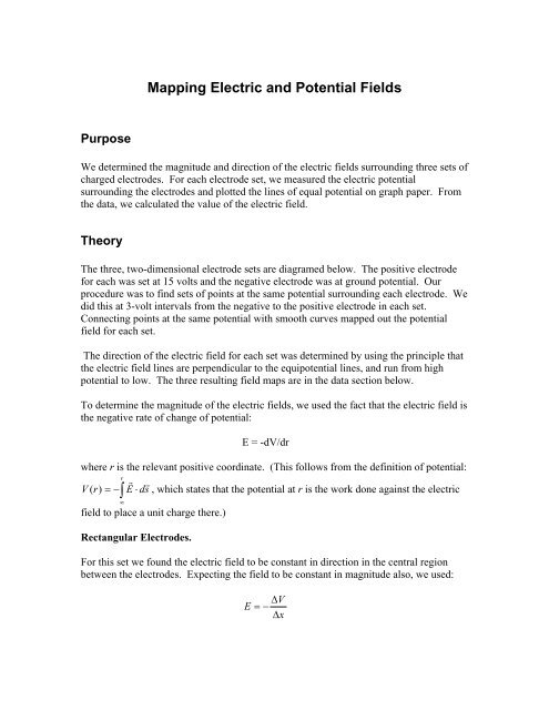
Purpose<br />
We determined the magnitude <strong>and</strong> direction of the electric fields surrounding three sets of<br />
charged electrodes. For each electrode set, we measured the electric potential<br />
surrounding the electrodes <strong>and</strong> plotted the lines of equal potential on graph paper. From<br />
the data, we calculated the value of the electric field.<br />
Theory<br />
The three, two-dimensional electrode sets are diagramed below. The positive electrode<br />
for each was set at 15 volts <strong>and</strong> the negative electrode was at ground potential. Our<br />
procedure was to find sets of points at the same potential surrounding each electrode. We<br />
did this at 3-volt intervals from the negative to the positive electrode in each set.<br />
Connecting points at the same potential with smooth curves mapped out the potential<br />
field for each set.<br />
The direction of the electric field for each set was determined by using the principle that<br />
the electric field lines are perpendicular to the equipotential lines, <strong>and</strong> run from high<br />
potential to low. The three resulting field maps are in the data section below.<br />
To determine the magnitude of the electric fields, we used the fact that the electric field is<br />
the negative rate of change of potential:<br />
E = -dV/dr<br />
where r is the relevant positive coordinate. (This follows from the definition of potential:<br />
r<br />
<br />
V ( r)<br />
= − E ⋅ ds , which states that the potential at r is the work done against the electric<br />
∫<br />
∞<br />
field to place a unit charge there.)<br />
Rectangular Electrodes.<br />
For this set we found the electric field to be constant in direction in the central region<br />
between the electrodes. Expecting the field to be constant in magnitude also, we used:<br />
ΔV<br />
E = −<br />
Δx
to determine the average value of the field in this region. The position coordinate x was<br />
measured from the negative electrode.<br />
Concentric Electrodes<br />
In this case we found the equipotentials to be roughly circular, indicating a radially<br />
directed electric field. Since the distance between field lines increases (<strong>and</strong> the<br />
magnitude of the field thus decreases) in proportion to the radial distance r, the electric<br />
field for such a two-dimensional configuration must have the form<br />
V<br />
E =<br />
r<br />
m<br />
where V m is some constant voltage. In turn, this means the potential must have the form:<br />
V ( r)<br />
= V<br />
a<br />
−<br />
V<br />
m<br />
r<br />
ln( )<br />
a<br />
where a is the radius of the inner electrode <strong>and</strong> V a is the potential there. (This can be<br />
dV Vm<br />
derived from E = − = <strong>and</strong> integrating from r=a to arbitrary radius r.)<br />
dr r<br />
We measured the average radii of the equipotential lines <strong>and</strong> plotted ln(r/a) versus the<br />
potential V. From the slope of this graph, we determined V m . Using this, we calculated<br />
the magnitude of the electric field at the radii of the equipotentials.<br />
Circular Electrodes.<br />
The potential lines here were ovoid, indicating a field that depends on both position<br />
coordinates: x <strong>and</strong> y (or r <strong>and</strong> θ). We confined ourselves to calculating the field along<br />
the central axis only using<br />
ΔV<br />
E(<br />
x)<br />
≈ −<br />
Δx<br />
where the position coordinate x was measured from the positive electrode. We expect<br />
this to be an approximation to the field values half way between each equipotential line.
Experiment Set up<br />
The electrodes consisted of two-dimensional regions drawn with metallic ink on<br />
conductive paper:<br />
Set 1 (rectangular) Two rectangles 12 cm x 1 cm, 9 cm apart<br />
Set 2 (concentric) Positive electrode: a circle of radius 1 cm<br />
Negative electrode: a circle of radius 8 cm<br />
Set 3 (circles)<br />
Two circles of radius 1 cm, centers 10 cm apart.<br />
A 15-volt potential difference was applied across the electrodes with a low-voltage power<br />
supply.<br />
We measured the potential using a VC 9808 Digital Multimeter. The meter was<br />
connected to the negative electrode <strong>and</strong> a voltage probe was touched to the paper to test<br />
the voltage at the point of interest.<br />
For each set, we found the 3-volt, 6-volt, 9-volt <strong>and</strong> 12-volt equipotential lines.<br />
Rectangular Concentric Circular<br />
Data<br />
(See diagrams below.)
Analysis<br />
The field maps can be seen below. The electric field calculations are as follows.<br />
Rectangular electrodes<br />
We measured the positions of the equipotentials along the central line between the<br />
electrodes. The position (x) was measured from the positive electrode. From this, we<br />
calculated average value of the field. The results are<br />
<strong>Potential</strong> (V) Position (cm) E-field (V/cm) deviation (V/cm)<br />
15.0 0.0<br />
12.0 1.9 1.6 -.1<br />
9.0 3.6 1.8 .1<br />
6.0 5.4 1.7 0<br />
3.0 7.3 1.6 -.1<br />
0.0 9.0 1.8 .1<br />
Average: 1.7 .1 (σ = .1)<br />
E-Field value: 1 .7 ± . 1 volts/cm, or<br />
170 ± 10 volts/meter<br />
Results have been rounded to 2 significant figures.<br />
Concentric Electrodes<br />
The average values for the equipotential radii are listed in the table below. Also below is<br />
a semi-log plot of (r/a) versus the potential.<br />
The slope of the graph, using the indicated values on the plot, is<br />
Slope =<br />
ln( 1.95/ 6.8)<br />
10.25 −1.25<br />
= −.139volts<br />
−1<br />
The y-intercept is ln(8). The equation of the graph is<br />
ln(r/a) = ln(8) - .139 V(r)<br />
r<br />
Comparing this with V ( r)<br />
= V − a<br />
Vm<br />
ln( ) , we have<br />
a
V m = 1/.139 = 7.19 volts<br />
Using V(r=8cm) = 0 volts, V a = 15 volts <strong>and</strong> r = 8 cm, <strong>and</strong> plugging into the theoretical<br />
expression for V(r), we get<br />
V m = 7.21 volts<br />
(theory)<br />
Our empirical results differ from theory by 0.2%.<br />
The values of the electric field at the radii of the equipotentials were calculated using our<br />
empirical value for V m. The results are below.<br />
V(volts) r (cm) E (volts/cm)<br />
15.0 1.0 7.2<br />
12.0 1.6 4.5<br />
9.0 2.4 3.0<br />
6.0 3.7 1.9<br />
3.0 5.3 1.4<br />
0.0 8.0 0.9<br />
(rounded to 2 significant figures)<br />
Circular Electrodes<br />
We determined the positions of the equipotentials on the central line between the<br />
electrodes. We approximated the electric field strength at the midpoints between<br />
equipotentials by calculating the average value of the field between them (ΔV/Δx).<br />
x (cm) V(x)(volts) midpoint (cm) <strong>Electric</strong> Field (V/cm)<br />
1.0 15.0<br />
2.2 12.0<br />
4.1 9.0<br />
6.2 6.0<br />
8.0 3.0<br />
9.1 0.0<br />
1.6 2.5<br />
3.2 1.6<br />
5.2 1.4<br />
7.1 1.7<br />
8.6 2.7
Conclusions<br />
The electric field between rectangular electrodes is roughly constant in magnitude <strong>and</strong><br />
direction in the region away from the ends of the electrodes. The field bulges out at the<br />
end of the electrodes. For very long rectangles, we would expect the field to be very<br />
uniform in the central region. We would expect this also to apply to rectangular plates or<br />
parallel sheets of any shape: uniform in the center, with bulging at the edges.<br />
The concentric configuration led to radial fields, with the potential varying<br />
logarithmically <strong>and</strong> the electric field going as 1/r. The field was zero outside the outer<br />
electrode. The same should be true for cylindrical electrodes, as in coaxial cables.<br />
The circular electrodes led to ovoid potential lines. The field was strongest near each<br />
electrode, weaker in the central region between them, <strong>and</strong> weakest far from the electrodes<br />
(since the field lines become sparse there). We would expect any two localized regions<br />
of opposite charge, separated by a small distance, to have a similar field. (Such a field is<br />
called a dipole field.) For instance, a water molecule is known to have this type of charge<br />
separation, <strong>and</strong> many of the properties of water are due to the dipole field surrounding its<br />
molecules.