Linear response and Time dependent Hartree-Fock

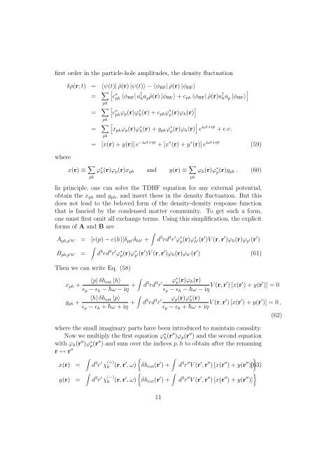
first order in the particle-hole amplitudes, the density fluctuation
δρ(r; t) = 〈ψ(t)| ˆρ(r) |ψ(t)〉 − 〈φ HF | ˆρ(r) |φ HF 〉
[
c
∗
ph 〈φ HF | a † h a p ˆρ(r) |φ HF 〉 + c ph 〈φ HF | ˆρ(r)a † h a p |φ HF 〉 ]
= ∑ ph
= ∑ ph
[
c
∗
ph ϕ p (r)ϕ ∗ h(r) + c ph ϕ ∗ p(r)ϕ h (r) ]
= ∑ ph
[
xph ϕ p (r)ϕ ∗ h(r) + y ph ϕ ∗ p(r)ϕ h (r) ] e iωt+ηt + c.c.
where
= [x(r) + y(r)] e −iωt+ηt + [x ∗ (r) + y ∗ (r)] e iωt+ηt (59)
x(r) ≡ ∑ ph
ϕ ∗ h(r)ϕ p (r)x ph and y(r) ≡ ∑ ph
ϕ h (r)ϕ ∗ p(r)y ph . (60)
In principle, one can solve the TDHF equation for any external potential,
obtain the x ph and y ph , and insert these in the density fluctuation. But this
does not lead to the beloved form of the density-density response function
that is fancied by the condensed matter community. To get such a form,
one must first omit all exchange terms. Using this simplification, the explicit
forms of A and B are
∫
A ph,p ′ h ′ = [e(p) − e(h)]δ pp ′δ hh ′ + d 3 rd 3 r ′ ϕ ∗ p(r)ϕ ∗ h ′(r′ )V (r, r ′ )ϕ h (r)ϕ p ′(r ′ )
∫
B ph,p ′ h ′ = d 3 rd 3 r ′ ϕ ∗ p(r)ϕ ∗ p ′(r′ )V (r, r ′ )ϕ h (r)ϕ h ′(r ′ ) (61)
Then we can write Eq. (58)
x ph +
y ph +
∫
〈p| δh ext |h〉
ɛ p − ɛ h − ¯hω − iη + ∫
〈h| δh ext |p〉
ɛ p − ɛ h + ¯hω + iη +
d 3 rd 3 r ′ ϕ ∗ p(r)ϕ h (r)
ɛ p − ɛ h − ¯hω − iη V (r, r′ ) [x(r ′ ) + y(r ′ )] = 0
d 3 rd 3 r ′ ϕ p (r)ϕ ∗ h(r)
ɛ p − ɛ h + ¯hω + iη V (r, r′ ) [x(r ′ ) + y(r ′ )] = 0 ,
where the small imaginary parts have been introduced to maintain causality.
Now we multiply the first equation ϕ ∗ h(r ′′ )ϕ p (r ′′ ) and the second equation
with ϕ h (r ′′ )ϕ ∗ p(r ′′ ) and sum over the indices p, h to obtain after the renaming
r ↔ r ′′
x(r) =
y(r) =
∫
∫
d 3 r ′ χ (+)
{
0 (r, r ′ , ω)
d 3 r ′ χ (−)
0 (r, r ′ , ω)
∫
δh ext (r ′ ) +
{
∫
δh ext (r ′ ) +
11
}
d 3 r ′′ V (r ′ , r ′′ ) [x(r ′′ ) + y(r ′′ )] (63)
}
d 3 r ′′ V (r ′ , r ′′ ) [x(r ′′ ) + y(r ′′ )]
(62)