Comparison of methods for solving the Schrödinger equation for ...
Comparison of methods for solving the Schrödinger equation for ...
Comparison of methods for solving the Schrödinger equation for ...

You also want an ePaper? Increase the reach of your titles
YUMPU automatically turns print PDFs into web optimized ePapers that Google loves.
Proc. Estonian Acad. Sci. Eng., 2006, 12, 3-2, 246–261<br />
a<br />
b<br />
<strong>Comparison</strong> <strong>of</strong> <strong>methods</strong> <strong>for</strong> <strong>solving</strong><br />
<strong>the</strong> Schrödinger <strong>equation</strong> <strong>for</strong> multiquantum<br />
well heterostructure applications<br />
Andres Udal a , Reeno Reeder a , Enn Velmre a and Paul Harrison b<br />
Department <strong>of</strong> Electronics, Tallinn University <strong>of</strong> Technology, Ehitajate tee 5, 19086 Tallinn,<br />
Estonia; audal@va.ttu.ee, reeno@cyber.ee, evelmre@ttu.ee<br />
School <strong>of</strong> Electronic and Electrical Engineering, University <strong>of</strong> Leeds, LS2 9JT, United Kingdom,<br />
p.harrison@leeds.ac.uk<br />
Received 23 May 2006, in revised <strong>for</strong>m 7 July 2006<br />
Abstract. Direct numerical approaches <strong>for</strong> <strong>the</strong> solution <strong>of</strong> <strong>the</strong> time-independent one-dimensional<br />
Schrödinger <strong>equation</strong> are discussed. Applications to multiquantum well (MQW) semiconductor<br />
heterostructure potentials need linear dependence <strong>of</strong> <strong>the</strong> computer time t comp<br />
on <strong>the</strong> number <strong>of</strong><br />
spatial grid points N . Although acknowledged as a very effective Fourier grid Hamiltonian (FGH)<br />
3<br />
method, it has cubic dependence on <strong>the</strong> number <strong>of</strong> spatial grid points, i.e., t ∼ N , which limits<br />
comp<br />
its use to problems with a complexity <strong>of</strong> N ≤ 1000. A simple straight<strong>for</strong>ward shooting method<br />
(ShM), which is based on trial stepping over <strong>the</strong> coordinate and energy, has <strong>the</strong> necessary t comp<br />
∼ N<br />
dependence with moderate energy convergence efficiency but <strong>the</strong> recommended symmetry preconditions<br />
and <strong>the</strong> not very clearly defined external boundaries make its application inconvenient.<br />
This paper <strong>of</strong>fers a new reliable and effective energy and wave function coupled solution (EWC)<br />
method with a Newton iteration scheme and an internal bordered tridiagonal matrix solver. The<br />
method has a linear t comp<br />
∼ N dependence and may by applied to arbitrary potential energy<br />
5<br />
distribution tasks with complexity up to N = 10 and beyond. Zero or cyclic boundary conditions<br />
may be specified <strong>for</strong> <strong>the</strong> wave function. For versatile MQW tasks <strong>the</strong> combined use <strong>of</strong> ShM and<br />
EWC is illustrated. Detailed accuracy and computer time comparisons show that <strong>the</strong> combined<br />
ShM + EWC method is three orders <strong>of</strong> magnitude more effective than <strong>the</strong> FGH method.<br />
Key words: multiquantum well structures, Schrödinger <strong>equation</strong>, bound states, numerical <strong>methods</strong>,<br />
energy, wave function.<br />
1. INTRODUCTION<br />
In spite <strong>of</strong> <strong>the</strong> fact that Erwin Schrödinger <strong>for</strong>mulated his famous <strong>equation</strong> 80<br />
years ago in 1926 and that <strong>for</strong> over 70 years scientists have proposed various<br />
analytical and numerical <strong>methods</strong> <strong>for</strong> <strong>the</strong> solution <strong>of</strong> this central quantum<br />
246
mechanics <strong>equation</strong>, approaches even to one-dimensional solutions are still a<br />
subject <strong>of</strong> debate. This is confirmed by <strong>the</strong> continuing appearance <strong>of</strong> new<br />
publications in this field [ 1–6 ]. Since 1990s, one <strong>of</strong> <strong>the</strong> driving <strong>for</strong>ces in this field<br />
has been physical chemistry and its applications. The second spur <strong>of</strong> motivation<br />
has come from <strong>the</strong> extremely wide application area in semiconductor heterostructures<br />
with quantum wells, wires and dots [ 7 ]. Although nowadays <strong>the</strong><br />
available sophisticated ab-initio s<strong>of</strong>tware tools already make quite realistic threedimensional<br />
calculations possible, almost every research task needs an estimation<br />
<strong>of</strong> static bound states in a one-dimensional (1D) approximation ei<strong>the</strong>r in spherical<br />
or rectangular coordinates. The last case is more typical <strong>for</strong> semiconductor<br />
heterostructures where <strong>the</strong> calculation <strong>of</strong> 1D bound states <strong>for</strong> complex multibarrier<br />
quantum well systems like, e.g. in quantum cascade lasers [ 8 ] or digitized<br />
quasi-parabolic quantum wells [ 9 ], may be a ra<strong>the</strong>r time-consuming subtask.<br />
In applications in physical chemistry, <strong>the</strong> potentials in <strong>the</strong> atomic subnanometer<br />
scale are ra<strong>the</strong>r smooth and relatively small number ( N ≤ 100) <strong>of</strong> spatial<br />
grid points may be sufficient to obtain accurate results. In contrast to that, MQW<br />
structures with great numbers <strong>of</strong> relatively abrupt potential steps over <strong>the</strong> 10–<br />
4<br />
1000 nm spatial scale may need spatial grid sizes over N > 10 to achieve<br />
acceptable results [ 7,9 ]. This means that <strong>for</strong> <strong>the</strong> analysis and even more <strong>for</strong> <strong>the</strong><br />
optimization <strong>of</strong> MQW structures <strong>the</strong> <strong>methods</strong> <strong>of</strong> <strong>solving</strong> <strong>the</strong> Schrödinger<br />
<strong>equation</strong> must consume computer time no more than proportionally to N .<br />
The FGH method [ 1–3 ] has been declared to be very effective and <strong>the</strong> simplest<br />
method <strong>for</strong> <strong>the</strong> calculation <strong>of</strong> bound states from <strong>the</strong> time-independent 1D<br />
Schrödinger <strong>equation</strong>. It can take as input an arbitrary potential distribution, but<br />
its computer execution time t comp scales as N 3 . The use <strong>of</strong> <strong>the</strong> Fast Fourier<br />
Trans<strong>for</strong>m in <strong>the</strong> construction <strong>of</strong> <strong>the</strong> Hamiltonian matrix may reduce <strong>the</strong> last<br />
2<br />
number to N × ln N but not more [ 2 ]. The internal algebraic solver <strong>of</strong> <strong>the</strong> FGH<br />
method uses standard procedures from <strong>the</strong> EISPACK computer package [ 10 ].<br />
Actually, <strong>the</strong> most elementary solution method with <strong>the</strong> required linear<br />
dependence <strong>of</strong> <strong>the</strong> computer time on <strong>the</strong> grid size ( t comp<br />
∼ N)<br />
is <strong>the</strong> shooting<br />
method [ 7 ], which finds eigenvalues <strong>of</strong> <strong>the</strong> bound state energy by using a trial<br />
procedure, based on <strong>the</strong> condition that an iteration over <strong>the</strong> spatial coordinate<br />
from <strong>the</strong> centre <strong>of</strong> <strong>the</strong> active area into <strong>the</strong> surrounding barriers must yield a<br />
vanishing wave function Ψ → 0. The ShM needs two initial values <strong>of</strong> <strong>the</strong> wave<br />
function to start <strong>the</strong> iteration over <strong>the</strong> spatial coordinate. Those two values may<br />
be correctly defined <strong>for</strong> symmetric potentials but in <strong>the</strong> general case it needs an<br />
approximate auxiliary algorithm [ 7 ]. Ano<strong>the</strong>r problem, troubling <strong>the</strong> application<br />
<strong>of</strong> <strong>the</strong> ShM, is associated with <strong>the</strong> exponentially growing components <strong>of</strong> <strong>the</strong><br />
wave function in <strong>the</strong> outer barrier regions, which can impede <strong>the</strong> detection <strong>of</strong> <strong>the</strong><br />
<strong>the</strong>oretical boundary condition Ψ → 0.<br />
In <strong>the</strong> present work we propose an effective iterative coupled energy and wave<br />
function method <strong>for</strong> <strong>solving</strong> <strong>the</strong> time-independent one-dimensional Schrödinger<br />
<strong>equation</strong>, which possesses linear t comp<br />
∼ N dependence and may be applied to<br />
arbitrary potential energy distributions without any symmetry restrictions. The<br />
247
method uses an iterative approach in <strong>the</strong> Newton method and its internal algebraic<br />
task involves <strong>the</strong> solution <strong>of</strong> a linear system, represented by a bordered tri-diagonal<br />
matrix; zero or cyclic boundary conditions may be specified. In <strong>the</strong> case <strong>of</strong><br />
arbitrarily complex MQW problems <strong>the</strong> combined ShM + EWC approach is<br />
necessary when approximate wave functions and estimations <strong>for</strong> <strong>the</strong> energy<br />
eigenvalues <strong>for</strong> <strong>the</strong> EWC method are supplied by <strong>the</strong> ShM. Considering <strong>for</strong>mation<br />
<strong>of</strong> <strong>the</strong> Jacobi matrix in <strong>the</strong> Newton method by zero boundary conditions, <strong>the</strong> EWC<br />
method is similar to <strong>the</strong> known relaxational approach [ 4 ]. As one can see below,<br />
direct comparison <strong>of</strong> FGH and ShM + EWC <strong>methods</strong> reveals that <strong>the</strong> latter may be<br />
over three orders <strong>of</strong> magnitudes more effective than <strong>the</strong> FGH method <strong>for</strong> tasks with<br />
N > 1000. Some results <strong>of</strong> application <strong>of</strong> <strong>the</strong> present work are published in [ 9 ].<br />
In <strong>the</strong> present study we discuss nei<strong>the</strong>r semi-analytical approaches with specific<br />
application areas like [ 6 ] nor <strong>the</strong> new original “random trial” approaches [ 5 ].<br />
248<br />
2. METHODS OF THE NUMERICAL SOLUTION<br />
2.1. The Fourier grid Hamiltonian method<br />
The Fourier grid Hamiltonian method <strong>for</strong> numerical solution <strong>of</strong> <strong>the</strong> timeindependent<br />
Schrödinger <strong>equation</strong> was introduced in 1989 by Marston and Balint-<br />
Kurti [ 1 ]. Initially it was <strong>for</strong>mulated <strong>for</strong> an odd number <strong>of</strong> coordinate grid points N<br />
in rectangular coordinates [ 1 ]. Later it was modified <strong>for</strong> an even number <strong>of</strong> grid<br />
points and <strong>for</strong> spherical coordinates with <strong>the</strong> possibility <strong>of</strong> applying <strong>the</strong> Fast<br />
Fourier Trans<strong>for</strong>m to accelerate <strong>the</strong> <strong>for</strong>mation <strong>of</strong> <strong>the</strong> Hamiltonian matrix [ 2,3 ]. The<br />
<strong>the</strong>ory behind <strong>the</strong> method is based on relating <strong>the</strong> potential energy at <strong>the</strong> N grid<br />
points with <strong>the</strong> kinetic energy in <strong>the</strong> momentum space via <strong>for</strong>ward and reverse<br />
Fourier trans<strong>for</strong>ms between <strong>the</strong> coordinate and <strong>the</strong> momentum space. The N×<br />
N<br />
symmetric matrix H , obtained by discretization, has elements in <strong>the</strong> <strong>for</strong>m <strong>of</strong><br />
cosine sums. The task <strong>of</strong> calculating <strong>the</strong> bound state eigenenergies and eigenfunctions<br />
is <strong>the</strong>reby trans<strong>for</strong>med to <strong>the</strong> task <strong>of</strong> finding eigenvalues and eigenvectors<br />
<strong>of</strong> <strong>the</strong> matrix H . As suggested by <strong>the</strong> authors <strong>of</strong> <strong>the</strong> FGH method, this may<br />
be accomplished by standard subroutines such as <strong>the</strong> EISPACK package [ 10 ]. The<br />
source code <strong>of</strong> <strong>the</strong> computer implementation <strong>of</strong> <strong>the</strong> method, FGHEVEN [ 2 ], <strong>for</strong> an<br />
even number <strong>of</strong> nodes, is freely distributed via <strong>the</strong> internet [ 11 ]. Subsequently, <strong>the</strong><br />
method was extended to <strong>the</strong> three-dimensional case [ 12 ]. In <strong>the</strong> present work we<br />
have realized <strong>the</strong> odd number FGH method in rectangular coordinates and in <strong>the</strong> SI<br />
unit system <strong>for</strong> testing, following reference [ 1 ].<br />
Assuming that <strong>the</strong> length <strong>of</strong> <strong>the</strong> calculation area L is divided into N steps,<br />
<strong>the</strong> discrete grid is defined as<br />
x = ( i−1 2) ∆x, ∆ x= L N, i= 1, 2, ..., N.<br />
(1)<br />
i<br />
Equation (1), which defines nodes in <strong>the</strong> centre <strong>of</strong> every interval ∆ x,<br />
differs<br />
somewhat from <strong>the</strong> original one x i<br />
= i∆ x [ 1 ] but is more correct in <strong>the</strong> case <strong>of</strong><br />
symmetric QW tasks.
Following [ 1 ], <strong>the</strong> spatial discretization and trans<strong>for</strong>mations per<strong>for</strong>med yield a<br />
symmetric matrix H <strong>of</strong> size N×<br />
N<br />
n<br />
2<br />
Hij = ∑cos( l2 π( i− j) N) Tl + V( xi ) δij, n= ( N −1) 2,<br />
N l=<br />
1<br />
(2)<br />
2<br />
2 ⎛ ⎞ π l ħ<br />
Tl<br />
⎟ ⎜ = ,<br />
⎠ ⎝ m L<br />
where ≡ h ħ 2π<br />
is <strong>the</strong> reduced Planck constant, m is <strong>the</strong> electron rest mass and<br />
<strong>the</strong> Kronecker symbol δ ij ensures that potential energy values at grid nodes<br />
V ( x i<br />
) are only added to <strong>the</strong> main diagonal.<br />
The EISPACK subroutines return N eigenvalues and N eigenfunctions with<br />
values at all N grid nodes. The eigenvalues, which lie below <strong>the</strong> potential energy<br />
values at <strong>the</strong> solution area borders V (0) and V ( L ), may be interpreted as <strong>the</strong><br />
bound state energies <strong>of</strong> <strong>the</strong> system [ 1 ]. The o<strong>the</strong>r eigenvalues may be interpreted<br />
as extraneous solutions, which un<strong>for</strong>tunately consume computer time <strong>for</strong> <strong>the</strong>ir<br />
calculation. On <strong>the</strong> o<strong>the</strong>r hand, <strong>the</strong> maximum number <strong>of</strong> eigenvalues is limited by<br />
<strong>the</strong> grid size N . As experience shows, in practical quantum well calculations<br />
sufficiently thick outer barrier layers with a sufficiently high potential V must be<br />
included to ensure sufficient decay <strong>of</strong> wave functions and hence remove any<br />
uncertainty in <strong>the</strong> boundary conditions in <strong>the</strong> FGH method. It should be added<br />
that by selecting different subroutines from <strong>the</strong> EISPACK package, it is possible<br />
to calculate <strong>the</strong> energies without wave functions [ 11 ], which reduces <strong>the</strong> computation<br />
time approximately 1.5 times.<br />
2.2. The shooting method<br />
The shooting method is one <strong>of</strong> <strong>the</strong> simplest numerical algorithms and its key<br />
idea is to replace a boundary condition problem with multiple trial runs <strong>of</strong> a<br />
remarkably simple initial condition task. This is also <strong>the</strong> most straight<strong>for</strong>ward<br />
method <strong>for</strong> solution <strong>of</strong> <strong>the</strong> time-independent Schrödinger <strong>equation</strong> if <strong>the</strong> varied<br />
trial parameter is <strong>the</strong> energy E ([ 7 ], Chapter 3). The trial energy equals <strong>the</strong><br />
bound state energy if <strong>the</strong> wave function vanishes ( Ψ → 0) in <strong>the</strong> surrounding<br />
barriers when moving away from <strong>the</strong> QW area. In spite <strong>of</strong> <strong>the</strong> extreme simplicity,<br />
ShM has a linear dependence <strong>of</strong> <strong>the</strong> computer time on <strong>the</strong> grid node number<br />
tcomp ∼ N,<br />
which makes it efficient <strong>for</strong> MQW tasks.<br />
The time-independent 1D Schrödinger <strong>equation</strong> in its classical <strong>for</strong>m, where<br />
kinetic energy is defined by <strong>the</strong> second spatial derivative, reads<br />
2 2<br />
∂ Ψ<br />
VΨ<br />
EΨ.<br />
2<br />
ħ<br />
− + =<br />
2m<br />
∂x<br />
In <strong>the</strong> present study, which is focused on <strong>the</strong> effectiveness <strong>of</strong> numerical<br />
<strong>methods</strong>, we ignore <strong>the</strong> fact that in semiconductor heterostructures, a more<br />
sophisticated kinetic energy term [ 7 ]<br />
(3)<br />
249
2<br />
∂ 1 ∂Ψ<br />
ħ<br />
−<br />
2 ∂ m ∂x<br />
is recommended <strong>for</strong> tasks with a variable effective mass m( x ).<br />
To realize discrete stepping over <strong>the</strong> spatial coordinate, <strong>the</strong> second derivative<br />
in <strong>the</strong> Schrödinger <strong>equation</strong> (3) is replaced by a three-point discretization scheme<br />
2<br />
Ψi+ 1−Ψi Ψi −Ψi−<br />
⎛<br />
1⎞<br />
1<br />
ħ<br />
− − + ViΨ<br />
⎜<br />
⎟<br />
i = EΨi,<br />
⎠<br />
⎝ 2m ∆x ∆x ∆x<br />
where Ψ<br />
i<br />
denotes Ψ ( x i<br />
) and Vi<br />
≡ V( xi<br />
).<br />
To initialize <strong>the</strong> iteration in Eq. (5), two starting values <strong>of</strong> <strong>the</strong> wave function are<br />
needed. That is facilitated by <strong>the</strong> obvious fact that <strong>the</strong> Schrödinger <strong>equation</strong> (3) and<br />
<strong>the</strong> energy eigenvalues defined by it are insensitive to constant multipliers <strong>of</strong> Ψ .<br />
That means that prior to <strong>the</strong> wave function normalization with <strong>the</strong> condition<br />
+∞<br />
(4)<br />
(5)<br />
∫ Ψ<br />
2 ( x)dx=<br />
1,<br />
(6)<br />
−∞<br />
<strong>the</strong> scale <strong>of</strong> <strong>the</strong> wave function has no importance.<br />
Thus <strong>for</strong> symmetrical QWs, <strong>the</strong> initial conditions in <strong>the</strong> QW centre x<br />
c<br />
may be<br />
specified in <strong>the</strong> case <strong>of</strong> symmetrical wave functions by [ 7 ]<br />
2 2<br />
c<br />
Ψ<br />
c c<br />
Ψ ( x ) = 1, ( x +∆ x) = 1 + ( m∆x )( ħ V( x ) −E),<br />
and <strong>for</strong> antisymmetrical wave functions by [ 7 ]<br />
Ψ ( x ) = 0, Ψ ( x +∆ x) = 1.<br />
c<br />
In <strong>the</strong> more general non-symmetrical case, <strong>the</strong> stepping must start from two<br />
adjacent grid points within one barrier, e.g. in <strong>the</strong> left barrier from coordinates<br />
x and xleft +∆ x:<br />
left<br />
left<br />
left<br />
c<br />
Ψ ( x ) = ε, Ψ ( x +∆ x) = ε exp( κ∆ x),<br />
(7)<br />
where ε is a small (but finite) number and κ is <strong>the</strong> <strong>the</strong>oretical wave function<br />
exponential growth/decay constant, which follows directly from Eq. (3) <strong>for</strong> <strong>the</strong><br />
constant barrier height V > E and energy eigenvalue guess E as [ 7 ]<br />
2<br />
κ = 2 mV ( − ħ E) .<br />
(8)<br />
The condition <strong>for</strong> energy eigenvalue detection is <strong>the</strong> vanishing wave function in<br />
<strong>the</strong> opposite external barrier: Ψ → 0 as x →∞ ([ 7 ], p 75). Beside numerical<br />
problems, associated with <strong>the</strong> great range <strong>of</strong> numerical values <strong>of</strong> Ψ , <strong>the</strong><br />
advantage <strong>of</strong> considering only half <strong>of</strong> <strong>the</strong> structure in <strong>the</strong> symmetrical case is lost<br />
in <strong>the</strong> general non-symmetrical QW case.<br />
One principal inconvenience with <strong>the</strong> numerical realization <strong>of</strong> <strong>the</strong> shooting<br />
method is associated with detecting <strong>the</strong> condition Ψ → 0. The reason <strong>for</strong> this is<br />
250
<strong>the</strong> fact that <strong>the</strong> Schrödinger <strong>equation</strong> (3) as a second order differential <strong>equation</strong><br />
has solutions which contain both growing and decaying exponentials in a<br />
uni<strong>for</strong>m potential barrier:<br />
Ψ ( x) = Aexp( −κ ∆ x) + Bexp( + κ ∆ x),<br />
(9)<br />
where <strong>the</strong> constant κ is defined by Eq. (8). This <strong>the</strong>oretical <strong>for</strong>m <strong>of</strong> <strong>the</strong> wave<br />
function in <strong>the</strong> outer barriers, surrounding <strong>the</strong> QW, means that every small<br />
change in <strong>the</strong> trial energy from <strong>the</strong> exact eigenvalues, as well discrepancies in<br />
arithmetic operations (rounding errors) are amplified as <strong>the</strong> stepping iteration<br />
proceeds into <strong>the</strong> barrier. Consequently, in a numerical realization <strong>of</strong> <strong>the</strong> ShM<br />
algorithm, instead <strong>of</strong> <strong>the</strong> <strong>the</strong>oretical condition Ψ → 0 <strong>the</strong> energy value must be<br />
sought that changes <strong>the</strong> sign <strong>of</strong> <strong>the</strong> “tail” <strong>of</strong> <strong>the</strong> wave function ([ 7 ], p 77).<br />
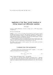
The idea <strong>of</strong> <strong>the</strong> shooting method <strong>of</strong> stepping over space and energy is<br />
explained in Fig. 1.<br />
Fig. 1. Algorithm <strong>of</strong> <strong>the</strong> shooting method. The internal cycle per<strong>for</strong>ms <strong>the</strong> stepping over space and<br />
two external cycles find <strong>the</strong> eigenvalues <strong>of</strong> <strong>the</strong> energy.<br />
251
2.3. The method <strong>of</strong> coupling <strong>the</strong> energy and wave functions<br />
As seen above, realization <strong>of</strong> <strong>the</strong> shooting method demands a ra<strong>the</strong>r small<br />
amount <strong>of</strong> computations but <strong>the</strong> definition <strong>of</strong> <strong>the</strong> boundary conditions and <strong>the</strong><br />
process <strong>of</strong> finding <strong>the</strong> exact energy eigenvalues need special care. Serious<br />
numerical problems may arise in <strong>the</strong> case <strong>of</strong> relatively thick barriers ( w >> 1 κ ),<br />
where exponential growth <strong>of</strong> <strong>the</strong> wave function follows from an inaccurately<br />
defined energy eigenvalue or discrepancies due to <strong>the</strong> limited number <strong>of</strong><br />
significant figures available <strong>for</strong> <strong>the</strong> arithmetic operations. To avoid <strong>the</strong>se<br />
problems, <strong>the</strong> EWC method was developed, which solves system <strong>of</strong> <strong>equation</strong>s<br />
with clearly fixed boundary conditions simultaneously <strong>for</strong> <strong>the</strong> energy eigenvalue<br />
and wave function values across <strong>the</strong> spatial grid nodes. The 3-point scheme <strong>of</strong><br />
spatial discretization used corresponds exactly to that <strong>of</strong> <strong>the</strong> shooting method<br />
in Eq. (5). The exact zero or cyclic boundary conditions <strong>for</strong> Ψ <strong>for</strong> <strong>the</strong> calculations<br />
are fixed. The zero boundary conditions actually correspond to <strong>the</strong> assumption<br />
about infinite potential barriers on <strong>the</strong> external borders <strong>of</strong> <strong>the</strong> calculation<br />
area. To find <strong>the</strong> energy eigenvalue toge<strong>the</strong>r with <strong>the</strong> values <strong>of</strong> <strong>the</strong> wave function<br />
on <strong>the</strong> grid nodes, an additional <strong>equation</strong> is necessary, besides <strong>the</strong> discretized<br />
Schrödinger <strong>equation</strong>, which is <strong>the</strong> normalization condition <strong>of</strong> <strong>the</strong> wave function<br />
(6). The latter states that <strong>the</strong> probability <strong>of</strong> finding an electron over <strong>the</strong><br />
entire space <strong>of</strong> <strong>the</strong> calculation equals unity. With this additional condition<br />
<strong>the</strong> calculated wave functions from <strong>the</strong> EWC method are automatically<br />
normalized.<br />
The unknown vector Y <strong>of</strong> <strong>the</strong> EWC method contains N components:<br />
<strong>the</strong> energy eigenvalue E and wave function values Ψi<br />
≡ Ψ ( xi<br />
) in nodes<br />
i= … 2, 3, , N <strong>of</strong> <strong>the</strong> grid:<br />
x = ( i−1) ∆x, ∆ x= L ( N − 1), i= 1, 2, ..., N,<br />
(10)<br />
i<br />
Y = ( E, Ψ , Ψ , ..., Ψ ) T<br />
N<br />
,<br />
(11)<br />
2 3<br />
where <strong>the</strong> superscript T denotes transposition.<br />
The value <strong>of</strong> <strong>the</strong> wave function in <strong>the</strong> 1st spatial node is not included in Y<br />
since<br />
Ψ = Ψ<br />
(12)<br />
1 N<br />
is assumed <strong>for</strong> both boundary condition types.<br />
The zero boundary conditions are <strong>the</strong>n specified simply as<br />
Ψ = 0.<br />
(13)<br />
N<br />
The cyclic boundary condition may be specified by <strong>the</strong> discrete Schrödinger<br />
<strong>equation</strong> (5) <strong>for</strong> <strong>the</strong> boundary node N . Taking into account <strong>the</strong> translational<br />
252
denotes<br />
̃ ̃ ̃ ̃<br />
is<br />
approach<br />
(19)<br />
and<br />
symmetry, <strong>the</strong> node N is equivalent to node 1, node N + 1 is equivalent to<br />
node 2 etc. Thus <strong>the</strong> necessary three “neighbour” wave function values in <strong>the</strong><br />
boundary node N are Ψ<br />
N 1 , −<br />
Ψ<br />
N<br />
= Ψ1 , Ψ 2 .<br />
Thus <strong>the</strong> first non-linear <strong>equation</strong> <strong>of</strong> <strong>the</strong> EWC method system is <strong>the</strong> rewritten<br />
normalization condition <strong>of</strong> <strong>the</strong> wave function (6) in discrete <strong>for</strong>m<br />
F( Ψ , Ψ , ..., Ψ ) ≡ Ψ ∆ − 1 = 0.<br />
1 2 3<br />
N<br />
N<br />
2<br />
∑ i<br />
x<br />
(14)<br />
i=<br />
2<br />
The next necessary N − 2 <strong>equation</strong>s are <strong>the</strong> discrete Schrödinger <strong>equation</strong>s<br />
(5) <strong>for</strong> <strong>the</strong> internal grid nodes i= 2, 3, ..., N − 1:<br />
2<br />
Ψi+ 1−Ψi Ψi −Ψi−<br />
1 1<br />
i( , Ψi− 1, Ψi, Ψi+<br />
1) ≡ − + ( − i) Ψi<br />
= 0,<br />
⎛<br />
⎞<br />
ħ<br />
⎜<br />
⎟<br />
F E<br />
2m ∆x ∆x ∆x<br />
E V<br />
(15)<br />
where <strong>for</strong> i = 2 according to Eq. (12) holds Ψi− 1 = Ψ<br />
N<br />
.<br />
In <strong>the</strong> case <strong>of</strong> zero boundary conditions, <strong>the</strong> last <strong>equation</strong> <strong>of</strong> <strong>the</strong> system is<br />
⎝<br />
⎠<br />
F ( Ψ ) ≡ Ψ = 0.<br />
(16)<br />
N N N<br />
In <strong>the</strong> case <strong>of</strong> <strong>the</strong> cyclic boundary condition, <strong>the</strong> last <strong>equation</strong> <strong>of</strong> <strong>the</strong> system is<br />
similar to Eq. (15) with <strong>the</strong> replacement Ψ<br />
1<br />
Ψ2 :<br />
N + =<br />
2<br />
Ψ2 −ΨN ΨN −ΨN−<br />
1 1<br />
N( , ΨN−1, ΨN, Ψ2) ≡ − + ( − N) ΨN<br />
= 0.<br />
⎛<br />
⎞<br />
ħ<br />
⎜<br />
⎟<br />
F E<br />
2m ∆x ∆x ∆x<br />
E V<br />
(17)<br />
The system (14)–(17) is non-linear as Eq. (14) contains squares <strong>of</strong> <strong>the</strong> values<br />
<strong>of</strong> <strong>the</strong> wave function and Eqs. (15) and (17) contain products <strong>of</strong> energy and wave<br />
functions. This system may be linearized and solved iteratively using <strong>the</strong> Newton<br />
method. For every iteration, <strong>the</strong> unknown vector Y may be written as<br />
⎝<br />
⎠<br />
̃<br />
Y = Y +δY,<br />
(18)<br />
̃<br />
[ ∂F ∂ Y] × δY =− F,<br />
Ỹ<br />
where <strong>the</strong> approximate unknown vector, δ Y is <strong>the</strong> correction vector,<br />
F ≡ ( F1, F2,..., F ) T<br />
<strong>the</strong> RHS vector <strong>of</strong> Ỹ<br />
<strong>the</strong> system calculated by<br />
[ ∂F<br />
∂ Y]<br />
is <strong>the</strong> N× N Jacobi matrix with <strong>the</strong> Newton method derivatives. In <strong>the</strong><br />
case <strong>of</strong> normal convergence, F̃<br />
both δ Y and to zero.<br />
The Jacobi matrix, obtained by differentiation <strong>of</strong> Eqs. (14)–(17), has a<br />
tridiagonal structure with filled first row and column and zero element in <strong>the</strong><br />
upper left corner. Four terms in <strong>the</strong> last line and <strong>the</strong> last column are not zero in<br />
<strong>the</strong> case <strong>of</strong> cyclic boundary conditions <strong>for</strong> Eq. (17):<br />
253
0 2Ψ 2Ψ 2Ψ 2 Ψ ... 2Ψ 2Ψ 2Ψ 2Ψ<br />
Ψ2 a2<br />
c 0 0 ... 0 0 0 c<br />
Ψ3 c a3<br />
c 0 ... 0 0 0 0<br />
Ψ4 0 c a4<br />
c ... 0 0 0 0<br />
... ... ... ... ... ... ... ... ... ...<br />
... ... ... ... ... ... ... ... ... ...<br />
... ... ... ... ... ... ... ... ... ...<br />
ΨN−<br />
2<br />
0 0 0 0 ... c aN<br />
−2<br />
c 0<br />
ΨN−1<br />
0 0 0 0 ... 0 c aN−1<br />
c<br />
Ψ c 0 0 0 ... 0 0 c a<br />
⎡<br />
⎢<br />
⎢<br />
⎢<br />
⎢<br />
⎢<br />
⎢<br />
⎢<br />
⎢<br />
⎢<br />
⎢<br />
⎢<br />
⎢<br />
⎢<br />
⎢<br />
⎣<br />
N<br />
2 3 4 5 N−3 N−2 N ⎤<br />
−1<br />
N<br />
2 2<br />
N<br />
⎥<br />
⎥<br />
⎥<br />
⎥<br />
⎥<br />
⎥<br />
⎥<br />
⎥<br />
⎥<br />
⎥<br />
⎥<br />
⎥<br />
⎥<br />
⎥<br />
,<br />
⎦<br />
(20)<br />
where c ≡ (2 m ħ ∆x<br />
) and ai<br />
≡E−Vi<br />
− 2. c<br />
In <strong>the</strong> case <strong>of</strong> zero boundary conditions <strong>of</strong> Eq. (16), in <strong>the</strong> last line <strong>of</strong> <strong>the</strong><br />
matrix (20) <strong>the</strong>re remains only one non-zero element a<br />
N<br />
= 1. A more radical way<br />
is to solve <strong>the</strong> problem with <strong>the</strong> ( N − 1) × ( N − 1) matrix without <strong>the</strong> last row and<br />
column <strong>for</strong> <strong>the</strong> respectively reduced unknown vector, since Ψ<br />
N<br />
= 0 is fixed and<br />
must not be considered as an unknown variable.<br />
To solve <strong>the</strong> linear system (19) with <strong>the</strong> tridiagonal bordered matrix (20), a<br />
special effective Gaussian elimination algorithm ([ 13 ], p 90) was applied.<br />
Using approximate <strong>for</strong>m <strong>for</strong> <strong>the</strong> wave function and <strong>the</strong> value <strong>of</strong> <strong>the</strong> energy<br />
level, <strong>the</strong> EWC method described here finds iteratively <strong>the</strong> exact value <strong>for</strong> energy<br />
and wave function <strong>for</strong> any specified potential. The approximate initial solution<br />
may be obtained from <strong>the</strong>oretical estimations or with any o<strong>the</strong>r method. The only<br />
drawback <strong>of</strong> <strong>the</strong> EWC method is that in <strong>the</strong> case <strong>of</strong> a poor initial approximation<br />
when, e.g., a wrong number <strong>of</strong> halfwaves <strong>of</strong> <strong>the</strong> wave function within <strong>the</strong> QW is<br />
determined, <strong>the</strong> convergence process may give a solution <strong>for</strong> a different eigenstate<br />
instead <strong>of</strong> <strong>the</strong> one which was wanted. The method was tested in <strong>the</strong> case <strong>of</strong><br />
MQW structures with hundreds <strong>of</strong> abrupt potential barriers [ 9 ]. A reliable scan<br />
over <strong>the</strong> whole range <strong>of</strong> eigenenergies was obtained if rough approximations<br />
were precalculated by <strong>the</strong> shooting method.<br />
Numerical tests showed that in <strong>the</strong> case <strong>of</strong> poor initial solutions <strong>the</strong> EWC<br />
method usually needed 5–7 iterations to converge. Divergence was never<br />
observed. In a combined use toge<strong>the</strong>r with <strong>the</strong> shooting method, <strong>the</strong> typical<br />
number <strong>of</strong> Newton iterations decreased to 3–4 to reach convergence with<br />
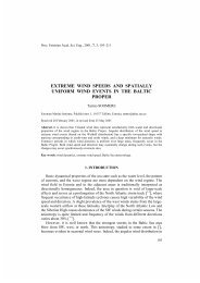
practically zero error. Figure 2 illustrates very high quadratic convergence speed<br />
<strong>of</strong> <strong>the</strong> EWC method.<br />
254
Iteration<br />
Fig. 2. Typical convergence characteristics <strong>of</strong> <strong>the</strong> iteration process <strong>of</strong> <strong>the</strong> EWC method. Figure<br />
shows in logarithmic scale <strong>the</strong> decrease <strong>of</strong> <strong>the</strong> bound state energy increment δE (eV), <strong>the</strong> decrease<br />
<strong>of</strong> <strong>the</strong> maximum relative wave function increment and <strong>the</strong> approach <strong>of</strong> <strong>the</strong> particle finding<br />
probability to its <strong>the</strong>oretical limit <strong>of</strong> 1.<br />
3. RESULTS OF THE EFFICIENCY TEST<br />
3.1. <strong>Comparison</strong> <strong>of</strong> <strong>the</strong> accuracy <strong>of</strong> <strong>the</strong> FGH and EWC <strong>methods</strong><br />
Prior to comparing <strong>the</strong> efficiency on <strong>the</strong> basis <strong>of</strong> consumption <strong>of</strong> <strong>the</strong> computer<br />
time, an estimation <strong>of</strong> equivalent spatial grid sizes should be per<strong>for</strong>med. Some<br />
preliminary calculations in <strong>the</strong> case <strong>of</strong> a nearly sine wave function showed that<br />
minimal rough accuracy may be achieved with <strong>the</strong> FGH method if <strong>the</strong> number <strong>of</strong><br />
grid nodes per wave <strong>of</strong> Ψ is 2–3. For EWC method <strong>the</strong> corresponding number<br />
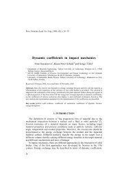
was 4–5. A more accurate comparison was per<strong>for</strong>med <strong>for</strong> a triple QW task as<br />
described in Fig. 3.<br />
The structure in Fig. 3 has three quantum wells <strong>of</strong> 9 Å width and 10 eV<br />
depth, separated by 1 Å barriers. The size <strong>of</strong> <strong>the</strong> outer barriers on both sides is<br />
9 Å. The structure has 15 energy levels below 10 eV. The separation <strong>of</strong> energy<br />
levels has peculiarities and <strong>the</strong> wave functions contain intervals with different<br />
spatial frequencies. In tests, <strong>the</strong> free electron rest mass was used. To achieve<br />
maximum compatibility between <strong>the</strong> FGH and EWC <strong>methods</strong>, which use<br />
slightly different localization <strong>of</strong> spatial grid nodes, special care was taken.<br />
Additionally, <strong>for</strong> <strong>the</strong> border nodes in <strong>the</strong> FGH method a high potential energy<br />
255
Coordinate, Å<br />
Fig. 3. Potential energy (▬) and 15 calculated wave functions (—) in <strong>the</strong> triple quantum well<br />
test structure. The variable part <strong>of</strong> wave functions is presented in an arbitrary scale but <strong>the</strong><br />
average values are fixed in accordance to <strong>the</strong> corresponding energy level. Free electron rest mass is<br />
used.<br />
value was assigned to model <strong>the</strong> zero boundary conditions <strong>of</strong> <strong>the</strong> EWC method.<br />
In this comparison <strong>the</strong> accuracy <strong>of</strong> both <strong>methods</strong> was evaluated by a comparison<br />
<strong>of</strong> <strong>the</strong> accuracy <strong>of</strong> <strong>the</strong> energy eigenvalues calculations. Since <strong>the</strong> computer time<br />
consumption <strong>of</strong> <strong>the</strong> FGH method became very high <strong>for</strong> greater grid point<br />
numbers, exact reference numbers were obtained with <strong>the</strong> EWC method <strong>for</strong> <strong>the</strong><br />
grid with N = 30 000. The accuracy criterion <strong>for</strong> finishing <strong>the</strong> Newton iterations<br />
−9<br />
in <strong>the</strong> EWC method was practically set to zero ( δ E ≤ 10 eV). The results are<br />
presented in Fig. 4.<br />
As Fig. 4 shows, <strong>for</strong> both <strong>methods</strong> <strong>the</strong> error <strong>of</strong> energy level decreases with <strong>the</strong><br />
grid step as ∼∆ x 2 . However, to achieve a comparable accuracy, <strong>the</strong> EWC<br />
method needs approximately three times more grid nodes. For example, a<br />
relatively good accuracy <strong>of</strong> 0.1 meV needs approximately 1500 nodes in <strong>the</strong> case<br />
<strong>of</strong> <strong>the</strong> FGH method and 4500 nodes in <strong>the</strong> case <strong>of</strong> <strong>the</strong> EWC method.<br />
256
Error <strong>of</strong> E, meV<br />
Grid step ∆x, Å<br />
Fig. 4. The accuracy <strong>of</strong> calculated energy eigenvalues versus grid step <strong>for</strong> FGH and EWC <strong>methods</strong>.<br />
The triple QW structure (Fig. 3) is tested. The maximum error and <strong>the</strong> root mean square error <strong>for</strong><br />
<strong>the</strong> set <strong>of</strong> 15 energy levels are shown.<br />
3.2. <strong>Comparison</strong> <strong>of</strong> computation times <strong>of</strong> <strong>the</strong> FGH and EWC <strong>methods</strong><br />
The computer times <strong>for</strong> both approaches are compared in Fig. 5. The calculations<br />
were per<strong>for</strong>med <strong>for</strong> a triple QW structure with 15 energy levels according<br />
to Fig. 3. As <strong>the</strong> approximate wave functions and energy eigenvalues <strong>for</strong> <strong>the</strong><br />
EWC method were calculated by shooting method, <strong>the</strong> corresponding results are<br />
marked as ShM + EWC in Fig. 5. In <strong>the</strong> case <strong>of</strong> <strong>the</strong> FGH method, <strong>the</strong> computer<br />
time practically depends only on <strong>the</strong> number <strong>of</strong> grid points and not on <strong>the</strong> <strong>for</strong>m <strong>of</strong><br />
<strong>the</strong> potential. In <strong>the</strong> case <strong>of</strong> <strong>the</strong> EWC method, <strong>the</strong> amount <strong>of</strong> computer time is<br />
also proportional to <strong>the</strong> number <strong>of</strong> energy levels. Numerical experiments were<br />
per<strong>for</strong>med on a desktop PC with a 3 GHz Pentium-4 processor on Windows XP<br />
plat<strong>for</strong>m using GNU-Fortran-77 programming language.<br />
3<br />
Figure 5 shows <strong>the</strong> tcomp<br />
∼ N dependence <strong>of</strong> <strong>the</strong> FGH method. That limits <strong>the</strong><br />
practical use <strong>of</strong> this method to <strong>the</strong> grid sizes from 2000 to 3000. It is interesting<br />
that <strong>the</strong> reduced version <strong>of</strong> <strong>the</strong> FGH, which does not calculate <strong>the</strong> wave<br />
functions, does not significantly reduce <strong>the</strong> computational time. In contrast to <strong>the</strong><br />
FGH, in <strong>the</strong> case <strong>of</strong> <strong>the</strong> EWC method t comp depends linearly on N . Although <strong>the</strong><br />
EWC method needs roughly three times more grid nodes <strong>for</strong> <strong>the</strong> same accuracy,<br />
257
Computer time, s<br />
Number <strong>of</strong> grid nodes, N<br />
Fig. 5. <strong>Comparison</strong> <strong>of</strong> <strong>the</strong> computer times versus grid size <strong>for</strong> FGH and EWC <strong>methods</strong>. The latter is<br />
completed with ShM, which provides approximate energy values and wave functions. Triple QW<br />
structure with 15 bound state energy levels (Fig. 3) is tested.<br />
<strong>the</strong> comparison proves clearly that <strong>the</strong> ShM + EWC approach is more than three<br />
orders <strong>of</strong> magnitudes more effective than <strong>the</strong> FGH method. Computer times <strong>of</strong><br />
subsecond range show that <strong>the</strong> ECW method may be easily applied to very<br />
5<br />
complex MQW problems that demand 10 and more grid nodes.<br />
Some tests were also per<strong>for</strong>med with <strong>the</strong> shooting method on its own.<br />
However, <strong>the</strong> exact results <strong>of</strong> a comparison between <strong>the</strong> ShM and <strong>the</strong> combined<br />
ShM + EWC method depend on <strong>the</strong> specific finishing criteria <strong>for</strong> <strong>the</strong> coordinate<br />
and energy iteration processes in <strong>the</strong> ShM. The EWC method is ra<strong>the</strong>r insensitive<br />
in <strong>the</strong> sense that its boundary conditions are clearly fixed and <strong>the</strong> energy<br />
convergence speed is very high (Fig. 2). Numerical experiments showed that by<br />
careful selection <strong>of</strong> <strong>the</strong> accuracy criteria and using <strong>the</strong> benefit <strong>of</strong> a symmetric<br />
structure, it was possible to obtain 30–40% shorter computer times with <strong>the</strong> pure<br />
ShM. However, in <strong>the</strong> general case <strong>of</strong> a non-symmetrical structure and guaranteed<br />
high accuracy <strong>the</strong> combined ShM + EWC approach was approximately 1.5–2<br />
times more effective than <strong>the</strong> use <strong>of</strong> <strong>the</strong> ShM only.<br />
258
4. DISCUSSION AND CONCLUSIONS<br />
We have discussed and tested qualitatively some practical approaches to <strong>the</strong><br />
solution <strong>of</strong> <strong>the</strong> time-independent 1D Schrödinger <strong>equation</strong> without any restrictions<br />
on <strong>the</strong> potential energy distribution. The comparison was centred around<br />
two effective <strong>methods</strong>: <strong>the</strong> Fourier grid Hamiltonian method known from <strong>the</strong><br />
field <strong>of</strong> physical chemistry and <strong>the</strong> shooting method <strong>of</strong>ten applied to semiconductor<br />
quantum well calculations. We established cubic computer time<br />
dependence on <strong>the</strong> number <strong>of</strong> grid points in <strong>the</strong> FGH method and concluded that<br />
it is very difficult to use this method <strong>for</strong> complex tasks which need more than<br />
2000 grid points.<br />
We also critically analysed <strong>the</strong> drawbacks <strong>of</strong> extremely simple trial-andcorrection<br />
type shooting <strong>methods</strong> and <strong>of</strong>fered a more general and reliable<br />
coupled energy and wave function method (EWC) with a Newton iteration<br />
scheme and an internal linear task with a tridiagonal bordered matrix. We<br />
<strong>for</strong>mulated this EWC method <strong>for</strong> two types <strong>of</strong> boundary conditions: zero wave<br />
function (hard wall) or cyclic. A survey <strong>of</strong> <strong>the</strong> literature showed that <strong>the</strong> EWC<br />
method was actually an extended version <strong>of</strong> a relaxational approach [ 4 ] published<br />
in 2001.<br />
For versatile multiquantum well problems we developed an effective and<br />
reliable combined approach (ShM + EWC) where at first <strong>the</strong> shooting method is<br />
used <strong>for</strong> a rough estimation <strong>of</strong> <strong>the</strong> energy eigenvalues and approximate wave<br />
functions. Secondly, <strong>the</strong> fast-converging EWC method is applied <strong>for</strong> reliable<br />
calculation <strong>of</strong> more exact results. Detailed investigation <strong>of</strong> <strong>the</strong> grid error and<br />
computer time on <strong>the</strong> basis <strong>of</strong> a triple quantum well task <strong>for</strong> both <strong>the</strong> FGH and<br />
ShM + EWC approaches was per<strong>for</strong>med. The results show that although <strong>the</strong><br />
ShM + EWC method needs approximately three times more grid nodes than <strong>the</strong><br />
FGH method, it is still several orders <strong>of</strong> magnitudes more effective than <strong>the</strong> FGH<br />
5<br />
method. On modern computers, MQW tasks with grid point numbers over 10<br />
may be easily solved with <strong>the</strong> EWC method.<br />
ACKNOWLEDGEMENTS<br />
This work has been partly supported by <strong>the</strong> Estonian Science Foundation<br />
(grant No. 5911). Paul Harrison would like to thank <strong>the</strong> Faculty <strong>of</strong> Engineering<br />
<strong>of</strong> <strong>the</strong> University <strong>of</strong> Leeds <strong>for</strong> financial support. The authors are grateful to<br />
Dr. Zoran Ikonić from University <strong>of</strong> Leeds <strong>for</strong> valuable comments on <strong>the</strong><br />
algorithms <strong>for</strong> <strong>solving</strong> <strong>the</strong> Schrödinger <strong>equation</strong>.<br />
REFERENCES<br />
1. Marston, C. C. and Balint-Kurti, G. G. The Fourier grid Hamiltonian method <strong>for</strong> bound state<br />
eigenvalues and eigenfunctions. J. Chem. Phys. Rev., 1989, 91, 3571–3576.<br />
259
2. Balint-Kurti, G. G. and Ward, C. L. Two computer programs <strong>for</strong> <strong>solving</strong> <strong>the</strong> Schrödinger<br />
<strong>equation</strong> <strong>for</strong> bound-state eigenvalues and eigenfunctions using <strong>the</strong> Fourier grid Hamiltonian<br />
method. Comput. Phys. Comm., 1991, 67, 285–292.<br />
3. Balint-Kurti, G. G., Dixon, R. N. and Marston, C. C. Grid <strong>methods</strong> <strong>for</strong> <strong>solving</strong> <strong>the</strong> Schrödinger<br />
<strong>equation</strong> and time dependent quantum dynamics <strong>of</strong> molecular phot<strong>of</strong>ragmentation and<br />
reactive scattering processes. Internat. Rev. Phys. Chem., 1992, 11, 317–344.<br />
4. Praeger, J. D. Relaxational approach to <strong>solving</strong> <strong>the</strong> Schrödinger <strong>equation</strong>. Phys. Rev. A, 2001,<br />
63, 022115, 10 p.<br />
5. Nakanishi, H. and Sugawara, M. Numerical solution <strong>of</strong> <strong>the</strong> Schrödinger <strong>equation</strong> by a microgenetic<br />
algorithm. Chem. Phys. Lett., 2000, 327, 429–438.<br />
6. Selg, M. Numerically complemented analytic method <strong>for</strong> <strong>solving</strong> <strong>the</strong> time-independent onedimensional<br />
Schrödinger <strong>equation</strong>. Phys. Rev. E, 2001, 64, 056701, 12 p.<br />
7. Harrison, P. Quantum Wells, Wires and Dots. Wiley, Chichester, 2002.<br />
8. Indjin, D., Tomic, S., Ikonic, Z., Harrison, P., Kelsall, R. W., Milanovic, V. and Kocinac, S.<br />
Gain-maximized GaAs/AlGaAs quantum cascade laser with digitally graded active region.<br />
Appl. Phys. Lett., 2002, 81, 2163–2165.<br />
9. Reeder, R., Udal, A., Velmre, E. and Harrison, P. Numerical investigation <strong>of</strong> digitised parabolic<br />
quantum wells <strong>for</strong> terahertz AlGaAs/GaAs structures. In Proc. Baltic Electronic<br />
Conference BEC2006. Tallinn, 2006, 4 p. Forthcoming.<br />
10. EISPACK package <strong>of</strong> Fortran subroutines that compute <strong>the</strong> eigenvalues and eigenvectors <strong>of</strong><br />
matrices (developed in 1972–73), http://www.netlib.org/eispack/<br />
11. University <strong>of</strong> Bristol, Centre <strong>for</strong> Computational Chemistry, http://www.chm.bris.ac.uk/pt/ggbk/<br />
gabriel.htm<br />
12. Brau, F. and Semay, C. The 3-dimensional Fourier grid Hamiltonian method. J. Computat.<br />
Phys., 1998, 139, 127–136.<br />
13. Samarski, A. A. and Nikolajev, E. S. Solution Methods <strong>for</strong> Finite Difference Equations. Nauka,<br />
Moscow, 1978 (in Russian).<br />
260<br />
Schrödingeri võrrandi lahendusmeetodite võrdlus<br />
mitmik-kvantaukudega heterostruktuuride jaoks<br />
Andres Udal, Reeno Reeder, Enn Velmre ja Paul Harrison<br />
On võrreldud otseseid numbrilisi lahendusmeetodeid ajast sõltumatu ühemõõtmelise<br />
Schrödingeri võrrandi lahendamiseks. Mitmik-kvantaukudega (MQW)<br />
pooljuht-heterostruktuuride arvutused nõuavad meetodeid, mille puhul arvutusaeg<br />
t comp sõltub ruumivõrgu sammude arvust N lineaarselt. Tuntud ja väga efektiivseks<br />
peetav Fourier Grid Hamiltoniani (FGH) meetod (Fourier’ teisenduse ja ruumivõrgu<br />
alusel moodustatud hamiltoniaani analüüsiv meetod) omab aga kuupsõltuvust<br />
t comp ~ N 3 , mistõttu selle meetodi rakendusala on piiratud probleemidega,<br />
kus N ≤ 1000 on piisav. Lihtsaim otsene lahendusmeetod on nn tulistamismeetod<br />
(ShM), mis põhineb katselisel astumisel üle ruumikoordinaadi ja energiaväärtuste.<br />
Tulistamismeetod omab vajalikku lineaarset sõltuvust t comp ~ N ja rahuldavat<br />
energiaväärtuste koondumiskiirust, kuid ebaselgelt määratletud piiritingimused<br />
teevad meetodi kasutamise ebamugavaks. Artiklis on esitatud energianivoode ja<br />
lainefunktsioonide kooslahendamise meetod (EWC), mis on töökindel ja efektiivne<br />
ning omab lineaarset sõltuvust t comp ~ N. Meetod põhineb mittelineaarsete võrrandisüsteemide<br />
lahendamiseks sobival Newtoni iteratsioonimeetodil, kusjuures sise-
mise lineaarse ülesandena lahendatakse kolmediagonaalse ääristatud maatriksiga<br />
süsteem. Esitatud meetod on rakendatav suvalise potentsiaalse energia jaotusega<br />
ülesannetele keerukusega N = 10 5 ja üle selle nii nulliliste kui ka tsükliliste piiritingimuste<br />
puhul. Praktiliste MQW-ülesannete jaoks on realiseeritud võimalus<br />
kasutada meetodeid kombineeritult, mille puhul arvutatakse ShM-i abil energiate ja<br />
lainefunktsioonide ligikaudsed alglähendid väga kiirelt koonduvale EWC-meetodile.<br />
Kolmik-kvantaugu näitel <strong>for</strong>muleeritud testülesande lahendamise teel on<br />
võrreldud vaadeldud meetodite ruumilist täpsust ja arvutiaega. Tulemused näitavad,<br />
et kombineeritud meetod ShM + EWC on FGH-meetodist mitu suurusjärku<br />
efektiivsem.<br />
261