Application of the Haar wavelet transform to solving integral and ...
Application of the Haar wavelet transform to solving integral and ...
Application of the Haar wavelet transform to solving integral and ...

Create successful ePaper yourself
Turn your PDF publications into a flip-book with our unique Google optimized e-Paper software.
Proc. Es<strong>to</strong>nian Acad. Sci. Phys. Math., 2007, 56, 1, 28–46<br />
<strong>Application</strong> <strong>of</strong> <strong>the</strong> <strong>Haar</strong> <strong>wavelet</strong> <strong>transform</strong> <strong>to</strong><br />
<strong>solving</strong> <strong>integral</strong> <strong>and</strong> differential equations<br />
Ülo Lepik<br />
Institute <strong>of</strong> Applied Ma<strong>the</strong>matics, University <strong>of</strong> Tartu, Liivi 2, 50409 Tartu, Es<strong>to</strong>nia;<br />
ulo.lepik@ut.ee<br />
Received 13 November 2006<br />
Abstract. A survey on <strong>the</strong> use <strong>of</strong> <strong>the</strong> <strong>Haar</strong> <strong>wavelet</strong> method for <strong>solving</strong> nonlinear <strong>integral</strong><br />
<strong>and</strong> differential equations is presented. This approach is applicable <strong>to</strong> different kinds <strong>of</strong><br />
<strong>integral</strong> equations (Fredholm, Volterra, <strong>and</strong> integro-differential equations). <strong>Application</strong> <strong>to</strong><br />
partial differential equations is exemplified by <strong>solving</strong> <strong>the</strong> sine-Gordon equation. All <strong>the</strong>se<br />
problems are solved with <strong>the</strong> aid <strong>of</strong> collocation techniques.<br />
Computer simulation is carried out for problems <strong>the</strong> exact solution <strong>of</strong> which is known. This<br />
allows us <strong>to</strong> estimate <strong>the</strong> precision <strong>of</strong> <strong>the</strong> obtained numerical results. High accuracy <strong>of</strong> <strong>the</strong><br />
results even in <strong>the</strong> case <strong>of</strong> a small number <strong>of</strong> collocation points is observed.<br />
Key words: <strong>integral</strong> equations, evolution equations, <strong>Haar</strong> <strong>wavelet</strong> method, sine-Gordon<br />
equation, collocation method.<br />
1. INTRODUCTION AND BACKGROUND<br />
Let us first explain why we need <strong>wavelet</strong>s at all. A signal x = x(t) is <strong>of</strong>ten<br />
analysed with <strong>the</strong> aid <strong>of</strong> <strong>the</strong> Fourier <strong>transform</strong><br />
F (ω) =<br />
∫ +∞<br />
−∞<br />
x(t)e −iωt dt, (1)<br />
where ω denotes <strong>the</strong> frequency <strong>and</strong> F – <strong>the</strong> amplitude.<br />
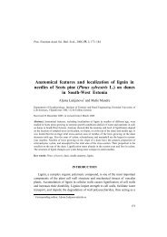
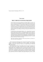
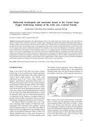
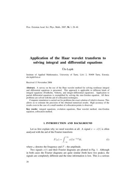
Two signals x(t) <strong>and</strong> <strong>the</strong>ir Fourier diagrams are plotted in Fig. 1. Although<br />
in both cases <strong>the</strong> Fourier diagrams are quite similar (both have two peaks), <strong>the</strong><br />
signals are completely different <strong>and</strong> <strong>the</strong> time information is lost. This is a serious<br />
28
2<br />
(a)<br />
1<br />
50<br />
x<br />
0<br />
IFI<br />
30<br />
1<br />
10<br />
2<br />
0 2 4 6 8 10<br />
0.5<br />
(b)<br />
1<br />
t<br />
0<br />
0<br />
30<br />
25<br />
20 40 60<br />
t<br />
x<br />
0<br />
IFI<br />
20<br />
15<br />
0.5<br />
1<br />
0 2 4 6 8 10<br />
t<br />
10<br />
5<br />
0<br />
0<br />
20 40 60<br />
t<br />
Fig. 1. Time his<strong>to</strong>ry <strong>and</strong> Fourier diagram for (a) x = sin 3t + 0.8 sin 10t for t ∈ [0, 10]<br />
<strong>and</strong> (b) x = sin 3t for t ∈ [0, 5], x = sin 10t for t ∈ [5, 10].<br />
drawback: <strong>the</strong> Fourier method analyses <strong>the</strong> signal over <strong>the</strong> whole domain <strong>and</strong> is<br />
unable <strong>to</strong> characterize its behaviour in time.<br />
Wavelet analysis allows us <strong>to</strong> represent a function in terms <strong>of</strong> a set <strong>of</strong> basic<br />
functions, called <strong>wavelet</strong>s, which are localized both in space <strong>and</strong> time. Here a<br />
continuous function ψ(t), called <strong>the</strong> mo<strong>the</strong>r <strong>wavelet</strong>, is introduced. The corresponding<br />
<strong>wavelet</strong> family is formed by <strong>the</strong> dilation <strong>and</strong> translation <strong>of</strong> <strong>the</strong> function<br />
ψ(t):<br />
ψ j,k (t) = 2 −j/2 ψ(2 −j t − k), (2)<br />
where j <strong>and</strong> k are non-negative integers.<br />
Depending upon <strong>the</strong> choice <strong>of</strong> <strong>the</strong> mo<strong>the</strong>r <strong>wavelet</strong> ψ(t), various <strong>wavelet</strong><br />
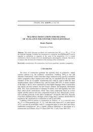
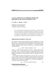
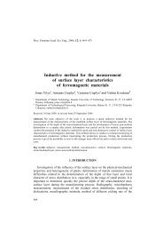
families are obtained. The <strong>wavelet</strong>s introduced by Daubechies [ 1 ] are quite<br />
frequently used for <strong>solving</strong> different problems. The Daubechies mo<strong>the</strong>r <strong>wavelet</strong><br />
is plotted in Fig. 2. These <strong>wavelet</strong>s are differentiable <strong>and</strong> have a minimum size<br />
support.<br />
A shortcoming <strong>of</strong> <strong>the</strong> Daubechies <strong>wavelet</strong>s is that <strong>the</strong>y do not have an explicit<br />
expression <strong>and</strong> <strong>the</strong>refore analytical differentiation or integration is not possible.<br />
This complicates <strong>the</strong> solution <strong>of</strong> differential equations where <strong>integral</strong>s <strong>of</strong> <strong>the</strong><br />
following type<br />
∫ b<br />
(<br />
G t, ψ i,k , dψ )<br />
i,k<br />
, d2 ψ i,k<br />
dt dt 2 , ... dt (3)<br />
a<br />
must be computed (G is generally a nonlinear function). For calculating such<br />
<strong>integral</strong>s <strong>the</strong> conception <strong>of</strong> connection coefficients is introduced. Calculation <strong>of</strong><br />
29
1<br />
ψ<br />
0<br />
-1<br />
2 4 6 8 10<br />
t<br />
Fig. 2. Daubechies mo<strong>the</strong>r <strong>wavelet</strong> <strong>of</strong> order J = 6.<br />
<strong>the</strong>se coefficients is very complicated <strong>and</strong> must be carried out separately for<br />
different types <strong>of</strong> <strong>integral</strong>s (see, e.g., [ 2 ]). Besides, it can be done only for some<br />
simpler types <strong>of</strong> nonlinearities (mainly for quadratic nonlinearity). This remark<br />
holds also for o<strong>the</strong>r types <strong>of</strong> <strong>wavelet</strong>s (such as Symlet, Coiflet, etc. <strong>wavelet</strong>s).<br />
The <strong>wavelet</strong> method was first applied <strong>to</strong> <strong>solving</strong> differential <strong>and</strong> <strong>integral</strong><br />
equations in <strong>the</strong> 1990s. A survey <strong>of</strong> early results in this field can be found in [ 3 ].<br />
Lately <strong>the</strong> number <strong>of</strong> respective papers has greatly increased <strong>and</strong> it is not possible<br />
<strong>to</strong> analyse <strong>the</strong>m all here, but some are discussed in <strong>the</strong> following sections.<br />
Due <strong>to</strong> <strong>the</strong> complexity <strong>of</strong> <strong>the</strong> <strong>wavelet</strong> solutions, some pessimistic estimates<br />
exist. So Strang <strong>and</strong> Nguyen write in <strong>the</strong>ir text-book [ 4 ] “... <strong>the</strong> competition with<br />
o<strong>the</strong>r methods is severe. We do not necessarily predict that <strong>wavelet</strong>s will win”<br />
(p. 394). Jameson [ 5 ] writes “... nonlinearities etc., when treated in a <strong>wavelet</strong><br />
subspace, are <strong>of</strong>ten unnecessarily complicated ... There appears <strong>to</strong> be no compelling<br />
reason <strong>to</strong> work with Galerkin-style coefficients in a <strong>wavelet</strong> method” (p. 1982).<br />
Obviously attempts <strong>to</strong> simplify solutions based on <strong>the</strong> <strong>wavelet</strong> approach are<br />
wanted. One possibility is <strong>to</strong> make use <strong>of</strong> <strong>the</strong> <strong>Haar</strong> <strong>wavelet</strong> family.<br />
In 1910 Alfred <strong>Haar</strong> introduced a function which presents a rectangular pulse<br />
pair. After that various generalizations were proposed (a state <strong>of</strong> <strong>the</strong> art about <strong>Haar</strong><br />
<strong>transform</strong>s can be found in [ 6 ]). In <strong>the</strong> 1980s it turned out that <strong>the</strong> <strong>Haar</strong> function was<br />
in fact <strong>the</strong> Daubechies <strong>wavelet</strong> <strong>of</strong> order 1. It is <strong>the</strong> simplest orthonormal <strong>wavelet</strong><br />
with compact support.<br />
The <strong>Haar</strong> <strong>wavelet</strong> family is defined for t ∈ [0, 1] as follows:<br />
⎧<br />
⎨ 1 for t ∈ [ξ 1 , ξ 2 ) ,<br />
h i (t) = −1 for t ∈ [ξ 2 , ξ 3 ] ,<br />
⎩<br />
0 elsewhere .<br />
Here ξ 1 = k/m , ξ 2 = (k + 0.5)/m , ξ 3 = (k + 1)m . The integer m = 2 j<br />
(j = 0, 1, ..., J) indicates <strong>the</strong> level <strong>of</strong> <strong>the</strong> <strong>wavelet</strong>; k = 0, 1, ..., m − 1 is <strong>the</strong><br />
translation parameter. The maximal level <strong>of</strong> resolution is J. The index i in (4) is<br />
(4)<br />
30
calculated according <strong>to</strong> <strong>the</strong> formula i = m + k + 1; in <strong>the</strong> case m = 1, k = 0 we<br />
have i = 2; <strong>the</strong> maximal value <strong>of</strong> i is i = 2M = 2 J+1 . It is assumed that <strong>the</strong> value<br />
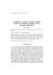
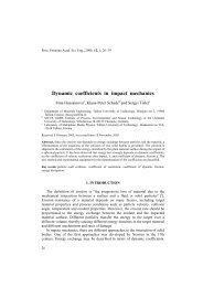
i = 1 corresponds <strong>to</strong> <strong>the</strong> scaling function for which h 1 = 1 for t ∈ [0, 1]. The first<br />
eight <strong>Haar</strong> functions are plotted in Fig. 3.<br />
An essential shortcoming <strong>of</strong> <strong>the</strong> <strong>Haar</strong> <strong>wavelet</strong>s is that <strong>the</strong>y are not continuous.<br />
The derivatives do not exist in <strong>the</strong> points <strong>of</strong> discontinuity, <strong>the</strong>refore it is not possible<br />
<strong>to</strong> apply <strong>the</strong> <strong>Haar</strong> <strong>wavelet</strong>s directly <strong>to</strong> <strong>solving</strong> differential equations.<br />
There are at least two possibilities <strong>of</strong> ending this impasse. First, <strong>the</strong> piecewise<br />
constant <strong>Haar</strong> functions can be regularized with interpolation splines; this<br />
technique has been applied by Cattani [ 7,8 ]. This greatly complicates <strong>the</strong> solution<br />
process <strong>and</strong> <strong>the</strong> main advantage <strong>of</strong> <strong>the</strong> <strong>Haar</strong> <strong>wavelet</strong>s – <strong>the</strong>ir simplicity – gets lost.<br />
Ano<strong>the</strong>r possibility was proposed by Chen <strong>and</strong> Hsiao [ 9,10 ]. They<br />
recommended <strong>to</strong> exp<strong>and</strong> in<strong>to</strong> <strong>the</strong> <strong>Haar</strong> series not <strong>the</strong> function itself, but its<br />
highest derivative appearing in <strong>the</strong> differential equation; <strong>the</strong> o<strong>the</strong>r derivatives (<strong>and</strong><br />
<strong>the</strong> function) are obtained through integrations. All <strong>the</strong>se ingredients are <strong>the</strong>n<br />
incorporated in<strong>to</strong> <strong>the</strong> whole system, discretized by <strong>the</strong> Galerkin or collocation<br />
method.<br />
Chen <strong>and</strong> Hsiao demonstrated <strong>the</strong> possibilities <strong>of</strong> <strong>the</strong>ir method by <strong>solving</strong> linear<br />
systems <strong>of</strong> ordinary differential equations (ODEs) <strong>and</strong> partial differential equations<br />
(PDEs). In [ 10 ] an optimal control problem with <strong>the</strong> quadratic performance index<br />
is discussed.<br />
In [ 11,12 ] Hsiao <strong>and</strong> Wang applied this method <strong>to</strong> <strong>solving</strong> singular bilinear <strong>and</strong><br />
nonlinear systems. Nonlinear stiff systems were examined in [ 13 ].<br />
In [ 14 ] Hsiao demonstrated that <strong>the</strong> <strong>Haar</strong> <strong>wavelet</strong> approach is effective also<br />
for <strong>solving</strong> variational problems. Of importance is also <strong>the</strong> paper [ 15 ] by Hsiao<br />
Fig. 3. The first eight <strong>Haar</strong> functions.<br />
31
<strong>and</strong> Rathsfeld, in which <strong>wavelet</strong> collocation methods are applied <strong>to</strong> <strong>the</strong> boundary<br />
element solution <strong>of</strong> <strong>the</strong> first-kind <strong>integral</strong> equations arising in acoustic scattering.<br />
The aim <strong>of</strong> <strong>the</strong> present paper is <strong>to</strong> acquaint <strong>the</strong> readers with <strong>the</strong> possibilities<br />
<strong>of</strong> <strong>the</strong> <strong>Haar</strong> <strong>wavelet</strong> method in <strong>solving</strong> <strong>integral</strong> <strong>and</strong> evolution equations. The<br />
illustrating examples are taken from papers published by <strong>the</strong> author.<br />
2. INTEGRATION OF HAAR WAVELETS<br />
If we want <strong>to</strong> integrate differential equations by <strong>the</strong> Hsiao–Chen method, we<br />
have <strong>to</strong> evaluate <strong>the</strong> <strong>integral</strong>s<br />
p i,ν (t) =<br />
p i,1 (t) =<br />
∫ t<br />
0<br />
∫ t<br />
0<br />
h i (t)dt,<br />
p i,ν−1 (t)dt, ν = 2, 3, ... .<br />
Carrying out <strong>the</strong>se integrations with <strong>the</strong> aid <strong>of</strong> (4), we find<br />
⎧<br />
⎨ t − ξ 1 for t ∈ [ξ 1 , ξ 2 ] ,<br />
p i,1 (t) = ξ 3 − t for t ∈ [ξ 2 , ξ 3 ] ,<br />
⎩<br />
0 elsewhere;<br />
⎧<br />
32<br />
⎪⎨<br />
p i,2 (t) =<br />
⎧<br />
⎪⎨<br />
p i,3 (t) =<br />
⎧<br />
⎪⎨<br />
p i,4 (t) =<br />
⎪⎩<br />
⎪⎩<br />
⎪⎩<br />
0 for t ∈ [0, ξ 1 ] ,<br />
1<br />
2 (t − ξ 1) 2 for t ∈ [ξ 1 , ξ 2 ] ,<br />
1<br />
4m 2 − 1 2 (ξ 3 − t) 2 for t ∈ [ξ 2 , ξ 3 ] ,<br />
1<br />
4m 2 for t ∈ [ξ 3 , 1] ;<br />
0 for t ∈ [0, ξ 1 ] ,<br />
1<br />
6 (t − ξ 1) 3 for t ∈ [ξ 1 , ξ 2 ] ,<br />
1<br />
4m 2 (t − ξ 2) + 1 6 (ξ 3 − t) 3 for t ∈ [ξ 2 , ξ 3 ] ,<br />
1<br />
4m 2 (t − ξ 2) for t ∈ [ξ 3 , 1] ;<br />
0 for t ∈ [0, ξ 1 ] ,<br />
1<br />
24 (t − ξ 1) 4 for t ∈ [ξ 1 , ξ 2 ] ,<br />
1<br />
8m 2 (t − ξ 2) 2 − 1<br />
24 (ξ 3 − t) 4 + 1<br />
192m 4 for t ∈ [ξ 2 , ξ 3 ] ,<br />
1<br />
8m 2 (t − ξ 2) 2 + 1<br />
192m 4 for t ∈ [ξ 3 , 1] .<br />
(5)<br />
(6)
It is necessary <strong>to</strong> evaluate <strong>the</strong>se functions for a prescribed J only once <strong>and</strong> save<br />
<strong>the</strong>m in <strong>the</strong> s<strong>to</strong>rage <strong>of</strong> <strong>the</strong> computer.<br />
It is convenient <strong>to</strong> pass <strong>to</strong> <strong>the</strong> matrix formulation. For this purpose <strong>the</strong> interval<br />
t ∈ [0, 1] is divided in<strong>to</strong> 2M parts <strong>of</strong> equal length ∆t = 1/2M, where M = 2 J .<br />
The grid points are<br />
t(l) = (l − 0.5)∆t, l = 1, 2, ..., 2M. (7)<br />
The <strong>Haar</strong> coefficient matrix H is defined as H(i, l) = h i (l). The <strong>integral</strong> matrices<br />
P ν have <strong>the</strong> elements P ν (i, l) = p i,ν (l).<br />
Chen <strong>and</strong> Hsiao defined <strong>the</strong> <strong>integral</strong> matrix in a different way [ 5 ]. They<br />
introduced <strong>the</strong> row vec<strong>to</strong>r<br />
where µ = 2M = 2 J+1 . Now we have<br />
h (µ) (t) = [h 1 (t), h 2 (t), ..., h µ (t)], (8)<br />
∫ t<br />
0<br />
h (µ) (τ)dτ ≈ P (µ×µ) h (µ) (t). (9)<br />
The square matrix P (µ×µ) is called <strong>the</strong> operational matrix <strong>of</strong> integration. Chen <strong>and</strong><br />
Hsiao showed that <strong>the</strong> following recursive formula holds:<br />
[ ]<br />
P (2µ×2µ) = 1 4µP(µ×µ) −H (µ×µ)<br />
4µ H −1<br />
, (10)<br />
(µ×µ)<br />
0 (µ×µ)<br />
whereas P (1×1) = 0.5.<br />
Formulae (8)–(10) can be applied <strong>to</strong> <strong>solving</strong> first-order differential equations.<br />
Higher-order equations have <strong>to</strong> be reduced <strong>to</strong> a system <strong>of</strong> first-order equations,<br />
but this increases <strong>the</strong> order <strong>of</strong> <strong>the</strong> <strong>Haar</strong> matrices <strong>and</strong> may cause complications <strong>of</strong><br />
computational character.<br />
3. INTEGRAL EQUATIONS<br />
In this section application <strong>of</strong> <strong>wavelet</strong> methods <strong>to</strong> solution <strong>of</strong> <strong>integral</strong> equations<br />
is discussed. The following types <strong>of</strong> <strong>integral</strong> equations are considered:<br />
(i) Fredholm equation<br />
∫ β<br />
u(x) − K(x, t, u(t))dt = f(x), x, t ∈ [α, β] , (11)<br />
α<br />
(ii) Volterra equation<br />
u(x) −<br />
∫ x<br />
α<br />
K(x, t, u(t))dt = f(x), x, t ∈ [α, β] , (12)<br />
33
(iii) integro-differential equation<br />
au ′ (x) + bu(x) −<br />
∫ x<br />
0<br />
K(x, t, u(t), u ′ (t))dt = f(x),<br />
for u ′ (0) = u 0 , x, t ∈ [0, β].<br />
(13)<br />
If <strong>the</strong> kernel K is a linear function in regard <strong>of</strong> u(t) <strong>and</strong> u ′ (t), we have a linear<br />
<strong>integral</strong> equation, o<strong>the</strong>rwise <strong>the</strong> equation is nonlinear.<br />
In recent years interest in <strong>the</strong> solution <strong>of</strong> <strong>integral</strong> equations by <strong>the</strong> <strong>wavelet</strong><br />
methods has greatly increased (we have counted more than 50 papers on this<br />
<strong>to</strong>pic). The first paper in this field according <strong>to</strong> our information is <strong>the</strong> one by<br />
Alpert et al. [ 16 ], published in 1993. In <strong>the</strong> following papers mostly Fredholm<br />
or Volterra equations are considered (consult, e.g., [ 17−20 ]). The Abel equation<br />
is discussed in [ 18 ], <strong>the</strong> Hammerstein equation in [ 21,22 ], integro-differential<br />
equations are considered in [ 23 ]. Different types <strong>of</strong> <strong>wavelet</strong>s are applied, such as<br />
Daubechies [ 17,20 ], Coifman [ 24 ], Cohen [ 25 ], <strong>and</strong> Legendre [ 18,26,27 ] <strong>wavelet</strong>s,<br />
<strong>and</strong> <strong>wavelet</strong>s <strong>of</strong> B-splines [ 28 ]. In most papers linear <strong>integral</strong> equations are solved;<br />
nonlinear equations are considered in [ 18,20,26,29 ].<br />
The <strong>wavelet</strong> equations are discretized by <strong>the</strong> Galerkin or collocation method.<br />
In <strong>the</strong> case <strong>of</strong> nonlinear problems we get for <strong>the</strong> <strong>wavelet</strong> coefficients a nonlinear<br />
system <strong>of</strong> equations, which can be solved by <strong>the</strong> New<strong>to</strong>n method.<br />
Now we pass <strong>to</strong> <strong>the</strong> solutions based on <strong>the</strong> <strong>Haar</strong> <strong>wavelet</strong>s. Since <strong>the</strong> <strong>Haar</strong><br />
<strong>wavelet</strong>s are defined only for <strong>the</strong> interval [0,1], we must first normalize Eqs (11)–<br />
(13). This can be done by <strong>the</strong> change <strong>of</strong> <strong>the</strong> variables<br />
x ∗ = (x − α)/(β − α);<br />
t ∗ = (t − α)/(β − α).<br />
In [ 30 ] <strong>the</strong> <strong>Haar</strong> <strong>wavelet</strong> method is applied <strong>to</strong> <strong>solving</strong> different types <strong>of</strong><br />
linear <strong>integral</strong> equations (Fredholm, Volterra, integro-differential, weakly singular<br />
<strong>integral</strong> equations), also <strong>the</strong> eigenvalue problem is solved. Nonlinear <strong>integral</strong> equations<br />
are considered in [ 31,32 ]. It is demonstrated that <strong>the</strong> recommended method<br />
suits well for <strong>solving</strong> boundary value problems <strong>of</strong> ODEs.<br />
Maleknejad <strong>and</strong> Mirzaee [ 33 ] applied <strong>the</strong> <strong>Haar</strong> <strong>wavelet</strong> method <strong>to</strong> <strong>solving</strong> linear<br />
Fredholm <strong>integral</strong> equations <strong>of</strong> <strong>the</strong> second kind.<br />
In <strong>the</strong> following <strong>the</strong> <strong>Haar</strong> <strong>wavelet</strong> approach is used <strong>to</strong> solve some types <strong>of</strong><br />
<strong>integral</strong> equations. The efficiency <strong>of</strong> <strong>the</strong> method is demonstrated by some numerical<br />
examples; for getting <strong>the</strong> error estimates, problems for which <strong>the</strong> exact solution<br />
u ex (x) is known are considered. The accuracy <strong>of</strong> <strong>the</strong> results is estimated by <strong>the</strong><br />
error function<br />
e J = max (| u(x l) − u ex (x l ) |) . (14)<br />
1≤l≤2M<br />
Computations carried out in [ 30 ] showed that <strong>the</strong> solutions obtained with <strong>the</strong> aid <strong>of</strong><br />
<strong>the</strong> collocation method are simpler than those got by <strong>the</strong> Galerkin method, besides,<br />
<strong>the</strong>ir accuracy seems <strong>to</strong> be better. For this reason in <strong>the</strong> following <strong>the</strong> collocation<br />
method is used. All calculations were made with <strong>the</strong> aid <strong>of</strong> MATLAB programs.<br />
34
(i) Linear Fredholm <strong>integral</strong> equation<br />
Let us consider <strong>the</strong> equation<br />
u(x) −<br />
∫ 1<br />
<strong>and</strong> seek <strong>the</strong> solution in <strong>the</strong> form<br />
0<br />
K(x, t)u(t)dt = f(x), x, t ∈ [0, 1] (15)<br />
u(t) =<br />
where a i are <strong>the</strong> <strong>wavelet</strong> coefficients.<br />
Putting this result in<strong>to</strong> (15), we find<br />
where<br />
2M∑<br />
i=1<br />
a i h i (x) −<br />
G i (x) =<br />
∫ 1<br />
0<br />
2M∑<br />
i=1<br />
2M∑<br />
i=1<br />
a i h i (t), (16)<br />
a i G i (x) = f(x), (17)<br />
K(x, t)h i (t)dt. (18)<br />
Satisfying (17) in <strong>the</strong> collocation points (7), we get a linear system <strong>of</strong> equations<br />
for <strong>the</strong> coefficients a i :<br />
2M∑<br />
i=1<br />
a i [h i (x l ) − G i (x l )] = f(x l ), l = 1, 2, ..., 2M. (19)<br />
More convenient is <strong>the</strong> matrix form <strong>of</strong> (16) <strong>and</strong> (19)<br />
u = aH,<br />
a(H − G) = F,<br />
(20)<br />
where<br />
u = {u(t l )}, F = {f(x l )},<br />
G = {G i (x l )}.<br />
Example 1. Let us take K = x + t, f(x) = x 2 . Equation (15) has <strong>the</strong> exact<br />
solution<br />
u ex = x 2 − 5x − 17 6 .<br />
In <strong>the</strong> present case<br />
{ x + 0.5 for i = 1,<br />
G i (x) =<br />
− 1<br />
4m 2 for i > 1.<br />
Computations were carried out for different values <strong>of</strong> J. The errors are shown in<br />
Table 1.<br />
35
Table 1. Error function e J for Eq. (15)<br />
J 2M e J<br />
2 8 7.2E-2<br />
3 16 1.7E-2<br />
4 32 4.3E-3<br />
5 64 1.3E-3<br />
(ii) Nonlinear Volterra equation<br />
Let us consider Eq. (12) in <strong>the</strong> normalized form α = 0,<br />
in <strong>the</strong> collocation points<br />
β = 1. Satisfying it<br />
we obtain<br />
x(l) = (l − 0.5)∆t, l = 1, 2, ..., 2M,<br />
u(x l ) =<br />
∫ xl<br />
0<br />
K(x l , t, u(t))dt = f(x l ). (21)<br />
The solution is again sought in <strong>the</strong> form (16). The system <strong>of</strong> equations for<br />
evaluating <strong>the</strong> <strong>wavelet</strong> coefficients is now nonlinear <strong>and</strong> must be solved with <strong>the</strong> aid<br />
<strong>of</strong> some numerical method. We have applied for this purpose <strong>the</strong> New<strong>to</strong>n method,<br />
which brings us <strong>to</strong> <strong>the</strong> equation<br />
=<br />
2M∑<br />
i=1<br />
2M∑<br />
i=1<br />
{<br />
−a i h i (l) +<br />
[<br />
h i (l) −<br />
∫ xl<br />
0<br />
∫ xl<br />
0<br />
∂K<br />
]<br />
dt ∆a i<br />
∂a i<br />
[<br />
K x l , t, ∑ ] }<br />
a i h i (x l ) dt + f(x l ), (22)<br />
where<br />
∂K<br />
∂a i<br />
= ∂K<br />
∂u h i(t). (23)<br />
According <strong>to</strong> (4), in each subinterval h i (t) is constant between two collocation<br />
points. This enables us <strong>to</strong> calculate <strong>the</strong> <strong>integral</strong>s in (22) analytically. First we carry<br />
out <strong>the</strong> computations for one sub<strong>integral</strong> (t s , t s+1 ). Summing up all <strong>the</strong>se results,<br />
we get <strong>the</strong> exact values <strong>of</strong> <strong>the</strong>se <strong>integral</strong>s for <strong>the</strong> whole domain [0, x].<br />
If some approximate solution a (ν)<br />
i<br />
is known, it can be corrected with <strong>the</strong> aid <strong>of</strong><br />
a (ν+1)<br />
i<br />
= a (ν)<br />
i<br />
For details consult <strong>the</strong> paper [ 32 ].<br />
36<br />
+ ∆a (ν)<br />
i<br />
, i = 1, 2, ..., 2M.
Example 2. Solve <strong>the</strong> equation<br />
u(x) = 1 2<br />
∫ x<br />
0<br />
u(t)u(x − t)dt + 1 sin x, x ∈ [0, 1]. (24)<br />
2<br />
It has <strong>the</strong> exact solution u(x) = J i (x), where <strong>the</strong> symbol J i (x) denotes <strong>the</strong> Bessel<br />
function <strong>of</strong> order 1.<br />
In this case<br />
K = 1 u(t)u(x − t),<br />
2<br />
∂K<br />
= 1 ∂a i 2 [u(x − t)h i(x − t) − u(t)h i (t)].<br />
Error estimates (14) for this case are shown in Table 2.<br />
(iii) Boundary value problems <strong>of</strong> ODEs<br />
The method <strong>of</strong> solution described in this section is also very effective for<br />
<strong>solving</strong> boundary value problems if we rewrite <strong>the</strong> equation in <strong>the</strong> form <strong>of</strong> an<br />
integro-differential equation.<br />
Consider <strong>the</strong> equation<br />
(25)<br />
u ′′ = K(x, u, u ′ ), x ∈ [0, 1] (26)<br />
with <strong>the</strong> boundary conditions u(0) = A, u(1) = B.<br />
By integrating (26) we get <strong>the</strong> integro-differential equation<br />
u ′ (x) =<br />
∫ x<br />
We seek <strong>the</strong> solution in <strong>the</strong> form<br />
0<br />
u(t) =<br />
where p i,1 denotes <strong>the</strong> <strong>integral</strong> (5).<br />
K[t, u(t), u ′ (t)]dt + u ′ (0). (27)<br />
u ′ (t) =<br />
2M∑<br />
i=1<br />
2M∑<br />
i=1<br />
a i h i (t),<br />
a i p i,1 (t) + u(0),<br />
Table 2. Error estimates for Eq. (24)<br />
(28)<br />
J 2M e J<br />
2 8 1.2E-3<br />
3 16 1.3E-3<br />
4 32 7.9E-4<br />
5 64 4.3E-4<br />
6 128 2.2E-4<br />
37
Satisfying <strong>the</strong> boundary conditions, we get u(1) = a 1 + u(0) or<br />
a 1 = B − A. (29)<br />
Since a 1 is now prescribed, we have ∆a 1 = 0; it means that <strong>the</strong> matrix <strong>of</strong><br />
system (22) must be replaced with a reduced matrix for which <strong>the</strong> first row <strong>and</strong><br />
column are deleted. Besides, (23) obtains <strong>the</strong> form<br />
For fur<strong>the</strong>r details consult again [ 33 ].<br />
Example 3. Consider <strong>the</strong> boundary value problem<br />
u ′′ − uu ′ =<br />
∂K<br />
= ∂K<br />
∂a i ∂u p i,1(t) + ∂K<br />
∂u ′ h i(t). (30)<br />
1<br />
4 √ (1 + x) 3 − 1 2 , u(0) = 1, u(1) = √ 2, (31)<br />
which has <strong>the</strong> exact solution<br />
u = √ 1 + x.<br />
By integrating (31) we obtain<br />
u ′ (x) =<br />
∫ x<br />
0<br />
uu ′ dt + u ′ (0) − 1 2 (1 + x) + 1<br />
2 √ 1 + x<br />
(32)<br />
with <strong>the</strong> initial condition u(0) = 1.<br />
a 1 = u(1) − u(0) = √ 2 − 1.<br />
According <strong>to</strong> (28),<br />
where<br />
Now<br />
u ′ (0) =<br />
It follows from boundary conditions that<br />
2M∑<br />
i=1<br />
a i h i (0), (33)<br />
⎧<br />
⎨ 1 if i = 1,<br />
h i (0) = 1 if i = 2 j + 1, j = 0, 1, 2,<br />
⎩<br />
0 elsewhere.<br />
∂K<br />
∂a i<br />
= u ′ (t)p i,1 (t) + u(t)h i (t), i = 2, 3, ..., 2M.<br />
Some numerical calculations were carried out. The errors <strong>of</strong> <strong>the</strong> obtained results<br />
are presented in Table 3.<br />
38
Table 3. Error estimates for Eq. (30)<br />
J 2M e J<br />
2 8 1.1E-3<br />
3 16 3.2E-4<br />
4 32 8.6E-5<br />
5 64 2.2E-5<br />
6 128 5.6E-6<br />
4. DIFFERENTIAL EQUATIONS<br />
Papers on <strong>solving</strong> ODEs <strong>and</strong> PDEs by <strong>the</strong> <strong>wavelet</strong> methods are quite numerous<br />
<strong>and</strong> it is not possible <strong>to</strong> cite all <strong>of</strong> <strong>the</strong>m (some information can be found, e.g.,<br />
in [ 34,35 ]). Let us restrict <strong>the</strong> research area. We shall mainly consider <strong>the</strong> solutions<br />
based on <strong>the</strong> <strong>Haar</strong> <strong>wavelet</strong>s. Our analysis has shown [ 34 ] that in <strong>solving</strong> nonlinear<br />
ODEs <strong>the</strong> <strong>wavelet</strong> method has no preferences over <strong>the</strong> classical Runge–Kutta<br />
method. For this reason we shall concentrate our analysis on PDEs.<br />
An evolution process u = u(x, t), where x is <strong>the</strong> space coordinate <strong>and</strong> t is time,<br />
is described by a PDE. The simplest equations are <strong>the</strong> diffusion (or heat) equation<br />
<strong>and</strong> <strong>the</strong> Burgers equation<br />
∂u<br />
∂t = u<br />
A∂2 ∂x 2 (34)<br />
∂u<br />
∂t + u∂u ∂x = ν ∂2 u<br />
∂x 2 . (35)<br />
Due <strong>to</strong> simplicity <strong>the</strong>y have proved <strong>to</strong> be a <strong>to</strong>uchs<strong>to</strong>ne for new numerical methods<br />
<strong>of</strong> solution. An outline <strong>of</strong> such papers can be found in [ 34,35 ].<br />
There are several possibilities for <strong>solving</strong> PDEs by <strong>the</strong> <strong>wavelet</strong> method. First<br />
we can introduce <strong>the</strong> two-dimensional <strong>wavelet</strong>s<br />
ψ(x, t) = ψ(x) ⊕ ψ(t). (36)<br />
Here ψ(x), ψ(t) are 2M-dimensional vec<strong>to</strong>rs, composed <strong>of</strong> <strong>the</strong> <strong>wavelet</strong>s (2);<br />
ψ(x, t) is a 2M × 2M matrix; <strong>the</strong> symbol ⊕ denotes Kronecker multiplication.<br />
This approach has been applied in [ 36 ] for harmonic <strong>wavelet</strong>s <strong>and</strong> in [ 37 ] for<br />
<strong>the</strong> <strong>Haar</strong> <strong>wavelet</strong>s. The shortcoming <strong>of</strong> it is that we have <strong>to</strong> deal with matrices <strong>of</strong><br />
high dimension (e.g., if <strong>the</strong> resolution level is J = 5, <strong>the</strong>n M = 16 <strong>and</strong> <strong>the</strong> <strong>wavelet</strong><br />
coefficients matrix has 4096 elements!).<br />
39
An alternative method is applied in [ 9 ] <strong>to</strong> compute an electrical transmission<br />
line <strong>and</strong> in [ 34 ] <strong>to</strong> solve <strong>the</strong> diffusion equation (34). The solution is sought in <strong>the</strong><br />
form<br />
∂u<br />
= a(x)H(t), (37)<br />
∂t<br />
where ∂u/∂t <strong>and</strong> a are 2M-component vec<strong>to</strong>rs, H is <strong>the</strong> <strong>Haar</strong> matrix. Integrating<br />
(37) in regard <strong>of</strong> t <strong>and</strong> differentiating twice with respect <strong>to</strong> x, we get<br />
u(x, t) = a(x)P 1 (t) + u(x, 0)E,<br />
∂ 2 u<br />
∂x 2 = d2 a<br />
dx 2 P 1(t) + d2 u(x, 0)<br />
dx 2 E,<br />
where P 1 is <strong>integral</strong> matrix <strong>and</strong> E is a 2M-dimensional unit vec<strong>to</strong>r. Inserting<br />
<strong>the</strong>se results in<strong>to</strong> (37), we get for a(x) a system <strong>of</strong> linear ODEs, which is solved<br />
analytically with <strong>the</strong> aid <strong>of</strong> <strong>the</strong> matrix exponential function expm. This method is<br />
quite effective, but applicable only in linear problems.<br />
Now let us analyse <strong>the</strong> third method. Here <strong>the</strong> time interval t ∈ [0, T ] is divided<br />
in<strong>to</strong> N parts <strong>of</strong> equal length ∆t <strong>and</strong> t s = s∆t, i = 0, 1, 2, ..., N. Following <strong>the</strong><br />
suggestion <strong>of</strong> Chen <strong>and</strong> Hsiao [ 9 ], <strong>the</strong> highest derivative appearing in <strong>the</strong> evolution<br />
equation is developed in<strong>to</strong> <strong>the</strong> <strong>Haar</strong> series. This term can be written in <strong>the</strong> matrix<br />
form<br />
(38)<br />
a t (:)H(:, l), l = 1, 2, ..., 2M. (39)<br />
It is assumed that a t = const for <strong>the</strong> subinterval t ∈ [t s , t s+1 ]. This allows us<br />
<strong>to</strong> integrate (39) in regard <strong>of</strong> time t. Integration in regard <strong>of</strong> <strong>the</strong> space variable<br />
is carried out by <strong>the</strong> <strong>wavelet</strong> method. The evolution equation is satisfied by <strong>the</strong><br />
collocation or Galerkin method. Transfer <strong>to</strong> <strong>the</strong> next instant t s+1 is performed<br />
by using some finite-difference method (e.g. by <strong>the</strong> Euler or Crank–Nicholson<br />
method). This approach is applied in [ 38 ] for <strong>the</strong> Burgers equation <strong>and</strong> in [ 34 ] for<br />
<strong>the</strong> diffusion equation. It should be mentioned that <strong>the</strong> method has also a weakness.<br />
For calculating <strong>the</strong> <strong>wavelet</strong> coefficients we must invert some matrices, but <strong>the</strong>y –<br />
especially for higher-order equations – are <strong>of</strong>ten nearly singular. This is due <strong>to</strong><br />
<strong>the</strong> <strong>integral</strong> matrices P ν , which are calculated according <strong>to</strong> (6). Even in <strong>the</strong> case<br />
<strong>of</strong> a small value J = 3 <strong>the</strong> determinants <strong>of</strong> <strong>the</strong>se matrices are |P 1 | = 2.7E−20,<br />
|P 2 | = 3.4E−49, |P 3 | = 6.6E−81, |P 4 | = −2.2E−114. Here application <strong>of</strong> <strong>the</strong><br />
<strong>the</strong>ory <strong>of</strong> sparse matrices [ 38 ] may be <strong>of</strong> some help. Ano<strong>the</strong>r possibility is <strong>to</strong> divide<br />
<strong>the</strong> space interval x ∈ [x min , x max ] in<strong>to</strong> N segments <strong>and</strong> apply <strong>the</strong> <strong>Haar</strong> <strong>wavelet</strong><br />
method <strong>to</strong> each segment (<strong>of</strong> course, some continuity conditions must be fulfilled on<br />
<strong>the</strong> boundaries <strong>of</strong> <strong>the</strong>se segments). This approach was applied in [ 34,39 ].<br />
Below we shall consider <strong>the</strong> third method. The application <strong>of</strong> this method is<br />
illustrated by <strong>solving</strong> <strong>the</strong> sine-Gordon equation.<br />
40
5. SINE-GORDON EQUATION<br />
Let us consider <strong>the</strong> sine-Gordon equation<br />
1 ∂ 2 u<br />
L 2 ∂x 2 − ∂2 u<br />
= sin u<br />
∂t2 x ∈ [0, 1], t ≥ 0, (40)<br />
with <strong>the</strong> boundary <strong>and</strong> initial conditions<br />
∂u<br />
u(x, 0) = f(x), (x, 0) = g(x),<br />
∂t<br />
∂u<br />
u(0, t) = ϕ(x), (0, t) = ψ(x).<br />
∂x<br />
Here f, g, ϕ, ψ are prescribed functions, L is a constant.<br />
This equation has an analytical solitary wave solution<br />
u ex (x, t) = 4 arctan[exp(z)],<br />
z = α(x − βt), α =<br />
L<br />
√<br />
1 − L 2 β . (41)<br />
2<br />
Solution <strong>of</strong> <strong>the</strong> sine-Gordon equation is discussed in many papers. According<br />
<strong>to</strong> Science Direct, 368 papers have been published on this subject since 1996.<br />
Among <strong>the</strong>se we found only one paper [ 40 ] in which <strong>the</strong> <strong>wavelet</strong> method (Gaussian<br />
<strong>wavelet</strong>s) was applied.<br />
Now let us present <strong>the</strong> solution based on <strong>the</strong> <strong>Haar</strong> <strong>wavelet</strong> method [ 35 ].<br />
According <strong>to</strong> Chen <strong>and</strong> Hsiao [ 9 ], <strong>the</strong> solution <strong>of</strong> (40) is sought in <strong>the</strong> form<br />
ü ′′ (x, t) =<br />
2M∑<br />
i=1<br />
a s (i)h i (x), t ∈ [t s , t s+1 ], x ∈ [0, 1]. (42)<br />
This equation is integrated twice in regard <strong>of</strong> x in <strong>the</strong> limits [0, x] <strong>and</strong> in regard <strong>of</strong><br />
t in <strong>the</strong> limits [t s , t s+1 ]. By doing this we obtain<br />
˙u ′′ (x, t) = (t − t s ) 2M ∑<br />
a s (i)h i (x) + ˙u ′′ (x, t s ),<br />
i=1<br />
u ′′ (x, t) = 1 2 (t − t ∑<br />
2M<br />
s) 2 a s (i)h i (x) + (t − t s ) ˙u ′′ (x, t s ) + u ′′ (x, t s ),<br />
i=1<br />
ü(x, t) = 2M ∑<br />
a s (i)p 2,i (x) + xü ′ (0, t) + ü(0, t),<br />
i=1<br />
˙u(x, t) = (t − t s ) 2M ∑<br />
a s (i)p 2,i (x) + ˙u(x, t s )<br />
i=1<br />
+x[ ˙u ′ (0, t) − ˙u ′ (0, t s )] + ˙u(0, t) − ˙u(0, t s ),<br />
u(x, t) = 1 2 (t − t ∑<br />
2M<br />
s) 2 a s (i)p 2,i (x) + u(x, t s )<br />
i=1<br />
+x[u ′ (0, t) − u ′ (0, t s ) − (t − t s ) ˙u ′ (0, t s )]<br />
+u(0, t) − u(0, t s ) − (t − t s ) ˙u(0, t s ).<br />
(43)<br />
41
These results are discretized by replacing x → x l , t → t s+1 . To simplify<br />
<strong>the</strong> writing <strong>of</strong> <strong>the</strong> formulae, <strong>the</strong> matrix formulation is used <strong>and</strong> <strong>the</strong> notations<br />
∆t = t s+1 − t s , u(l, s) = u(x l , t s ) etc. are introduced. Taking in<strong>to</strong> account<br />
<strong>the</strong> initial conditions (40), Eqs (43) can be put in<strong>to</strong> <strong>the</strong> form<br />
˙u ′′ (l, s + 1) = ∆ta s (:)H(:, l) + ˙u ′′ (l, s),<br />
u ′′ (l, s + 1) = 1 2 ∆t2 a s (:)H(:, l) + u ′′ (l, s) + ∆t ˙u ′′ (l, s),<br />
ü(l, s + 1) = a s (:)P 2 (:, l) + ¨ϕ(s + 1) + x l ¨ψ(s + 1),<br />
˙u(l, s + 1) = ∆ta s (:)P 2 (:, l) + ˙u(s, l) + ˙ϕ(s + 1) − ˙ϕ(1)<br />
+x l [ ˙ψ(s + 1) − ˙ψ(s)],<br />
(44)<br />
u(l, s + 1) = 1 2 ∆t2 a s (:)P 2 (:, l) + u(l, s) + ∆t ˙u(l, s) + ϕ(s + 1)<br />
−ϕ(s) − ∆t ˙ϕ(s) + x l [ψ(s + 1) − ψ(s) − ∆t ˙ψ(s)].<br />
Inserting <strong>the</strong>se results in<strong>to</strong> (40), we get a linear matrix equation for calculating <strong>the</strong><br />
<strong>wavelet</strong> coefficients a s (:):<br />
a s (:)P 2 (:, l) = 1 L 2 u′′ (s, l) + sin u(s, l) − x l ¨ϕ(s + 1) − ¨ψ(s + 1). (45)<br />
Example 4. Computer simulation was carried out for t ∈ [10, 30], L = 20,<br />
β = 0.025. If we want <strong>to</strong> get <strong>the</strong> classical solitary wave solution, we must take<br />
f(x) = 4 arctan[exp(αx)],<br />
g(x) = αV (αx),<br />
ϕ(t) = 4 arctan[exp(−αβt)],<br />
ψ(t) = −αβV (−αβt),<br />
(46)<br />
where<br />
V (z) =<br />
4ez<br />
1 + e 2z .<br />
The accuracy <strong>of</strong> our approach is estimated by <strong>the</strong> error function<br />
v(t) = 1<br />
2M ‖u(x, t) − u ex(x, t)‖ = 1<br />
2M<br />
{ ∑<br />
2M [<br />
u(xi , t) − u ex (x i , t) ] } 2<br />
1/2<br />
. (47)<br />
The calculations show that <strong>the</strong> function v(t) increases mono<strong>to</strong>nically, <strong>the</strong>refore<br />
v(t max ) is taken as <strong>the</strong> error estimate. Some computer results are presented in<br />
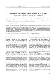
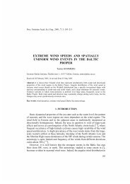
Table 4 <strong>and</strong> Fig. 4.<br />
42<br />
i=1
Table 4. Error estimate v(t max ) for Example 4<br />
J 2M v v(t max )<br />
∆t = 0.005 ∆t = 0.001<br />
4 32 0.051 0.038<br />
5 64 0.018 0.009<br />
6 128 0.0096 0.0036<br />
6<br />
4<br />
(a)<br />
u<br />
2<br />
0<br />
0 0.2 0.4 0.6 0.8 1<br />
x<br />
200<br />
100<br />
(b)<br />
a<br />
0<br />
-100<br />
-200<br />
0<br />
20 40 60 80 100 120<br />
l<br />
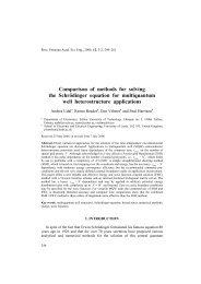
Fig. 4. Solution <strong>of</strong> <strong>the</strong> sine-Gordon equation for J = 6, ∆t = 0.001: (a) solution for <strong>the</strong><br />
instants t = 10 + 5i, i = 0, 1, 2, 3, 4; (b) <strong>wavelet</strong> coefficients at T = 30.<br />
It follows from Table 4 that already in <strong>the</strong> cases J = 4 or J = 5 we get <strong>the</strong><br />
results which visually coincide with <strong>the</strong> exact solution. The time step was taken as<br />
∆t = 0.005 or ∆t = 0.001; fur<strong>the</strong>r decrease in ∆t gave no considerable effect. If<br />
<strong>the</strong> accuracy <strong>of</strong> <strong>the</strong>se results is insufficient, more precise results could be obtained<br />
by <strong>the</strong> segmentation method proposed in [ 34 ].<br />
We would like <strong>to</strong> draw attention <strong>to</strong> Fig. 4b. It follows from here that most <strong>of</strong><br />
<strong>the</strong> <strong>wavelet</strong> coefficients are zero (or near <strong>to</strong> zero) <strong>and</strong> <strong>the</strong> number <strong>of</strong> significant<br />
coefficients is quite small. This is one <strong>of</strong> <strong>the</strong> reasons for rapid convergence <strong>of</strong> <strong>the</strong><br />
<strong>Haar</strong> <strong>wavelet</strong> series.<br />
43
6. CONCLUSIONS<br />
The main goal <strong>of</strong> this paper was <strong>to</strong> demonstrate that <strong>the</strong> <strong>Haar</strong> <strong>wavelet</strong> method<br />
is a powerful <strong>to</strong>ol for <strong>solving</strong> different types <strong>of</strong> <strong>integral</strong> equations <strong>and</strong> partial<br />
differential equations. The method with far less degrees <strong>of</strong> freedom <strong>and</strong> with<br />
smaller CPU time provides better solutions than classical ones.<br />
The main advantage <strong>of</strong> this method is its simplicity <strong>and</strong> small computation<br />
costs, resulting from <strong>the</strong> sparsity <strong>of</strong> <strong>the</strong> <strong>transform</strong> matrices <strong>and</strong> <strong>the</strong> small number <strong>of</strong><br />
significant <strong>wavelet</strong> coefficients. The method is also very convenient for <strong>solving</strong><br />
<strong>the</strong> boundary value problems, since <strong>the</strong> boundary conditions are taken care <strong>of</strong><br />
au<strong>to</strong>matically.<br />
ACKNOWLEDGEMENT<br />
Financial support from <strong>the</strong> Es<strong>to</strong>nian Science Foundation (grant No. 6697) is<br />
gratefully acknowledged.<br />
REFERENCES<br />
1. Daubechies, I. Orthonormal bases <strong>of</strong> compactly supported <strong>wavelet</strong>s. Comm. Pure Appl.<br />
Math., 1988, 41, 909–996.<br />
2. Chen, M.-Q., Hwang, C. <strong>and</strong> Shin, Y.-P. The computation <strong>of</strong> <strong>wavelet</strong>–Galerkin<br />
approximation on a bounded interval. Int. J. Numer. Methods Eng., 1996, 39, 2921–<br />
2944.<br />
3. Dahmen, W., Kurdila, A. J. <strong>and</strong> Oswald, P. (eds). Multiscale Wavelet Methods for Partial<br />
Differential Equations. Academic Press, San Diego, 1997.<br />
4. Strang, G. <strong>and</strong> Nguyen, T. Wavelets <strong>and</strong> Filter Banks. Wellesley–Cambridge Press,<br />
Wellesley (MA), 1997.<br />
5. Jameson, L. A <strong>wavelet</strong>-optimized, very much order adaptive grid <strong>and</strong> order numerical<br />
method. SIAM J. Sci. Comput., 1998, 19, 1980–2013.<br />
6. Stanković, R. S. <strong>and</strong> Falkowski, B. J. The <strong>Haar</strong> <strong>wavelet</strong> <strong>transform</strong>: its status <strong>and</strong><br />
achievements. Comput. Electr. Eng., 2003, 29, 25–44.<br />
7. Cattani, C. <strong>Haar</strong> <strong>wavelet</strong> splines. J. Interdisciplinary Math., 2001, 4, 35–47.<br />
8. Cattani, C. <strong>Haar</strong> <strong>wavelet</strong>s based technique in evolution problems. Proc. Es<strong>to</strong>nian Acad.<br />
Sci. Phys. Math., 2004, 53, 45–65.<br />
9. Chen, C. F. <strong>and</strong> Hsiao, C.-H. <strong>Haar</strong> <strong>wavelet</strong> method for <strong>solving</strong> lumped <strong>and</strong> distributedparameter<br />
systems. IEE Proc. Control Theory Appl., 1997, 144, 87–94.<br />
10. Chen, C. F. <strong>and</strong> Hsiao, C.-H. Wavelet approach <strong>to</strong> optimising dynamic systems. IEE Proc.<br />
Control Theory Appl., 1997, 146, 213–219.<br />
11. Hsiao, C.-H. <strong>and</strong> Wang, W.-J. State analysis <strong>of</strong> time-varying singular bilinear systems via<br />
<strong>Haar</strong> <strong>wavelet</strong>s. Math. Comput. Simul., 2000, 52, 11–20.<br />
12. Hsiao, C.-H. <strong>and</strong> Wang, W.-J. State analysis <strong>of</strong> time-varying singular nonlinear systems<br />
via <strong>Haar</strong> <strong>wavelet</strong>s. Math. Comput. Simul., 1999, 51, 91–100.<br />
13. Hsiao, C.-H. <strong>and</strong> Wang, W.-J. <strong>Haar</strong> <strong>wavelet</strong> approach <strong>to</strong> nonlinear stiff systems. Math.<br />
Comput. Simul., 2001, 57, 347–353.<br />
14. Hsiao, C.-H. <strong>Haar</strong> <strong>wavelet</strong> direct method for <strong>solving</strong> variational problems. Math. Comput.<br />
Simul., 2004, 64, 569–585.<br />
44
15. Hsiao, G.-C. <strong>and</strong> Rathsfeld, A. Wavelet collocation methods for a first kind boundary<br />
<strong>integral</strong> equation in acoustic scattering. Adv. Comput. Math., 2002, 17, 281–308.<br />
16. Alpert, B., Beylkin, G., Coifman, R. <strong>and</strong> Rokhlin, V. Wavelet-like bases for <strong>the</strong> fast<br />
solution <strong>of</strong> second-kind <strong>integral</strong> equations. SIAM J. Sci. Comput., 1993, 14, 159–184.<br />
17. Vainikko, G., Kivinukk, A. <strong>and</strong> Lippus, J. Fast solvers <strong>of</strong> <strong>integral</strong> equations <strong>of</strong> <strong>the</strong> second<br />
kind: <strong>wavelet</strong> methods. J. Complexity, 2005, 21, 243–273.<br />
18. Yousefi, S. <strong>and</strong> Razzaghi, M. Legendre <strong>wavelet</strong>s method for <strong>the</strong> nonlinear Volterra–<br />
Fredholm <strong>integral</strong> equations. Math. Comput. Simul., 2005, 70, 1–8.<br />
19. Maleknejad, K., Aghazadeh, N. <strong>and</strong> Molapourasl, F. Numerical solution <strong>of</strong> Fredholm<br />
<strong>integral</strong> equation <strong>of</strong> <strong>the</strong> first kind with collocation method <strong>and</strong> estimation <strong>of</strong> error<br />
bound. Appl. Math. Comput., 2006, 179, 352–359.<br />
20. Xiao, J.-Y., Wen, L.-H. <strong>and</strong> Zhang, D. Solving second kind Fredholm <strong>integral</strong> equation<br />
by periodic <strong>wavelet</strong> Galerkin method. Appl. Math. Comput., 2006, 175, 508–518.<br />
21. Kaneko, H., Noren, R. D. <strong>and</strong> Novaprateep, B. Wavelet applications <strong>to</strong> <strong>the</strong> Petrov–<br />
Galerkin method for Hammerstein equations. Appl. Numer. Math., 2003, 45, 255–273.<br />
22. Maleknejad, K. <strong>and</strong> Derili, H. The collocation method for Hammerstein equations by<br />
Daubechies <strong>wavelet</strong>s. Appl. Math. Comput., 2006, 172, 846–864.<br />
23. Avudainayagam, A. <strong>and</strong> Vano, C. Wavelet–Galerkin method for integro-differential<br />
equations. Appl. Numer. Math., 2000, 32, 247–254.<br />
24. Fedorov, M. V. <strong>and</strong> Chyev, G. N. Wavelet method for <strong>solving</strong> <strong>integral</strong> equations <strong>of</strong> simple<br />
liquids. J. Mol. Liq., 2005, 120, 159–162.<br />
25. Liang, X.-Z., Liu, M.-C. <strong>and</strong> Che, X.-J. Solving second kind <strong>integral</strong> equations by<br />
Galerkin methods with continuous orthogonal <strong>wavelet</strong>s. J. Comput. Appl. Math.,<br />
2001, 136, 149–161.<br />
26. Mahmoudi, Y. Wavelet Galerkin method for numerical solution <strong>of</strong> nonlinear <strong>integral</strong><br />
equation. Appl. Math. Comput., 2005, 167, 1119–1129.<br />
27. Khellat, F. <strong>and</strong> Yousefi, S. A. The linear Legendre mo<strong>the</strong>r <strong>wavelet</strong>s operational matrix <strong>of</strong><br />
integration <strong>and</strong> its application. J. Franklin Inst., 2006, 143, 181–190.<br />
28. Maleknejad, K. <strong>and</strong> Lotfi, T. Expansion method for linear <strong>integral</strong> equations by cardinal<br />
B-spline <strong>wavelet</strong> <strong>and</strong> Shannon <strong>wavelet</strong> bases <strong>to</strong> obtain Galerkin system. Appl. Math.<br />
Comput., 2006, 175, 347–355.<br />
29. Maleknejad, K. <strong>and</strong> Karami, M. Numerical solution <strong>of</strong> non-linear Fredholm <strong>integral</strong><br />
equations by using multi<strong>wavelet</strong>s in <strong>the</strong> Petrov–Galerkin method. Appl. Math.<br />
Comput., 2005, 168, 102–110.<br />
30. Lepik, Ü. <strong>and</strong> Tamme, E. <strong>Application</strong> <strong>of</strong> <strong>the</strong> <strong>Haar</strong> <strong>wavelet</strong>s for solution <strong>of</strong> linear <strong>integral</strong><br />
equations. In 5–10 July 2004, Antalya, Turkey – Dynamical Systems <strong>and</strong> <strong>Application</strong>s,<br />
Proceedings. 2005, 395–407.<br />
31. Lepik, Ü. <strong>and</strong> Tamme, E. Solution <strong>of</strong> nonlinear <strong>integral</strong> equations via <strong>the</strong> <strong>Haar</strong> <strong>wavelet</strong><br />
method. Proc. Es<strong>to</strong>nian Acad. Sci. Phys. Math., 2007, 56, 17–27.<br />
32. Lepik, Ü. <strong>Haar</strong> <strong>wavelet</strong> method for non-linear integro-differential equations. Appl. Math.<br />
Comput., 2006, 176, 324–333.<br />
33. Maleknejad, K. <strong>and</strong> Mirzaee, F. Using rationalized <strong>Haar</strong> <strong>wavelet</strong> for <strong>solving</strong> linear <strong>integral</strong><br />
equations. Appl. Math. Comput., 2005, 160, 579–587.<br />
34. Lepik, Ü. Numerical solution <strong>of</strong> differential equations using <strong>Haar</strong> <strong>wavelet</strong>s. Math.<br />
Comput. Simul., 2003, 68, 127–143.<br />
35. Lepik, Ü. Numerical solution <strong>of</strong> evolution equations by <strong>the</strong> <strong>Haar</strong> <strong>wavelet</strong> method. Appl.<br />
Math. Comput. (accepted).<br />
36. Newl<strong>and</strong>, D. E. An Introduction <strong>to</strong> R<strong>and</strong>om Vibrations, Spectral <strong>and</strong> Wavelet Analysis.<br />
Longman Scientific <strong>and</strong> Technical, New York, 1993.<br />
37. Kim, B. H., Kim, H. <strong>and</strong> Park, T. Nondestructive damage evaluation <strong>of</strong> plates using <strong>the</strong><br />
multiresolution analysis <strong>of</strong> two-dimensional <strong>Haar</strong> <strong>wavelet</strong>. J. Sound Vibration, 2006,<br />
292, 82–104.<br />
45
38. Kumar , B. V. R. <strong>and</strong> Mehra, M. Wavelet based preconditioners for sparse linear systems.<br />
Appl. Math. Comput., 2005, 171, 203–224.<br />
39. Cattani, C. Wavelet analysis <strong>of</strong> dynamical systems. Electron. Commun. (Kiev), 2002, 17,<br />
115–124.<br />
40. Forinash, K. <strong>and</strong> Willis, C. R. Nonlinear response <strong>of</strong> <strong>the</strong> sine-Gordon brea<strong>the</strong>r <strong>to</strong> an a.c.<br />
driver. Physica D, 2001, 149, 95–106.<br />
<strong>Haar</strong>i lainikute rakendamine integraalja<br />
diferentsiaalvõrr<strong>and</strong>ite lahendamiseks<br />
Ülo Lepik<br />
Oma lihtsuse tõttu on <strong>Haar</strong>i lainikud leidnud järjest enam rakendusvõimalusi.<br />
Muuhulgas on need osutunud väga efektiivseteks diferentsiaal- ja integraalvõrr<strong>and</strong>ite<br />
lahendamisel. Artiklis, mis suures osas baseerub au<strong>to</strong>ri uurimustel, on<br />
püütud <strong>and</strong>a ülevaade probleemi tänapäevasest seisundist.<br />
Tulemuste täpsuse hindamiseks on lahendatud hulk üles<strong>and</strong>eid, mille puhul<br />
on täpne lahend teada. Neist näidetest selgub, et <strong>Haar</strong>i mee<strong>to</strong>d on klassikaliste<br />
lahendusviisidega täiesti konkurentsivõimeline. Eelisteks on aga mee<strong>to</strong>di lihtsus,<br />
universaalsus, väike võrgupunktide arv ja lühike arvutiaeg.<br />
46