LECTURE 4: Numerical integration

1
LECTURE 4: Numerical integration
October 9, 2012
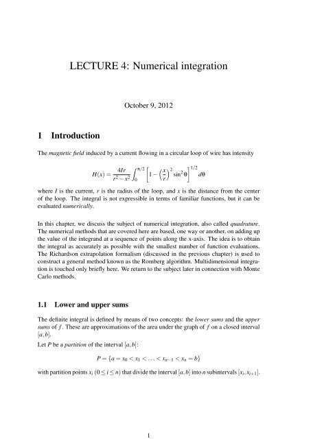
1 Introduction
The magnetic field induced by a current flowing in a circular loop of wire has intensity
H(x) =
4Ir ∫ π/2
[ ( x
) ] 2 1/2
r 2 − x 2 1 − sin 2 θ dθ
0 r
where I is the current, r is the radius of the loop, and x is the distance from the center
of the loop. The integral is not expressible in terms of familiar functions, but it can be
evaluated numerically.
In this chapter, we discuss the subject of numerical integration, also called quadrature.
The numerical methods that are covered here are based, one way or another, on adding up
the value of the integrand at a sequence of points along the x-axis. The idea is to obtain
the integral as accurately as possible with the smallest number of function evaluations.
The Richardson extrapolation formalism (discussed in the previous chapter) is used to
construct a general method known as the Romberg algorithm. Multidimensional integration
is touched only briefly here. We return to the subject later in connection with Monte
Carlo methods.
1.1 Lower and upper sums
The definite integral is defined by means of two concepts: the lower sums and the upper
sums of f . These are approximations of the area under the graph of f on a closed interval
[a,b].
Let P be a partition of the interval [a,b]:
P = {a = x 0 < x 1 < ... < x n−1 < x n = b}
with partition points x i (0 ≤ i ≤ n) that divide the interval [a,b] into n subintervals [x i ,x i+1 ].

2
Denote by m i the greatest lower bound (infimum) of f (x) on [x i ,x i+1 ]:
m i = inf{ f (x) : x i ≤ x ≤ x i+1 }
Likewise, denote by M i the least upper bound (supremum) of f (x) on [x i ,x i+1 ]:
M i = sup{ f (x) : x i ≤ x ≤ x i+1 }
The lower sums and upper sums of f corresponding to a given partition P are defined to
be
L( f ;P) =
U( f ;P) =
n−1
∑
i=0
m i (x i+1 − x i )
n−1
∑ M i (x i+1 − x i )
i=0
If f is positive, then these two quantities can be interpreted as estimates of the area under
the curve for f .
a=x0 x1 x2 x3 x4 x5 x6 x7 x8=b
Figure 1: Lower sums.
a=x0 x1 x2 x3 x4 x5 x6 x7 x8=b
Figure 2: Upper sums.

3
1.2 Riemann-integrable functions
Consider the least upper bound obtained when P is allowed to range over all partitions of
the interval [a,b]. This is abbreviated sup P L( f ;P). Similarly, the greatest lower bound,
when P ranges over all partitions P on [a,b], is abbreviated inf P L( f ;P).
If these two numbers are the same,
sup
P
then f is Riemann integrable on [a,b].
L( f ;P) = infL( f ;P)
P
Theorem. Every continuous function defined on a closed interval of the real line is Riemann
integrable.
The Riemann integral of a continuous function on [a,b] can be obtained by two limits:
lim sup
n→∞ P
L( f ;P n ) =
∫ b
a
f (x)dx = lim
n→∞
inf
P L( f ;P n)
Here the length of the largest subinterval in P n converges to zero as n → ∞.
Direct translation of this definition into a numerical algorithm is possible, but the resulting
algorithm converges very slowly. The situation can be improved dramatically by using
more sophisticated methods such as the Romberg’s algorithm.

4
2 Trapezoid rule
The trapezoid method is based on an estimation of the area under a curve using trapezoids.
First the interval [a,b] is divided into subintervals according to the partition P =
{a = x 0 < x 1 < ... < x n−1 < x n = b}.
A typical trapezoid has the subinterval [x i ,x i+1 ] as its base, and the two vertical sides are
f (x i ) and f (x i+1 ). The area is equal to the base times the average height. Thus we obtain
the basic trapezoid rule:
∫ xi+1
x i
f (x)dx ≈ A i = 1 2 (x i+1 − x i )[ f (x i ) + f (x i+1 )]
The total area under all of the trapezoids is given by the composite trapezoid rule:
∫ b
a
f (x)dx ≈ T ( f ;P) =
n−1
∑
i=0
A i = 1 2
n−1
∑
i=0
(x i+1 − x i )[ f (x i ) + f (x i+1 )]
f(xi)
f(xi+1)
xi
xi+1
Figure 3: The basic trapezoid rule.
2.1 Uniform spacing
In practice, the trapezoid rule is used with uniform partition of the interval. The division
points x i are equally spaced: x i = a + ih, where h = (b − a)/n and 0 ≤ i ≤ n. This gives a
simpler formula
∫ b
a
f (x)dx ≈ T ( f ;P) = h 2
n−1
∑
i=0
[ f (x i ) + f (x i+1 )]
A computationally preferable form is written as
{ }
∫ b
n−1
f (x)dx ≈ T ( f ;P) = h ∑ f (x i ) + 1
a
i=1
2 [ f (x 0) + f (x n )]

5
Implementation
The following procedure Trapezoid uses the trapezoid method with uniform spacing to
estimate the definite integral of a function f on a closed interval [a,b].
double Trapezoid(double (*f)(double x),
double a, double b, int n)
{
int i;
double h, result;
h = (b-a)/(double)n;
result = 0.5*(f(a)+f(b));
for(i=1; i

6
2.2 Error analysis
Theorem on precision of trapezoid rule.
If f ′′ exists and is continuous on the interval [a,b], and if the composite trapezoid rule T
with uniform spacing h is used to estimate the integral I = ∫ b
a f (x)dx, then for some ξ in
(a,b),
I − T = − 1
12 (b − a)h2 f ′′ (ξ) = O(h 2 )
To prove this use the error formula for polynomial interpolation with n = 1, x 0 = 0, and
x 1 = 1: f (x)− p(x) = 1
(n+1)! f (n+1) (ξ)∏ n i=0 (x−x i) plus mean-value theorem ∫ b
a f (x)g(x)dx =
f (ξ) ∫ b
a g(x)dx. Example. If the trapezoid rule is used to compute
I =
∫ 1
0
e −x2 dx
with an error at most 1 2 × 10−4 , how many points should be used?
The error formula is
In this example,
f (x) = e −x2
f ′ (x) = −2xe −x2
f ′′ (x) = (4x 2 − 2)e −x2
I − T = − 1 12 (b − a)h2 f ′′ (ξ)
Thus, | f ′′ (x)| ≤ 2 on the interval [0,1], and
|I − T | ≤ 1 6 h2
To have an error of at most 1 2 × 10−4 , we require that h = (b − a)/n ≤ 0.01732 or n ≥ 58.
Using the procedure Trapezoid with n = 58, we obtain 0.7468059 which is incorrect in
the fifth digit.

7
2.3 Recursive trapezoid formula
We now introduce a formula for the composite trapezoid rule when the interval [a,b] is
subdivided into 2 n equal parts. We have
n−1
T ( f ;P) = h ∑
= h
i=1
n−1
∑
i=1
f (x i ) + h 2 [ f (x 0) + f (x n )]
f (a + ih) + h [ f (a) + f (b)]
2
If we now replace n by 2 n and use h = (b − a)/2 n , the formula becomes
2 n −1
R(n,0) = h ∑ f (a + ih) + h [ f (a) + f (b)]
i=1
2
Here we have introduced the notation R(n,0) which is used in the next section in connection
with the Romberg algorithm. The notation R(n,0) denotes the result of applying the
composite trapezoid rule with 2 n equal subintervals.
SUBINTERVALS
0
2
2
2
1
2
a
ARRAY
R(0,0)
R(1,0)
R(2,0)
R(3,0)
b
2 3 Figure 5: The recursive trapezoid rule.
For the Romberg algorithm, we need a method for computing R(n,0) from R(n − 1,0)
without unnecessary evaluations of f . We use the identity
R(n,0) = 1 2 R(n − 1,0) + [R(n,0) − 1 R(n − 1,0)]
2
It is desirable to compute the bracketed expression with as little extra computation as
possible. We have
2 n −1
R(n,0) = h ∑ f (a + ih) +C
i=1
2 n−1 −1
R(n − 1,0) = 2h ∑ f (a + 2 jh) + 2C
j=1
where
C = h [ f (a) + f (b)]
2
Notice that the size of the subintervals for R(n − 1,0) are twice the size of those for
R(n,0).

8
By subtraction we get
R(n,0) − 1 2 R(n − 1,0) = h 2 n −1
∑
i=1
2 n−1 −1
f (a + ih) − h ∑ f (a + 2 jh)
j=1
2 n−1
= h ∑ f [a + (2k − 1)h]
k=1
Here we have taken into account that each term in the first sum that corresponds to an even
value of i is canceled by a term in the second sum. This leaves only terms that correspond
to odd values of i.
This gives us the recursive trapezoid formula.
If R(n − 1,0) is available, then R(n,0) can be computed by the formula
R(n,0) = 1 2 n−1
2 R(n − 1,0) + h ∑ f [a + (2k − 1)h] (n ≥ 1)
k=1
using h = (b − a)/2 n and R(0,0) =
2 1 (b − a)[ f (a) + f (b)].
Implementation
The following procedure RecTrapezoid uses the recursive trapezoid formula to calculate
a sequence of approximations to the definite integral of function f on the interval [a,b].
void RecTrapezoid(REAL (*f)(REAL x), REAL a, REAL b,
int n, REAL *R)
{
int i, j, k, kmax=1;
REAL h, sum;
}
h = b-a;
/* Value of R(0,0) */
R[0] = (h/2.0)*(f(a)+f(b));
/* Successive approximations R(n,0) */
for(i=1; i

9
Example.
The procedure RecTrapezoid was used to calculate the value of π by evaluating the integral
π ≈
∫ 1
The following output is obtained with n = 9:
R(0,0) = 3.000000000000
R(1,0) = 3.100000000000
R(2,0) = 3.131176470588
R(3,0) = 3.138988494491
R(4,0) = 3.140941612041
R(5,0) = 3.141429893175
R(6,0) = 3.141551963486
R(7,0) = 3.141582481064
R(8,0) = 3.141590110458
R(9,0) = 3.141592017807
0
4
1 + x 2 dx
The approximation is correct in the sixth decimal. The correct value is 3.141592654 with
nine decimals.
Next, we introduce the Romberg algorithm which uses the numbers R(n,0) and improves
the estimates in a fashion similar to that of Richardson extrapolation.

10
3 Romberg algorithm
3.1 Description
The Romberg algorithm produces a triangular array of numbers, all of which are numerical
estimates of the definite integral ∫ b
a f (x)dx. The array is denoted by
R(0,0)
R(1,0) R(1,1)
R(2,0) R(2,1) R(2,2)
R(3,0) R(3,1) R(3,2) R(3,3)
. . . .
R(n,0) R(n,1) R(n,2) R(n,3) ... R(n,n)
The first column contains estimates R(k,0) obtained by applying the trapezoid rule with
2 k equal subintervals. The first one is obtained using the formula
R(0,0) = 1 (b − a)[ f (a) + f (b)]
2
R(n,0) is obtained easily from R(n − 1,0) using the formula developed in the previous
section:
R(n,0) = 1 2 n−1
2 R(n − 1,0) + h ∑ f [a + (2k − 1)h]
k=1
where h = (b − a)/2 n and n ≥ 1.
The second and successive columns are generated by the following extrapolation formula:
R(n,m) = R(n,m − 1) + 1
4 m [R(n,m − 1) − R(n − 1,m − 1)]
− 1
with n ≥ 1 and m ≥ 1. This formula results from the application of the Richardson extrapolation
theorem.

11
3.2 Derivation of the Romberg algorithm
To briefly sketch where the iterative equation behind Romberg algorithm comes from we
start from the following formula where the error is expressed in the trapezoid rule with
2 n−1 equal subintervals
∫ b
a
f (x)dx = R(n − 1,0) + a 2 h 2 + a 4 h 4 + a 6 h 6 + ...
This is one form of Euler-Maclaurin formula (see the next page). (A proof can be found
for instance in Gregory, R.T, and Kearney, D., A Collection of Matrices for Testing Computational
Algorithms (Wiley, 1969).) Here h = (b − a)/2 n and the coefficients a i depend
on f but not on h. R(n − 1,0) is one of the trapezoidal elements in the Romberg array.
For our purposes, it is not necessary to know the definite expressions for the coefficients.
For the theory to work smoothly, we assume that f possesses derivatives of all orders on
the interval [a,b].
Now recall the theory of Richardson extrapolation. We can use the same procedure here
due to the form of the equation above. Replacing n with n + 1 and h with h/2, we have
∫ b
a
f (x)dx = R(n,0) + 1 4 a 2h 2 + 1
16 a 4h 4 + 1
64 a 6h 6 + ...
Subtracting the first equation from the second equation multiplied by 4 gives
where
∫ b
a
f (x)dx = R(n,1) − 1 4 a 4h 4 − 5
16 a 6h 6 − ...
R(n,1) = R(n,0) + 1 [R(n,0) − R(n − 1,0)] (n ≥ 1)
3
Note that this is the first case (m = 1) of the extrapolation formula that is used to generate
the Romberg array.
The term R(n,1) should be considerably more accurate than R(n,0) or R(n − 1,0) since
the error series is now O(h 4 ). This process can be repeated to further eliminate higher
terms in the error series.
The only assumption made is that the first equation with the error series is valid for the
function f . In practice, we use only a modest number of rows in the Romberg algorithm,
which means that the assumption is likely to be valid. The situation is governed by a
theorem called the Euler-Maclaurin formula.

12
3.3 Euler-Maclaurin formula and error term
Theorem.
If f (2m) exists and is continuous on the interval [a,b], then
∫ b
a
f (x)dx = h 2
n−1
∑
i=0
where h = (b − a)/n, x i = a + ih for 0 ≤ i ≤ n, and
E =
for some ξ in the interval (a,b).
[ f (x i ) + f (x i+1 )] + E
m−1
∑ A 2k h 2k [ f (2k−1) (a) − f (2k−1) (b)] − A 2m (b − a)h 2m f (2m) (ξ)
k=1
In this theorem, the A k ’s are constants and they can be defined by the equation (see
e.g. D.M. Young and R.T. Gregory, A survey of Numerical Mathematics, Vol.1, p. 374,
(Dover) for details):
∞
x
e x − 1 = ∑ A k x k
k=0
The points to notice are that the right-hand side of the Euler-Maclaurin formula contains
the trapezoid rule and an error term E. Furthermore, the error term can be expressed as a
finite sum in ascending powers of h 2 .
This theorem gives the formal justification to the Romberg algorithm.

13
3.4 Implementation
The following procedure Romberg uses the extrapolation formula to calculate numerical
estimates of the definite integral ∫ b
a f (x)dx. The input is the function f , the endpoints of
the interval [a,b], the number of iterations n and the Romberg array (R) 0:n×0:n .
void Romberg(double (*f)(double x),
double a, double b, int n,
double R[][MAXN])
{
int i, j, k, kmax=1;
double h, sum;
h = b-a;
R[0][0] = (h/2.0)*(f(a)+f(b));
for(i=1; i

14
Output
Using same example as before, we calculate the value of π by evaluating the integral
(Correct value is 3.141592654.)
π ≈
∫ 1
0
4
1 + x 2 dx
The output using double-precision:
3.0000000000
3.1000000000 3.1333333333
3.1311764706 3.1415686275 3.1421176471
3.1389884945 3.1415925025 3.1415940941 3.1415857838
3.1409416120 3.1415926512 3.1415926611 3.1415926384 3.1415926653
3.1414298932 3.1415926536 3.1415926537 3.1415926536 3.1415926536 3.1415926536
And using single-precision:
3.0000000000
3.0999999046 3.1333332062
3.1311764717 3.1415686607 3.1421177387
3.1389884949 3.1415925026 3.1415941715 3.1415858269
3.1409416199 3.1415927410 3.1415927410 3.1415927410 3.1415927410
3.1414299011 3.1415927410 3.1415927410 3.1415927410 3.1415927410 3.1415927410
We notice that the algorithm converges very quickly (with double precision, n = 5 is
enough to obtain nine decimals of precision). With single precision, the accuracy of the
calculation is limited to six decimals.

15
4 Adaptive Simpson’s scheme
We now proceed to discussing a method known as the Simpson’s rule and develop an
adaptive scheme for obtaining a numerical approximation for the integral ∫ b
a f (x)dx. In
the adaptive algorithm, the partitioning of the interval [a,b] is not selected beforehand but
automatically determined.
4.1 Simpson’s rule
A considerable improvement over the trapezoid rule can be achieved by approximating
the function within each of the n subintervals by some polynomial. When second-order
polynomials are used, the resulting algorithm is called the Simpson’s rule.
Dividing the interval [a,b] into two equal subintervals with partition points a, a + h and
a + 2h = b results in the basic Simpson’s rule:
∫ a+2h
a
f (x)dx ≈ h [ f (a) + 4 f (a + h) + f (a + 2h)]
3
Proof. Approximating the function with a polynomial of degree ≤ 2 we can write ∫ b
a f (x)dx ≈
A f (a) + B f ( a+b
2
) +C f (b), where f (x) is assumed continuous on the interval [a,b]. The
coefficients A, B and C are chosen such that the approximation will give correct values
for the integral when f is aquadratic polynomial. Let a = −1 and b = 1: ∫ 1
−1 f (x)dx ≈
A f (−1) + B f (0) +C f (1). The following equations must hold:
f (x) = 1 : ∫ 1
−1 dx = 2 = A + B +C
f (x) = x : ∫ 1
−1 xdx = 0 = −A +C
f (x) = x 2 : ∫ 1
−1 x 2 dx = 2/3 = A +C
⇒ A = 1/3, B = 4/3, and C = 1/3. ⇒ ∫ 1
−1 f (x)dx ≈ 1 3
[ f (−1) + 4 f (0) + f (1)]. Using
the linear mapping y = (b − a)/2 + (a + b)/2 from [−1,1] to [a,b] we obtain the basic
Simpson’s rule: ∫ b
a f (x)dx ≈ 1 a+b
6
(b − a)[ f (a) + 4 f (
2 ) + f (b)].
The error can be estimated using Taylor series:
f (a + h) = f + h f ′ + 1 2! h2 f ′′ + 1 3! h3 f ′′′ + ...
f (a + 2h) = f + 2h f ′ + 2h 2 f ′′ + 4 3 h3 f ′′′ + ...
From these we obtain a series representation for the right-hand side of the Simpson’s rule:
h
3 [ f (a) + 4 f (a + h) + f (a + 2h)] = 2h f + 2h2 f ′ + 4 3 h3 f ′′ + 2 3 h4 f ′′′ + ...(∗)
Now consider the left-hand side.
∫ a+2h
with
a
f (x)dx = F(a + 2h) − F(a)
F(x) =
Thus, F ′ = f , F ′′ = f ′ , F ′′′ = f ′′ and so on.
∫ x
a
f (t)dt

16
Now use the Taylor series for F(a + 2h):
F(a + 2h) = F(a) + 2hF ′ (a) + 2h 2 F ′′ (a) + 4 3 h3 F ′′′ (a) + ...
= F(a) + 2h f (a) + 2h 2 f ′ (a) + 4 3 h3 f ′′ (a) + ...(∗∗)
F(a) = 0, so F(a + 2h) = ∫ a+2h
a f (x)dx.
Subtracting (**) from (*) gives us an estimate of the error:
∫ a+2h
f (x)dx − h h5
[ f (a) + 4 f (a + h) + f (a + 2h)] = −
3 90 f (4) − ...
a
This is due to the fact that all lower order terms cancel out.
So, the basic Simpson’s rule over the interval [a,b] is
∫ b
( )
(b − a)
a + b
f (x)dx ≈ [ f (a) + 4 f + f (b)]
6
2
with the error term
a
− 1
90
which is O(h 5 ) for some ξ in (a,b).
( ) b − a 5
f (4) (ξ)
2
4.2 Adaptive Simpson’s algorithm
In the adaptive process, the interval [a,b] is first divided into two subintervals. Then we
decide whether each of the two subintervals is further divided into more subintervals. The
process continues until some specified accuracy is reached.
We now develop the test for deciding whether subintervals should continue to be divided.
The Simpson’s rule over the interval [a,b] can be written as
I ≡
∫ b
where S is given by the basic Simpson’s rule
and E is the error term
S(a,b) =
a
f (x)dx = S(a,b) + E(a,b)
(b − a)
[ f (a) + 4 f
6
E(a,b) = − 1
90
( a + b
2
( ) b − a 5
f (4) (ξ)
2
)
+ f (b)]
We assume here that f (4) remains constant throughout the interval [a,b]. Letting h = b−a,
we have
I = S (1) + E (1)
where
S (1) = S(a,b) and E (1) = − 1 ( ) h 5
f (4)
90 2

17
Two applications of the Simpson’s rule give
where
and
Here c = (a + b)/2.
E (2) = − 1
90
( h/2
I = S (2) + E (2)
S (2) = S(a,c) + S(c,b)
2
) 5
f (4) − 1
90
( ) h/2 5
f (4) = 1 16 E(1)
2
We can now subtract the first evaluation from the second one:
I − I = 0 = S (2) + E (2) − S (1) − E (1)
S (2) − S (1) = E (1) − E (2) = 15E (2)
E (2) = 1
15 (S(2) − S (1) )
We can now write the second application of the Simpson’s rule as
I = S (2) + E (2) = S (2) + 1
15 (S(2) − S (1) )
This can be used to evaluate the quality of our approximation of I. We can use the following
inequality to test whether to continue the splitting process:
1
15 |S(2) − S (1) | < ε
If the test is not satisfied, the interval [a,b] is split into two subintervals [a,c] and [c,b].
On each of these subintervals we perform the test again with ε replaced by ε/2 so that the
resulting tolerance will be ε over the entire interval [a,b].

18
4.3 Algorithm
The adaptive Simpson’s algorithm is programmed using a recursive procedure.
We define two variables one_simpson and two_simpson that are used to calculate
two Simpson approximations: one with two subintervals another with four half-width
subintervals.
one_simpson is given by the basic Simpson’s rule:
S (1) = S(a,b) = h [ f (a) + 4 f (c) + f (b)]
6
two_simpson is given by two Simpson’s rules:
S (2) = S(a,c) + S(c,b) = h [ f (a) + 4 f (d) + 2 f (c) + 4 f (e) + f (b)]
12
One Simpson’s rule
a
c
b
Two Simpson’s rules
a
d c
e b
h/2 h/2
Figure 6: Simpson’s rules used in the adaptive algorithm.
After evaluating S (1) and S (2) , we use the division test
1
15 |S(2) − S (1) | < ε
to check whether to divide the subintervals further.
If the criterion is not fulfilled, the procedure calls itself with left_simpson corresponding
to the left side [a,c] and right_simpson corresponding to the right side
[c,b]. At each recursive call, the value of ε is divided in half. Variable level keeps
track of the level of the current interval division. The maximum allowed level is given by
level_max.
The final estimate for each subinterval is given by the Two Simpson’s rules (when the
criterion is fulfilled). At each upper level, the answer is given by the sum of the left side
and the right side.

19
Implementation
The following C implementation of the recursive procedure Simpson calculates the definite
integral ∫ b
a f (x)dx for the function f specified by an external function f (given as
input).
double Simpson(double a, double b, double eps,
int level, int level_max)
{
int i, j, k, kmax=1;
double c, d, e, h, result;
double one_simpson, two_simpson;
double left_simpson, right_simpson;
h = b-a;
c = 0.5*(a+b);
one_simpson = h*(f(a)+4.0*f(c)+f(b))/6.0;
d = 0.5*(a+c);
e = 0.5*(c+b);
two_simpson = h*(f(a)+4.0*f(d)+2.0*f(c)+4.0*f(e)+f(b))/12.0;
/* Check for level */
if(level+1 >= level_max) {
result = two_simpson;
printf("Maximum level reached\n");
}
else{
/* Check for desired accuracy */
if(fabs(two_simpson-one_simpson) < 15.0*eps)
result = two_simpson + (two_simpson-one_simpson)/15.0;
/* Divide further */
else {
left_simpson = Simpson(a,c,eps/2.0,level+1,level_max);
right_simpson = Simpson(c,b,eps/2.0,level+1,level_max);
result = left_simpson + right_simpson;
}
}
return(result);
}

20
Application example
As an example, the program is used to calculate the integral
∫ 2π
[ ] cos(2x)
e x dx
0
The desired accuracy is set to ε = 1 2 ×10−4 . An external function procedure is written for
f and its name is given as the first argument to Simpson.
Running the program with double precision floating-point numbers, we obtain the result
0.1996271. It is correct within the tolerance we set beforehand.
We can use Matlab or Maple to determine the correct answer. The following Matlab
commands
syms t
res = int(cos(2*t)./exp(t),0,2*pi)
eval(res)
first return the exact value 1 5 (1 − e−2π ) and then evaluate the integral giving (with ten
digits) 0.19962 65115.

21
5 Gaussian quadrature formulas
We have already seen that the various numerical integration formulas all have the common
feature that the integral is approximated by the sum of its functional values at a set of
points, multiplied by certain aptly chosen weighting coefficients. We have seen that by
a better selection of the weights, we can gain integration formulas of higher and higher
order. The idea of Gaussian quadrature formulas is to give ourselves the freedom to
choose not only the weighing factors but also the points where the function values are
calculated. They will no longer be equally spaced.
Now the catch: high order is not the same as high accuracy! High order translates to high
accuracy only when the integrand is very smooth, in the sense of being well-approximated
by a polynomial.
5.1 Description
Most numerical integration formulas conform to the following pattern:
∫ b
a
f (x)dx ≈ A 0 f (x 0 ) + A 1 f (x 1 ) + ... + A n f (x n )
To use such a formula, it is only necessary to know the nodes x 0 ,x 1 ,...,x n and the weights
A 0 ,A 1 ,...,A n .
The theory of polynomial interpolation has greatly influenced the development of integration
formulas. If the nodes have been fixed, there is a corresponding Lagrange interpolation
formula:
p n (x) =
n
∑
i=0
l i (x) f (x i ) where l i (x) =
n
∏
j=0
j≠i
( ) x − x j
x i − x j
This formula provides a polynomial p that interpolates f at the nodes. If circumstances
are favorable, p will be a good approximation to f , and also
∫ b
a
f (x)dx ≈
∫ b
a
p(x)dx =
n ∫ b
∑ f (x i ) l i (x)dx =
i=0 a
n
∑
i=0
A i f (x i )
where
A i =
∫ b
a
l i (x)dx

22
Example.
Determine the quadrature formula when the interval is [−2,2] and the nodes are -1, 0 and
1.
Solution. The cardinal functions are given by
l i (x) =
n
∏
j=0
j≠i
( ) x − x j
x i − x j
We get l 0 (x) =
2 1x(x − 1), l 1(x) = −(x + 1)(x − 1) and l 2 (x) = 1 2x(x + 1).
The weights are obtained by integrating these functions. For example
A 0 =
∫ 2
−2
Similarly, A 1 = −4/3 and A 2 = 8/3.
l 0 (x)dx = 1 2
∫ 2
−2(x 2 − x)dx = 8 3
The quadrature formula is
∫ 2
−2
f (x)dx ≈ 8 3 f (−1) − 4 3 f (0) + 8 3 f (1)

23
5.2 Gaussian nodes and weights
The mathematician Karl Friedrich Gauss (1777-1855) discovered that by a special placement
of the nodes the accuracy of the numerical integration process could be greatly
increased.
Gaussian quadrature theorem.
Let q be a nontrivial polynomial of degree n + 1 such that
∫ b
a
x k q(x)dx = 0 (0 ≤ k ≤ n)
Let x 0 ,x 1 ,...,x n be the zeros of q. The formula
∫ b
a
f (x)dx ≈
n
∑
i=0
A i f (x i ) where A i =
∫ b
a
l i (x)dx
(∗)
with these x i ’s as nodes will be exact for all polynomials of degree at most 2n + 1. Furthermore,
the nodes lie in the open interval (a,b).
To summarize: With arbitrary nodes, the equation (*) is exact for all polynomials of degree
≤ n. With the Gaussian nodes, the equation (*) is exact for all polynomials of degree
≤ 2n + 1.
The quadrature formulas that arise as applications of this theorem are called Gaussian or
Gauss-Legendre quadrature formulas.

24
Example
As an example, we derive a Gaussian quadrature formula that is not too complicated.
We determine the formula with three Gaussian nodes and three weights for the integral
∫ 1−1
f (x)dx.
We must find the polynomial q and compute its roots. The degree of q is 3, so it has the
form
q(x) = c 0 + c 1 x + c 2 x 2 + c 3 x 3
The conditions that q must satisfy are
∫ 1
−1
q(x)dx =
∫ 1
−1
xq(x)dx =
∫ 1
−1
x 2 q(x)dx = 0
If we let c 0 = c 2 = 0, then q(x) = c 1 x + c 3 x 3 . The integral of an odd function over a
symmetric interval is 0 and so we have
∫ 1
−1
q(x)dx =
∫ 1
To obtain c 1 and c 3 , we impose the condition
∫ 1
−1
−1
x 2 q(x)dx = 0
x(c 1 x + c 3 x 3 )dx = 0
A convenient solution of this is c 1 = −3 and c 3 = 5. Hence
q(x) = 5x 3 − 3x
The roots are 0 and ± √ 3/5. These are the desired Gaussian nodes for the quadrature
formula.
To obtain the weights A 0 , A 1 and A 2 , we use a procedure known as the method of undetermined
coefficients. Consider the formula
( √ (√
3 3
5)
5)
∫ 1
−1
f (x)dx ≈ A 0 f
−
+ A 1 f (0) + A 2 f
We want to select the coefficients A i in such a way that the approximate equality (≈) is an
exact equality (=) whenever f is of the form ax 2 + bx + c.

25
Since integration is a linear process, the above formula will be exact for all polynomials
of degree ≤ 2 if the formula is exact for 1, x and x 2 . In tabular form
f left-hand side right-hand side
∫
1 1−1
dx = 2 A 0 + A 1 + A 2
∫
√ √
x 1−1 3
xdx = 0 −
5 A 3
0 +
5 A 2
x 2 ∫ 1−1
x 2 dx =
3
2 3
5 A 0 + 3 5 A 2
Thus we get ⎧
⎪⎨
⎪ ⎩
A 0 + A 1 +A 2 = 2
A 0 −A 2 = 0
A 0 +A 2 = 10/9
The weights are A 0 = A 2 = 5/9 and A 1 = 8/9.
Therefore, the final formula is
∫ 1
−1
f (x)dx ≈ 5 9 f (−
√ )
3
5)
+ 8 9 f (0) + 5 9 f (√
3
5
This will integrate all polynomial of degree 4 or less correctly.
For example, ∫ 1
−1 x 4 dx = 2/5. The formula yields the same value.
Example 2 - Application to a nonpolynomial
With the transformation t = [2x−(b+a)]/(b−a), a Gaussian quadrature rule of the form
∫ 1
−1
f (t)dt ≈
n
∑
i=0
A i f (t i )
can be used over an arbitrary interval [a,b]. The substitution gives
∫ b
f (x)dx = 1 ∫ 1
[ 1
2 (b − a) f
2 (b − a)t + 1 ]
2 (b + a) dt
a
−1
We can now use the obtained formula
∫ 1
−1
f (x)dx ≈ 5 9 f (−
and the transformation to approximate the integral
√ )
3
5)
∫ 1
0
e −x2 dx
+ 8 9 f (0) + 5 9 f (√
3
5

26
We have
∫ 1
0
f (x)dx = 1 ∫ 1
( 1
f
2 −1 2 t + 1 dt
2)
[ ( )
≈ 1 5
2 9 f 1
2 2√ − 1 3
+ 8 ( ) ( )]
1
5 9 f + 5 2 9 f 1
2 + 1 3
2√
5
Letting f (x) = e −x2 , we get
∫ 1
0
e −x2 dx ≈ 0.746814584
The true solution is
2 1 erf(1) ≈ 0.7468241330. Thus the error in the approximation given
by the quadrature formula is of the order 10 −5 . This is excellent, considering that only
three function evaluations were made!
5.3 Tables of nodes and weights
The numerical values of nodes and weights for several values of n have been tabulated
and can be found in references.
Table 5.1 in Cheney and Kincaid gives the values for n ≤ 4. They can be applied for the
Gaussian quadrature formula
∫ b
a
f (x)dx ≈
n
∑
i=0
A i f (x i )
As an example, the case for n = 2 was discussed in the previous example; i.e. for x i =
− √ 3/5,0, √ 3/5 and A i = 5/9,8/9,5/9.

27
5.4 Multidimensional integration
In general, multidimensional integration is more difficult and computationally much more
time consuming than evaluating one-dimensional integrals. The subject is discussed only
briefly here. We return to the subject later on in connection with Monte Carlo methods.
If the area of integration is relatively simple and the integrand is smooth, we can use a
sequence of one-dimensional integrals:
∫∫∫
∫ x2
∫ y2 (x) ∫ z2 (x,y)
I = f (x,y,z)dxdydz = dx dy dz f (x,y,z)
y 1 (x) z 1 (x,y)
Denote the innermost integral by G(x,y):
G(x,y) =
and the integral of this function by H(x):
The final result is given by
H(x) =
I =
x 1
∫ z2 (x,y)
z 1 (x,y)
∫ y2 (x)
y 1 (x)
∫ x2
x 1
f (x,y,z)dz
G(x,y)dy
H(x)dx
For simplicity, we illustrate with the trapezoid rule for the interval [0,1], using n + 1
equally spaced points. The step size is therefore h = 1/n. The composite trapezoid rule is
∫ 1
We write this in the form ∫ 1
f (x)dx ≈
0
f (x)dx ≈ 1
n−1
2h [ f (0) + 2 ∑ f ( i
i=1
n ) + f (1)]
0
n
∑
i=0
A i f ( i n )
The error is O(h 2 ) = O(n −2 ) for functions having a continuous second derivative.
If we now want to evaluate a two-dimensional integral over the unit square, we can
apply the trapezoid rule twice:
∫ 1 ∫ 1
0
0
f (x,y)dxdy ≈
=
≈
=
∫ 1 n
∑
0 i=0
n ∫ 1
∑ A i
i=0 0
n n
∑ i ∑
i=0A
j=0
n
∑
i=0
A i f ( i n ,y)dy
f ( i n ,y)dy
A j f ( i n , j n )
n
∑ A i A j f ( i
j=0
n , j n )
The error is again O(h 2 ) because each of the two applications of the trapezoid rule entails
this error.

28
In the same way, we can integrate a function of k variables. The trapezoid rule in the
general case for integration over the multidimensional unit hypercube is given by
∫
[0,1] k f (x)dx ≈ n
∑
α 1 =0
...
n
∑
α k =0
A α1 ...A αk f ( α 1
n ,..., α k
n )
Now consider the computational effort that is required for evaluating the integrals using
the trapezoid rule. In the one-dimensional case, the work involved is O(n). In the twovariable
case, it is O(n 2 ), and O(n k ) for k variables.
Thus for a constant number of nodes (constant effort) the quality of the numerical approximation
to the value of the integrals declines very quickly as the number of variables
increases. This explains why the Monte Carlo methods for numerical integration become
an attractive option for high-dimensional integration.
Example.
In order to evaluate the integral of f (x,y) = xye −x2y over the square x,y ∈ [0,1], we can
modify the procedure Trapezoid to obtain a two-dimensional version:
double Trapezoid_2D(double (*f)(double x,double y),
double ax, double bx,
double ay, double by, int n)
{
int i, j;
double hx, hy, result;
hx = (bx-ax)/(double)n;
hy = (by-ay)/(double)n;
result = 0.5*(f(ax,ay)+f(bx,by));
for(i=1; i