Semi-Supervised Classification via Local Spline Regression
Semi-Supervised Classification via Local Spline Regression
Semi-Supervised Classification via Local Spline Regression

Create successful ePaper yourself
Turn your PDF publications into a flip-book with our unique Google optimized e-Paper software.
2044 IEEE TRANSACTIONS ON PATTERN ANALYSIS AND MACHINE INTELLIGENCE, VOL. 32, NO. 11, NOVEMBER 2010<br />
TABLE 2<br />
Algorithm Description<br />
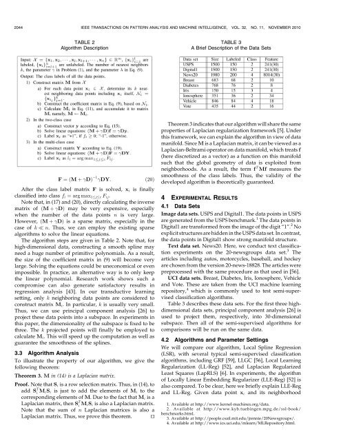
TABLE 3<br />
A Brief Description of the Data Sets<br />
F ¼ðM þ DÞ 1 DY:<br />
ð20Þ<br />
After the class label matrix F is solved, x i is finally<br />
classified into class f i ¼ arg max 1jc F ij .<br />
Note that, in (17) and (20), directly calculating the inverse<br />
matrix of ðM þ DÞ may be very expensive, especially<br />
when the number of the data points n is very large.<br />
However, ðM þ DÞ is a sparse matrix, especially in the<br />
case of k n. Thus, we can employ the existing sparse<br />
algorithms to solve the linear equations.<br />
The algorithm steps are given in Table 2. Note that, for<br />
high-dimensional data, constructing a smooth spline may<br />
need a huge number of primitive polynomials. As a result,<br />
the size of the coefficient matrix in (9) will become very<br />
large. Solving the equations could be uneconomical or even<br />
impossible. In practice, an alternative way is to only keep<br />
the linear polynomial. Research work shows such a<br />
compromise can also generate satisfactory results in<br />
regression analysis [43]. In our transductive learning<br />
setting, only k neighboring data points are considered to<br />
construct matrix M i . In particular, k is usually very small.<br />
Thus, we can use principal component analysis [26] to<br />
project these data points into a subspace. In experiments in<br />
this paper, the dimensionality of the subspace is fixed to be<br />
three. The k projected points will finally be employed to<br />
calculate M i . This will speed up the computation as well as<br />
guarantee the smoothness of the splines.<br />
3.3 Algorithm Analysis<br />
To illustrate the property of our algorithm, we give the<br />
following theorem:<br />
Theorem 3. M in (14) is a Laplacian matrix.<br />
Proof. Note that S i is a row selection matrix. Thus, in (14), to<br />
add S T i M iS i is just to add the elements of M i to the<br />
corresponding elements of M. Due to the fact that M i is a<br />
Laplacian matrix, then S T i M iS i is also a Laplacian matrix.<br />
Note that the sum of n Laplacian matrices is also a<br />
Laplacian matrix. Thus, we prove this theorem. tu<br />
Theorem 3 indicates that our algorithm will share the same<br />
properties of Laplacian regularization framework [5]. Under<br />
this framework, we can explain the algorithm in view of data<br />
manifold. Since M is a Laplacian matrix, it can be viewed as a<br />
Laplacian-Beltrami operator on data manifold, which treats f<br />
(here discretized as a vector) as a function on this manifold<br />
such that the global geometry of data is exploited from<br />
neighborhoods. As a result, the term f T Mf measures the<br />
smoothness of the class labels. Thus, the validity of the<br />
developed algorithm is theoretically guaranteed.<br />
4 EXPERIMENTAL RESULTS<br />
4.1 Data Sets<br />
Image data sets. USPS and Digital1. The data points in USPS<br />
are generated from the USPS benchmark. 1 The data points in<br />
Digital1 are transformed from the image of the digit “1”. 2 No<br />
explicit structures are hidden in the USPS data set. In contrast,<br />
the data points in Digital1 show strong manifold structure.<br />
Text data set. News20. Here, we conduct text classification<br />
experiments on the 20-newsgroups data set. 3 The<br />
articles including autos, motorcycles, baseball, and hockey<br />
are chosen from the version 20-news-18828. The articles were<br />
preprocessed with the same procedure as that used in [56].<br />
UCI data sets. Breast, Diabetes, Iris, Ionosphere, Vehicle<br />
and Vote. These are taken from the UCI machine learning<br />
repository, 4 which is commonly used to test semi-supervised<br />
classification algorithms.<br />
Table 3 describes these data sets. For the first three highdimensional<br />
data sets, principal component analysis [26] is<br />
used to project them, respectively, into 30-dimensional<br />
subspace. Then all of the semi-supervised algorithms for<br />
comparisons will be run on the same data.<br />
4.2 Algorithms and Parameter Settings<br />
We will compare our algorithm, <strong>Local</strong> <strong>Spline</strong> <strong>Regression</strong><br />
(LSR), with several typical semi-supervised classification<br />
algorithms, including GRF [59], LLGC [56], <strong>Local</strong> Learning<br />
Regularization (LL-Reg) [52], and Laplacian Regularized<br />
Least Squares (LapRLS) [6]. In experiments, the algorithm<br />
of <strong>Local</strong>ly Linear Embedding Regularizer (LLE-Reg) [52] is<br />
also compared. To be clear, here we briefly explain LLE-Reg<br />
and LL-Reg. Given data point x i and its neighborhood<br />
1. Available at http://www.kernel-machines.org/data.<br />
2. Available at http://www.kyb.tuebingen.mpg.de/ssl-book/<br />
benchmarks.html.<br />
3. Available at http://people.csail.mit.edu/jrennie/20Newsgroups/.<br />
4. Available at http://www.ics.uci.edu/mlearn/MLRepository.html.