Estimation of the extreme value index and high quantiles under ...
Estimation of the extreme value index and high quantiles under ...
Estimation of the extreme value index and high quantiles under ...
Create successful ePaper yourself
Turn your PDF publications into a flip-book with our unique Google optimized e-Paper software.
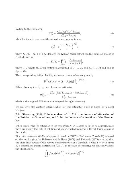
leading to <strong>the</strong> estimator<br />
H (c)<br />
Z,t =<br />
∑ ni=1<br />
log(Z i /t)1l {Zi >t}<br />
∑ ni=1<br />
, (6)<br />
δ i 1l {Zi >t}<br />
while for <strong>the</strong> <strong>extreme</strong> quantile estimator we propose to use<br />
ˆx (c)<br />
p,t = t<br />
( 1 − ˆFn (t)<br />
p<br />
) H<br />
(c)<br />
Z,t<br />
, (7)<br />
where ˆF n (x), −∞ < x < τ H denotes <strong>the</strong> Kaplan-Meier (1958) product limit estimator <strong>of</strong><br />
F (x), defined as<br />
1 − ˆF<br />
n∏<br />
[<br />
n (x) = 1 − δ ]<br />
j,n1l Zj,n ≤x<br />
,<br />
n − j + 1<br />
j=1<br />
where Z j,n denote <strong>the</strong> order statistics associated to Z 1 , ..., Z n <strong>and</strong> δ j,n := δ k if <strong>and</strong> only if<br />
Z j,n = Z k .<br />
The corresponding tail probability estimator is now <strong>of</strong> course given by<br />
IP ˆ<br />
(c) (X > x) = (1 − ˆF n (t)) ( x) (c) −1/H Z,t<br />
. (8)<br />
t<br />
When choosing t = Z n−k,n , we obtain <strong>the</strong> estimator<br />
H (c)<br />
Z,k,n = ∑ kj=1<br />
(<br />
log(Zn−j+1,n ) − log(Z n−k,n ) )<br />
∑ kj=1<br />
δ n−j+1,n<br />
, (9)<br />
which is <strong>the</strong> original Hill estimator adapted for right censoring.<br />
We will give also ano<strong>the</strong>r interpretation for this estimator which is based on a novel<br />
QQ-plot.<br />
2.2. Observing (Z, δ), X independent <strong>of</strong> Y , X in <strong>the</strong> domain <strong>of</strong> attraction <strong>of</strong><br />
<strong>the</strong> Fréchet or Gumbel law, <strong>and</strong> Y in <strong>the</strong> domain <strong>of</strong> attraction <strong>of</strong> <strong>the</strong> Fréchet<br />
law<br />
When considering <strong>the</strong> extension to <strong>the</strong> case where γ 1 ≥ 0, again as in <strong>the</strong> no-censoring case<br />
<strong>the</strong>re are mainly two sets <strong>of</strong> solutions which originated from two different formulations <strong>of</strong><br />
<strong>the</strong> model.<br />
First, <strong>the</strong> maximum likelihood approach based on POT’s (Peaks over Threshold) is based<br />
on <strong>the</strong> results given by Balkema <strong>and</strong> de Haan (1974) <strong>and</strong> Pick<strong>and</strong>s (1975), stating that<br />
<strong>the</strong> limit distribution <strong>of</strong> <strong>the</strong> absolute exceedances over a threshold t when t → ∞ is given<br />
by a generalized Pareto distribution (GPD). In <strong>the</strong> case <strong>of</strong> censoring, we can easily adapt<br />
<strong>the</strong> likelihood to<br />
k∏ [<br />
fGP D (Ẽj) ] δ j<br />
[<br />
1 − FGP D (Ẽj) ] 1−δ j<br />
j=1<br />
4


