Estimation of the extreme value index and high quantiles under ...
Estimation of the extreme value index and high quantiles under ...
Estimation of the extreme value index and high quantiles under ...

Create successful ePaper yourself
Turn your PDF publications into a flip-book with our unique Google optimized e-Paper software.
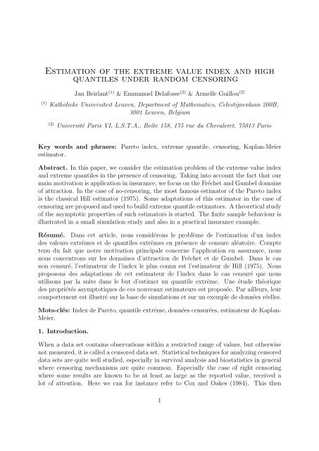
<strong>Estimation</strong> <strong>of</strong> <strong>the</strong> <strong>extreme</strong> <strong>value</strong> <strong>index</strong> <strong>and</strong> <strong>high</strong><br />
<strong>quantiles</strong> <strong>under</strong> r<strong>and</strong>om censoring<br />
Jan Beirlant (1) & Emmanuel Delafosse (2) & Armelle Guillou (2)<br />
(1) Katholieke Universiteit Leuven, Department <strong>of</strong> Ma<strong>the</strong>matics, Celestijnenlaan 200B,<br />
3001 Leuven, Belgium<br />
(2) Université Paris VI, L.S.T.A., Boîte 158, 175 rue du Chevaleret, 75013 Paris<br />
Key words <strong>and</strong> phrases: Pareto <strong>index</strong>, <strong>extreme</strong> quantile, censoring, Kaplan-Meier<br />
estimator.<br />
Abstract. In this paper, we consider <strong>the</strong> estimation problem <strong>of</strong> <strong>the</strong> <strong>extreme</strong> <strong>value</strong> <strong>index</strong><br />
<strong>and</strong> <strong>extreme</strong> <strong>quantiles</strong> in <strong>the</strong> presence <strong>of</strong> censoring. Taking into account <strong>the</strong> fact that our<br />
main motivation is application in insurance, we focus on <strong>the</strong> Fréchet <strong>and</strong> Gumbel domains<br />
<strong>of</strong> attraction. In <strong>the</strong> case <strong>of</strong> no-censoring, <strong>the</strong> most famous estimator <strong>of</strong> <strong>the</strong> Pareto <strong>index</strong><br />
is <strong>the</strong> classical Hill estimator (1975). Some adaptations <strong>of</strong> this estimator in <strong>the</strong> case <strong>of</strong><br />
censoring are proposed <strong>and</strong> used to build <strong>extreme</strong> quantile estimators. A <strong>the</strong>oretical study<br />
<strong>of</strong> <strong>the</strong> asymptotic properties <strong>of</strong> such estimators is started. The finite sample behaviour is<br />
illustrated in a small simulation study <strong>and</strong> also in a practical insurance example.<br />
Résumé. Dans cet article, nous considérons le problème de l’estimation d’un <strong>index</strong><br />
des valeurs extrêmes et de <strong>quantiles</strong> extrêmes en présence de censure aléatoire. Compte<br />
tenu du fait que notre motivation principale concerne l’application en assurance, nous<br />
nous concentrons sur les domaines d’attraction de Fréchet et de Gumbel. Dans le cas<br />
non censuré, l’estimateur de l’<strong>index</strong> le plus connu est l’estimateur de Hill (1975). Nous<br />
proposons des adaptations de cet estimateur de l’<strong>index</strong> dans le cas censuré que nous<br />
utilisons par la suite dans le but d’estimer un quantile extrême. Une étude théorique<br />
des propriétés asymptotiques de ces nouveaux estimateurs est proposée. Par ailleurs, leur<br />
comportement est illustré sur la base de simulations et sur un exemple de données réelles.<br />
Mots-clés: Index de Pareto, quantile extrême, données censurées, estimateur de Kaplan-<br />
Meier.<br />
1. Introduction.<br />
When a data set contains observations within a restricted range <strong>of</strong> <strong>value</strong>s, but o<strong>the</strong>rwise<br />
not measured, it is called a censored data set. Statistical techniques for analyzing censored<br />
data sets are quite well studied, especially in survival analysis <strong>and</strong> biostatistics in general<br />
where censoring mechanisms are quite common. Especially <strong>the</strong> case <strong>of</strong> right censoring<br />
where some results are known to be at least as large as <strong>the</strong> reported <strong>value</strong>, received a<br />
lot <strong>of</strong> attention. Here we can for instance refer to Cox <strong>and</strong> Oakes (1984). This <strong>the</strong>n<br />
1
concerns central characteristics <strong>of</strong> <strong>the</strong> <strong>under</strong>lying distribution. The literature on tail or<br />
<strong>extreme</strong> <strong>value</strong> analysis for censored data is almost non existing. In Reiss <strong>and</strong> Thomas<br />
(1997) (section 6.1), Beirlant et al. (1996) (section 2.7) <strong>and</strong> Beirlant <strong>and</strong> Guillou (2001) in<br />
case <strong>of</strong> truncated data, some estimators <strong>of</strong> tail indices were proposed without any deeper<br />
study on <strong>the</strong>ir behaviour. However, important problems such as <strong>the</strong> estimation <strong>of</strong> <strong>extreme</strong><br />
<strong>quantiles</strong> apparently were not considered before in general.<br />
Data sets with censored <strong>extreme</strong> data <strong>of</strong>ten occur in insurance when reported payments<br />
cannot be larger than <strong>the</strong> maximum payment <strong>value</strong> <strong>of</strong> <strong>the</strong> contract. When <strong>the</strong> reported<br />
payment equals <strong>the</strong> maximum payment, this real payment can indeed be equal to <strong>the</strong><br />
maximum or can be censored. The situation where all data above a fixed <strong>value</strong> are<br />
censored is referred to as truncation or type I censoring. This case was considered in<br />
Beirlant <strong>and</strong> Guillou (2001). It can occur when <strong>the</strong> observations are not <strong>the</strong> real payments<br />
but <strong>the</strong> payments as a fraction <strong>of</strong> <strong>the</strong> sum insured, in which case <strong>the</strong> truncation level equals<br />
100%. Here we consider r<strong>and</strong>om right censoring. The claim sizes X are possibly censored<br />
by <strong>the</strong> maximum payment Y . A maximum payment <strong>of</strong> a given contract is <strong>the</strong>n considered<br />
as a realization <strong>of</strong> <strong>the</strong> r<strong>and</strong>om variable Y . Different situations can now occur, whe<strong>the</strong>r<br />
<strong>the</strong> censoring <strong>value</strong>s (or maximum payment <strong>value</strong>s) are observed or not.<br />
To be more specific, let X i , i ∈ IN, be independent <strong>and</strong> identically distributed (i.i.d.)<br />
r<strong>and</strong>om variables with common distribution function (df) F <strong>and</strong> let Y i , i ∈ IN, be a<br />
second i.i.d. sequence with df G. We only observe Z i = X i ∧ Y i , δ i = 1l Xi ≤Y i<br />
, i ∈ IN. We<br />
denote by H <strong>the</strong> df <strong>of</strong> Z 1 <strong>and</strong> let τ H = inf{x : H(x) = 1}, <strong>the</strong> supremum <strong>of</strong> <strong>the</strong> support<br />
<strong>of</strong> H. We define H 1 (z) = IP(Z > z, δ = 1) = IP(z < X ≤ Y ).<br />
Being motivated by actuarial applications we confine ourselves to <strong>the</strong> case where sample<br />
maxima from X samples are in <strong>the</strong> domain <strong>of</strong> attraction <strong>of</strong> <strong>the</strong> Fréchet or Gumbel law.<br />
This typically means that we consider polynomially decreasing tails or exponentially decreasing<br />
tails with infinite right endpoint. We will consequently consider <strong>the</strong> following<br />
cases:<br />
• Observing (Z, δ), X independent <strong>of</strong> Y , <strong>and</strong> both X <strong>and</strong> Y are in <strong>the</strong> domain <strong>of</strong> attraction<br />
<strong>of</strong> <strong>the</strong> Fréchet law;<br />
• Observing (Z, δ), X independent <strong>of</strong> Y , X is in <strong>the</strong> domain <strong>of</strong> attraction <strong>of</strong> <strong>the</strong> Fréchet<br />
or <strong>the</strong> Gumbel law, <strong>and</strong> Y in <strong>the</strong> domain <strong>of</strong> attraction <strong>of</strong> <strong>the</strong> Fréchet law.<br />
In order to illustrate <strong>the</strong> methods presented in this paper, we use a liability insurance<br />
example from Frees <strong>and</strong> Valdez (1998).<br />
2. <strong>Estimation</strong> techniques.<br />
2.1. Observing (Z, δ), X independent <strong>of</strong> Y , <strong>and</strong> both X <strong>and</strong> Y are in <strong>the</strong> domain<br />
<strong>of</strong> attraction <strong>of</strong> <strong>the</strong> Fréchet law<br />
2
Supposing that F is <strong>of</strong> Pareto-type, that is, <strong>the</strong>re exists a positive constant α for which<br />
where l 1 is a slowly varying function at infinity satisfying<br />
1 − F (x) = x −α l 1 (x), (1)<br />
l 1 (λx)<br />
l 1 (x)<br />
→ 1 when x → ∞, for all λ > 0.<br />
In order for <strong>the</strong> censoring to be not too heavy, it appears natural to assume that <strong>the</strong><br />
censoring distribution is also heavy tailed<br />
1 − G(x) = x −β l 2 (x), (2)<br />
for some β > 0 <strong>and</strong> slowly varying l 2 . Assuming that X <strong>and</strong> Y are independent, so that<br />
1 − H(x) = (1 − F (x))(1 − G(x)), it now follows that<br />
1 − H(x) = x −(α+β)˜l(x), (3)<br />
with ˜l also a slowly varying function at infinity. These conditions can be restated in terms<br />
<strong>of</strong> <strong>the</strong> tail quantile functions as<br />
U F (x) = x 1/α l 1,U (x), U G (x) = x 1/β l 2,U (x), U H (x) = x 1/(α+β)˜lU (x),<br />
with U F (x) = inf{y : F (y) ≥ 1 − 1/x}, x > 1, <strong>and</strong> l 1,U (x), l 2,U (x) <strong>and</strong> ˜l U (x) again slowly<br />
varying functions at infinity.<br />
Our goal is( to ) discuss <strong>the</strong> estimation problem <strong>of</strong> γ 1 := α −1 <strong>and</strong> <strong>of</strong> <strong>extreme</strong>s <strong>quantiles</strong><br />
x F,p := U 1<br />
F p with p <<br />
1<br />
. This problem has received a lot <strong>of</strong> attention in case <strong>of</strong> nocensoring,<br />
i.e. when X i ≤ Y i for all i = 1, ..., n. The most famous estimator <strong>of</strong> γ 1 is Hill’s<br />
n<br />
(1975) estimator, given by<br />
H X,k,n = 1 k∑<br />
log X n−i+1,n − log X n−k,n . (4)<br />
k<br />
i=1<br />
Turning to <strong>the</strong> estimation <strong>of</strong> <strong>high</strong> <strong>quantiles</strong>, <strong>the</strong> estimator proposed by Weissman (1978)<br />
serves as a reference <strong>under</strong> Pareto-type models without censoring:<br />
ˆx p,k = X ( k + 1 ) HX,k,n<br />
n−k,n . (5)<br />
(n + 1)p<br />
In case <strong>of</strong> r<strong>and</strong>om right censoring, <strong>the</strong> likelihood based on E j,t = Z j<br />
, Z t j > t, is changed<br />
into<br />
∏N t ( )<br />
αE<br />
−α−1 δj<br />
( )<br />
j E<br />
−α 1−δj<br />
j ,<br />
j=1<br />
3
leading to <strong>the</strong> estimator<br />
H (c)<br />
Z,t =<br />
∑ ni=1<br />
log(Z i /t)1l {Zi >t}<br />
∑ ni=1<br />
, (6)<br />
δ i 1l {Zi >t}<br />
while for <strong>the</strong> <strong>extreme</strong> quantile estimator we propose to use<br />
ˆx (c)<br />
p,t = t<br />
( 1 − ˆFn (t)<br />
p<br />
) H<br />
(c)<br />
Z,t<br />
, (7)<br />
where ˆF n (x), −∞ < x < τ H denotes <strong>the</strong> Kaplan-Meier (1958) product limit estimator <strong>of</strong><br />
F (x), defined as<br />
1 − ˆF<br />
n∏<br />
[<br />
n (x) = 1 − δ ]<br />
j,n1l Zj,n ≤x<br />
,<br />
n − j + 1<br />
j=1<br />
where Z j,n denote <strong>the</strong> order statistics associated to Z 1 , ..., Z n <strong>and</strong> δ j,n := δ k if <strong>and</strong> only if<br />
Z j,n = Z k .<br />
The corresponding tail probability estimator is now <strong>of</strong> course given by<br />
IP ˆ<br />
(c) (X > x) = (1 − ˆF n (t)) ( x) (c) −1/H Z,t<br />
. (8)<br />
t<br />
When choosing t = Z n−k,n , we obtain <strong>the</strong> estimator<br />
H (c)<br />
Z,k,n = ∑ kj=1<br />
(<br />
log(Zn−j+1,n ) − log(Z n−k,n ) )<br />
∑ kj=1<br />
δ n−j+1,n<br />
, (9)<br />
which is <strong>the</strong> original Hill estimator adapted for right censoring.<br />
We will give also ano<strong>the</strong>r interpretation for this estimator which is based on a novel<br />
QQ-plot.<br />
2.2. Observing (Z, δ), X independent <strong>of</strong> Y , X in <strong>the</strong> domain <strong>of</strong> attraction <strong>of</strong><br />
<strong>the</strong> Fréchet or Gumbel law, <strong>and</strong> Y in <strong>the</strong> domain <strong>of</strong> attraction <strong>of</strong> <strong>the</strong> Fréchet<br />
law<br />
When considering <strong>the</strong> extension to <strong>the</strong> case where γ 1 ≥ 0, again as in <strong>the</strong> no-censoring case<br />
<strong>the</strong>re are mainly two sets <strong>of</strong> solutions which originated from two different formulations <strong>of</strong><br />
<strong>the</strong> model.<br />
First, <strong>the</strong> maximum likelihood approach based on POT’s (Peaks over Threshold) is based<br />
on <strong>the</strong> results given by Balkema <strong>and</strong> de Haan (1974) <strong>and</strong> Pick<strong>and</strong>s (1975), stating that<br />
<strong>the</strong> limit distribution <strong>of</strong> <strong>the</strong> absolute exceedances over a threshold t when t → ∞ is given<br />
by a generalized Pareto distribution (GPD). In <strong>the</strong> case <strong>of</strong> censoring, we can easily adapt<br />
<strong>the</strong> likelihood to<br />
k∏ [<br />
fGP D (Ẽj) ] δ j<br />
[<br />
1 − FGP D (Ẽj) ] 1−δ j<br />
j=1<br />
4
where Ẽj = Z j − t if Z j > t <strong>and</strong> 1 − F GP D (x) = ( )<br />
1 + γ −<br />
1<br />
1x γ 1<br />
. Then, <strong>the</strong> maximization <strong>of</strong><br />
σ<br />
this expression leads to a POT estimator for γ 1 which we fur<strong>the</strong>r denote by ˆγ t,ML.<br />
(c)<br />
Secondly, we can construct a new estimator based on k upper order statistics for instance<br />
within <strong>the</strong> framework <strong>of</strong> <strong>the</strong> QQ-plot regression technique. For example, in <strong>the</strong> case <strong>of</strong><br />
no-censoring, Beirlant et al. (1996) proposed an estimator <strong>of</strong> a real-<strong>value</strong>d <strong>index</strong> based on<br />
a generalized quantile plot, which takes over <strong>the</strong> role <strong>of</strong> <strong>the</strong> Pareto quantile plot in this<br />
more general setting. More precisely <strong>the</strong>y proposed to look at <strong>the</strong> graph with coordinates<br />
( n + 1<br />
)<br />
log , log UH j,n , j = 1, ..., n − 1,<br />
j<br />
with UH j,n = X n−j,n H X,j,n . Again this plot becomes ultimately linear for small j with<br />
slope approximating γ 1 . Then, one can construct several regression based estimators, such<br />
as<br />
ˆγ k,UH = 1 k∑<br />
log UH j,n − log UH k+1,n .<br />
k<br />
j=1<br />
From <strong>the</strong> above it appears natural to define a generalization <strong>of</strong> ˆγ k,UH to <strong>the</strong> censoring<br />
case as a slope estimator <strong>of</strong> <strong>the</strong> generalized quantile plot adapted for censoring<br />
( (<br />
− log 1 − ˆFn (Z n−j+1,n ) ) , log UH j,n) (c) , (10)<br />
(j = 1, ..., n − 1) where UH (c)<br />
j,n = Z n−j,n H (c)<br />
Z,j,n:<br />
ˆγ (c)<br />
1 ∑ kj=1<br />
k,UH = log UH (c)<br />
k<br />
1<br />
k<br />
j,n − log UH (c)<br />
k+1,n<br />
∑ kj=1<br />
. (11)<br />
δ n−j+1,n<br />
Using one <strong>of</strong> <strong>the</strong> abovementioned estimators ˆγ (c)<br />
.,. <strong>of</strong> γ 1 ≥ 0 we can now propose new<br />
estimators for <strong>the</strong> quantile x F,p , in <strong>the</strong> spirit <strong>of</strong> <strong>the</strong> one proposed by Dekkers et al. (1989)<br />
in <strong>the</strong> case <strong>of</strong> no-censoring:<br />
ˆx (c)<br />
p,t,. = t + ˆγ (c)<br />
.,. t<br />
( 1− ˆFn(t)<br />
)ˆγ (c)<br />
.,.<br />
p<br />
ˆγ (c)<br />
.,.<br />
− 1<br />
. (12)<br />
Under suitable assumptions, we establish <strong>the</strong> asymptotic properties <strong>of</strong> our estimators. We<br />
illustrate <strong>the</strong>ir behaviour in a small simulation study, but also in a practical insurance<br />
example.<br />
5
Bibliography<br />
[1] Balkema, A. <strong>and</strong> de Haan, L. (1974). Residual life time at great age, Ann. Probab.,<br />
2, 792-804.<br />
[2] Beirlant, J. <strong>and</strong> Guillou, A. (2001). Pareto <strong>index</strong> estimation <strong>under</strong> moderate right<br />
censoring, Sc<strong>and</strong>. Actuarial J., 2, 111-125.<br />
[3] Beirlant, J. Teugels, J.L. <strong>and</strong> Vynckier, P. (1996). Practical Analysis <strong>of</strong> Extreme<br />
Values, Leuven University Press, Leuven.<br />
[4] Beirlant, J., Vynckier, P. <strong>and</strong> Teugels, J.L. (1996). Excess functions <strong>and</strong> estimation <strong>of</strong><br />
<strong>the</strong> <strong>extreme</strong> <strong>value</strong> <strong>index</strong>, Bernoulli, 2, 293-318.<br />
[5]Cox, D.R. <strong>and</strong> Oakes, D (1984). Analysis <strong>of</strong> Survival Data, Chapman <strong>and</strong> Hall, New<br />
York.<br />
[6] Dekkers, A.L.M., Einmahl, J.H.J. <strong>and</strong> de Haan, L. (1989). A moment estimator for<br />
<strong>the</strong> <strong>index</strong> <strong>of</strong> an <strong>extreme</strong>-<strong>value</strong> distribution, Ann. Statist. 17, 1833-1855.<br />
[7] Frees, E. <strong>and</strong> Valdez, E. (1998). Underst<strong>and</strong>ing relationships using copulas, North<br />
American Actuarial Journal, 2, 1–15.<br />
[8] Hill, B.M. (1975). A simple general approach to inference about <strong>the</strong> tail <strong>of</strong> a distribution,<br />
Ann. Statist., 3, 1163-1174.<br />
[9] Kaplan, E.L. <strong>and</strong> Meier, P. (1958). Non-parametric estimation from incomplete observations,<br />
J. Amer. Statist. Assoc., 53, 457-481.<br />
[10] Pick<strong>and</strong>s III, J. (1975). Statistical inference using <strong>extreme</strong> order statistics, Ann.<br />
Statist., 3, 119-131.<br />
[11] Reiss, R.D. <strong>and</strong> Thomas, M. (1997). Statistical Analysis <strong>of</strong> Extreme Values with<br />
Applications to Insurance, Finance, Hydrology <strong>and</strong> O<strong>the</strong>r Fields, Birkhäuser Verlag, Basel.<br />
[12] Weissman, I. (1978). <strong>Estimation</strong> <strong>of</strong> parameters <strong>and</strong> large <strong>quantiles</strong> based on <strong>the</strong> k<br />
largest observations. J. Amer. Statist. Assoc. 73, 812-815.<br />
6