Download Paper - Computer Graphics - University of California ...

New 3D Graphics Rendering Engine Architecture for 

Direct Tessellation of Spline Surfaces 

Dr. Adrian Sfarti, Prof. Brian Barsky, Todd Kosloff, Egon Pasztor, Alex Kozlowski, Eric Roman 

Alex Perelman, Ali El-Annan, Tim Wong, Grace Chen, Clarence Tam and Chris Lai 

Abstract 

In current 3D graphics architectures, the bus between the triangle server and the rendering engine GPU is clogged 

with triangle vertices and their many attributes (normal vectors, colors, texture coordinates). We develop a new 

3D graphics architecture using data compression to unclog the bus between the triangle server and the rendering 

engine. The data compression is achieved by replacing the conventional idea of a GPU that renders triangles with 

a GPU that tessellates surface patches into triangles. 

Categories and Subject Descriptors (according to ACM 

CCS): B.4.2 [Computer Graphics]: Hardware Architecture/Graphics 

Processors; I.3.3 [Computer Graphics]: Picture/Image 

Generation/Curve Generation 

1. Introduction 

AGP 

CPU 

3D Application 

3D API 

Programmable 

Vertex Processor 

Primitive 

Assembly 

Rasterization & 

Interpolation 

Programmable 

Pixel Processor 

Raster 

Operations 

Framebuffer 

GPU 

Triangle Vertices 

AGP 

CPU 

3D Application 

3D API 

Programmable 

Control Point 

Processor 

Tessellation 

Programmable 

Vertex Processor 

Primitive 

Assembly 

Rasterization & 

Interpolation 

Programmable 

Pixel Processor 

Raster 

Operations 

Framebuffer 

GPU 

Surface Control points 

Triangle Vertices 

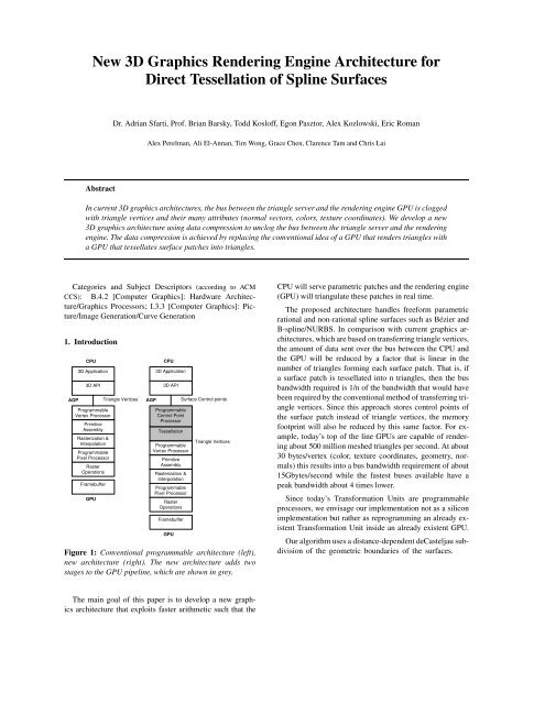
Figure 1: Conventional programmable architecture (left), 

new architecture (right). The new architecture adds two 

stages to the GPU pipeline, which are shown in grey. 

CPU will serve parametric patches and the rendering engine 

(GPU) will triangulate these patches in real time. 

The proposed architecture handles freeform parametric 

rational and non-rational spline surfaces such as Bézier and 

B-spline/NURBS. In comparison with current graphics architectures, 

which are based on transferring triangle vertices, 

the amount of data sent over the bus between the CPU and 

the GPU will be reduced by a factor that is linear in the 

number of triangles forming each surface patch. That is, if 

a surface patch is tessellated into n triangles, then the bus 

bandwidth required is 1/n of the bandwidth that would have 

been required by the conventional method of transferring triangle 

vertices. Since this approach stores control points of 

the surface patch instead of triangle vertices, the memory 

footprint will also be reduced by this same factor. For example, 

today’s top of the line GPUs are capable of rendering 

about 500 million meshed triangles per second. At about 

30 bytes/vertex (color, texture coordinates, geometry, normals) 

this results into a bus bandwidth requirement of about 

15Gbytes/second while the fastest buses available have a 

peak bandwidth about 4 times lower. 

Since today’s Transformation Units are programmable 

processors, we envisage our implementation not as a silicon 

implementation but rather as reprogramming an already existent 

Transformation Unit inside an already existent GPU. 

Our algorithm uses a distance-dependent deCasteljau subdivision 

of the geometric boundaries of the surfaces. 

The main goal of this paper is to develop a new graphics 

architecture that exploits faster arithmetic such that the

2 Dr. Adrian Sfarti, Prof. Brian Barsky, Todd Kosloff, Egon Pasztor, Alex Kozlowski, Eric RomanAlex Perelman, Ali El-Annan, Tim Wong, Grace Chen, Clarence Tam and Chr 

o 

2. Previous Work 

There have been very few implementations of real time tesselation 

in hardware. In the mid-1980’s, Sun developed an 

architecture for this that was described in [LSP87] and in 

a series of associated patents. The implementation was not 

a significant technical or commercial success because it did 

not exploit triangle based rendering; instead it attempted to 

render the surfaces in a pixel-by-pixel manner [LS87]. The 

idea was to use adaptive forward differencing to interpolate 

infinitesimally close parallel cubic curves imbedded into the 

bicubic surface. 

More recently, Henry Moreton from NVIDIA has resurrected 

the real time tesselation unit [Mor03]. This method 

does not directly tesselate patches in real time; rather, it uses 

off-line pre-tesselated triangle meshes in conjunction with a 

proprietary stitching method that avoids cracking and popping 

at the seams. Using this approach, the tessellation unit 

exists in front of the transformation unit and outputs triangle 

databases to be rendered by the existent components of the 

3D graphics hardware. 

The current paper is based on a recent patent [Sfa03] that 

is the first to introduce a real time tesselation processor into 

a GPU pipeline. To date, there is no GPU built with a real 

time tesselator processor but we hope that the current article 

will spark the design of such a device. 

3. GPU Architectures 

3.1. Current State of the Art 

The pseudo code describing the current state of the art GPU 

architectures is shown below for the bicubic case. Notation: 

Let (s i ,t j ) denote a pair of parameter values used in patch parameterization, 

V i, j a vertex, and N i, j a vertex normal. Also, 

we denote texture coordinates by u i, j and v i, j . 

Step 1 (off-line) For each bicubic surface, subdivide the S 

and T intervals until each resultant four-sided surface is 

below a certain predetermined curvature value. 

Step 2 For all bicubic surfaces sharing a common boundary, 

take the union of the subdivisions to prevent cracks along 

the common boundary. 

Step 3 For each bicubic surface, For each pair (s i ,t j ), Calculate 

(u i, j ,v i, j ,q i, j ,V i, j ), Generate triangles by connecting 

neighboring vertices. 

Step 4 For each vertex V i, j Calculate the normal N i, j to that 

vertex (used for lighting). For each triangle Calculate the 

normal to the triangle (used for culling). 

Step 5 (real time) Transform the vertices V i, j and the normals 

N i, j and the normals to the triangles. For each vertex 

V i, j , Calculate lighting. 

3.2. The Tesselator Unit – Principles of Operation 

Though we have not implemented our proposed GPU in silicon 

yet we are publishing below the behavioral code 

describing the principles of operation. 

o 

Step 0 (all steps in real time) ( For each surface transform 

only 16 points instead of transforming all the vertices inside 

the surface. There is no need to transform the normals 

to the vertices since they are generated at step 4). For each 

bicubic surface Transform the 16 control points and the 

single normal that determine the surface. 

Step 1 (Simplify the three dimensional surface subdivision 

by reducing it to the subdivision of the cubic curves determined 

by the surface bounding box). For each bicubic 

surface, Subdivide the boundary curve representing the s 

interval until the projection of the length of the height of 

the curve bounding box is below a certain predetermined 

number of pixels as measured in screen coordinates. Subdivide 

the boundary curve representing the t interval until 

the projection of the length of the height of the curve 

bounding box is below a certain predetermined number of 

pixels as measured in screen coordinates. 

(Simplify the subdivision termination criterion by expressing 

it in screen (SC) coordinates and by measuring 

the curvature in pixels. For each new view, a new subdivision 

can be generated, producing automatic level of 

detail). 

Step 2 For all bicubic surfaces sharing a same parameter 

(either s or t) boundary, Choose as the common subdivision 

the reunion of the subdivisions in order to prevent 

cracks showing along the common boundary OR choose 

as the common subdivision the finest subdivision (the one 

with the most points inside the set) OR insert a zippering 

strip to smoothly progress from one patch to its neighbor. 

(Prevent cracks at the boundary between surfaces). 

Step 3 (Generate the vertices, normals, the texture coordinates 

and the displacements used for bump and displacement 

mapping for the present subdivision) For each bicubic 

surface, For each pair (s i ,t j ) (All calculations employ 

some form of direct evaluation of the variables) Calculate 

((u i, j ,v i, j ,q i, j ),(p i, j ,r i, j ),V i, j ) thru evaluation (texture 

, displacement map and vertex coordinates as a function 

of (s i ,t j )) Look up vertex displacement (dx i, j ,dy i, j ,dz i, j ). 

Generate triangles by connecting neighboring vertices. 

Step 4 For each vertex V i, j Calculate the normal N i, j to that 

vertex (Already transformed in WC) 

4. The Subdivision Step 

We use the Lane-Carpenter subdivision algorithm described 

in [LCWB80] but we apply our own termination criterion. 

The geometric adaptive subdivision induces a corresponding 

parametric subdivision. 

The following discussion assumes that the Bézier surface 

patch is bicubic, but that approach is valid for arbitrary degree. 

The four boundary curves of a Bézier patch are themselves 

Bézier curves, which we subdivide using the following 

formulas. We use the following notation: Let P 1 , P 2 , P 3 , 

and P 4 denote the four control points of such a curve. We 

denote the four control points of the left sub-curve by L 1 

through L 4 and the control points of the right sub-curve by 

R 1 through R 4 . Let H denote the midpoint of the line segment 

connecting P 2 to P 3 .

Dr. Adrian Sfarti, Prof. Brian Barsky, Todd Kosloff, Egon Pasztor, Alex Kozlowski, Eric RomanAlex Perelman, Ali El-Annan, Tim Wong, Grace Chen, Clarence Tam and Chris 

L 3 

H 

R 2 

S = [s 3 ,s 2 ,s,1] 

T = [t 3 ,t 2 ,t,1] T 

y(s,t) = S × M b × P y × M b × T 

z(s,t) = S × M b × P z × M b × T 

L 4 

= R 1 

R 3 

L 2 

P 1 

P 2 P 3 

P 4 

Figure 2: Curve Subdivision 

For constant S, the matrix M = S × M b × P z × 

M b is constant and the calculation of the vertices 

V (x(s,t),y(s,t),z(s,t)) reduces to the evaluation of the vector 

T plus the computing of the product M × T . Therefore, 

the generation of vertices is comparable with vertex transformation. 

Note that the vertices are generated already transformed 

in place because the parent bicubic surface has already 

been transformed. 

To determine the vertex normals for each generated vertex 

V i, j , we calculate the gradient to the surface. 

We calculate the texture coordinates through bilinear interpolation. 

The parametrization of the surface produces a 

natural interpolation of the texture coordinates (see Figure 3 

for details). 

L 1 = P 1 

L 2 = P 1 + P 2 

2 

H = P 2 + P 3 

2 

L 3 = L 2 + H 

2 

R 4 = P 4 

R 3 = P 3 + P 4 

2 

R 2 = R 3 + H 

2 

R 1 = L 4 = L 3 + R 2 

2 

The edge subdivision results in a subdivision of 

the parametric intervals s{s 0 ,s 1 ,...s i ,...s m } and 

t{t 0 ,t 1 ,...t j ,...t n }. These parameter values are stored, 

whereas the control points resulting from subdivision are 

discarded immediately after the termination test is run. 

After the subdivision and crack prevention steps, the actual 

vertex locations throughout the patch are computed from the 

stored parameter values, using the following formulas: Let 

x(s,t), y(s,t), and z(s,t) denote the functions that compute 

vertex locations from parameter values. Let S and T denote 

vectors containing the paramater values raised to powers 

one through three. We denote the Bernstein basis (expressed 

in matrix form) by M b . The matrices P x , P y and P z contain x, 

y, and z coordinates (respectively) of the 16 control points. 

V i j = V (x(s i ,t j ),y(s i ,t j ),z(s i ,t j ))i = 1,m, j = 1,n 

x(s,t) = S × M b × P x × M b × T 

P 21 

S=0, T=0 

P 2 (t) 

P 1 (t) 

P 32 

P 41 

P 3 (t) 

S=1, T=0 P 4 (t) 

P 33 

P 34 

P 12 

S=0, T=1 

P 44 

S=1, T=1 

5. Termination Criteria 

(0,1) 

Figure 3: Texture Coordinates 

V 

Texture Space 

(0,0) (1,0) 

Our algorithm decides that an edge curve has been sufficiently 

subdivided when the trapezoidal convex hull of that 

curve has a sufficiently small height, as seen from the viewpoint 

of the observer. Referring to Figure 4, subdivision terminates 

when the following condition is met: 

Maximum{distance(P 12 to line(P 11 ,P 14 )), 

2d 

distance(P 13 to line(P 11 ,P 14 ))} × (|P 12z |+|P 13z |) < n 

AND 

Maximum {distance(P 24 to line(P 14 ,P 44 )), 

2d 


where n is an arbitrary number expressed in pixels or in a 

fraction of pixels and d is the distance from the viewer to the 

projection plane. 

We experimented with n starting at 1 and we observed that 

there were artifacts, especially along the silhouette. Forsey 

et al. [FK90] seem to settle on n = .5 and we tried that. We 

(1,1) 

U


also experimented with n > 1, for reasons of rapid prototyping 

and previewing. The above criterion is sufficient for 

surface patches that are not more curved inside their boundaries 

than they are along their boundaries. The criterion ensures 

that abutting patches share the same subdivision along 

the common boundary. Conversely, if the patches are more 

curved inside than they are along their boundaries, we add a 

criterion that has a slightly modified form: 

Y 

Z 

P 21 

P 2 (t) 

P 1 (t) 

P 32 

P 3 (t) 

P 4 (t) 

P 33 

P 34 

P 12 

P 41 P 42 

P 43 

P 44 


2d 

distance(P 32 to line(P 42 ,P 12 ))} × (|P 42z |+|P 12z | < n 

AND 


2d 


Since the curvature of free-form surfaces can switch between 

being boundary-limited and internally-limited, we 

will need to measure the flatness of both types of curves at 

the start of the tesselation associated with each instance of 

the surface by subdividing the four boundary curves as well 

as two orthogonal internal curves, specifically the curves that 

interverne in the second termination criterion shown above. 

We can further exploit the fact that adjacent patches share 

two boundary curves so that we need to subdivide only two 

of the four boundary curves for each patch. The only obvious 

exceptions are the patches at the boundary of a surface, since 

such patches have fewer than four neighbors. In the case of 

the boundary patches, our algorithm always subdivides all 

four boundary curves. As long as abutting patches share the 

same boundary curves, this approach guarantees edge continuity 

between surfaces without the need to share any edge 

information between patches. 

Our termination test ensures that patches are subdivided 

sufficiently to avoid silhouette artifacts. However, the test 

was shown to be insufficient in the case of a large flat patch 

facing the viewer. Such a patch would not be subdivided because 

a single pair of triangles can completely capture the 

geometry of this curve. However, per-vertex lighting would 

lead to highlight artifacts. Additionally, nearly-flat portions 

of a patch exhibit undesirable texture flickering as they visibly 

transition from one level of detail to the next. This is 

because the bilinear texture coordinate interpolation that we 

use when assigning texture coordinates to triangle vertices is 

not the same as the method used to interpolate within a triangle. 

To combat this problem, we decree that patches must be 

subdivided a minimum number of times, regardless of curvature. 

6. Crack Prevention 

If there are no special prevention methods, cracks may 

appear at the boundary between abutting patches. This is 

mainly due to the fact that the patches are subdivided independently 

of each other. Abutting patches can exhibit different 

curvatures resulting in different subdivisions. For example, 

in Figure 7, we see that the right-hand patch has a 

finer subdivision than the left-hand one. At the boundary, we 

see how a “T-joint” has been formed. When rendering the 

parallel strips of triangles to the left and to the right of the 

d 

X 

Figure 4: Termination Criteria 

Figure 5: Without Crack Prevention (note cracks appearing 

around the handle in the middle of the lid of the teapot, and 

at the tip of the spout). 

common boundary, a crack may become visible in the area 

of the T-joint. 

If two patches bounding two separate surfaces share an 

edge curve, they share the same control points and they will 

share the same tesselation. By doing so we ensure the absence 

of cracks between patches that belong to data structures 

that have been dispatched independently and thus our 

method scales the exact same way the traditional triangle 

based method does. 

Zippering leaves the interior of patches untouched, allowing 

these regions to be tessellated without concern for 

neighboring patches. To eliminate cracks between adjacent 

patches (as in Figure 5), the portion of a patch that is immediately 

in contact with an adjacent patch is carefully tessellated 

using a zipper-like configuration, so as to seamlessly 

move from a lower to higher level of tesselation. An example 

of zippering is shown in Figure 8. 

We tested the crack prevention algorithm on a large selection 

of objects, making sure that the method works on corner 

cases such as the fans of patches shown in figure 8. 

7. Performance Measurements 

In order to measure the performance of the algorithm, we 

tested our prototype on five dynamic scenes. Each scene


Figure 6: With Crack Prevention 

Figure 8: Zippering In Action 

the main performance savings in our architecture will come 

from the AGP/PCIX bus bandwidth reduction we wanted to 

verify that our approach does not create a bottleneck inside 

the GPU. We obtained ample proof that this is not the case 

by trying many scenarios that allow for complex animations 

of flocks of objects in the context of a variable viewpoint . 

We have made several movies of our animations as well as a 

menu driven interactive demo. 

T-Join 

Figure 7: Cracking 

comprised seven teapots that were spun along different elliptical 

paths. At any given moment, some teapots are close 

to the viewer, while others are far away. We recorded the average 

time it took to tessellate each scene (in milliseconds) 

as well as the average frames rate. Our back-patch culling 

feature was turned on. 

All tests were performed on a Pentium 4 2.4Ghz machine 

with a GeForce4 MX440 video card. We realize that the performance 

testing is done on a software simulation of the Tesselator 

Unit architecture since none of the existent GPU’s 

has one today. Therefore, the performance numbers are only 

indicative of the performance of the actual architecture. Nevertheless, 

it was immediately observed that the dynamic tessellation 

compares favorably with the fixed tesselation since 

it shows higher frame rates in most cases, as described below. 

The quality of the rendering is improved as well , especially 

for the cases when the objects are very close to 

the viewer. We observed no disadvantages to our method 

as compared to the conventional method. We experimented 

with a scene that had a fixed tesselation of 64k triangles. By 

using the real time tesselation the number of triangles varied 

from a maximum of 16k (closest from the viewer) down 

to a few hundreds (farthest from the viewer) clearly demonstrating 

the compression capabilities of our method. Since 

Figure 9 shows an average of the values obtained during 

the testing of all five scenes, all results in expressed in 

“frames per second” (fps). 

The “RTT” entry represents our real time tesselation 

method. We separated the measurements into transform+tesselate 

only vs. transform+tesselate+render. The 

reason is that we wanted to measure the exact effects of the 

tesselation by comparison with conventional offline tesselation. 

In a real GPU there would be a tesselator unit stage, 

so that the effects of tesselation on execution time would be 

hidden by the fact that the GPU is pipelined. We rendered 

the same animation four different times, each time at a different 

criterion of subdivision termination (n = 0.5, n = 0.7, 

n = 1, n = 2). As n (the fractional deviation of the planar 

approximation from the real surface, expressed in pixels) increases, 

the number of triangles generated from subdivision 

decreases and the speed increases. 

We also implemented a feature to simulate the current 

standard rendering methods whereby models are tessellated 

offline and then sent to the GPU as sets of triangles. This 

is the “Offline Tesselation” entry at the bottom of the table. 

Each patch is tessellated uniformly to a user-defined number 

of triangles (128, 512, or 2048). On every frame, each 

pre-calculated vertex is transformed from model space into 

world coordinates. The normal of each vertex is also appropriately 

transformed into world coordinates. Then the triangle 

is rendered directly. 

In all scenes, because the number of triangles remains 

constant between frames and no dynamic tessellation occurs, 

there was negligible deviation between values obtained 

while rendering different scenes. Figure 9 shows the timings 

obtained on all scenes tested.


Triangles 

Generated 

RTT 

Transform + Tessellate Transform + Tessellate + 

Render 

N 

milliseconds fps milliseconds fps 

0.5 29~34K 21.7 43.1 23.6 40.1 

0.7 24~28K 19.9 47.0 21.5 43.8 

1.0 24~26K 19.3 48.3 20.9 45.0 

2.0 24~26K 19.2 48.7 20.8 45.3 

Offline Tessellation 

Triangles 

Per Patch 

Triangles 

Generated 

Overall 

Transform 

Transform + Render 

milliseconds fps milliseconds fps 

128 28K 6.3 60+ 15.2 60+ 

512 115K 18.3 51.3 30.1 32.0 

2048 459K 66.7 14.5 81.9 11.9 

Figure 9: Performance Measurements: Averages 

8. A Prototype for a Graphics Utility Library 

To facilitate the design of drivers for the proposed architecture, 

we must develop a Graphics Utility Library (GLU). 

The primitives of the GLU are strips, fans, meshes and indexed 

meshes. Current rendering methods are based on triangle 

databases (strips, fans, meshes) that result from offline 

tesselation via specialized tools. These tools tesssellate the 

patch databases and ensure that there are no cracks between 

the resulting triangle databases. The tools use some form of 

zippering. The triangle databases are then streamed over the 

AGP bus into the GPU. There is no need for any coherency 

between the strips, fans, etc., since they are, by definition, 

coherent (there are no T-joints between them). The net result 

is that the GPU does not need any information about the entire 

database of triangles, which can be quite huge. Thus, the 

GPUs can process virtually infinite triangle databases. 

Consider again the bicubic case. Below, we illustrate the 

first three primitives. Referring to Figure 11, in a strip, the 

first patch will contribute sixteen vertices, and each successive 

patch will contribute only twelve vertices because 

four vertices are shared with the previous patch. Of the 16 

vertices of the first patch, S 1 , there will be only four vertices 

(namely, the corners P 11 , P 14 , P 41 , P 44 ) that will have 

color and texture attributes; the remaining twelve vertices 

will have only geometry attributes. Of the twelve vertices 

of each successive patch, S i , in the strip, there will only be 

one vertex, (namely P 44 ) that will have color and texture attributes. 

It is this reduction in the number of vertices that will 

have color and texture attributes that accounts for the reduction 

of the memory footprint and reduction of the reduction 

of the bus bandwidth necessary for transmitting the primitive 

from the CPU to the rendering engine (GPU) over the 

AGP bus. Further compression is achieved because a patch 

will be expanded into potentially many triangles by the Tesselator 

Unit inside the GPU. 

Each patch has an outward pointing normal. Referring to 

Figure 12, each patch has only three boundary curves, the 

fourth boundary having collapsed to the center of the fan. 

The first patch in the fan enumeration has eleven vertices; 

each subsequent patch has eight vertices. The vertex P 11 , 

which is listed first in the fan definition, is the center of the 

fan and has color and texture attributes in addition to geometric 

attributes. The first patch, S 1 , has two vertices with 

color and texture attributes, namely P 41 and P 14 ; the remaining 

nine vertices have only geometric attributes. Each successive 

patch, S i , has only one vertex with all the attributes. 

Referring to Figure 10, in a mesh, the anchor patch, S 11 has 

sixteen vertices, all the patches in the horizontal and vertical 

strips attached to S 11 have twelve vertices and all the other 

patches have nine vertices. 

S M1 

12 Control 

Points 

S 21 

12 Control 

Points 

S 11 

16 Control 

Points 

Mesh (S 11 

, S 12 

, ... S 1N 

, ... S 21 

, ... S 2N 

, ... S M1 

, ... S MN 

) 

S M2 

9 

S 22 

9 Control 

Points 

S 12 

12 Control 

Points 

4 

Figure 10: Mesh 

The meshed curved patch data structures introduced 

above are designed to replace the triangle data structures 

used in the conventional architectures. 

S Mi 

9 

S 2i 

9 

S 1i 

12 

S MN 

9 

S 2N 

9 

S 1N 

12


Strip (S 1 

, S 2 

, ... S i 

, ... S n 

) 

P 11 P 

P 14 

12 

P 13 

P 21 

P 23 

P 24 

P 22 

P 33 

P 31 

P 32 

P 34 

P 41 

P 42 

P 43 

P 44 

S 1 

S 2 

S i 

16 Control points 



P 11 

, P 14 

, P 41 

, P 44 

(Color, texture, geometry) 

S 1 P 12 

... P 43 

(Geometry) 

N = 

outwards pointing normal 

P 11 

, P 14 

, P 41 

, P 44 

S i 

{P 12 

... P 43 

} - {P 21 

, P 31 

} 

N 

Figure 11: Strip 

P 11 

P 21 

P 22 

P 31 

P 12 

P 32 

P 23 

=P 33 

P 13 

=P 34 

P 43 

=P 24 

P 

P 42 

41 

S 1 

S i 

P 14 

=P 44 

11 Control Points 

8 Control Points 

P 11 

, P 14 

, P 41 

, P 44 

(Color, texture, geometry) 

S 1 

S i 

{ P 12 

... P 43 

} - {P 24 

,P 34 

, P 33 

} (Geometry) 

N 

P 11 

, P 14 

, P 41 

, P 44 

{P 12 

... P 43 

} - {P 24 

,P 34 

, P 33 

} - {P 12 

, P 13 

} 

N 

Figure 12: Fan


No information needs to be stored between two abutting 

patches. If two patches bounding two separate surfaces 

share an edge curve, they share the same control points and 

they will share the same tesselation. By doing so we ensure 

the absence of cracks between patches that belong to data 

structures that have been dispatched independently and thus 

our method scales the exactly the same way the traditional 

triangle based method does. 

9. Conclusion 

We developed a new 3D graphics architecture using data 

compression to unclog the bus between the triangle server 

and the rendering engine. The data compression is achieved 

by replacing the conventional idea of a rendering engine that 

renders triangles with a rendering engine that will tessellate 

surface patches into triangles. Thus, the bus sends control 

points of the surface patches, instead of the many triangle 

vertices forming the surface, to the rendering engine. The 

tessellation of the surface patches into triangles is distancedependent, 

it needs to be done in real time inside the rendering 

engine. 

References 

[BAD ∗ 01] 

[BDD87] 

BOO M., AMOR M., DOGGET M., HIRCHE J., 

STRASSER W.: Hardware support for adaptive 

subdivision surface rendering. In Proceedings 

of the ACM SIGGRAPH/Eurographics workshop 

on Graphics Hardware (2001), pp. 33–40. 

BARSKY B. A., DEROSE T. D., DIPPE M. D.: 

An adaptive subdivision method with crack 

prevention for rendering beta-spline objects. 

Technical Report, UCB/CSD 87/384, Computer 

Science Division, Electrical Engineering and 

Computer Sciences Department, University of 

California, Berkeley, California, USA (1987). 

[CF00] CHUNG A. J., FIELD A.: A simple recursive 

tesselator for adaptive surface triangulation. 

JGT 5(3) (2000). 

[Cla79] CLARK J. H.: A fast algorithm for rendering 

parametric surfaces. In Computer Graphics 

(SIGGRAPH ’79 Proceedings) (August 1979), 

vol. 13(2) Special Issue, ACM, pp. 7–12. 

[FK90] FORSEY D. R., KLASSEN R. V.: An adaptive 

subdivision algorithm for crack prevention 

in the display of parametric surfaces. In Proceedings 

of Graphics Interface (1990), pp. 1–8. 

[Hop97] 

[KBK02] 

HOPPE H.: View-dependent refinement of progressive 

meshes. In Proceedings of the 24th annual 

conference on computer graphics and interactive 

techniques (1997). 

KAHLESZ F., BALAZS A., KLEIN R.: Nurbs 

rendering in opensg plus. In OpenSG 2002 Papers 

(2002). 

displaying parametrically defined surfaces. In 

Communications of the ACM (January 1980), 

vol. 23(1), ACM, pp. 23–24. 

[LS87] LIEN S.-L., SHANTZ M.: Shading bicubic 

patches. In SIGGRAPH ’87 Proceedings 

(1987), ACM, pp. 189–196. 

[LSP87] 

[MM02] 

LIEN S.-L., SHANTZ M., PRATT V. R.: Adaptive 

forward differencing for rendering curves 

and surfaces. In SIGGRAPH ’87 Proceedings 

(1987), ACM, pp. 111–118. 

MOULE K., MCCOOL M.: Efficient bounded 

adaptive tesselation of displacement maps. In 

Graphics Interface 2002 (2002). 

[Mor01] MORETON H. P.: Watertight tesellation using 

forward differencing. In Proceedings of 

the ACM SIGGRAPH/Eurographcs workshop 

on graphics hardware (2001). 

[Mor03] MORETON H. P.: Integrated tesselator in a 

graphics processing unit. U.S. patent (July 22 

2003). #6,597,356. 

[Sfa01] 

SFARTI A.: System and method for adjusting 

pixel parameters by subpixel positioning. U.S. 

patent (2001). #6,219,070. 

[Sfa03] SFARTI A.: Bicubic surface rendering. U.S. 

patent (2003). #6,563,501. 

[VdFG99] 

VELHO L., DE FIGUEIREDO L. H., GOMES 

J.: A unified approach for hierarchical adaptive 

tesselation of surfaces. In ACM Transactions 

on Graphics (1999), vol. 18(4), ACM, pp. 329– 

360. 

[LCWB80] LANE J. F., CARPENTER L. C., WHITTED 

J. T., BLINN J. F.: Scan line methods for

Download Paper - Computer Graphics - University of California ...

You also want an ePaper? Increase the reach of your titles

Delete template?

Save as template?