Download Paper - Computer Graphics - University of California ...

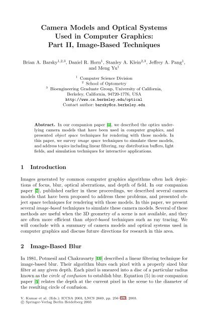
Camera Models and Optical SystemsUsed in Computer Graphics:Part II, Image-Based TechniquesBrian A. Barsky 1,2,3 ,DanielR.Horn 1 , Stanley A. Klein 2,3 ,JeffreyA.Pang 1 ,and Meng Yu 11 Computer Science Division2 School of Optometry3 Bioengineering Graduate Group, University of California,Berkeley, California, 94720-1776, USAhttp://www.cs.berkeley.edu/opticalContact author: barsky@cs.berkeley.eduAbstract. In our companion paper [5], we described the optics underlyingcamera models that have been used in computer graphics, andpresented object space techniques for rendering with those models. Inthis paper, we survey image space techniques to simulate these models,and address topics including linear filtering, ray distribution buffers, lightfields, and simulation techniques for interactive applications.1 IntroductionImages generated by common computer graphics algorithms often lack depictionsof focus, blur, optical aberrations, and depth of field. In our companionpaper [5], published earlier in these proceedings, we described several cameramodels that have been proposed to address these problems, and presented objectspace techniques for rendering with those models. In this paper, we presentseveral image-based techniques to simulate these camera models. Several of thesemethods are useful when the 3D geometry of a scene is not available, and theyare often more efficient than object-based techniques such as ray tracing. Wewill conclude with a summary of camera models and optical systems used incomputer graphics and discuss future directions for research in this area.2 Image-Based BlurIn 1981, Potmesil and Chakravarty [16] described a linear filtering technique forimage-based blur. Their algorithm blurs each pixel with a properly sized blurfilter at any given depth. Each pixel is smeared into a disc of a particular radiusknown as the circle of confusion to establish blur. Equation (5) in our companionpaper [5] relates the depth at the current pixel in the scene to the diameter ofthe resulting circle of confusion.V. Kumar et al. (Eds.): ICCSA 2003, LNCS 2669, pp. 256–265, 2003.c○ Springer-Verlag Berlin Heidelberg 2003

Camera Models and Optical Systems Used in Computer Graphics: Part II 257Fig. 1. Image Based Linear Filtering used on an image with a mapped cubeand sphere. On the left, the cube appears focused, and on the right the sphereappears focused. (Courtesy of Indranil Chakravarty [16].)Each point in the circle of confusion is weighted; the function that mapslocations in this circle to weights is known as the intensity distribution function(IDF) [6, 16]. Although wave optics may be used to compute the precise IDFacross the circle of confusion as a wavy Airy disc [6], according to Chen [8],a simple uniform spread of intensity across the circle of confusion can be usedwhen the lens system is not diffraction limited or when the discretization of thepixels is too great. Smearing each pixel with the appropriate circle of confusionat its corresponding depth yields the final image.On a Prime 750 machine from the early 1980’s, a 512x512 image took between3 and 125 minutes to process depending on the size of the aperture.To speed the convolution process, Rokita [17] in 1993 presented an argumentfor approximating convolution with a large circle of confusion by using manyconvolutions with smaller circles of confusion. A number of faster 3x3 convolutionfilters can replace any single larger convolution filter. Although this doesnot result in an exact uniform-intensity circle of confusion, there is not a significantdifference to a human observer between images that are generated by therepeated application of the smaller circle and those that are generated by thesingle application of the larger circle of confusion.However, there are some deeper problems with Potmesil and Chakravarty’sstraightforward method of blurring. Blurring with different filters for pixels atdifferent depths results in brightening and has artifacts arising from blurredbackground objects bleeding into focused foreground objects. When processingan image with a blurred white background and a sharp black foreground object,the final image will be dramatically brighter near the border of the black objectas in Figure 4. This effect distorts the colors of the original image, and engendershalos around sharp objects.The problem stems from the larger issues surrounding occlusion. A lens witha finite aperture allows a camera to view more of the scene than does a pinholecamera as shown in Figure 2, and thus it allows rays from behind an occludedobject to arrive at the image plane. However, Potmesil and Chakravarty’s algorithmonly obtains colors that were present in the original pinhole rendering,and never determines whether a color that was originally occluded is required.

258 B.A. Barsky et al.OccludedObjectRay through pinholeRay throughfinite apertureRay through pinholeOccludingObjectRay throughfinite apertureAperturefilmplaneFig. 2. An object that would be occluded in a scene ray traced through a pinholeappears through a finite aperture.3 Ray Distribution BufferIn [18], Shinya proposed a workaround for the inherent occlusion problem. Thistechnique computes the final color of each pixel as an average of the colorsdeposited by rays entering the lens system from all angles and striking thatpixel. For each pixel, the color values used in this computation are stored in abank of memory known as the Ray Distribution Buffer (RDB).Distributed raysPixelRDBDirection vectorScreenFig. 3. Each pixel has a sub-pixel Ray Distribution Buffer. An exit directionvector can be calculated for each sub-pixel. (Courtesy of Mikio Shinya. Adaptedfrom [18].)Shinya’s method comprises four stages: First, the image is rendered conventionallywith a depth buffer.The second stage allocates memory for the RDB for each pixel. This memoryis filled with many copies of the depth and color of the corresponding pixel in theconventionally rendered image. It is desirable to have rays spreading uniformlyacross the lens aperture. To achieve this, a direction vector is defined for each ofthese rays. Each direction vector is stored in an element of the RDB. In a givenpixel’s RDB, the set of all such direction vectors sprinkles uniformly across thelens aperture.In the third stage, at each pixel p of the image, the size of the circle of confusionfor that pixel is calculated using equation (5) in our companion paper [5].Then, in the initial image rendered in the first stage, each pixel q p contained

Camera Models and Optical Systems Used in Computer Graphics: Part II 259Fig. 4. A focused black line occludes a defocused book. Left: The standard linearfiltering method results in a translucent occluding object, which is incorrect inthis scene. Right: The occlusion problem is solved using the RDB, and the blackline is properly opaque. (Courtesy of Mikio Shinya [18].)inside the pixel p’s circle of confusion is examined. The direction of the rayemerging from each pixel q p in the pinhole rendering is calculated; that directionis compared with the directions in the pixel p’s RDB, and the correspondingmemory slot is located. The depth value in the pixel p’s RDB is compared withthe pixel q p ’s depth value and the lower depth value with its associated color isselected.After this process is repeated for each pixel, the fourth stage of the algorithmaverages the colors of the RDB into the final pixel color. This method successfullyovercomes many of the problems with Potmesil and Chakravarty’s simplerapproach, and the difference is illustrated in Figure 4. Shinya’s method requiresbetween 155 and 213 seconds on a 150 MHz IRIS Crimson R4400 depending onthe size of the circle of confusion on the majority of the image, as compared with1321 seconds for the linear filtering method [18].4 Blurring by Discrete DepthBarsky et al. [2, 3] developed a method that blurs a scene with precise opticsto produce a realistic final image. The method divides a scene into many slices,each slice containing pixels that share the same distance to the camera. Then itblurs each slice of the scene separately, with the appropriate level of blur. Finallythe slices are combined for the final image.The algorithm begins by separating the scene into discrete slices, accordingto distance from the camera. Note that both size and blur are not linear indistance, but they are approximately linear in diopters. Thus, the slices are notpositioned to be equally spaced in depth but rather they are located in equaldioptric increments, ranging from the nearest depth of interest to the farthest.The use of a scale that is linear in diopters ensures that blur will changelinearly with the number of depth filters so that large distances are not coveredwith superfluous blur filters nor a paucity of them.Humans can discriminate a change of approximately 1/8 diopter under optimalconditions; therefore, pixels within a slice may share a level of blur. Eachslice is thus blurred with a single blur filter, calculated from the IDF as describedin Section 2. Fast Fourier Transforms can be used in a relatively efficient methodfor blurring a slice.

260 B.A. Barsky et al.Fig. 5. Image-based blurring by discrete depths [2, 3]. In the left image theforeground is in focus with the background blurred, and in the right image thebackground is in focus with the foreground blurred.Additionally, Barsky et al. [4] developed an alternate mechanism to obtainan IDF by measuring a physical optical system. An instrument that measuresthe path of light directed through an optical system is used to construct an IDFfor any given collection of lenses or a patient’s eye.After each slice has been blurred, they are composited. To handle discontinuitiesbetween the blur filters at different depths, linear interpolation betweenthe two resulting images is used to eliminate sharp transitions between depthfilters.The algorithm requires 156 seconds to compute blur across 11 depth slices forthe teapot image in Figure 5 on a Apple G3 600 MHz iBook, which is significantlyfaster than distributed ray tracing on modern hardware.5 Light Field TechniquesLight field rendering [13] and lumigraph systems [9] are alternative general methodsto represent the visual information in a scene from a collection of referenceimages. Both techniques were proposed in 1996, and they share a similar structuralrepresentation of rays. Unlike model-based rendering, which uses the geometryand surface characteristics of objects to construct images, light field rendering,as an example of image-based rendering techniques, resamples an arrayof the reference images taken from different positions and generates new viewsof the scene. These images may be rendered or captured from real scenes.In 1995, McMillan and Bishop [15] proposed plenoptic modeling, based on theplenoptic function, which was introduced by Adelson and Bergen [1]. A plenopticfunction is a five-dimensional function that describes the entire view from agiven point in space. The five dimensions comprise three parameters indicatingthe position of the point, as well as a vertical and horizontal angle indicatingthe direction of the ray from the particular point. Originally, the function alsocontained wavelength and time variables. Treating time as constant and lightas monochromatic, the modeling ignores these two parameters. A light field,described by Levoy and Hanrahan [13], is a 4D reduced version of the plenoptic

Camera Models and Optical Systems Used in Computer Graphics: Part II 261vtL(u, v, s, t)uentrance planesexit planeFig. 6. 4D light field point. (Courtesy of Marc S. Levoy. Adapted from [13] c○1996 ACM, Inc. Reprinted by permission.)function. Light field rendering assumes the radiance does not change along aline. Lines are parameterized by two coordinates of intersections of the lines oneach of two parallel planes in arbitrary positions: the entrance plane and theexit plane. Figure 6 illustrates this parameterization. The system takes as inputan array of 2D images and constructs a 4D light field representation. It regardsthe camera plane and the focal plane as the entrance and exit planes of thetwo-plane parameterization, respectively. Each image is taken from a particularpoint on the camera plane and stored in a 2D array (Figure 7). Thus, the lightfield is the composition of the slices of the 2D images. Once the light field isgenerated, the system can render a new image by projecting the light field ontothe image plane, given a camera position and its orientation.One of the major challenges of this technique is to sample the light field.Since the light field is discrete, only rays from the reference images are available.When resampling the light field to form a new image, we must approximaterays that are absent from the input images. This approximation may introduceartifacts. Different methods have been suggested for interpolating rays to addressthe problem. There is also some research focusing on computing the minimumsampling rate of the light field required to reduce the artifacts, such as Lin etal. [14] and Chai et al. [7]. Levoy et al.’s approach to interpolate a ray combinesthe rays that are close to the desired ray using a 4D low pass filter. However,this integration of rays is based on the assumption that the entire scene lies ona single and fixed exit plane. Therefore, a scene that has a large range of depthwill appear blurred.The lumigraph system, which was introduced by Gortler et al. [9], proposeda different approach to reduce the artifacts arising from the sampling problem.In the algorithm, the light field is alternatively called the lumigraph. The systemfirst approximates the depth information of the scene. Next, instead of using asingle exit plane as is the case in Levoy et al. [13], the lumigraph constructs a setof exit planes at the intersections of the rays and the objects, and then projectsthe rays to the corresponding planes. A basis function based on the depth informationis associated with each 4D grid point in the light field. The color value ofthe desired ray is a linear combination of the color values of the nearby 4D pointsweighted by the corresponding basis functions. The lumigraph system reducesthe artifacts by applying depth information; however, such information can bedifficult to acquire from images captured from real scenes.

262 B.A. Barsky et al.Fig. 7. The visualization of a light field. Each image in the array represents therays arriving at one point on the camera plane from all points on the focal plane,as shown at left. (Courtesy of Marc S. Levoy. Adapted from [13] c○ 1996 ACM,Inc. Reprinted by permission.)Fig. 8. Isaksen’s parameterization uses a camera surface C, a collection of datacameras D s,t and a dynamic focal surface F .Eachray(s, t, u, v) intersects thefocal surface F at (f,g) F and is therefore named (s, t, u, v) F .(CourtesyofAaronIsaksen. Adapted from [11].)In 2000, Isaksen [11, 12] developed the dynamically reparameterized lightfield. This technique extended the light field and lumigraph rendering methods toenable a variety of aperture sizes and focus settings without requiring geometricinformation of the scene. The system associates each point on the camera planewith a small camera, called a data camera (Figure 8). A image is taken fromeach data camera at the corresponding point. To reconstruct a ray in the lightfield, the system maps a point on the focal surface onto several data cameras.This results in a ray for each selected data camera for the corresponding pointon the focal surface. A mapping function is defined to decide through which datacameras the rays pass. Then the system applies a filter to combine the values ofthe rays from all data cameras. To vary the aperture sizes, the system changes theshape of the aperture filter. This changes the number of data cameras throughwhich the rays pass. The aperture filter is also used to apply depth information.

Camera Models and Optical Systems Used in Computer Graphics: Part II 263Fig. 9. By changing the shape of the focal surface, the same image can be renderedwith varying parts in focus. (Courtesy of Aaron Isaksen [11].)The rays from several data cameras pass through the aperture and intersect onthe focal surface. If the intersection is near the surface of the virtual object, theray will appear in focus; otherwise, it will not. On the other hand, the range ofthe depth of field is limited by the number of data cameras on the camera surface.A deeper scene requires more data cameras on the camera surface. Similar tovarying aperture sizes, the system changes the focal surface dynamically. Thesampling results in the same view of the scene with different focus, dependingon which focal surface is chosen. Figure 9 shows the results of the same image,rendered with different focal surfaces. The light field input images are capturedby an Electrim EDC1000E CCD camera. Then, the new images are rendered byPC rasterizers for Direct3D 7. The real-time renderer allows users to change thelocation of the camera and the focal plane, and the aperture size in real time.An important advantage of light field rendering techniques is the capabilityof generating images without a geometric representation. Instead, the geometricinformation is implicitly obtained from a series of reference images, taken fromthe surrounding environment. Furthermore, rather than simply mapping rays topixel colors, these techniques map rays to rays and apply a prefiltering process,which integrates over collections of nearby rays.6 Realistic Lens Modeling in Interactive ComputerGraphicsHeidrich et al. [10] introduced an image-based lens model, which represents raysas a light field and maps slices of the scene light field into corresponding slicesof the camera light field, instead of using ray tracing. This technique simulatesthe aberration of a real lens and achieves hardware acceleration at the sametime. The model describes a lens as a transformation of the scene light field infront of the lens into the camera light field between the lens and the film. Dueto the aberration of the lens, rays from a grid on the film do not intersect ina single point on the image-sided surface of the lens system. In this case, themapping cannot be described as a single perspective projection. A virtual centerof projection (COP) is approximated for each grid on the film. The system

264 B.A. Barsky et al.calculates the angle between the original rays and those generated by the perspectivetransformation through the corresponding calculated virtual COP. Ifthe angle is small enough, the system continues the approximation on the nextgrid; otherwise, the grid is subdivided and the system calculates a virtual centerof projection and repeats the same process for each subgrid. Eventually, all slicesof the camera light field, are combined with weights relative to the radiometryof the incoming rays to form the final image. In addition to realistic modeling ofthe lens, another important contribution of this technique is its application ininteractive computer graphics. Light fields, which are composed of 2D images,can be easily generated by computer graphics hardware at high speeds. Oncethe light field is sampled, a final image is ready to be rendered. Heidrich’s experimentsgenerate images on a RealityEngine2 using 10 sample points on thelens with approximately 14 frames per second. The grid size on the film plane is10 x 10 polygons.7 Summary and Future DirectionsThis paper covered the theory underlying lens systems that add realistic visionand camera effects to a scene. There are both object space and image spacetechniques, and they have different tradeoffs with respect to blur quality, speed,and realism. Future directions of research may involve extending Potmesil andChakravarty’s technique to improve object identification and occlusion detectionwhen adding blur to a prerendered image. Likewise, modifying Heidrich et al.’stechnique for rendering a lens with arbitrary geometry would result in a significantlyfaster technique for rendering fish-eye distortions and other distortionsthat cannot be approximated with a thick lens. Other directions of future researchcould include automatically determining how many rays or lens samplepoints are necessary for a given image quality in the Kolb et al. and Heidrich etal. techniques, respectively.AcknowledgmentsThe authors would like to thank Adam W. Bargteil, Billy P. Chen, Shlomo(Steven) J. Gortler, Aaron Isaksen, and Marc S. Levoy for their useful discussionsas well as Mikio Shinya and Wolfgang Heidrich for providing figures.References[1] E.H. Adelson and J.R. Bergen. Computational Models of Visual Processing. TheMIT Press, Cambridge, Mass., 1991.[2] Brian A. Barsky, Adam W. Bargteil, Daniel D. Garcia, and Stanley A. Klein.Introducing vision-realistic rendering. In Paul Debevec and Simon Gibson, editors,Eurographics Rendering Workshop, pages 26–28, Pisa, June 2002.[3] Brian A. Barsky, Adam W. Bargteil, and Stanley A. Klein. Vision realistic rendering.Submitted for publication, 2003.

Camera Models and Optical Systems Used in Computer Graphics: Part II 265[4] Brian A. Barsky, Billy P. Chen, Alexander C. Berg, Maxence Moutet, Daniel D.Garcia, and Stanley A. Klein. Incorporating camera models, ocular models, andactual patient eye data for photo-realistic and vision-realistic rendering. Submittedfor publication, 2003.[5] Brian A. Barsky, Daniel R. Horn, Stanley A. Klein, Jeffrey A. Pang, and MengYu. Camera models and optical systems used in computer graphics: Part I, Objectbased techniques. In Proceedings of the 2003 International Conference on ComputationalScience and its Applications (ICCSA’03), Montréal, May 18–21 2003.Second International Workshop on Computer Graphics and Geometric Modeling(CGGM’2003), Springer-Verlag Lecture Notes in Computer Science (LNCS),Berlin/Heidelberg. (These proceedings).[6] Max Born and Emil Wolf. Principles of Optics. Cambridge University Press,Cambridge, 7th edition, 1980.[7] Jin-Xiang Chai, Xin Tong, and Shing-Chow Chan. Plenoptic sampling. In KurtAkeley, editor, Proceedings of ACM SIGGRAPH 2000, pages 307–318, New Orleans,July 23–28 2000.[8] Yong C. Chen. Lens effect on synthetic image generation based on light particletheory. The Visual Computer, 3(3):125–136, October 1987.[9] Steven J. Gortler, Radek Grzeszczuk, Richard Szeliski, and Michael F. Cohen.The lumigraph. In Holly Rushmeier, editor, ACM SIGGRAPH 1996 ConferenceProceedings, pages 43–54, New Orleans, August 4–9 1996.[10] Wolfgang Heidrich, Philipp Slusallek, and Hans-Peter Seidel. An image-basedmodel for realistic lens systems in interactive computer graphics. In Wayne A.Davis, Marilyn Mantei, and R. Victor Klassen, editors, Proceedings of GraphicsInterface 1997, pages 68–75. Canadian Human Computer Communication Society,May 1997.[11] Aaron Isaksen. Dynamically reparameterized light fields. Master’s thesis, Departmentof Electrical Engineering and Computer Science, Massachusetts Institute ofTechnology, Cambridge, Mass., November 2000.[12] Aaron Isaksen, Leonard McMillan, and Steven J. Gortler. Dynamically reparameterizedlight fields. In Kurt Akeley, editor, Proceedings of ACM SIGGRAPH 2000,pages 297–306, New Orleans, July 23–28 2000.[13] Marc Levoy and Pat Hanrahan. Light field rendering. In Holly Rushmeier, editor,ACM SIGGRAPH 1996 Conference Proceedings, pages 31–42, New Orleans,August 4–9 1996.[14] Zhouchen Lin and Heung-Yeung Shum. On the numbers of samples needed inlight field rendering with constant-depth assumption. In Computer Vision andPattern Recognition 2000 Conference Proceedings, pages 588–579, Hilton HeadIsland, South Carolina, June 13–15 2000.[15] Leonard McMillan and Gary Bishop. Plenoptic modeling: An image-based renderingsystem. In ACM SIGGRAPH 1995 Conference Proceedings, pages 39–46,Los Angeles, August 6–11 1995.[16] Michael Potmesil and Indranil Chakravarty. Synthetic image generation with alens and aperture camera model. ACM Transactions on Graphics, 1(2):85–108,April 1982. (Original version in ACM SIGGRAPH 1981 Conference Proceedings,Aug. 1981, pp. 297-305).[17] Przemyslaw Rokita. Fast generation of depth-of-field effects in computer graphics.Computers & Graphics, 17(5):593–595, September 1993.[18] Mikio Shinya. Post-filtering for depth of field simulation with ray distributionbuffer. In Proceedings of Graphics Interface ’94, pages 59–66, Banff, Alberta,May 1994. Canadian Information Processing Society.