Valuation of Barrier Options in a Black Scholes Setup with Jump Risk
Valuation of Barrier Options in a Black Scholes Setup with Jump Risk
Valuation of Barrier Options in a Black Scholes Setup with Jump Risk

You also want an ePaper? Increase the reach of your titles
YUMPU automatically turns print PDFs into web optimized ePapers that Google loves.
Discussion Paper No. B{446<br />
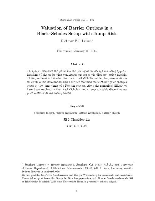
<strong>Valuation</strong> <strong>of</strong> <strong>Barrier</strong> <strong>Options</strong> <strong>in</strong> a<br />
<strong>Black</strong>{<strong>Scholes</strong> <strong>Setup</strong> <strong>with</strong> <strong>Jump</strong> <strong>Risk</strong><br />
Dietmar P.J. Leisen <br />
This version: January 12, 1999.<br />
Abstract<br />
This paper discusses the pitfalls <strong>in</strong> the pric<strong>in</strong>g <strong>of</strong> barrier options us<strong>in</strong>g approximations<br />
<strong>of</strong> the underly<strong>in</strong>g cont<strong>in</strong>uous processes via discrete lattice models.<br />
These problems are studied rst <strong>in</strong> a <strong>Black</strong>{<strong>Scholes</strong> model. Improvements result<br />
from a tr<strong>in</strong>omial model and a further modied model where price changes<br />
occur at the jump times <strong>of</strong> a Poisson process. After the numerical diculties<br />
have been resolved <strong>in</strong> the <strong>Black</strong>{<strong>Scholes</strong> model, unpredictable discont<strong>in</strong>uous<br />
price movements are <strong>in</strong>corporated.<br />
Keywords<br />
b<strong>in</strong>omial model, option valuation, lattice{approach, barrier option<br />
JEL Classication<br />
C63, G12, G13<br />
<br />
Stanford University, Hoover Institution, Stanford, CA 94305, U.S.A., and University<br />
<strong>of</strong> Bonn, Department <strong>of</strong> Statistics, Adenauerallee 24{42, 53113 Bonn, Germany, email:<br />
leisen@hoover.stanford.edu<br />
We are grateful to Dieter Sondermann and Holger Wiesenberg for comments and assistance.<br />
F<strong>in</strong>ancial support from the Deutsche Forschungsgeme<strong>in</strong>schaft, Sonderforschungsbereich 303<br />
at Rhe<strong>in</strong>ische Friedrich-Wilhelms-Universitat Bonn is gratefully acknowledged.<br />
1
1 Introduction<br />
Over time, barrier options have become <strong>in</strong>creas<strong>in</strong>gly popular to reduce the<br />
cost <strong>of</strong> pla<strong>in</strong> vanilla options while <strong>in</strong>corporat<strong>in</strong>g <strong>in</strong>dividual views <strong>of</strong> market<br />
participants concern<strong>in</strong>g the asset evolution <strong>in</strong> an easy way: the payo <strong>of</strong> barrier<br />
options depends on whether the asset price path will (not) cross a prespecied<br />
boundary. Of course, similar to standard options, they are also used to <strong>in</strong>sure<br />
aga<strong>in</strong>st price drops below the barrier. Standard barrier options do then either<br />
pay o a call or a put at the maturity date. For all these eight standard barrier<br />
options <strong>with</strong> s<strong>in</strong>gle barrier, closed form solutions are available <strong>in</strong> the <strong>Black</strong>{<br />
<strong>Scholes</strong> setup (see Rub<strong>in</strong>ste<strong>in</strong> and Re<strong>in</strong>er (1991) and Carr (1995)). For double<br />
barrier options, however, analytical approximations are known only <strong>in</strong> some<br />
specic cases (see Kunitomo and Ikeda (1992)). Numerical procedures have to<br />
be applied to come up <strong>with</strong> prices, especially <strong>in</strong> those generalizations <strong>of</strong> the<br />
<strong>Black</strong>{<strong>Scholes</strong> setup, <strong>in</strong> which jumps are possible.<br />
In this paper we are <strong>in</strong>terested <strong>in</strong> the \ecient" pric<strong>in</strong>g <strong>of</strong> barrier options us<strong>in</strong>g<br />
approximations <strong>of</strong> the underly<strong>in</strong>g process. It is well known that b<strong>in</strong>omial<br />
models suer from numerical deciencies <strong>with</strong> barrier options: <strong>in</strong>creas<strong>in</strong>g the<br />
renement, prices converge erratically <strong>in</strong> a saw{tooth manner to the cont<strong>in</strong>uous<br />
time price and even high renements do not ensure adequate accuracy.<br />
Many authors addressed this problem and suggested adjustments. Ritchken<br />
(1995), and Cheuk and Vorst (1996) constructed trees where the nodes lie on<br />
the barrier. Figlewski and Gao (1998) rene the tree further at the barrier.<br />
Our improvements are related to the nite dierence approach (see Boyle and<br />
Tian (1998)): we start from a discretization <strong>of</strong> the asset space, <strong>in</strong>stead <strong>of</strong> discretiz<strong>in</strong>g<br />
time rst, as previous approaches did. With barrier options this is a<br />
straightforward way to have nodes on critical levels by construction. We recover<br />
b<strong>in</strong>omial models <strong>with</strong> the specic renement<strong>of</strong>Boyle and Lau (1994). To<br />
<strong>in</strong>corporate our approach <strong>in</strong> full generality we make use <strong>of</strong> tr<strong>in</strong>omial models.<br />
S<strong>in</strong>ce discretiz<strong>in</strong>g the asset space breaks up the time discretization, we allow<br />
for random trad<strong>in</strong>g, similar to Leisen (1998b) for American put options,<br />
and Rogers and Stapleton (1998) for barrier options. However, the latter did<br />
not recognize the numerical deciencies result<strong>in</strong>g from the strike at maturity,<br />
which will be prevented <strong>in</strong> our tr<strong>in</strong>omial model. We also dier from their<br />
approach by assum<strong>in</strong>g that trad<strong>in</strong>g dates are the jump times <strong>of</strong> a Poisson<br />
process, which results <strong>in</strong> simple valuation formulas. Our parameters are set<br />
<strong>in</strong> accordance <strong>with</strong> a convergence theorem <strong>of</strong> the processes which also ensures<br />
convergence <strong>of</strong> prices. The model smoothes the convergence structure<br />
even better. The order <strong>of</strong> convergence <strong>in</strong>creases from 1=2 to 1 and removes<br />
the wavy patterns. Us<strong>in</strong>g extrapolation we are able to obta<strong>in</strong> even quadratic<br />
order.<br />
2
After the numerical deciencies have been removed <strong>in</strong> the <strong>Black</strong>{<strong>Scholes</strong> setup,<br />
we turn to the framework <strong>of</strong> Merton (1976), add<strong>in</strong>g a compound Poisson process<br />
to the <strong>Black</strong>{<strong>Scholes</strong> model. This models the empirical observation <strong>of</strong><br />
sudden strong price changes. An extension <strong>of</strong> b<strong>in</strong>omial models to this setup<br />
was proposed by Am<strong>in</strong> (1993), which unfortunately <strong>in</strong>herits from there its<br />
poor convergence properties, especially <strong>with</strong> barrier options. Our model <strong>with</strong><br />
random jump times driven by a Poisson process allows us <strong>in</strong> a simple way<br />
and <strong>in</strong>tuitive way to <strong>in</strong>corporate jumps. It <strong>in</strong>herits the extraord<strong>in</strong>ary convergence<br />
properties from the tr<strong>in</strong>omial model <strong>in</strong> its randomized version. Aga<strong>in</strong>,<br />
a theorem ensures convergence to the cont<strong>in</strong>uous time solution.<br />
The rema<strong>in</strong>der <strong>of</strong> the paper is organized as follows. In section 2 we present the<br />
jump{diusion setup as well as the barrier option contract. Section 3 expla<strong>in</strong>s<br />
the pitfalls <strong>in</strong> discretiz<strong>in</strong>g accord<strong>in</strong>g to CRR. In section 4 these diculties are<br />
circumvented us<strong>in</strong>g a suitable tr<strong>in</strong>omial model. This model is then randomized.<br />
Section 5 <strong>in</strong>corporates \strong" jumps. Section 6 discusses barrier option<br />
valuation and the price accuracy <strong>in</strong> our framework. Section 7 concludes the<br />
paper.<br />
2 The <strong>Setup</strong><br />
On a probability space (; F;P) we study an economy (B;S), consist<strong>in</strong>g <strong>of</strong><br />
the Bond B and the stock S. The <strong>in</strong>terest rate r is assumed to be constant over<br />
time (B t = expfrtg) and the stock price evolves under the objective measure<br />
P accord<strong>in</strong>g to<br />
S t = S 0 G t J t ; (1)<br />
where G t = expft + W t g ; (2)<br />
and J t =<br />
YN t<br />
i=1<br />
V i : (3)<br />
(N t ) t isaPoisson process <strong>with</strong> constant parameter , (V i ) i a sequence <strong>of</strong> non{<br />
negative iid random variables, 2 IR, 2 IR + .<br />
The process (G t ) t is the cont<strong>in</strong>uous process known as geometric Brownian<br />
motion and has stationary, Gaussian returns. It was suggested by Samuelson<br />
(1965) to model the evolution <strong>of</strong> a stock. S<strong>in</strong>ce <strong>Black</strong> and <strong>Scholes</strong> (1973) it is<br />
used as one <strong>of</strong> the standard nancial models. S evolves accord<strong>in</strong>g to G until<br />
the next jump time <strong>of</strong> the Poisson process at which N changes from, say,<br />
i to i +1.We then observe a per{cent change V i , 1, i.e., the stock changes<br />
value from S , before the jump to S , V i .<br />
3
So, the two parts can be <strong>in</strong>terpreted as follows: (G t ) t models the \typical"<br />
evolution <strong>of</strong> the stock under the \normal" arrival <strong>of</strong> <strong>in</strong>formation, whereas<br />
(J t ) t models jumps <strong>in</strong> the stock prices, due to some rare strong <strong>in</strong>formation<br />
shock. S<strong>in</strong>ce the Poisson process is \memoryless," the expected time until<br />
the next shock occurs is equal to 1=, <strong>in</strong>dependent <strong>of</strong> current time. Merton<br />
(1976) studied this model under the assumptions that the (V i ) i are lognormally<br />
distributed random variables and and (N t ) t are specic for the rm under<br />
consideration.<br />
The <strong>Black</strong>{<strong>Scholes</strong> setup is a so{called complete market, i.e., any cont<strong>in</strong>gent<br />
claim on the stock can be hedged (see Due (1992)). The no{arbitrage pr<strong>in</strong>ciple<br />
is sucient to price any claim. In the language <strong>of</strong> Harrison and Kreps<br />
(1979) this means that there is a probability measure Q, equivalent to P ,<br />
and under which (G t =B t ) t is a mart<strong>in</strong>gale. Such a measure gives rise to a<br />
l<strong>in</strong>ear pric<strong>in</strong>g operator; it is completely specied for the (B;G) market by<br />
G = r , 2 =2.<br />
In our setup, however, we are <strong>in</strong> an <strong>in</strong>complete market; the unforeseeable jump<br />
can not hedged. Under the assumption <strong>of</strong> no{arbitrage there isamultiplicity<br />
<strong>of</strong> equivalent mart<strong>in</strong>gale measure (EMM) under which agents do evaluate this<br />
risk. The mathematical nance literature suggests the use specic EMM, derived<br />
from hedg<strong>in</strong>g criteria (see Follmer and Sondermann (1986) and Follmer<br />
and Schweizer (1991)). When our setup is used to model \market crashes,"<br />
i.e., (J t ) t represents jumps <strong>in</strong> the aggregate or market portfolio, the procedure<br />
taken <strong>in</strong> the mathematical nance literature seems appropriate. If the<br />
asset (J t ) t would be traded <strong>in</strong> the market, the three assets (B; S; J) would<br />
constitute a complete market. As it is, however, not traded, under the EMM<br />
Q chosen by the market for valuation, only (S t ) t has to be a mart<strong>in</strong>gale, but<br />
(J t ) t not; the description <strong>of</strong> (J t ) t (under P ) and the choice <strong>of</strong> Q together <strong>with</strong><br />
the Girsanov{Theorem are equivalent. Our view on this is that <strong>of</strong> specify<strong>in</strong>g<br />
under an appropriate measure the process (J t ) t by<br />
J t = J 0 e (,E[V i,1])t<br />
YN t<br />
i=1<br />
V i ; (4)<br />
for some 2 IR, which will be expla<strong>in</strong>ed below. Us<strong>in</strong>g the description <strong>of</strong> the<br />
stochastic exponential we derive E[J t =J 0 ] = e t (see Protter (1990) or Jacod<br />
and Shiryaev (1987)). Us<strong>in</strong>g the Girsanov{Theorem as <strong>in</strong> the <strong>Black</strong>{<strong>Scholes</strong><br />
setup gives then the EMM for the (B; S; J) market as a change <strong>in</strong> the Wiener<br />
measure for which S = r , 2 =2 , . For a detailed discussion, we refer to<br />
Wiesenberg (1998).<br />
Then ~ =lnE[J t =J 0 ]=t , r = , r can be <strong>in</strong>terpreted as the excess return on<br />
the risky process (J t ) t over the riskless rate. With exogenously xed parameters<br />
and (V i ), species the risk{premium. As this is a \free" parameter,<br />
4
we can treat the choice problem <strong>of</strong> an EMM as the specication problem <strong>of</strong><br />
an appropriate risk{premium <strong>in</strong> the market. Hamilton (1995), Bates (1996),<br />
and Trautmann and Be<strong>in</strong>ert (1995) discussed the implementation, i.e., how to<br />
<strong>in</strong>fer the properties <strong>of</strong> the jump component (J t ) t <strong>in</strong> the stock process (S t ) t .<br />
Similar to Merton (1976) we are <strong>in</strong>terested <strong>in</strong> the case where jumps are rm<br />
specic, and therefore uncorrelated <strong>with</strong> the market as a whole. In the sense<br />
<strong>of</strong> the CAPM this is non systematic risk, has a <strong>of</strong> zero and therefore the<br />
premium is zero. Bates (1996) gives statistical evidence that the risk premium<br />
is non{zero, i.e., the jump{risk is correlated to the market as a whole, and<br />
\crashes" need to be taken <strong>in</strong>to account. However we use the Merton (1976)<br />
model as a start<strong>in</strong>g po<strong>in</strong>t for our presentation; our approach is general and can<br />
easily be generalized to a non{zero . Section 6 studies numerical simulations<br />
<strong>in</strong> the case <strong>of</strong> a rm allow<strong>in</strong>g for ru<strong>in</strong> (V i 0).<br />
<strong>Barrier</strong> options are a type <strong>of</strong> exotic options where the payo depends on the<br />
cross<strong>in</strong>g <strong>of</strong> predeterm<strong>in</strong>ed levels, which may be either discretely or cont<strong>in</strong>uously<br />
monitored. In the event <strong>of</strong> a cross<strong>in</strong>g, depend<strong>in</strong>g on the specication, a<br />
lump{sum (called \rebate") might bepayed, another asset might be activated<br />
(called \knock{<strong>in</strong>") or deactivated (\knock{out"). Typical examples are those<br />
where the secondary asset is a pla<strong>in</strong> vanilla option, e.g., a down (up) and <strong>in</strong><br />
(out) barrier option pays this o, if some barrier H < S 0 (H > S 0 ) is (not)<br />
crossed and noth<strong>in</strong>g otherwise.<br />
We are <strong>in</strong>terested here <strong>in</strong> cont<strong>in</strong>uously monitored constant barrier options,<br />
where the nal payo is that <strong>of</strong> a pla<strong>in</strong> vanilla European option. We explicitly<br />
allow for multiple barrier options. The barrier option payo depends on a<br />
\choice variable" as follows: The set conta<strong>in</strong>s all those paths !, where the<br />
term<strong>in</strong>al payo will be activated. Then the term<strong>in</strong>al payo is 1 !2 f(S T ), where<br />
f is the payo function at maturity, and its price is E h e ,rT 1 !2 f(S T ) i .<br />
3 B<strong>in</strong>omial Pitfalls<br />
This section studies the numerical deciencies <strong>with</strong> barrier option pric<strong>in</strong>g <strong>in</strong><br />
the <strong>Black</strong>{<strong>Scholes</strong> setup, i.e., the model S t = S 0 G t , us<strong>in</strong>g b<strong>in</strong>omial models.<br />
Start<strong>in</strong>g <strong>with</strong> CRR many authors presented so called b<strong>in</strong>omial models for the<br />
asset evolution. We recall here briey the CRR model to present the ma<strong>in</strong><br />
diculties. The specication <strong>of</strong> a renement n <strong>of</strong> the time axis [0;T] yields a<br />
discretization set T n = f0 =t n;0
node, i.e., we model the (per{period) return by<br />
R n;i <br />
and the stock process by<br />
8<br />
><<br />
>:<br />
+x n ; q n<br />
,x n ;1, q n<br />
; (5)<br />
<strong>with</strong><br />
tY<br />
N (n)<br />
G (n)<br />
t<br />
:= R n;i ; (6)<br />
i=1<br />
t<br />
<br />
N (n)<br />
t := : (7)<br />
t n<br />
Let us denote by X t = ln G t (X (n)<br />
t<br />
= ln G (n)<br />
t<br />
) the (discrete) logarithmic process.<br />
To match the cont<strong>in</strong>uous per{period variance, we set<br />
x n = <br />
q<br />
t n : (8)<br />
For pric<strong>in</strong>g, only the evolution <strong>of</strong> the processes under the risk{neutral probability<br />
measures Q (n) matters. It corresponds here to the risk{neutral probability<br />
Q (n) <strong>of</strong> the cont<strong>in</strong>uous process, and is represented by the probability q n for an<br />
up{move, such that E[R n;1 ] = expfrt n g.<br />
h i h i<br />
Theorem 1 If E ln R n;1 = r ,<br />
2<br />
tn , then E R n;1 = expfrtn g +<br />
2<br />
O(t n ). On the other hand, h if the i mart<strong>in</strong>gale measure condition E[R n;1 ] =<br />
expfrt n g holds, then E ln R n;1 = r ,<br />
2<br />
tn + O(t 3=2<br />
n<br />
).<br />
In both cases we have S (n)<br />
d<br />
=) S.<br />
2<br />
PROOF. The condition expfrt n g = E[R n;1 ] is equivalent to<br />
1+rt n + O(t 2 n)<br />
= expfrt n g = q n exp x n +(1, q n ) exp ,x n<br />
= q n<br />
<br />
1+xn +x 2 n=2 +(1, q n ) 1 , x n +x 2 n=2 + O(t 3=2<br />
n )<br />
=1+x n (2q n , 1)+x 2 n=2+O(t 3=2<br />
which is equivalentto r , 2<br />
2<br />
n )<br />
<br />
tn =(2q n ,1) p t n +O(t 3=2)=E[ln<br />
R n<br />
n;1]+<br />
). This and the converse | which follows similarly | prove the rst<br />
O(tn<br />
3=2<br />
two assertions. Then Donsker's theorem proves X (n)<br />
concludes, observ<strong>in</strong>g that the exponential function is cont<strong>in</strong>uous.<br />
d<br />
=) X and the pro<strong>of</strong><br />
6
Accord<strong>in</strong>g to theorem 1 there are two alternative ways <strong>of</strong> specify<strong>in</strong>g q n . First,<br />
look<strong>in</strong>g at the processes G and G (n)<br />
we can match h their i risk{neutral drift<br />
E[R n;i ] = expfrt n g. Second, we can take E ln R n;1 = r ,<br />
2<br />
tn , to<br />
match the drift <strong>of</strong> the logarithmic processes X and X (n) . In the limit the same<br />
processes and thus the same prices will result. We will use the second one<br />
to specify the risk{neutral probability, and require E h R n;1<br />
i<br />
= tn , where<br />
= r , 2<br />
. Easy calculations reveal that<br />
2<br />
2<br />
q n = 1 2 + t n , n<br />
(9)<br />
2x m<br />
= 1 2 + r , q 2<br />
2<br />
t n : (10)<br />
2<br />
Figure 1 presents a pric<strong>in</strong>g example for a down{and{out call <strong>with</strong> strike<br />
8.1<br />
8<br />
CRR<br />
cont<strong>in</strong>uous price<br />
7.9<br />
7.8<br />
price<br />
7.7<br />
7.6<br />
7.5<br />
7.4<br />
7.3<br />
7.2<br />
20 40 60 80 100 120 140 160 180 200<br />
ref<strong>in</strong>ement n<br />
Fig. 1. price picture for the barrier option, depict<strong>in</strong>g the convergence structure<br />
X = 110 and a barrier at H = 90 written on a stock when today's stock price<br />
S 0 is 100, the volatilityis =0:2 and the <strong>in</strong>terest rate is r =0:1. We observe a<br />
unregular convergence to the cont<strong>in</strong>uous time solution. The structure exhibits<br />
the typical \saw{tooth" pattern well known <strong>in</strong> the literature. We observe also<br />
the \odd{even ripple." Figure 2 depicts the error on a log{log scale. S<strong>in</strong>ce the<br />
function 1= p n is an appropriate upper bound<strong>in</strong>g l<strong>in</strong>e, the order <strong>of</strong> convergence<br />
is 1=2. Compared to the pric<strong>in</strong>g <strong>of</strong> pla<strong>in</strong> vanilla options, where the order is 1 we<br />
lose 1=2. We see that we have quite high errors <strong>in</strong> the worst case. Furthermore<br />
we deduce that we need at least a renement <strong>of</strong>1= p n =0:01 , n = 10000 to<br />
ensure \penny{accuracy."<br />
The convergence is slower than <strong>in</strong> a standard European call and put option<br />
case, s<strong>in</strong>ce <strong>in</strong> b<strong>in</strong>omial models the whole probability mass is concentrated <strong>in</strong><br />
7
1<br />
cont<strong>in</strong>uous price<br />
1/sqrt(n)<br />
0.1<br />
error<br />
0.01<br />
0.001<br />
0.0001<br />
10 100<br />
ref<strong>in</strong>ement n<br />
Fig. 2. error picture for the barrier option<br />
the tree{nodes. The dierence <strong>in</strong> probability between two adjacent nodes is<br />
known to be <strong>of</strong> the order O(1= p n) (see Feller (1966)). Now, if, result<strong>in</strong>g from<br />
an <strong>in</strong>crease <strong>in</strong> the renement by one, a node \jumps" over the barrier layer,<br />
tak<strong>in</strong>g the correspond<strong>in</strong>g probability mass <strong>with</strong>, we will observe a similar<br />
numerical eect. To prevent this for barrier options, Ritchken (1995) po<strong>in</strong>ted<br />
out that it has to be ensured that there lies a node exactly on the barrier for<br />
any renement. We characterize all (for double or even multi barrier options)<br />
barrier l<strong>in</strong>es as a \critical l<strong>in</strong>e." Similarly Boyle and Lau (1994) argued to take<br />
depend<strong>in</strong>g on m 2 IIN only the renements<br />
6<br />
4 m2 2 T<br />
<br />
ln<br />
S 0<br />
H<br />
2<br />
7 7775<br />
: (11)<br />
These renements are exactly the one's before an entire layer jumps over the<br />
barrier, aga<strong>in</strong>. Pric<strong>in</strong>g errors are reduced to a size comparable to those <strong>of</strong> call<br />
options.<br />
4 How to discretize properly<br />
This section discusses the construction <strong>of</strong> a tr<strong>in</strong>omial model <strong>in</strong> a rst approach<br />
to remove the pitfalls <strong>of</strong> the previous section. Our approach to this problem is<br />
as follows: Discretiz<strong>in</strong>g time, and then study<strong>in</strong>g the result<strong>in</strong>g X{grid, runs <strong>in</strong>to<br />
problems. We are discretiz<strong>in</strong>g the wrong th<strong>in</strong>g; the X{axis by a renement m<br />
needs to be discretized rst, yield<strong>in</strong>g x m , and then the renement n m <strong>of</strong> the<br />
t{axis should be set appropriately, rewrit<strong>in</strong>g equation (8) as<br />
8
() n m =<br />
xm<br />
2<br />
t n = :<br />
$<br />
<br />
(12)<br />
T<br />
: (13)<br />
<br />
x m<br />
2<br />
%<br />
For a down{and{out call option to place grid po<strong>in</strong>ts on the barrier H requires<br />
x m = ln S 0=H<br />
. Interest<strong>in</strong>gly, this way we recover formula (11) derived by<br />
m<br />
Boyle and Lau (1994) as the result<strong>in</strong>g renement n m <strong>in</strong> equation (13). In the<br />
symmetrical case where jS 0 , Xj = jS 0 , Hj this improves the accuracy and<br />
reduces the oscillations to a size comparable to European call options. To<br />
encounter this problem <strong>in</strong> the general case we need to ensure that nodes also<br />
lie on the strike.<br />
We will now present a rst approach to resolve this diculty <strong>in</strong> full generality.<br />
Later then, we expla<strong>in</strong> it on a concrete example. We call critical layer all<br />
barrier l<strong>in</strong>es (possibly many), the strike and the current asset price. Let us<br />
denote by L the ordered set l 1 < ::: < l L <strong>of</strong> critical layers, and by L 0 =<br />
Lnfl 1 ;l L g the <strong>in</strong>ner po<strong>in</strong>ts. First we dene variables for 0 < i < L , 1,<br />
x m;i = l i+1,l i<br />
, and then x m m;L =x m;L,1 and x m;0 =x m;1 , and for x 2<br />
[l i,1 ;l i [: x u m(x) = m;i,1 and for x 2]l i,1 ;l i ]: x d m(x) = m;i . This denes a<br />
discrete time{homogeneous grid for the stock values over time. Moreover we<br />
dene the m<strong>in</strong>imum x m = m<strong>in</strong> i x m;i <strong>of</strong> all. We model the return, depend<strong>in</strong>g<br />
on some x 2 IR, by a tr<strong>in</strong>omial random variable R m;i <strong>of</strong> the form:<br />
R m;i (x) <br />
8<br />
><<br />
>:<br />
x u m(x)<br />
; p m (x)<br />
0 ;1, p m (x) , q m (x)<br />
,x d m(x) ; q m (x)<br />
For t n ;n m dened by equation (12),(13), we call the processes<br />
: (14)<br />
N tX<br />
(m)<br />
X (m)<br />
t =<br />
G (m)<br />
t<br />
N (m)<br />
t =<br />
i=1<br />
<br />
R m;i X (n)<br />
t,<br />
(15)<br />
= exp X (n)<br />
t (16)<br />
t<br />
t m<br />
<br />
the Tr<strong>in</strong>omial Adjusted (TA) model.<br />
(17)<br />
The choice <strong>of</strong> x u m(x); x d m(x) will give us sucient degrees <strong>of</strong> freedom to<br />
place nodes on critical \l<strong>in</strong>es," like the barrier and the strike price. Here, we<br />
deal <strong>with</strong> a tr<strong>in</strong>omial model <strong>in</strong> order to get the variance right despite the<br />
complication that discretizations are not constant and change at critical l<strong>in</strong>es.<br />
The process seems to be path{dependent; however this is only conditionally<br />
9
on the actual state. It rema<strong>in</strong>s recomb<strong>in</strong><strong>in</strong>g and therefore computationally<br />
simple, as it can be handled as any standard tr<strong>in</strong>omial model for calculations.<br />
The dependence on x is easy to resolve. We will drop it <strong>in</strong> the sequel to present<br />
the ma<strong>in</strong> ideas.<br />
Let us expla<strong>in</strong> our approach <strong>in</strong> detail for a down{and{out call option <strong>in</strong> gure<br />
3 where a strike price is at X = 120 and a barrier is at H = 90. We see that<br />
6<br />
x m;3<br />
strike<br />
XXXXXXXXz<br />
x<br />
current stock XXXXXXXXz **<br />
m;2<br />
price<br />
XXXXXXXXz<br />
*<br />
x m;1<br />
barrier<br />
x m;0<br />
?<br />
t 2;0 t 2;1 t 2;2<br />
Fig. 3. Example dynamics<br />
we can dist<strong>in</strong>guish L = 3 critical layers and four dierent ranges: one below<br />
the barrier, one between the barrier and the current asset price, one between<br />
the strike and the current asset price and one above the strike. In each <strong>of</strong> the<br />
two <strong>in</strong>ner ranges we need a dierent x m . To place nodes on critical layers,<br />
we take between the barrier and the current asset price x m;1 = j ln H=S 0 j=m<br />
and between the strike and the current asset price x m;2 = j ln K=S 0 j=m.<br />
This denes our grid for the asset evolution. As there is no clear choice for<br />
x m;3 (x m;0 ), our approach takes x m;2 (x m;1 ) for simplicity. Please note<br />
that although we focus here on a down{and{out call for ease <strong>of</strong> exposition,<br />
our approach is general and can easily be generalized, e.g. to double barrier<br />
options.<br />
d<br />
A consistency requirement is G (m)<br />
=) G. S<strong>in</strong>ce the exponential function is<br />
cont<strong>in</strong>uous, this is equivalent toX (m)<br />
=) d<br />
X. So, sett<strong>in</strong>g = r , 2<br />
, accord<strong>in</strong>g<br />
2<br />
to Donsker's theorem the follow<strong>in</strong>g two conditions are sucient:<br />
and<br />
E h R m;i<br />
i<br />
t n<br />
Var h<br />
R m;i<br />
i<br />
t n<br />
n<br />
,! ; (18)<br />
n<br />
,! 2 : (19)<br />
We require them to hold <strong>with</strong> equality:<br />
10
x u mp m , x d mq m = t n ; (20)<br />
(x u m) 2 p m +(x d m) 2 q m = 2 t n ; (21)<br />
which can be resolved easily<br />
p m =<br />
<br />
x<br />
d<br />
m<br />
+ 2 <br />
tn<br />
x u m(x u m +x d m) ; (22)<br />
and<br />
q m = (,xu m<br />
+ 2 )t n<br />
x d m(x u m +x d m) : (23)<br />
Theorem 2 For suciently high renements, all probabilities p m ;q m ; 1,p m ,<br />
q m are positive and X (m)<br />
=) d<br />
X and G (m) =) d<br />
G.<br />
PROOF. Positivity <strong>of</strong> the probabilities follows from t n = (x n =) 2 , and<br />
equations (22), (23) s<strong>in</strong>ce<br />
and<br />
0 <<br />
<br />
x 2 m<br />
x u m(x u m<br />
+x d m) xm<br />
2<br />
< 1 ;<br />
<br />
<br />
x d m<br />
x u m(x u m +x d m) xm<br />
<br />
2<br />
m<br />
,! 0 :<br />
The observation that the barrier option <strong>with</strong> a put as payo{function is cont<strong>in</strong>uous<br />
and bounded, the above theorem and put{call parity ensure convergence<br />
<strong>of</strong> approximate values calculated to their cont<strong>in</strong>uous time counterpart. Please<br />
note, that this price consistency holds whenever we know that processes are<br />
consistent <strong>in</strong> the limit.<br />
Table 1 gives a pric<strong>in</strong>g example for a barrier option us<strong>in</strong>g CRR, TA, and the<br />
modied Richardson extrapolation rule (see Leisen (1998a))<br />
e m<br />
=(n m+1 m+1 , n m m )=(n m+1 , n m ) ; (24)<br />
iterat<strong>in</strong>g m = 1;::: ;8. The RT model will be <strong>in</strong>troduced <strong>in</strong> the follow<strong>in</strong>g<br />
section. Figure 4 conta<strong>in</strong>s the error picture for the same parameter constellation<br />
as <strong>in</strong> table 1. Here we take only specic renements; we see that the<br />
convergence structure is much smoother than <strong>in</strong> gure 2. However it is not suf-<br />
ciently smooth to apply extrapolation, which do therefore not depict. For TA,<br />
<strong>in</strong> comparison to CRR, errors are drastically reduced and extrapolation gives<br />
quickly \penny{accuracy." We do also observe that the convergence structure<br />
is fairly smooth.<br />
11
m n m CRR TA e TA<br />
RT e RT<br />
1 8 8.44693 7.89878 7.93419 6.60928 8.14613<br />
2 34 8.17859 7.92586 7.92367 7.78452 7.97775<br />
3 78 8.04017 7.92463 7.98542 7.89352 7.97775<br />
4 140 7.97567 7.95155 7.98644 7.93082 7.97837<br />
5 220 8.03844 7.96423 7.97371 7.94811 7.97904<br />
6 316 8.02729 7.96711 7.97778 7.95751 7.97889<br />
7 430 7.97612 7.96994 7.98570 7.96318 7.97884<br />
8 562 8.0086 7.97364 7.97786 7.96686 7.97883<br />
Table 1<br />
Pric<strong>in</strong>g example <strong>with</strong> S=100, X=110, H=85, T=1, r=0.1, =0:2. The cont<strong>in</strong>uous<br />
time price is 7.97888.<br />
10<br />
1<br />
0.1<br />
price error<br />
0.01<br />
0.001<br />
0.0001<br />
1e-05<br />
1e-06<br />
CRR<br />
TA<br />
extrapolated TA<br />
RT<br />
extrapolated RT<br />
10/n<br />
3/(n*n)<br />
10 100<br />
ref<strong>in</strong>ement n<br />
Fig. 4. error picture for the barrier option<br />
5 Randomiz<strong>in</strong>g and <strong>Jump</strong>{diusions<br />
We will now randomize the previous model. This will be an easy and straightforward<br />
way to <strong>in</strong>corporate the additional jumps whichcharacterize the jump{<br />
diusion model <strong>in</strong> dierence to the <strong>Black</strong>{<strong>Scholes</strong> setup. It turns out, <strong>in</strong> accordance<br />
to Leisen (1998b), that such a randomized model yields even better<br />
convergence results.<br />
We start <strong>with</strong> a sequence <strong>of</strong> Poisson processes N (m) =(N (m)<br />
t<br />
) t0 where N (m)<br />
t<br />
is described by<strong>in</strong>terarrival times m;i , <strong>in</strong>dependent<br />
has parameter ( m ) m . N (m)<br />
t<br />
exponentially distributed random variables <strong>with</strong> parameter 1= m and N (m)<br />
t =<br />
max fn j P n<br />
i=1<br />
m;i tg. In the previous section we approximated the process<br />
12
X between two trad<strong>in</strong>g dates t n;i ;t n;i+1 2 T n by iid random variables R m;i .<br />
Similarly here we will now approximate it by random variables R m;i between<br />
two <strong>in</strong>terarrival times m;i ; m;i+1 , which <strong>of</strong> the same form. All x m;l (l =<br />
1;::: ;L) are dened as <strong>in</strong> the last section described to place nodes on critical<br />
\l<strong>in</strong>es," like the barrier and the strike price. Then study the discrete processes<br />
X (m)<br />
t<br />
and G (m)<br />
t<br />
, dened similar to (15){(17) by<br />
N tX<br />
(m)<br />
X (m)<br />
t =<br />
G (m)<br />
t<br />
i=1<br />
R m;i ;<br />
= exp X (m)<br />
t :<br />
and we require, s<strong>in</strong>ce 1= m = E[ m;i+1 , m;i ],<br />
E h R m;i<br />
i<br />
m<br />
and Var h R m;i<br />
i<br />
m<br />
n<br />
n<br />
,! r , 2<br />
2 ; (25)<br />
,! 2 : (26)<br />
Theorem 3 Under conditions (25) and (26) we have X (m)<br />
=) d<br />
X and G (m) =)<br />
d<br />
G.<br />
PROOF. Let us dene the two sequences (depend<strong>in</strong>g on m) <strong>of</strong> processes<br />
(m)<br />
M t<br />
t <br />
and A (m)<br />
t by<br />
t<br />
and<br />
N tX<br />
(m)<br />
M (m)<br />
t =<br />
i=1<br />
A (m)<br />
t = 2 t:<br />
R m;i ,<br />
Then for each m, the processes M (m)<br />
t<br />
!<br />
r , 2<br />
t ;<br />
2<br />
t and <br />
M<br />
(m)<br />
t<br />
2<br />
<br />
(m)<br />
, A t<br />
t<br />
are mart<strong>in</strong>gales.<br />
As the jump sizes are <strong>of</strong> order x m and vanish <strong>in</strong> the limit, we deduce<br />
from the Mart<strong>in</strong>gale Central Limit Theorem as stated <strong>in</strong> Ethier and Kurtz<br />
(1986) that M =) d<br />
W. This is also sucient for G (m) =) d<br />
G, s<strong>in</strong>ce the<br />
exponential function is cont<strong>in</strong>uous.<br />
We require equations (25) and (26) to be fullled <strong>with</strong> equality, i.e.,<br />
13
(x u m) 2 p m +(x d m) 2 q m = 2<br />
m<br />
;<br />
or equivalently<br />
x u mp m , x d mq m = r , 2<br />
2<br />
m<br />
;<br />
2 + r , 2<br />
2 x<br />
u<br />
m<br />
p m =<br />
m ((x u m) 2 +x u mx d m) ;<br />
<br />
and q m = 2 , r , 2<br />
2 x<br />
d<br />
m<br />
m ((x d m) 2 +x u mx d m) :<br />
Similarly to Leisen (1998b) we take<br />
m =<br />
<br />
x m<br />
2<br />
:<br />
This choice is justied from the assumptions and s<strong>in</strong>ce E[ m;1 ]=1= m which<br />
corresponds to t n <strong>in</strong> equation (13). Then p m ;q m 2 [0; 1];p m + q m 1 which<br />
makes them feasible transition probabilities and the Poisson process N (m)<br />
is stationary, which will make valuations <strong>in</strong> the next section especially easy<br />
to perform. We call this model the Randomized Tr<strong>in</strong>omial (RT) model. The<br />
only dierence to the process studied <strong>in</strong> the last section is the driv<strong>in</strong>g process.<br />
Whereas there it was bt=t n c, here it is the Poisson process N (m)<br />
t <strong>with</strong><br />
parameter m .<br />
This model can also be used easily to construct an approximation <strong>in</strong> the jump{<br />
diusion setup. Start<strong>in</strong> <strong>with</strong> a sequence (N (m) ; R m ) m <strong>of</strong> the above type, where<br />
here = r , 2<br />
2 , E[V i , 1], we dene the process<br />
N (m) = N + N (m) ; (27)<br />
which isaPoisson process <strong>with</strong> <strong>in</strong>tensity m = + m , the sequence <strong>of</strong> random<br />
variables<br />
and the processes<br />
R 0 m;i<br />
<br />
8<br />
><<br />
>:<br />
V i ;<br />
<br />
+ m<br />
; (28)<br />
<br />
R m;i ; m<br />
+ m<br />
and<br />
N (m)<br />
tX<br />
Y (m)<br />
t =<br />
S (m)<br />
t<br />
i=1<br />
R 0 m;i ; (29)<br />
= exp Y (m)<br />
t : (30)<br />
14
The counterpart to theorem 3 is:<br />
Theorem 4 For the sequence <strong>of</strong> discrete models (Y (m) ) m dened byequations<br />
(27){(30) above we have Y (m) =) d<br />
Y and S (m) =) d<br />
S, where S is the process<br />
dened <strong>in</strong> equation (1) and Y =lnS.<br />
PROOF. Denote by h the function h : x 7! x + P N<br />
i=1<br />
U i on D. S<strong>in</strong>ce<br />
N<br />
X<br />
(m)<br />
i=1<br />
R (m)<br />
!<br />
=) d<br />
r , 2<br />
t + W t ;<br />
2<br />
and the latter is cont<strong>in</strong>uous, we conclude us<strong>in</strong>g VI.1.23 and VI.3.8 (ii) <strong>of</strong> Jacod<br />
and Shiryaev (1987):<br />
Y (m) = h<br />
0<br />
X<br />
@ N (m)<br />
R 0 A d<br />
m;i<br />
i=1<br />
1<br />
=) h r , 2<br />
2<br />
!<br />
t + W t<br />
!<br />
= Y :<br />
6 Implement<strong>in</strong>g barrier option valuation <strong>in</strong> the randomized models<br />
S<strong>in</strong>ce the structure <strong>in</strong> the randomized models diers only <strong>in</strong> the specication<br />
<strong>of</strong> the return variable, we will treat pric<strong>in</strong>g <strong>in</strong> those models for a general (R 00 m;i)<br />
which is then either (R m;i )or(R 0 m;i). The value V m <strong>of</strong> a barrier option is given<br />
by<br />
h i<br />
V m = e ,rT E 1 f(S T )<br />
<br />
= e ,rT E<br />
= e ,rT 1X<br />
n=0<br />
E[1 f(S T )jN (m)<br />
T ]<br />
<br />
E 1 f(S T )jN (m)<br />
T = n<br />
<br />
<br />
P<br />
<br />
N (m)<br />
T = n<br />
This splits up the valuation task by condition<strong>in</strong>g rst on N (m)<br />
T and then averag<strong>in</strong>g<br />
over all possible values. This is feasible, due to the <strong>in</strong>dependence <strong>of</strong><br />
N (m)<br />
and the random variables <strong>in</strong> the sequence R 00 m. Let us now denote by<br />
n the \choice variable" correspond<strong>in</strong>g to <strong>in</strong> the n{step tree <strong>with</strong> return<br />
modeled by R 00 m;i, and dene<br />
(m)<br />
n<br />
= E<br />
= E<br />
<br />
1 f(S T )jN (m)<br />
T<br />
<br />
= n<br />
<br />
1 nf(S T )jN (m)<br />
T<br />
= n<br />
<br />
:<br />
15
Therefore<br />
P 1 -<br />
PPPPPPPPPPPq<br />
S<br />
0<br />
P 1 - 1 -<br />
PPPPPPPPPPPq P PPPPPPPPPPPq<br />
(m)<br />
2 (m)<br />
2 (m)<br />
0<br />
P 1 -<br />
PPPPPPPPPPPq<br />
Fig. 5. A tr<strong>in</strong>omial grid<br />
V m = e ,(r+ m)T<br />
1X<br />
n=0<br />
( m T ) n<br />
n!<br />
(m)<br />
n<br />
(31)<br />
We cut o the <strong>in</strong>nite sum <strong>in</strong> equation (31) at an appropriate m such that<br />
lim m!1 P [N (m)<br />
T 2 f0;::: ; m g] = 1. Due to the Central Limit Theorem for<br />
renewals,<br />
N (m)<br />
T<br />
, m T<br />
q<br />
m T<br />
d<br />
=) N(0; 1) ;<br />
sett<strong>in</strong>g m =2b m T c is one appropriate choice. In the sequel we adopt as our<br />
cut{o<br />
2b mT c<br />
V m e ,(r+ m)T<br />
X<br />
n=0<br />
( m T ) n<br />
(m)<br />
n<br />
: (32)<br />
n!<br />
The value (m)<br />
n<br />
can be <strong>in</strong>terpreted as the value calculated by backward{<br />
<strong>in</strong>duction <strong>in</strong> an n{step tree grid <strong>with</strong> return (R 00 m;i) i exactly as <strong>in</strong> the CRR<br />
model, if we do not perform discount<strong>in</strong>g (see gure 5 for R 00 m;i<br />
= R m;i ). Please<br />
note that for any ~n calculat<strong>in</strong>g (m)<br />
~n gives us (m)<br />
for any n n0 =0;::: ;~n as <strong>in</strong>termediate<br />
calculations. Thus we can calculate prices as <strong>in</strong>termediate calculations<br />
0<br />
<strong>in</strong> an 2b m T c step tree and comput<strong>in</strong>g prices <strong>in</strong> our model is comparable to<br />
a tr<strong>in</strong>omial model (and therefore to the CRR model) <strong>in</strong> terms <strong>of</strong> the computational<br />
burden. In order to compare both approaches properly depend<strong>in</strong>g on<br />
its complexity, we <strong>in</strong>dex calculations <strong>in</strong> the RT by 2b m T c.<br />
As expla<strong>in</strong>ed on gure 3 we adopt the discretizations x m;0 = x m;1 =<br />
j ln H=S 0 j=m and x m;2 =x m;3 = j ln K=S 0 j=m to place all nodes on critical<br />
16
m n m RT e RT<br />
RT e RT<br />
1 8 11.0891 13.6483 2.2053 0.3539<br />
2 34 13.0461 13.2948 0.2483 0.0004<br />
3 78 13.1864 13.2930 0.1080 0.0015<br />
4 140 13.2336 13.2937 0.0608 0.0008<br />
5 220 13.2555 13.2945 0.0390 0.0001<br />
6 316 13.2673 13.2943 0.0271 0.0001<br />
7 430 13.2745 13.2942 0.0200 0.0002<br />
8 562 13.2791 13.2942 0.0153 0.0002<br />
Table 2<br />
Ru<strong>in</strong> pric<strong>in</strong>g example <strong>with</strong> S=100, X=110, H=85, T=1, r=0.1, =0:2, =0:1<br />
\l<strong>in</strong>es." Table 1 presents prices and errors. We see that RT yields even better<br />
price approximations than TA. By extrapolation we get extremely accurate<br />
price approximations. This becomes even more apparent <strong>in</strong> the error picture<br />
4. We see that prices converge <strong>with</strong> order one and extrapolated prices seem<br />
to converge even <strong>with</strong> order two. Moreover we observe a ga<strong>in</strong> <strong>in</strong> accuracy by<br />
extrapolation <strong>in</strong> comparison to the extrapolated TA model.<br />
10<br />
1<br />
0.1<br />
price error<br />
0.01<br />
0.001<br />
0.0001<br />
1e-05<br />
RT<br />
extrapolated RT<br />
1/n<br />
1/(n*n)<br />
1e-06<br />
10 100<br />
ref<strong>in</strong>ement n<br />
Fig. 6. error picture for the barrier option<br />
We now discuss the accuracy <strong>in</strong> a ru<strong>in</strong> setup (V i 0) <strong>with</strong> = 0:1. Table 2<br />
and gure 6 present values calculated for this case. We also depict errors and<br />
extrapolated prices (errors) e ( e ), calculated accord<strong>in</strong>g to equation (24). We<br />
calculated 13.2944 as the price <strong>in</strong> the CRR model <strong>with</strong> a renement <strong>of</strong> 100000.<br />
This is an estimation <strong>of</strong> the cont<strong>in</strong>uous time price. In gure 2 wesaw that 1= p n<br />
was an appropriate upper bound for the error. If we assume a similar error<br />
bound here, then the error <strong>of</strong> our estimate is less than 0:0031. Here we see<br />
17
very impressively the slow convergence <strong>of</strong> the CRR model. Immediately (<strong>with</strong><br />
m =2)we fall below this level. We do not perform a graphical analysis <strong>of</strong> the<br />
order, s<strong>in</strong>ce we can not calculate suciently accurate values; iterat<strong>in</strong>g the RT<br />
higher than m = 2 to compare the accuracy is even doubtful. It is astonish<strong>in</strong>g<br />
that the remarkable convergence properties carry over from the <strong>Black</strong>{<strong>Scholes</strong><br />
setup to the jump{diusion case.<br />
7 Conclusion<br />
This paper constructs a randomized tr<strong>in</strong>omial model. This is a natural way<br />
to approximate jump{diusions. The parameters are set such as to get consistency<br />
<strong>with</strong> the cont<strong>in</strong>uous{time processes. We discuss an easy approximation<br />
to jump{diusions and how ecient numerical approximations for barrier options<br />
result <strong>in</strong> the <strong>Black</strong>{<strong>Scholes</strong> and the jump{diusion setup.<br />
References<br />
Am<strong>in</strong>, Kaushik I., <strong>Jump</strong> Diusion Option <strong>Valuation</strong> <strong>in</strong> Discrete Time, The Journal<br />
<strong>of</strong> F<strong>in</strong>ance, 1993, 43, 1833{1863.<br />
Bates, David S., Dollar <strong>Jump</strong> Fears, 1984{1992: Distributional Abnormalities<br />
Implicit <strong>in</strong> Currency Futures <strong>Options</strong>, Journal <strong>of</strong> International Money and<br />
F<strong>in</strong>ance, 1996, 15 (1), 65{93.<br />
<strong>Black</strong>, Fischer and Myron <strong>Scholes</strong>, The Pric<strong>in</strong>g <strong>of</strong> <strong>Options</strong> and Corporate Liabilities,<br />
Journal <strong>of</strong> Political Economy, 1973, 81, 637{659.<br />
Boyle, Phelim P. and Sok Hoon Lau, Bump<strong>in</strong>g up aga<strong>in</strong>st the <strong>Barrier</strong> <strong>with</strong> the<br />
B<strong>in</strong>omial Method, The Journal <strong>of</strong> Derivatives, 1994, pp. 6{15.<br />
and Yisong Tian, An explicit nite dierence approach to the pric<strong>in</strong>g <strong>of</strong> barrier<br />
options, Applied Mathematical F<strong>in</strong>ance, 1998, pp. 17{43.<br />
Carr, Peter, Two extensions to barrier option valuation, Applied Mathematical<br />
F<strong>in</strong>ance, 1995, 2, 173{209.<br />
Cheuk, Terry H.F. and Ton C.F. Vorst, Complex <strong>Barrier</strong> <strong>Options</strong>, The Journal <strong>of</strong><br />
Derivatives, 1996, 4, 8{22.<br />
Due, Darrell, Dynamic Asset Pric<strong>in</strong>g Theory, Pr<strong>in</strong>ceton University Press, 1992.<br />
Ethier, Stuart N. and Thomas Kurtz, Markov Processes: Characterization and<br />
Convergence, John Wiley & Sons, 1986.<br />
Feller, William, An Introduction to Probability Theory and Its Applications, Vol. 2,<br />
John Wiley & Sons, 1966.<br />
18
Figlewski, Stephen and B<strong>in</strong> Gao, The Adaptive Mesh Model: A New Approach to<br />
Ecient Option Pric<strong>in</strong>g, Discussion Paper, New York University Stern School<br />
<strong>of</strong> Bus<strong>in</strong>ess 1998.<br />
Follmer, Hans and Dieter Sondermann, Hedg<strong>in</strong>g <strong>of</strong> Non{Redundant Cont<strong>in</strong>gent<br />
Claims, <strong>in</strong> Werner Hildenbrand and Andreu Mas-Colell, editors, Contributions<br />
to Mathematical Economics, North{Holland, 1986, chapter 12, pp. 205{223.<br />
and Mart<strong>in</strong> Schweizer, Hedg<strong>in</strong>g <strong>of</strong> Cont<strong>in</strong>gent Claims under Uncomplete<br />
Information, <strong>in</strong> Mark H.A. Davis and Robert J. Elliott, editors, Stochastics<br />
Monographs, Vol. 5, Gordon and Breach, 1991.<br />
Hamilton, James D., Time Series Analysis, Pr<strong>in</strong>ceton University Press, 1995.<br />
Harrison, J. Michael and David M. Kreps, Mart<strong>in</strong>gales and Arbitrage <strong>in</strong> Multiperiod<br />
Securities Markets, Journal <strong>of</strong> Economic Theory, 1979, 20, 381{408.<br />
Jacod, Jean and Albert N. Shiryaev, Limit Theorems for Stochastic Processes,<br />
Spr<strong>in</strong>ger{Verlag, 1987.<br />
Kunitomo, N. and M. Ikeda, Pric<strong>in</strong>g options <strong>with</strong> curved boundaries, Journal <strong>of</strong><br />
Mathematical Economics, 1992, 8, 275{298.<br />
Leisen, Dietmar P.J., Pric<strong>in</strong>g the American Put Option: A detailed convergence<br />
analysis for B<strong>in</strong>omial Models, Journal <strong>of</strong> Economic Dynamics and Control,<br />
1998, 22, 1419{1444.<br />
, The Random{Time B<strong>in</strong>omial Model, forthcom<strong>in</strong>g: Journal <strong>of</strong> Economic<br />
Dynamics and Control 1998.<br />
Merton, Robert C., Option Pric<strong>in</strong>g when Underly<strong>in</strong>g Stock Returns are<br />
Discont<strong>in</strong>ous, Journal <strong>of</strong> F<strong>in</strong>ancial Economics, 1976, 3, 125{144.<br />
Protter, Philipp, Stochastic Integration and Dierential Equations: A new approach,<br />
Spr<strong>in</strong>ger{Verlag, 1990.<br />
Ritchken, Peter, On Pric<strong>in</strong>g <strong>Barrier</strong> <strong>Options</strong>, The Journal <strong>of</strong> Derivatives, 1995, 3,<br />
19{28.<br />
Rogers, Chris and Emily Stapleton, Fast Accurate B<strong>in</strong>omial Pric<strong>in</strong>g, F<strong>in</strong>ance and<br />
Stochastics, 1998, 2, 3{17.<br />
Rub<strong>in</strong>ste<strong>in</strong>, Mark and E. Re<strong>in</strong>er, Break<strong>in</strong>g down the barriers, RISK, 1991, 4 (8),<br />
28{35.<br />
Samuelson, Paul A., Rational Theory <strong>of</strong> Warrant Pric<strong>in</strong>g, Industrial Management<br />
Review, 1965, 6, 13{31.<br />
Trautmann, Siegfried and Michaela Be<strong>in</strong>ert, Stock Price <strong>Jump</strong>s and Their Impact<br />
on Option <strong>Valuation</strong>, Discussion Paper, University <strong>of</strong> Ma<strong>in</strong>z 1995.<br />
Wiesenberg, Holger, Model<strong>in</strong>g Market <strong>Risk</strong> <strong>in</strong> a <strong>Jump</strong>{Diusion Sett<strong>in</strong>g:<br />
A generalized H<strong>of</strong>mann{Platen{Schweizer Model, Discussion Paper B{424,<br />
University Bonn 1998.<br />
19