Bonn Econ Discussion Papers

Bonn Econ Discussion Papers
Discussion Paper 14/2006
Hedging Basket Options by Using a Subset of
Underlying Assets
by
Xia Su
June 2006
Bonn Graduate School of Economics
Department of Economics
University of Bonn
Adenauerallee 24 - 42
D-53113 Bonn

The Bonn Graduate School of Economics is
sponsored by the

Hedging Basket Options by Using a Subset of
Underlying Assets
Xia Su ∗
Bonn Graduate School of Economics
University of Bonn
Adenauerallee 24-26
53113 Bonn Germany
xia.su@uni-bonn.de
Revised in June 2006
∗ I am grateful for comments and suggestions to A. Mahayni, K. Sandmann, M. Suchanecki and to
seminar participants at French Finance Association Annual Meeting (AFFI) 2006. The author remains
responsible for all errors of omission and commission.
1

Hedging Basket Options by Using a Subset of
Underlying Assets
Abstract
This paper proposes two-step static hedging strategies for European basket options
by using only plain-vanilla options on a subset of underlying assets. The basic idea is
stimulated from a static super-hedging strategy dependent on the whole basket. However,
it would be too complicated to handle when there is a large number of assets in the basket.
It becomes even worse when some of the underlying assets are illiquid or not available
for trading. Meanwhile, this strategy completely neglects the correlation structure of
the basket which has indeed a great effect on the basket option’s price. To solve these
problems, Principal Components Analysis is used to figure out the subset of dominant
assets through a careful study on the modified covariance of the basket. On this basis,
the optimal strikes of those significant assets’ plain-vanilla options are obtained in the
second step via optimization. The optimality criterion depends on the risk attitude of
hedgers and is defined by a certain risk measure, e.g., super-replication, minimum expected
shortfall given a constraint on the hedging cost. Through analyzing a numerical example,
it is concluded that this static hedging portfolio captures a trade-off between reduced
hedging costs and overall super-replication. Even without considering transaction costs,
hedging by using only a subset of underlying assets performs well: only a reasonable small
hedging error arises when investing the capital required by the super-hedging portfolio
which is composed of plain-vanilla options on all underlying assets and hence is difficult
to implement or even not available in the market.
Key words: Basket options, Principal Components Analysis, Super-replication, Expected
shortfall.
JEL subject classification: G13.

1 Introduction
A basket option is an option whose final payoff is linked to a portfolio or “basket” of
underlying assets. The basket can be any weighted sum of underlyings as long as the
weights are all positive. Various types of basket options have emerged in the market
and become increasingly popular as a tool for reducing risks since the early 1990s. As
well acknowledged in the literature, the inherent challenge in pricing and hedging basket
options stems primarily from the analytical intractability of the distribution of a weighted
average of correlated lognormals. Another difficulty is due to the time-dependent correlation
structure of the underlying basket which is not available in the market and has to
be estimated from scarce option data or from historical time series. The current common
practice is to assume it as a constant.
So far, several methods have been proposed for hedging European-style basket
options. Engelmann and Schwendner (2001) [9] derive a perfect hedging strategy by
running Monte Carlo simulations. Pellizzari (2004) [24] as well as Ashraff, Tarczon
and Wu (1995) [1] develop a static partial hedge which minimizes the variance of the
discrepancy between the final payoffs of the target basket option and the hedging
portfolio. The least expensive upper bound or super-hedging portfolio is pursed by
different methods: by solving an optimization problem in d’Aspremont and El-Ghaoui
(2003) [2] and Laurence and Wang (2003) [18], via Fréchet bounds by Cherubini and
Luciano (2002) [5] in a Copula framework and by solving Lagrange functions in Hobson,
Laurence and Wang (2005) [14]. In the presence of multiple assets, the calculation of
these methods is generally complicated and yields large hedging portfolios related to all
the underlying assets. In this work, we develop new static hedging strategies consisting
of plain vanilla options only on a subset of constituent assets.
The basic idea of this work is inspired by a static hedging strategy which dominates
the final payoff of a basket option by using plain-vanilla options on all the underlying
assets. However, it is indeed impractical to consider such a strategy based on all the
underlying assets. As often observed in the market, most of the new contracts are
related to a large number of underlying assets. In this case, hedging with all the
underlying assets would be not only computationally expensive, but also would create
high transaction costs which greatly reduce the hedging efficiency. Furthermore, hedging
with a subset of assets becomes more practical and essential when some of the underlying
assets are illiquid or not even available for trading 1 . Thus, it is desirable to find a
strategy to hedge a basket option by using only a subset of assets at a reasonable cost.
To this end, Lamberton and Lapeyre (1992) [17] design a dynamic approximate hedging
portfolio which consists of plain-vanilla options on the sub-basket identified by a multiple
regression analysis. In practice, according to Nelken (1999) [20], the sub-hedge-basket is
most often determined simply according to the liquidity or exposure of the underlying
assets.
This article aims at introducing another approach, Principal Components Analysis
(PCA), to select the hedging assets. PCA is one of the classical data mining tools to
reduce dimensions in multivariate data by choosing the most effective orthogonal factors
1 This is possible when the underlying is a mutual fund.
2

to explain the original variables. This objective can be easily realized by decomposing
the covariance matrix. Thus, this method is quite easy to implement with almost
instantaneous calculation as well as reasonable accuracy. Meanwhile, it alleviates one inherent
drawback of the static super-hedging strategy: the correlation effect is completely
neglected such that the hedging portfolio is independent of the correlation structure of
the underlying basket. It hence works well only for those basket options with strongly
correlated underlying assets and the performance decreases greatly with the correlation.
In contrast, by means of our new method, the correlation effect is well incorporated
in the hedging strategy through the study of a modified covariance structure of the basket.
Through a proper combination of the super-hedging strategy and the newly-proposed
asset selection technique, a two-step static hedging method is designed consisting of
plain-vanilla options only on the dominant assets in the basket. In the first step, the
appropriate set of hedging assets is figured out by means of PCA while taking the
correlation structure of the basket into the consideration. Then, the optimal strikes of
the options on the chosen sub-basket are calculated by solving an optimization problem.
Surely, a subset could not perfectly track the original underlying basket and may leave
some risk exposure uncovered. In this context, different optimality criteria can be
designed to pursue super- or partial-replications. Basically, the criterion depends on the
risk attitude of the hedger. They may favor a super-replication to eliminate all risks.
Alternatively, with a constraint on the hedging cost at the initial date, optimal strikes
are computed by minimizing a particular risk measure, e.g., the variance of the hedging
error or the expected shortfall.
Considering that there is only a limited number of options traded in the market, we
have to make a proper adjustment on the optimization problem: one condition has to
be imposed such that the strikes are restricted in the given set. Generally, the hedging
portfolio can be obtained by using a numerical searching algorithm. However, such a
numerical optimization is computationally inefficient especially when the (sub-)basket is
large and when a big number of strikes is available in the market for the chosen hedging
assets. In this context, a simple calibration procedure, convexity correction method,
is developed for super-hedging portfolios. Those optimal but unavailable options are
approximated by a linear combination of two options with neighboring strikes. This
calibration method maintains not only the super-replication property but also gives the
cheapest portfolio attainable in the market.
Due to the lack of the distribution of the underlying basket, the hedging portfolios are
obtained numerically through Monte Carlo simulations. A numerical study shows that
the hedging error (measured by the expected shortfall) at the maturity date decreases
with the optimal strikes and hence the hedging cost. As a result, the newly-proposed
static hedging portfolio by a subset of underlying assets achieves a trade-off between
reduced hedging costs and overall super-replication. It is also demonstrated that hedging
with only several underlying assets gives a satisfactory performance: when the superhedging
portfolio composed of plain-vanilla options on all the underlying assets does not
exist or is not easily implementable, hedging with several underlying assets generates
only a reasonably small hedging error by investing the same capital as the hedging cost
of the super-hedging portfolio. Furthermore, such a hedging portfolio creates far less
3

transaction costs than the super-hedging portfolio based on all the underlying assets if it
is available. It enhances in turn the performance of the new hedging strategy by using
only several underlying assets.
The remainder of the paper is organized as follows: Section 2 gives basic assumptions
and points out three problems to deal with in this work after introducing a static superhedging
method. To cope with a large number of underlying assets and complicated
correlation structure, Section 3 develops an asset selection technique based on PCA.
On this basis, a two-step static hedging strategy is proposed in Section 4 by properly
combining the asset selection technique and the static super-hedging strategy. Numerical
results are reported in Section 5. Finally, Section 6 concludes the paper.
2 Assumptions and Problem Formulation
To develop a new hedging portfolio for European basket options, we give first basic assumptions
and notations used throughout the paper. Then, this section moves on to
formulating three problems in a static super-hedging portfolio dependent on all the underlying
assets, which is a cornerstone of this work initiating the basic idea.
2.1 The Financial Market
Consider a financial market with a bank account B and N risky assets S i , i = 1, · · · , N.
The dynamics of the bank account, which is continuously compounded with a constant
risk free interest rate r ≥ 0, are given by
dB(t) = rB(t)dt.
In order to model the N risky assets, the standard N-dimensional Wiener process
W = (W 1 (t), · · · , W N (t)) is defined on a filtered probability space (Ω, F t , Q), where Q
is the risk-neutral probability measure. As often assumed in the literature, the price
process of each risky asset S i , i = 1, · · · , N follows a geometric Brownian motion and onedimensional
Brownian motions W i , i = 1, · · · , N are correlated with each other according
to a constant parameter. More explicitly, under the risk-neutral probability measure Q
we have
dS i (t) = (r − q i )S i (t)dt + σ i S i (t)dW i (t) i = 1, · · · , N
ρ ij dt = dW i (t)dW j (t) i ≠ j,
where σ i and q i are the volatility and continuously compounded dividend yield of asset
i, respectively and ρ i,j ∈ [−1, 1] denotes the constant correlation between assets i and j.
In this way, the market is complete since sources of uncertainty have the same number
as risky assets. Moreover, the determinant of the corresponding correlation structure is
assumed to be strictly nonzero to ensure market completeness.
In addition to the above-mentioned primary assets, there are also T -contingent claims,
such as plain-vanilla calls on each risky asset S i with strike price k ∈ K (i) , the set of all
strike prices traded in the market, and maturity date T
C (i)
T (k) = (S i(T ) − k) + , i = 1, · · · , N.
4

In this financial market, we are going to design a hedging strategy for an European basket
call on the N risky assets with maturity date T and strike price K
( N +
∑
BC T (K) = ω i S i (T ) − K)
,
i=1
where each risky asset is weighted by a positive constant ω i , i = 1, · · · , N. This hedging
strategy for an European basket call can be easily translated into one for the corresponding
European basket put based on the put-call parity result (see Laurence and Wang (2003)
[18] and Deelstra, Liinev and Vanmaele (2004) [8])
(
K −
+ (
N∑
N + (
∑
ω i S i (T ))
= ω i S i (T ) − K)
+ K −
i=1
i=1
)
N∑
ω i S i (T ) .
To measure the effectiveness of a hedging portfolio (HP ), the hedging cost (HC) is
defined as the price of the hedging portfolio at the initial date 0. Meanwhile, the hedging
error at the maturity date T is simply denoted as HE, giving the difference between the
payoffs of the basket option and the hedging portfolio, i.e., BC T (K) − HP T .
2.2 Problem Formulation
Theoretically, a perfect hedge is achievable for European basket options in a complete
market. However, due to the lack of the distribution of the underlying basket and the
knowledge of related parameters and most importantly a large number of the underlying
assets, it is indeed impossible and impractical to hedge basket call options perfectly by all
the constitute assets. In this context, a static hedging method is developed only related
to a subset of underlying assets. This newly-designed hedging strategy is built up on
the basis of a static super-hedging portfolio which consists of plain-vanilla call options
on all the constituent assets with optimal strike prices. Hence, this subsection presents
the super-hedging portfolio and points out three problems that remains to be fixed in the
subsequent sections.
2.2.1 A Static Super-Hedging Strategy
This static hedging strategy aims at finding the least expensive portfolio whose final payoff
always dominates that of a basket call. The idea is stimulated by Jensen’s inequality for
the final payoff of a basket call:
i=1
BC T (K) =
=
≤
(
∑ N
ω i S i (T ) − K
i=1
) +
[
∑ N
ω i (S i (T ) − k i )
i=1
] +
N∑
ω i (S i (T ) − k i ) + =
i=1
N∑
i=1
ω i C (i)
T (k i).
5

First, ω i is taken out of the bracket such that the equality holds if and only if ∑ N
i=1 ω ik i =
K. The second transformation is due to Jensen’s inequality. That is, the payoff of any
portfolio consisting of N plain-vanilla calls is never lower than that of the corresponding
basket call. Moreover, as a consequence of the no-arbitrage assumption, the price of a
financial product is given by the discounted expected final payoff under the risk-neutral
measure Q. The corresponding relationship between the prices of a basket call and the
hedging portfolio is then obtained as
⎡( N
) +
⎤
∑
N∑ [
e −rT E Q
⎣ ω i S i (T ) − K ⎦ ≤ ω i e −rT E Q (Si (T ) − k i ) +] . (1)
i=1
For the purpose of hedging, one would like to look for a portfolio of plain-vanilla call
options with the optimal strike prices such that it is the cheapest hedging strategy to
dominate the final payoff of a basket call. As a result, a minimization problem has to be
dealt with: minimize the price of a weighted portfolio of standard options with respect to
k i ’s subject to the condition that the sum of ω i k i ’s is equal to K, i.e.,
min
k i
s.t.
The optimal sequence of strikes k ∗ i
N
∑
i=1
i=1
ω i e −rT E Q
[
(Si (T ) − k i ) +] (2)
N∑
ω i k i = K. (3)
i=1
is uniquely determined by the following proposition.
Proposition 2.1. Suppose the underlying assets of a basket option follow geometric
Brownian motions and the BS model is valid, then the optimal k ∗ i ’s satisfying
BC 0 (K) ≤
N∑ [
ω i e −rT E Q (Si (T ) − ki ∗ ) +]
i=1
are uniquely obtained by solving a set of equations:
( ) { [ σ i
k1 σ
(
1
k i = S i exp T 1 − σ ) (
i
r + 1 ) ( ) ]}
S 1 σ 1 2 σ σi
1σ i + q 1 − q i (4)
σ 1
N∑
ω i k i = K.
i=1
The rigorous proof is provided in the Appendix. The optimization problem is treated
in the BS framework and solved by the corresponding Lagrange function. In this sense,
it is similar to Hobson, Laurence and Wang (2005) [14]. Nevertheless, they analyze the
problem in a model independent context thus with a focus on proving the existence of a
super-replicating strategy but not giving the solution form.
2.2.2 Discussions
A Large Number of Underlying Assets The first concern of this work is on the
number of underlying assets. Adopting this hedging strategy, one has to hold options on
6

all the underlying assets. It becomes almost impossible in practice when the basket option
is contingent on a large number of assets. This is not only computationally expensive
but also creates unfavorable high transaction costs. Moreover, the problem would be
much worse when some of the underlying assets are illiquid or even not available for
trading. Hence, it is essential and practical to find a strategy to hedge basket options at
a reasonable cost but with only a subset of assets.
Correlation Effect This static hedging portfolio is an upper bound. In this way,
all the risks are avoided, which is the second best for risk managers as the first best,
perfect hedging, is almost impossible or complicated. The similar idea was once applied
by Nielsen and Sandmann (2003) [21] to Asian options 2 . It is well-known that Asian
options and basket options are similar in structure: both of them are average options.
The only difference lies in that Asian options relate to the prices of one unique asset
during a prespecified time interval and basket options to the prices of several assets at
the maturity date. This makes however a big difference in the performance of this superhedging
strategy, which is mainly due to the correlation effect. Following the same idea,
a super-replicating portfolio for Asian options is obtained consisting of options on the
same underlying asset but with different maturity dates. In this case, the correlations
are in effect auto-correlations and indeed involved endogenously in calculation. While,
the hedging portfolio above for basket options is composed of a portfolio of plain-vanilla
options thus completely independent of the correlation structure between assets 3 . It
is clearly an advantage of this method since it alleviates the difficulty of basket options
hedging in controlling the correlation structure with scarce reliable data. However as easily
observed, the upper bound performs well only when the underlying assets are strongly
correlated, for example when all the constituent stocks belong to the same industry. The
performance decreases in correlation with too much overhedge and high hedging cost. In
this sense, correlation should not be totally neglected but be properly treated.
Discrete Set of Strikes Traded So far, this strategy is derived in an idealized situation
where all the option prices on the constituent assets with a continuum of strikes are known.
That is, K (i) , the set of all strike prices of options traded in the market on the underlying
asset S i , is a continuum interval. With this full information, the portfolio could be
obtained by simply computing a Lagrangian function in the BS framework. However,
options are traded only with a limited number of strikes in reality. Thus, the obtained
portfolio has to be calibrated accordingly.
3 Significant Asset Selection
Given the multi-dimensional nature of basket options, the derived hedging strategy is
often composed of all the underlying assets. In practice, the underlyings in the contract
are differently weighted and sometimes some with pretty small weights. Thus, one can
simply hedge such basket options by neglecting those assets. However, this is rather
2 Such a super-hedging portfolio is also developed in Simon, Goovaerts and Dhaene (1999) [26] by
using some results from risk theory on stop-loss order and comonotone risks.
3 It becomes even clear when observing that the correlation does not appear in the calculation of the
optimal k i ’s in (4).
7

arbitrary and lacks a theoretical foundation for the general case. This paper offers a
criterion for asset selection by using Principal Components Analysis (PCA) approach.
Moreover, it demonstrates that the correlation effect is well incorporated in the asset
selection procedure.
3.1 Principal Components Analysis
PCA is a popular method for dimensionality reduction in multivariate data analysis.
Thus, it is useful in visualizing multidimensional data, and most importantly, identifying
the underlying principal factors of the original variables. PCA is originated by Pearson
(1901) [22] and proposed later by Hotelling (1933) [15] for the specific adaptations to
correlation structure analysis. Its idea has been well described, among others, in Harman
(1967) [11], Härdle and Simar (2003) [12] and Srirastava and Khatri (1979) [27]. We
follow here the lines of Härdle and Simar (2003).
The main objective of PCA is to reduce the dimensionality of a data set without a
significant loss of information. This is achieved by decomposing the covariance matrix into
a vector of eigenvalues ordered by importance and eigenvectors. To be precise, consider
the asset prices vector S = (S 1 , · · · , S N ) T with
E(S) = µ and V ar(S) = Σ = E [ (S − µ)(S − µ) T ] .
PCA decomposes the covariance matrix into its eigenvalues and eigenvectors as
Σ = ΓΛΓ T , (5)
where Λ = diag(λ 1 , · · · , λ N ) is the diagonal eigenvalue matrix with λ 1 > · · · > λ N and Γ
the matrix of corresponding eigenvectors
⎛
⎞
γ 11 γ 12 · · · γ 1N
γ 21 γ 22 · · · γ 2N
Γ = ⎜
⎝
.
. . ..
⎟
. ⎠
γ N1 γ N2 · · · γ NN
or simply (γ 1 , · · · , γ N ) given by the columns of the matrix. Principal Components (PCs)
transformation is then defined as the product of the eigenvectors and the original matrix
less the mean vector
P = Γ T (S − µ). (6)
That is, the PC transformation is a linear transformation of the underlying assets. Its
elements P 1 , · · · , P N are named i-th Principal Components since they can be considered
as the underlying factors that influence the underlying assets with decreasing significance
as measured by the size of the corresponding eigenvalues.
The ability of the first n (n < N) PCs to explain the variation in data is measured by
the relative proportion of the cumulated sum of eigenvalues
π n =
∑ n
j=1 λ j
∑ N
j=1 λ .
j
8

If a satisfactory percentage of the total variance has been accounted for by the first few
components, the remaining PCs can be ignored as the assets are already well represented
without significant loss of information. Usually, the first several n PCs are chosen such
that over 75% of the variance are accounted for or simply the first three factors are
selected (n = 3) for the convenience of visualizing the data.
The weighting of the PCs, or simply the element of each eigenvector, describes how the
original variables are interpreted by the factors. This could be validated by considering
the covariance between the PC vector P and the original vector S
Cov(S, P ) = E(SP T ) − ESEP T (7)
= E(SS T Γ) − µµ T Γ
= ΣΓ
= ΓΛΓ T Γ
= ΓΛ.
It implies that the correlation r ij = ρ Si ,P j
between the variable S i and the PC P j is 4
r ij =
γ ijλ j
(σ 2 S i
λ j ) 1/2 = γ ij
(
λj
σ 2 i
) 1/2
.
Clearly, γ ij is proportional to the covariance of S i and P j . The higher it is, the more
related is the i-th asset to the j-th PC. Hence, γ ij are usually called factor loadings,
characterizing the relationship between the original variables S i , i = 1, · · · , N and the
derived factors, i.e., P j ’s, j = 1, · · · , n. Furthermore, one can easily find
N∑
λ j γij 2 = γi T Λγ i
j=1
is indeed the (i, i)-element of the matrix ΓΛΓ T = Σ. Summing up all rij 2 yields
∑ N∑
N
rij 2 j=1
=
λ jγij
2 = σ2 i
= 1.
σi
2 σi
2
j=1
Thus, r 2 ij is calculated in the standard practice measuring the proportion of variance of
S i explained by P j .
3.2 Application to Basket Options Hedging
Now based on the principle of PCA, hedging asset selection could be completed in four
steps as follows:
Step I: Find the covariance matrix of the underlying basket.
As assumed in Section 2, each underlying asset follows a geometric Brownian motion.
Hence, we have in matrix
⎛
dS t = d ⎜
⎝
S 1 (t)
S 2 (t)
.
S N (t)
⎞ ⎛
⎟
⎠ = ⎜
⎝
S 1 (t)
S 2 (t)
.
S N (t)
⎞ ⎛
⎟
⎠ rdt + ⎜
⎝
σ 1 S 1 (t)dW 1 (t)
σ 2 S 2 (t)dW 2 (t)
.
σ N S N (t)dW N (t)
4 Note that V ar(P j ) = λ j . For the detailed derivation please check the referred books.
⎞
⎟
⎠
9

y assuming the dividend is zero for simplicity 5 . As the basket is composed of correlated
lognormal distributed multivariates, its covariance turns out to be a complicated
matrix whose elements are in exponentials. To ease the evaluation procedure,
the following covariance is taken into consideration
⎛
⎞
ω1σ 2 1S 2 1(t) 2 ω 1 ω 2 σ 1 σ 2 ρ 12 S 1 (t)S 2 (t) · · · ω 1 ω N σ 1 σ N ρ 1N S 1 (t)S N (t)
ω 1 ω 2 σ 1 σ 2 ρ 12 S 1 (t)S 2 (t) ω2σ 2 2S 2 2(t) 2 · · · ω 2 ω N σ 2 σ N ρ 2N S 2 (t)S N (t)
Cov(dωS) = ⎜
⎝
.
.
.
..
⎟
.
⎠ dt,
ω 1 ω N σ 1 σ N ρ 1N S 1 (t)S N (t) ω 2 ω N σ 2 σ N ρ 2N S 2 (t)S N (t) · · · ωN 2 σ2 N S2 N (t)
which is the covariance of the change of the basket instead of the basket itself.
In this way, the covariance structure is greatly simplified while all the effects of
involved parameters are well maintained on the basket option price. However, what
are those non-anticipating prices of S i (t), i = 1, · · · , N?
Another trick here is to consider the ratio of dωS such that asset prices S
S
i (t) are
cancelled out in the covariance structure as below
⎛
⎞
ω1σ 2 1 2 ω 1 ω 2 σ 1 σ 2 ρ 12 · · · ω 1 ω N σ 1 σ N ρ 1N
Cov( dωS
S
) = ω 1 ω 2 σ 1 σ 2 ρ 12 ω2σ 2 2 2 · · · ω 2 ω N σ 2 σ N ρ 2N
⎜
⎝
.
.
. ..
⎟
. ⎠ dt.
ω 1 ω N σ 1 σ N ρ 1N ω 2 ω N σ 2 σ N ρ 2N · · · ωN 2 σ2 N
This covariance structure should work well except for the case in which spot prices
of the underlying assets differ significantly from one another. Hence, one has to
additionally take the effect of asset prices into consideration. In such an extreme
case, those underlying assets with greatly high prices should be always chosen (even
with a relatively low volatility) due to its absolute dominant effect on the basket
option price.
Obviously, the correlation effect of the underlying basket is also examined via asset
selection method. In contrast to the usual practice of decomposing the correlation
matrix as recommended in PCA textbooks, the modified covariance is however used
in this application. This is simply because weights and individual asset volatilities
do have a great impact on the basket option price.
Step II: Decompose the covariance matrix into eigenvalues ordered in significance and
the corresponding eigenvectors. This evaluation procedure could be easily done by
many programs such as Matlab, Mathematica, C++ etc.
Step III: Choose the first several important principal components according to the cumulative
proportion of the explained variance.
Step IV: Select N 1 < N most dominant underlying assets by examining their cumulative
r 2 with the chosen principal components. The selection can be done in two ways:
First, if the number of hedging assets, N 1 , is beforehand determined, the list of least
important assets is checked out after a comparison of cumulative r 2 . If there is no
5 The decomposition procedure and result are actually the same for the case with a constant continuous
dividend rate since dividends have no any effect on the covariance structure.
10

prior requirement on the number of assets, a more careful study of the cumulative
r 2 has to be done to find the most effective assets.
Remark 3.1. It is noted that some information of the original basket is lost in the fourth
step by taking the underlying assets which are strongly dependent on the first several
PCs. Meanwhile, it loses a quantitative measure of the explained variance. This can
not be improved by PCA itself and may lead to lower performance while hedging basket
options. In order to overcome this obstacle, we introduce an optimization problem aiming
at reducing the discrepancy between final payoffs of the basket call and the hedging portfolio
on the sub-basket. See the discussion in Section 4.2.
4 New Static Hedging Strategies by Using a Subset
of Assets
A number of two-step static hedging methods are proposed in this section by properly
combining the static super-hedging portfolio and the asset selection technique. First,
the sub-hedge-basket is determined by PCA. Then, the hedging portfolio is designed
to be composed of call options written on these N 1 most important underlying assets
with optimal strikes. They are chosen according to an optimality criterion defined by a
particular risk measure. We furthermore demonstrate that the obtained hedging strategies
capture a trade-off between reduced hedging costs and overall super-replication of basket
options.
4.1 First Step: Hedging Asset Selection
As the first step of the newly-designed static hedging method, PCA is utilized to find the
subset of important assets in the basket through a careful study of the modified covariance
structure. In this way, all the underlying assets are newly indexed and regrouped into
two subsets: one subset of N 1 assets of high significance S j , where j = 1, · · · , N 1 and one
with the other N − N 1 assets S j , where j = N 1 + 1, · · · , N. Then the final payoff of the
basket option can be rewritten as
⎛
⎞
N∑
⎝ ω j S j (T ) − K⎠
j=1
+
(A)
=
(B)
≤
(C)
≤
⎛
∑N 1
⎝ ω j S j (T ) − K 1 +
j=1
⎛
⎞
∑N 1
⎝ ω j S j (T ) − K 1
⎠
j=1
+
} {{ }
I
∑N 1
ω j (S j (T ) − k j ) +
j=1
} {{ }
I ′ +
N∑
j=N 1+1
⎛
+ ⎝
⎞
ω j S j (T ) − K 2
⎠
N∑
j=N 1+1
+
⎞
ω j S j (T ) − K 2
⎠
+
} {{ }
II
N∑
ω j (S j (T ) − k j ) +
, (8)
j=N 1+1
} {{ }
II ′
∑N 1
N∑
where K = K 1 + K 2 , ω j k j = K 1 and ω j k j = K 2 .
j=1
j=N 1 +1
11

That is, the final payoff if a basket call is always dominated by two portfolios of plainvanilla
call options denoted as I ′ and II ′ in (C). This result is achieved by applying two
times Jensen’s inequality in (B) and (C). Serving as a trick for the further derivation, the
strike of the basket option K is in (A) split into K 1 and K 2 where K 1 , K 2 ∈ [0, K] such
that the final payoff of the basket call is first dominated by two basket calls on the two
disjoint subsets of the original underlying assets. Then following the same idea as in the
previous section, one could find portfolios of plain-vanilla call options to further dominate
the two basket options. Clearly, if N 1 = N and K 1 = K (or N 1 = 0 and K 1 = 0), the
obtained hedging portfolio consists of all the underlying assets. Thus, hedging with all the
assets discussed in Section 3.1 is one special case. With the assumption of no arbitrage,
we can get the same relationship for the price at the initial date of the basket call and
the portfolio of plain-vanilla call options, after taking expectations and discounting their
final payoffs under the risk neutral risk measure Q:
∑N 1
[
BC 0 (K) ≤ ω j e −rT E Q (S j (T ) − k j ) +]
j=1
} {{ }
I ′ +
N∑
[
ω j e −rT E Q (S j (T ) − k j ) +] . (9)
j=N 1+1
} {{ }
II ′
4.2 Second Step: Optimal Strikes Computation
Since the new hedging portfolio is only related to the dominant assets, our concern here
is simply on part I ′ . Thus, in the second step, we have to search for the optimal strike
prices k ∗ j ’s of the plain-vanilla calls in the hedging portfolio to cover as well as possible
the risks that basket options are exposed to.
As mentioned in Introduction, such hedging portfolios could not be a perfect replication
due to impracticability and impossibility of trading all the underlying assets. It
could be nevertheless a super or partial-hedge as required by hedgers. In any case, the designed
hedging portfolios are derived through an optimization problem satisfying a certain
optimality criterion.
4.2.1 Optimality Criteria
Basically, the optimality criteria depend on the risk attitude of hedgers and are defined
by particular risk measures. For instance, the criteria considered in this paper are
designed to achieve super-replication, the minimum variance of the hedging error or the
minimum expected shortfall given a certain initial hedging cost.
Criterion 1: Super-Replicate the Basket Option
The first constraint is imposed on part I ′ in order to keep the the hedging portfolio’s payoff
at the maturity date always higher than that of the basket option. In this way, this hedging
portfolio eliminates all the risks of holding a basket option. It is achieved by solving an
12

optimization problem with the constraint of no sub-replication. More explicitly,
∑N 1
min ω j e −rT [
E Q (Sj (T ) − k j ) +] (10)
K 1 , k j
j=1
[ ∑N 1
s.t. IP Q ω j (S j (T ) − k j ) + ≥ ( ∑
N ω j S j (T ) − K ) ] +
= 1 (11)
∑N 1
j=1
j=1
ω j k j = K 1
0 ≤ K 1 ≤ K.
One may notice that one additional parameter K 1 is involved in the optimization
problem. Although it is not relevant to the hedging portfolio, it simplifies the computation
algorithm. The argument is as follows: First, the optimal kj
∗ can be determined
uniquely by Proposition 3.1 to super-replicate the basket option on the dominant assets
for any given strike price K 1 ∈ [0, K]. However, K 1 has to be lower enough such that
the basket option is well dominated simply by part I ′ . Consequently, we only need to
compute such dominating hedging portfolios with all possible K 1 and then find out the
least expensive one. The final hedging portfolio is then composed of only plain-vanilla
call options on significant assets with the optimal strikes such that the basket options
are super-replicated. However from a practical point of view, this hedging portfolio
may overhedge too much and hence require a high hedging cost. This is partly due to
the property of super-hedging portfolio whose hedging costs have to be high enough to
stay always on the safe side. In addition, since the hedging portfolio is related to the
sub-basket, more capital has to be invested because some risks arise from neglecting
those insignificant assets. As a result, partial hedging strategies may be considered to
achieve the trade-off of reduced hedging costs and overall super-replication.
Criterion 2: Minimize the Variance of Hedging Errors Given a Constraint on
the Hedging Cost (HC)
With restricted capital, one can only cover risks or minimize shortfall risks as well as
possible. The shortfall risk is for instance in this case measured by the variance of hedging
errors. A hedging portfolio is pursued to minimize the variance of hedging errors when
the hedging cost is constrained to be lower than V 0 , the maximal capital that hedgers
would like to invest to hedge the basket option. Formally, it is expressed as
⎛
2⎤
min
k j
s.t.
⎡
E Q
⎣⎝ ( ∑
N
∑N 1
j=1
j=1
j=1
) + ∑N 1
ω j S j (T ) − K −
j=1
⎞
ω j (S j (T ) − k j ) + ⎠ ⎦ (12)
ω j e −rT E Q
[
(Sj (T ) − k j ) +] ≤ V 0 (13)
k j ≥ 0 ∀ j = 1, · · · , N 1 .
Criterion 3: Minimize the Expected Shortfall Given HC ≤ V 0
One main drawback of the quadratic criterion is that it punishes both positive and negative
differences between the payoffs of the hedging portfolio and the basket option. Actually,
13

for the purpose of hedging, only the negative difference is not favored. To avoid such a
problem, some other effective risk measures could be considered. The expected shortfall
(ES) is in the context of hedging basket options defined by E[(BC T −HP T ) + ]. Obviously,
it accounts for only the positive hedging error. Meanwhile as a risk measure, it takes
into account not only the probability of exposed risks but also the size. Hence, it is often
used in the literature recently as a risk indicator. In this case, the optimization problem
becomes
min
k j
s.t.
⎡⎛
E Q
⎣⎝ ( ⎞+⎤
∑
N ) + ∑N 1
ω j S j (T ) − K − ω j (S j (T ) − k j ) + ⎠ ⎦ (14)
∑N 1
j=1
j=1
j=1
ω j e −rT E Q
[
(Sj (T ) − k j ) +] ≤ V 0 (15)
k j ≥ 0 ∀ j = 1, · · · , N 1 ,
where V 0 is again the restriction on the hedging cost.
To summarize, our new hedging portfolio is composed of plain-vanilla call options
only on the dominant underlying assets in the basket with optimal strikes. This hedging
portfolio is achieved by first identifying the subset of hedging assets by means of PCA,
and then figuring out the optimal strikes for the call options on these assets based on
an optimality criterion, e.g., super-replication, minimum variance or minimum ES given
a certain investment into the hedge. The chosen criterion depends on the risk attitude
of hedgers. The more risk averse he is, the tighter the criterion on the hedging error
is, and the more probable the hedging portfolio with subset assets super-hedges basket
options. In this context, the static hedging strategy presented in this paper finds a
compromise between reduced hedging costs and overall super-replication. It is worth
mentioning that all the optimization problems above are solved numerically by running
Monte Carlo simulations because of the lack of the distribution of the underlying basket.
4.3 Hedging with a Discrete Set of Strikes
The above optimization problems are constructed in an ideal situation where the optimal
strikes are always available in the market. In reality, K (i) , the set of all strike prices of
options traded in the market on the underlying asset S i , is however never a continuum
range or interval but a discrete set. It makes a direct impact on the hedging portfolio
since the optimal hedging product may not exist. Hence, the optimization problems have
to be modified when considering only discrete sets of strikes traded. Generally, they
are solved by running numerical searching optimization, which searches numerically the
cheapest portfolio confined in the given strike set and also satisfying the constraint.
More explicitly, the set of traded strikes for asset S j (j = 1, · · · , N 1 ) entails m + 1
strikes in the increasing order, i.e., K (j) = (k (j)
0 , k (j)
1 , · · · , k m (j) ) with k (j)
i < k (j)
i+1 for i+1 ≤ m
and k (j)
0 = 0, namely, the least possible strike is such that the call option is the asset itself.
Take the super-hedging strategy as an example. By restricting the hedging instruments to
be those available in the market, the optimization problem for the super-hedging portfolio
14

is modified as
∑N 1
[
min ω j e −rT E Q (Sj (T ) − k j ) +]
k j ∈K (j)
s.t.
j=1
BC T (K) ≤
N∑
j=1
ω j C (j)
T (k i) .
Although the idea is straightforward, this optimization problem is only solvable by
using numerical methods which is computationally intractable for a large number of
underlying assets and a wide choice in strikes. Suppose each component asset has m
options traded, the numerical search has to be done among all the possible combinations
of those options of the order m N 1
. It is in general rather large since m is about 10 in
reality and N 1 possibly a big number. To gain computational efficiency, another simple
calibration method, convexity correction, is developed for super-hedging portfolios via
approximating the option’s price with the optimal strike by two traded options with the
neighboring strikes.
Recall the main property of a convex function: its value at a particular point is
bounded from above by a linear interpolation of two neighboring values. This can be
used to maintain the super-replication feature of the desired hedging portfolio since the
BS call option price is well-known to be convex with respect to the strike price. Assume
some optimal strikes k opt’s (j) obtained by solving the optimization problem (10) are not
always traded in the market. For those assets whose call options with strike price k (j)
opt
are not traded, one can replace them by a linear combination of two call options with the
neighboring strikes k (j)
i and k (j)
i+1 such that
where β ∗ = k(j) i+1 −k(j) opt
k (j)
opt traded
k (j)
i+1 −k(j) i
expressed for j = 1, · · · , N 1
∑
ω j C (j) (k opt) (j) +
C (j) (k opt) (j) ≤ β ∗ C (j) (k (j) ) + (1 − β ∗ )C (j) (k (j)
i+1 ),
i
. In this way, the upper bound for a basket call option can be generally
∑
k (j)
opt non-traded
(
)
ω j β ∗ C (j) (k (j)
i ) + (1 − β ∗ )C (j) (k (j)
i+1 ) .
Consequently by means of convexity correction, a super-hedging strategy is achieved
consisting of one or two traded call options on each dominant asset. As shown by numerical
results, the price of the convexity-corrected hedging portfolio is quite close to the original
optimal portfolio. Moreover, this calibrated hedging portfolio is formally shown in Hobson,
Laurence and Wang (2005) [14] to be always optimal (in the sense of the cheapest superreplication)
in the model independent framework.
5 Numerical Results
In this section, we give some numerical results for the new two-step static hedging strategy.
Here we use the example that is first presented in Milevsky and Posner (1998) [19].
15

Basically, it is an index-linked guaranteed investment certificate offered by Canada Trust
Co., fusing a zero coupon bond with a basket option that is stuck at the spot rate of the
underlying indices. Here we are interested in hedging the embedded basket option of a
weighted average of the renormalized G-7 indices
BC T =
( 7∑
i=1
ω i
S i (T )
S i (t) − 1 ) +
.
That is, effectively, a call option on the rates of return of 7 indices. The necessary pricing
parameters are given in Table 1 and 2. In addition, the risk-free interest rate is assumed
to be deterministic and equal to 6.3% 6 .
weight volatility dividend yield
country index (in %) (in %) (in %)
Canada TSE 100 10 11.55 1.69
Germany DAX 15 14.53 1.36
France CAC 40 15 20.68 2.39
U.K. FTSE 100 10 14.62 3.62
Italy MIB 30 5 17.99 1.92
Japan Nikkei 225 20 15.59 0.81
U.S. S&P 500 25 15.68 1.66
Table 1: G-7 Index-linked Guaranteed Investment Certificate
Canada Germany France U.K. Italy Japan U.S.
Canada 1.00 0.35 0.10 0.27 0.04 0.17 0.71
Germany 0.35 1.00 0.39 0.27 0.50 -0.08 0.15
France 0.10 0.39 1.00 0.53 0.70 -0.23 0.09
U.K. 0.27 0.27 0.53 1.00 0.46 -0.22 0.32
Italy 0.04 0.50 0.70 0.46 1.00 -0.29 0.13
Japan 0.17 -0.08 -0.23 -0.22 -0.29 1.00 -0.03
U.S. 0.71 0.15 0.09 0.32 0.13 -0.03 1.00
Table 2: Correlation Structure of G-7 Index-linked Guaranteed Investment Certificate
5.1 Asset Selection Through PCA
Given the data above, the modified covariance structure of the G-7 index-linked guaranteed
investment certificate is easily calculated as the product of the weights, variance and
correlation. An implementation of the decomposition on this modified covariance gives
then the eigenvalue vector in the order of significance
λ = (0.0017316, 0.0012689, 0.00080498, 0.00036031, 0.00012665, 0.000054805, 0.000026991) T ,
6 One important issue has to be mentioned for this illustrative example. Since the underlying assets
are stock indices of different countries, exchange rate risks between different currencies will be involved
in pricing and hedging the basket option. Here, in order to fully focus on the hedging issue, we neglect
these risks by simply assuming that all the indices are traded in the market and are denominated in the
same currency.
16

and the eigenvectors γ j in columns of the matrix
⎛
⎞
0.19059 −0.10933 0.073686 0.12389 0.044403 0.85033 0.45377
0.19804 0.20187 0.28185 0.89761 −0.012084 −0.084268 −0.16628
0.33086 0.6309 0.5035 −0.38989 −0.24896 0.098936 −0.12331
Γ =
0.18838 0.14423 0.081178 −0.10171 0.95992 −0.030681 −0.066223
.
⎜ 0.090682 0.14994 0.083136 0.035052 0.00055669 −0.47195 0.85931
⎟
⎝ −0.17192 −0.56988 0.79228 −0.091422 0.039491 −0.089673 −0.0046174 ⎠
0.86123 −0.42569 −0.1429 −0.08373 −0.11355 −0.16831 −0.091729
Based on the knowledge of the eigenvalues and eigenvectors, one can determine the
most significant factors according to the (cumulative) proportions of explained variance.
As the results in Table 3 show, the first PC already explains around 40% of the total
variation. An additional 55% is captured by the next three PCs. The remaining three
PCs explain a considerably small amount of total volatility. In all, the first four PCs
together account for about 95% of the total variation associated with all 7 assets. It
suggests that we can capture most of the variability in the data by choosing the first four
principal components and neglecting the other three.
eigenvalue proportion of variance cumulated proportion
0.0017316 0.39586 0.39586
0.0012689 0.29008 0.68594
0.00080498 0.18403 0.86997
0.00036031 0.082374 0.95235
0.00012665 0.028954 0.98130
0.000054805 0.012529 0.99383
0.000026991 0.0061707 1
Table 3: Proportion of Variance Explained by PCs
The final step is to find the optimal subset of the underlying assets by checking the
cumulative r 2 of each asset with the first four components. If two assets are planned to
be used in the hedging portfolio, we need only find out the two most important assets
from the basket. To achieve this result, the individual r and cumulative r 2 with the first
four PCs are reported in Table 4. The assets are ordered in the significance: S 6 , S 7 ,
S 2 , S 3 , S 1 , S 5 and S 4 . Hence, the subset of optimal hedging assets is composed of S 6
(Japan Nikkei 225) and S 7 (U.S. S&P 500). If the restriction on the number of assets is
relaxed, a careful check has to be made on the cumulative r 2 . An obvious cut-off can be
found between S 3 and S 1 , as indicated by the large discrepancy of the cumulative r 2 (the
difference between 99.09% and 65.94%). Therefore, we can finally determine the subset
of assets for the purpose of hedging consisting of four assets of S 2 (Germany DAX), S 3
(France CAC 40), S 6 (Japan Nikkei 225) and S 7 (U.S. S&P 500).
5.2 Static Hedging with the Selected Four Dominant Assets
With the selected assets, the static hedging strategy could be achieved by figuring out the
optimal strikes for the call options on these assets. In the following, only the numerical
17

i1 r i2 r i3 r i4
∑ 4
j=1 r2 ij
S 1 0.68666 -0.33719 0.18101 0.2036 0.65941
S 2 0.37811 0.32993 0.3669 0.78175 0.99757
S 3 0.44383 0.72448 0.46052 -0.23858 0.99086
S 4 0.53617 0.35141 0.15754 -0.13206 0.45323
S 5 0.4195 0.59378 0.26223 0.073969 0.60279
S 6 -0.22944 -0.65105 0.72093 -0.055656 0.99934
S 7 0.91422 -0.38683 -0.10343 -0.040545 0.99778
Table 4: Correlation Between the Original Variables and the PCs
results for the hedging portfolios with four assets are shown. Generally, a hedge with four
assets works better than that with two assets due to the importance of S 2 and S 3 in the
basket. Moreover, as the weights in the basket are not changed after asset selection, the
hedging subset surely better duplicates the original basket when more assets are included
in the hedging portfolio. Nevertheless, the proper number of assets should be chosen in
practice by comparing the additional hedging cost and the reduced hedging error.
To give a hint on the performance of this new static hedging method, the hedging
cost is compared to the basket options price. All the prices of basket options and the corresponding
hedging portfolios are obtained numerically by Monte Carlo simulations with
a number of simulated paths equal to 500, 000. Such a simulation procedure guarantees
that the basket option price of 100 contracts is relatively accurate to the second digit as
shown in Table 5. In addition to the hedging cost, the expected value of the hedging
error at the maturity date is reported for each hedging portfolio to account for hedging
performance. Based on the definition in Section 2, negative hedging errors are favorable,
suggesting that the basket option is well hedged with no risk exposure any more.
Meanwhile, a special attention is paid to ES which plays a major role as a risk indicator
to measure the hedging result. Especially, the strike of this basket option is varied with
different values K ∈ {0.90, 0.95, 1.00, 1.05, 1.10} and the maturity date T ∈ {1, 3, 5, 10}
years to gain an overall view of the hedging performance across maturities and strikes.
Moreover, the set of strikes traded in the market for each asset is assumed to be K (i) =
{0, 0.15, 0.30, 0.45, 0.60, 0.65, 0.70, 0.75, 0.80, 0.85, 0.90, 0.95, 1.00, 1.05, 1.10, 1.15, 1.20} for
all i = 1, · · · , N.
Table 6 presents the results of static super-hedging portfolio with only four assets
based on the first criterion. Convexity correction technique is used when the optimal
strikes are not available for trading. Consequently, two options have to be included
in the portfolio for one asset as often observed in the table. Super-replication is not
available for those options with long maturity of 10 years due to large volatility involved.
Otherwise, this hedging strategy well dominates the basket option, as shown by negative
expected hedging errors and zero shortfall probability required in the optimization.
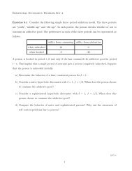
However, super-replication requires a rather low K 1 and hence a pretty high hedging
cost which amounts to even almost 7 times the basket option price for the case T = 1
and K = 1.10. Especially, Figure 1 is designed to demonstrate how K 1 influences the
hedging cost and the hedging error. Clearly, K 1 has two opposite effects on the hedging
18

Table 5: MC Simulated Basket Call Prices and Standard Errors (in Bracket)
for 100 Contracts with 500, 000 Simulations
T = 1 T = 3 T = 5 T = 10
K = 1.10 1.50 7.61 13.75 26.25
(0.0053) (0.0177) (0.0293) (0.0604)
K = 1.05 3.19 10.24 16.47 28.73
(0.0077) (0.0197) ( 0.0310) (0.0611)
K = 1.00 5.90 13.33 19.50 31.14
(0.0099) (0.0215) (0.0323) (0.0618)
K = 0.95 9.56 16.81 22.74 33.68
(0.0115) (0.0227) (0.0333) (0.0623)
K = 0.90 13.88 20.60 26.17 36.24
(0.0124) (0.0236) (0.0339) (0.0626)
Table 6: Super-Hedging Portfolio with Four Dominant Assets
K T BC 0 K 1 HC E[HE] k 2 k 3 k 6 k 7
1 13.88 0.46 30.30 -17.51 0.65/0.70 0.45/0.60 0.60/0.65 0.60/0.65
0.90
3 20.60 0.22 53.75 -40.01 0.30/0.45 0.15/0.30 0.30/0.45 0.30
5 26.17 0.08 63.52 -51.18 0/0.15 0/0.15 0/0.15 0/0.15
0.95
1.00
1.05
1.10
1 9.56 0.53 23.71 -15.08 0.75 0.60/0.65 0.70/0.75 0.70/0.75
3 16.81 0.24 51.89 -42.34 0.30/0.45 0.15/0.30 0.30/0.45 0.30/0.45
5 22.74 0.13 59.76 -50.70 0.15/0.30 0/0.15 0.15/0.30 0.15/0.30
1 5.90 0.56 21.78 -16.91 0.75/0.80 0.65/0.70 0.75/0.80 0.75
3 13.33 0.26 50.13 -44.46 0.30/0.45 0.15/0.30 0.30/0.45 0.30/0.45
5 19.50 0.15 58.84 -53.91 0.15/0.30 0/0.15 0.15/0.30 0.15/0.30
1 3.19 0.64 14.49 -12.04 0.85/0.90 0.75/0.80 0.85/0.90 0.85/0.90
3 10.24 0.38 40.17 -36.17 0.45/0.60 0.30/0.45 0.45/0.60 0.45/0.60
5 16.47 0.18 56.58 -54.96 0.15/0.30 0/0.15 0.15/0.30 0.15/0.30
1 1.50 0.70 10.01 -9.06 0.95 0.85/0.90 0.90/0.95 0.90/0.95
3 7.61 0.46 33.42 -31.17 0.65/0.70 0.45/0.60 0.65 0.60/0.65
5 13.75 0.19 55.78 -57.64 0.30 0.15 0.15/0.30 0.15/0.30
19

performance: a reduction in K 1 decreases the expected shortfall and meanwhile increases
the hedging cost. Thus, a higher hedging cost is unavoidable to achieve super-replication.
Besides, it demonstrates that the hedging strategy proposed in this paper is exactly to
achieve a trade-off between successful hedges and reduced hedging costs by varying strikes.
0.2
Expected Shortfall and Relative Hedging Cost vs. K 1
4
expected shortfall
0.15
0.1
0.05
0
0 0.1 0.2 0.3 0.4 0.5 0.6 0.7 0.8 0.9
K 1
0 0.1 0.2 0.3 0.4 0.5 0.6 0.7 0.8 0.9 0 1
3
2
relative hedging cost: HC 0
/BC 0
Figure 1: Expected Shortfall and Relative Hedging Cost vs. K 1 for
the Basket Call with T = 3 and K = 0.9
When relaxing the strong requirement of super-replication, the hedging cost can be
surely decreased, for instance, in the hedging portfolio obtained by taking the second
criterion. As formulated in the model, the variance of the hedging error is minimized
given a certain hedging cost V 0 . Here, two constraints are imposed on the hedging cost:
BC 0 , the basket option price, and HP (7), the hedging cost of the static super-hedging
portfolio with all 7 underlying assets. First as shown in Table 7, both constraints lead to
sub-replication, leaving some risks uncovered. Even for the case of T = 1 and K = 1.10,
there is no such a portfolio when V 0 = BC 0 due to the limited number of strikes traded
in the market. Given the strike set, all possible combinations of traded options have
higher prices than the basket call. As the ES (the identifier of the hedging performance)
decreases with the hedging cost, better results are achieved with the constraint of HP (7):
Opposite to the positive expected hedging error and high ES obtained in the case of
V 0 = BC, the hedging error turns out to be negative on average and the ES decreases
greatly to 4% − 9% across all maturities and strikes of the basket call. This result
indicates that hedging with four assets gives a relatively satisfactory performance: only a
reasonable low hedging error arises when investing the same capital as the hedging cost
of the super-hedging portfolio composed of plain-vanilla options on all 7 assets which
is supposed to be not available or at least not easily implementable. Moreover, such a
hedging portfolio creates far less transaction costs than the super-hedging portfolio based
on all the underlying assets if it exists. It enhances in turn the performance of the new
hedging strategy by using only 4 underlying assets.
In addition, one can easily observe that the hedging portfolio given V 0 = HP (7)
performs better for short maturity. The relative ES and the variance of the hedging error
of such portfolios always increase with T . Nevertheless, the variance of the hedging error
20

Table 7: Minimum-Variance Hedging Portfolio with Four Dominant Assets
K T BC0
0.90
0.95
1.00
1.05
1.10
V0 = BC0
V0 = HP (7)
HC E[HE] Var[HE] ES%
HP (7)
k2 k3 k6 k7 HC E[HE] Var[HE] ES% k2 k3 k6 k7
1 13.88 13.62 0.28 0.0008 9.48 0.85 0.80 0.95 0.85 15.05 14.93 -1.12 0.0007 4.80 0.85 0.70 0.95 0.85
3 20.60 20.57 0.03 0.0030 10.49 0.85 0.70 1.10 0.75 22.72 22.70 -2.54 0.0026 5.18 0.80 0.65 1.00 0.75
5 26.17 26.08 0.13 0.0054 11.25 0.80 0.60 1.10 0.75 28.43 28.41 -3.07 0.0051 6.22 0.75 0.60 1.00 0.70
10 36.24 36.10 0.26 0.0148 13.31 0.70 0.45 1.15 0.60 38.1 38.02 -3.36 0.0146 9.30 0.65 0.30 1.10 0.60
1 9.56 9.29 0.29 0.0010 14.89 0.95 0.85 1.10 0.90 11.50 11.36 -1.91 0.0008 4.56 0.90 0.80 1.00 0.90
3 16.81 16.76 0.05 0.0031 13.39 0.90 0.80 1.15 0.85 19.66 19.63 -3.41 0.0026 5.01 0.85 0.70 1.10 0.80
5 22.74 22.61 0.18 0.0058 13.49 0.90 0.65 1.15 0.85 25.68 25.58 -3.90 0.0051 6.13 0.85 0.60 1.10 0.75
10 33.68 33.64 0.07 0.0153 14.24 0.90 0.45 1.20 0.65 35.99 35.85 -4.08 0.0146 9.31 0.65 0.45 1.15 0.65
1 5.90 5.85 0.06 0.0010 21.03 1.00 0.95 1.15 1.00 8.48 8.26 -2.51 0.0007 4.45 0.95 0.90 1.05 0.95
3 13.33 12.97 0.45 0.0034 18.91 1.00 0.90 1.20 0.95 16.87 16.79 -4.17 0.0025 4.90 0.95 0.75 1.15 0.85
5 19.50 19.42 0.11 0.0061 15.97 0.95 0.75 1.20 0.95 23.11 23.07 -4.89 0.0050 5.76 0.85 0.65 1.15 0.85
10 31.14 31.11 0.06 0.0158 15.62 0.85 0.60 1.20 0.80 33.95 33.73 -4.86 0.0146 9.31 0.80 0.45 1.20 0.70
1 3.19 3.14 0.06 0.0008 31.82 1.05 1.10 1.20 1.10 6.04 5.74 -2.71 0.0006 4.30 1.00 1.00 1.10 1.00
3 10.24 10.11 0.16 0.0035 22.91 1.10 1.00 1.20 1.05 14.36 14.31 -4.92 0.0025 4.48 0.95 0.80 1.20 0.95
5 16.47 16.42 0.06 0.0066 19.32 1.10 0.90 1.20 1.00 20.73 20.55 -5.60 0.0050 5.74 0.95 0.70 1.20 0.90
10 28.73 28.67 0.12 0.0166 17.47 1.00 0.65 1.20 0.90 32.01 31.99 -6.11 0.0148 8.90 0.90 0.60 1.20 0.70
1 1.50 Given the strike set, all possible portfolios’ price is above BC0. 4.16 2.63 -1.20 0.0005 16.52 1.10 1.15 1.20 1.10
3 7.61 7.60 0.02 0.0037 29.07 1.20 1.15 1.20 1.15 12.14 11.88 -5.15 0.0024 4.57 1.05 0.90 1.20 1.00
5 13.75 13.70 0.08 0.0073 23.92 1.20 1.05 1.20 1.10 18.53 18.53 -6.55 0.0049 5.29 1.05 0.85 1.20 0.90
10 26.25 26.01 0.45 0.0180 20.46 1.10 0.80 1.20 1.00 30.15 30.05 -7.14 0.0148 8.72 0.95 0.65 1.20 0.80
Note: ES% denotes the relative ES, namely the expected value measured in percentage of shortfalls divided by the corresponding basket option payoffs at
the maturity date T .
21

and ES differ insignificantly across the strikes of the basket option. Unfortunately, such
general rules can not be summarized in the case of V 0 = BC. Especially, the hedging
performance surprisingly turns out to be poorest for the shortest maturity T = 1. As to
the obtained optimal strikes of the hedging portfolio, they generally increase with the
strike of the basket option in both cases. However, because S 6 is negatively correlated to
the other three assets, k 6 rises with T opposed to the decreasing relation of k 2 , k 3 , and
k 7 to the maturity.
The minimum-expected-shortfall hedging portfolios are demonstrated in Table
8 given the same two constraints on the hedging cost, BC 0 and HP (7). With a
restricted number of options, the obtained hedging portfolio sometimes coincides
with the minimum-variance hedging portfolio. Nevertheless, the risk measure in this
case is the expected shortfall, which is in effect a stricter criterion than the second
one concerning only the positive difference between the prices of the basket option
and the corresponding hedging portfolio. As a result, the hedging cost is generally
higher than that of the minimum-variance hedging portfolio. Obviously, it leads to a
better performance with lower hedging error and ES. To achieve a even smaller ES,
the hedging cost constraint is further raised in Table 9 to the Value at Risk at the
level 10% of the basket option discounted payoff. Due to the lack of the distribution
of the underlying basket, this has to be obtained by running simulations. Under
this construction, the hedging cost of the hedging portfolio becomes surely higher
(about V aR 0.10 ). It then gives a quite promising result that the ES is greatly reduced
and turns out to be almost zero, except those basket options with a long time to maturity.
As also observed in the results above, relatively lower hedging costs are required for
in- and at-the-money basket options to achieve almost the same relative ES compared
with out-of-the-money options. Consequently, if aiming at capturing the trade-off
between reduced hedging costs and successful replications, the hedging portfolio performs
better for in- and at-the-money basket options. To clearly show the regions of sub- and
super-replication, the payoffs of the basket option (T = 3, K = 0.9) and its minimum-ES
hedging portfolio given HC 0 = HP (7) are simulated and plotted in Figure 2. It can be
observed that the basket option is completely hedged if the realized value of the basket
is below or around the strike. The possibility of sub-replication rises with the value of
the basket being above 1.00. Nevertheless, the hedging error is rather small compared to
the basket option.
5.3 Remarks
Sometimes, the hedging performance is not that satisfactory especially for out-of-themoney
options. It is mainly due to the following two factors.
• First, the sub-hedge-basket is composed of simply dominant assets without reallocating
weights. Therefore, the value of the subset is only part of the original basket.
The only tool in the model to match the payoff of the basket option is varying the
strikes of the hedging instruments. However, their power to match the distribution
is fairly limited since they do not change the shape of the distribution of the
22

Table 8: Minimum-Expected-Shortfall Hedging Portfolios with Four Dominant Assets (I)
K T BC0
0.90
0.95
1.00
1.05
1.10
V0 = BC0
V0 = HP (7)
HC E[HE] Var[HE] ES%
HP (7)
k2 k3 k6 k7 HC E[HE] Var[HE] ES% k2 k3 k6 k7
1 13.88 13.82 0.07 0.0009 8.98 0.95 0.75 0.90 0.85 15.05 15.04 -1.23 0.0008 4.59 0.90 0.70 0.90 0.85
3 20.60 20.57 0.03 0.0030 10.49 0.85 0.70 1.10 0.75 22.72 22.70 -2.54 0.0011 5.18 0.80 0.65 1.00 0.75
5 26.17 26.17 0.01 0.0055 11.14 0.70 0.65 1.15 0.75 28.43 28.41 -3.07 0.0051 6.22 0.75 0.60 1.00 0.70
10 36.24 36.24 -0.01 0.0149 12.98 0.65 0.45 1.10 0.65 38.10 38.10 -3.50 0.0147 9.20 0.75 0.30 1.00 0.60
1 9.56 9.55 0.01 0.0011 13.60 0.90 0.85 1.15 0.90 11.50 11.48 -2.04 0.0009 4.39 0.90 0.75 1.05 0.90
3 16.81 16.78 0.04 0.0032 13.35 0.95 0.75 1.15 0.85 19.66 19.63 -3.41 0.0026 5.01 0.85 0.70 1.10 0.80
5 22.74 22.69 0.08 0.0059 13.32 0.90 0.60 1.20 0.85 25.68 25.64 -3.97 0.0052 6.07 0.75 0.65 1.15 0.75
10 33.68 33.68 -0.02 0.0155 14.19 0.85 0.60 1.10 0.65 35.99 35.95 -4.26 0.0148 9.19 0.80 0.45 1.00 0.65
1 5.90 5.85 0.06 0.0010 21.03 1.00 0.95 1.15 1.00 8.48 8.40 -2.66 0.0008 4.14 0.95 0.85 1.10 0.95
3 13.33 13.31 0.03 0.0035 17.46 1.05 0.95 1.15 0.90 16.87 16.85 -4.24 0.0026 4.78 0.90 0.80 1.05 0.90
5 19.50 19.46 0.06 0.0062 15.90 1.00 0.70 1.20 0.95 23.11 23.10 -4.92 0.0050 5.75 0.90 0.60 1.15 0.85
10 31.14 31.14 -0.01 0.0159 15.58 0.85 0.65 1.15 0.80 33.95 33.94 -5.26 0.0149 9.02 0.85 0.45 1.05 0.75
1 3.19 3.14 0.06 0.0008 31.82 1.05 1.10 1.20 1.10 6.04 6.01 -3.00 0.0007 3.68 1.00 0.90 1.10 1.05
3 10.24 10.17 0.09 0.0036 22.67 1.15 0.95 1.20 1.05 14.36 14.31 -4.92 0.0025 4.48 0.95 0.80 1.20 0.95
5 16.47 16.42 0.06 0.0066 19.32 1.10 0.90 1.20 1.00 20.73 20.71 -5.81 0.0051 5.55 0.90 0.70 1.15 0.95
10 28.73 28.73 -0.06 0.0169 17.36 1.10 0.60 1.15 0.90 32.01 32.01 -6.21 0.0149 8.89 0.80 0.70 1.20 0.70
1 1.50 Given the strike set, all possible portfolios’ price is above BC0. 4.16 4.11 -2.77 0.0006 2.68 1.05 1.05 1.15 1.05
3 7.61 7.60 0.02 0.0037 29.07 1.20 1.15 1.20 1.15 12.14 12.14 -5.47 0.0025 4.22 1.05 0.80 1.20 1.05
5 13.75 13.78 -0.03 0.0074 23.73 1.10 1.15 1.20 1.10 18.53 18.53 -6.55 0.0049 5.29 1.05 0.85 1.20 0.90
10 26.25 26.21 -0.08 0.0181 19.85 1.20 0.85 1.20 0.90 30.15 30.12 -7.27 0.0151 8.70 1.05 0.60 1.15 0.80
23

K T BC 0
V 0 = V aR 10%
HC E[HE] Var[HE] ES% k 2 k 3 k 6 k 7
0.90
0.95
1.00
1.05
1.10
1 13.88 24.57 -11.38 0.0007 0.0009 0.45 0.65 0.95 0.70
3 20.60 38.13 -21.17 0.0023 0.0061 0.15 0.30 0.90 0.65
5 26.17 48.12 -30.07 0.0045 0.0141 0.15 0.45 0.85 0.15
10 36.24 60.15 -44.90 0.0143 0.1148 0 0.30 0 0.15
1 9.56 19.91 -11.02 0.0006 0.0012 0.75 0.65 0.90 0.75
3 16.81 34.19 -21.00 0.0021 0.0065 0.70 0.30 1.00 0.45
5 22.74 44.49 -29.81 0.0047 0.0200 0.30 0.30 1.20 0.15
10 33.68 58.95 -47.46 0.0140 0.0950 0.15 0.30 0 0.15
1 5.90 15.21 -9.92 0.0007 0.0039 0.90 0.75 1.00 0.75
3 13.33 30.29 -20.48 0.0021 0.0072 0.65 0.30 0.95 0.70
5 19.50 41.10 -29.59 0.0042 0.0164 0.65 0.30 1.15 0.15
10 31.14 58.54 -51.44 0.0136 0.0713 0.15 0.15 0.15 0.15
1 3.19 10.63 -7.92 0.0008 0.0111 0.80 0.85 1.05 0.95
3 10.24 26.28 -19.37 0.0023 0.0179 0.75 0.65 1.00 0.60
5 16.47 37.55 -28.88 0.0041 0.0195 0.15 0.30 1.05 0.70
10 28.73 56.58 -52.30 0.0134 0.0617 0.15 0.15 0.15 0.30
1 1.50 6.01 -4.80 0.0009 0.1631 1.00 0.90 1.10 1.05
3 7.61 22.27 -17.71 0.0027 0.0130 0.80 0.60 1.10 0.75
5 13.75 34.30 -28.16 0.0043 0.0207 0.45 0.30 1.05 0.70
10 26.25 53.75 -51.62 0.0130 0.0702 0.15 0.15 0.60 0.15
Table 9: Minimum-Expected-Shortfall Hedging Portfolios with Four Dominant Assets (II)
Figure 2: Simulations of the Basket Option (T=3, K=0.9) and the Minimum-Expected-
Shortfall Hedge Portfolio with Constraint V 0 = V aR 0.10
24

sub-hedge-basket, but only shift the distribution closer to the original basket. This
can be easily observed in Figure 3. By neglecting those insignificant underlying
assets, the sub-basket experiences less extreme cases. However, since it is part of
the original basket, it is located on the left of the original basket. Therefore, the
function of varying strikes is to relocate the distribution of the hedging portfolio to
the proper position near the basket option. As shown in the figure, the tighter the
hedging criterion is, the further the distribution is shifted to the right.
• In addition, all the hedging portfolios designed in this paper are static. Hence,
more capital may be required to well hedge the basket option. However, the model
is restricted to be static under the construction of hedging with plain-vanilla options
on the significant underlying assets. As the control variables in this model are strikes
of these options, frequent trading on options with different strikes would cause great
loss and additional transaction costs.
0.045
0.04
0.035
Distribution of the Basket Option and Hedging Portfolios
Basket Option
Super−hedge
Variance Hedge−BC
ES Hedge−HP7
ES Hedge−VaR0.10
0.03
Distribution
0.025
0.02
0.015
0.01
0.005
0
−0.5 0 0.5 1 1.5 2
7
4
(Σ j=1
ω j
S j
(T) − K) and Σ j=1
ω j
(S j
(T) − k j
)
Figure 3: Distribution of the Underlying Basket (T=3, K=0.9) and the Hedging Portfolios
As a result, other control variables have to be considered to improve the hedging effect.
One possible instrument is reallocating the weights of the hedging basket such that the
new sub-hedge-basket can better match the distribution of the original basket. On this
basis, dynamic hedging would also be possible by duplicating the basket option with the
hedging assets. This would be an extension to be considered in future works.
6 Conclusion
In summary, Principal Components Analysis, a popular multivariate statistical method
for dimension reduction, is applied to basket options hedging to select only a subset
of underlying assets. The selection procedure is completed mainly by decomposing the
modified covariance structure of the underlying basket into eigenvalues in the order of
significance and eigenvectors. Hedging basket options based on only several assets can not
only reduce transaction costs if combined with other hedging strategies, but also become
practical and essential when some of the underlying assets are illiquid or not even available
25

for trading. Following this idea, a new two-step static hedging strategy is developed in
this paper. It consists of plain-vanilla options on N 1 < N dominant assets with optimal
strike prices. The strikes are optimally chosen by numerically solving an optimization
problem where the optimality criterion depends on the risk attitude of hedgers. As given
in the paper, the first objective is to eliminate all the risks that the basket option is
exposed to. Alternatively, optimal strikes are obtained by minimizing a particular risk
measure, e.g., the variance of the hedging error or the expected shortfall, given a constraint
on the hedging cost. Meanwhile considering the limited number of strikes traded in
the market, complicated numerical optimizations have to be done by imposing another
constraint that the optimal strikes are in the set of traded assets. Particularly, a simple and
computationally efficient calibration procedure, convexity correction, is designed when
achieving the super-replication hedging portfolio. As observed from the numerical results,
the static hedging method achieves the trade-off between reduced hedging cost and overall
super-replication. It demonstrates also that hedging with only a subset of assets works
quite well even without considering reduced transaction costs, generating a reasonably
small hedging error by investing the same capital as the super-hedging portfolio on all
the underlying assets which is difficult to construct or is even not available in the market.
Actually, its performance will become more satisfactory if the underlying basket is large
and illiquid. Since the hedging performance is sensitive to the subset of the selected assets,
it is recommended to examine hedging costs, involved transaction costs as well as hedging
errors of several subsets. To achieve a better performance, hedging basket options with
a subset of assets could be improved by reallocating weights of the sub-hedge-basket to
approximately match the distribution of the original basket. This could be the extension
for future research.
26

References
[1] Ashraff, J., J. Tarczon and W.Q. Wu (1995) Safe Crossing, RISK, 8 (7), pp. 56 − 57.
[2] D’Aspremont, A. and L. El-Ghaoui (2003) Static Arbitrage Bounds on Basket Options,
to appear in Mathematical Programming, Series A.
[3] Beisser, J. (2001) Tropics in Finance - A Conditional Expectation Approach to Value
Asian, Basket and Spread Options, PhD thesis, Johannes-Gutenberg-Universität
Mainz.
[4] Black, F. and M. Scholes, (1973) The Pricing of Options and Corporate Liabilities,
Journal of Political Economy, Vol. 81, pp. 637 − 654.
[5] Cherubini, U. and E. Luciano (2002) Bivariate Option Pricing with Copulas, Applied
Mathematical Finance, 9 (2), pp. 69 − 86.
[6] Curran, M. (1994) Valuing Asian and Portfolio Options by Conditioning on the
Geometric Mean Price, Management Science, 40, pp. 1705 − 1711.
[7] Dahl, L.O. and F. E. Benth (2002) Valuation of Asian Basket Options with Quasi-
Monte Carlo Techniques and Singular Value Decomposition, Monte Carlo and Quasi-
Monte Carlo Methods 2000, K,-T. Fang, F.J. Hickernell and H. Niederreiter (eds.),
Springer Verlag, pp. 201 − 214.
[8] Deelstra, G., J. Liinev, and M. Vanmaele (2004) Pricing of Arithmetic Basket Options
by Conditioning, Insurance: Mathematics and Economics, 34 (1), pp. 1 − 23.
[9] Engelmann, B. and P. Schwendner (2001) Effizientes Pricing und Hedging von Multi-
Asset Opionen, Beitrag zum Handbuch Gesamtbanksteuerung, Hrsg. R. Eller, W.
Gruber, M. Reif, Schäffer-Poeschel Verlag.
[10] Fengler, M., W. Härdle and P. Schmidt (2002) The Analysis of Implied Volatilities,
Applied Quantitative Finance, Springer, pp. 127 − 144.
[11] Harman, H. H. (1967) Mordern Factor Analysis, the University of Chicago Press,
Chicago and Landon.
[12] Härdle, W. and L. Simar (2003) Applied Multivariate Statistical Analysis, Springer.
[13] Haug, Espen Gaarder (1997) The Complete Guide to Option Pricing Formulas,
McGraw-Hill.
[14] Hobson, D., P. Laurence and T. Wang (2005) Static Arbitrage Upper Bounds for
Basket Options, Quantitativ Finance, Vol. 5, No. 4, August 2005, pp. 329 − 342.
[15] Hotelling, H. (1933) Analysis of a Complex of Statistical Variables into Principal
Components, Journal of Educational Psychology, 24, pp. 498-520.
[16] Joe, H. (1997) Multivariate Models and Dependence Concepts, Chapman and Hall,
London.

[17] Lamberton, D. and B. Lapeyre (1992) Hedging Index Options with Few Assets,
Mathematical Finance, Vol. 3, No. 1, pp. 25 − 41.
[18] Laurence, P. and T.H. Wang, (2003) Sharp Upper and Lower Bounds for Basket
Options, to appear in Quantitative Finance.
[19] Milevsky, M. A. and S. E. Posner (1998) A Closed-Form Approximation for Valuing
Basket Options, The Journal of Derivatives, Vol. 5(4), Summer 1998, pp. 54 − 61.
[20] Nelken, Israel (1999) Pricing, Hedging & Trading Exotic Options: Understand the
Intricacies of Exotic Options and How to Use Them to Maximum Advantage, Irwin.
[21] Nielsen, J.A. and K. Sandmann (2003) Pricing Bounds on Asian Options, Journal of
Financial and Quantitive Analysis, 38, No. 2.
[22] Pearson, K. (1901) On Lines and Planes of Closest Fit to Systems of Points in Space,
Philosophical Magazine, Ser. 6, 2, pp. 559 − 572.
[23] Pellizzari, P. (1998) Efficient Monte Carlo Pricing of Basket Options, Economics
Working Paper Archive (EconWPA).
[24] Pellizzari, P. (2004) Static Hedging of Multivariate Derivatives by Simulation, forthcoming
in European Journal of Operations Research.
[25] Rogers, L.C.G. and Z. Shi (1995) The Value of an Asian Option, Journal of Applied
Probability, 32, pp. 1077 − 1088.
[26] Simon, S., M.J. Goovaerts and J. Dhaene (2000) An Easy Computable Upper Bound
for the Price of an Arithmetic Asian Option, Insurance: Mathematics and Economics,
vol. 26, issue 2-3, pp. 175 − 183.
[27] Srirastava, M.S. and C. G. Khatri (1979) An Introduction to Multivariate Statistics,
Elsevier North Holland Inc..

Appendix: Proof of Proposition 1
Proof. First, the Lagrange function for the minimization problem is formed
N∑
L = ω i e −rT E [ (
(S i (T ) − k i ) +] N
)
∑
+ λ ω i k i − K
=
i=1
N∑
∫ ∞
ω i e −rT
i=1
max(k i ,0)
i=1
( N
)
∑
(x i − k i ) f i (x i )dx i + λ ω i k i − K
where f i (x i ) is the lognormal density function under the risk-neutral martingale measure
for the stock S i . A necessary and sufficient condition for the sequence k i to minimize the
Lagrange function is found through the first order conditions:
∂L
= −ω i e −rT ∂max (k i, 0)
{max (k i , 0) − k i } f i [max (k i , 0)]
∂k i ∂k
∫ i
∞
−ω i e −rT f i (x i )dx i + λω i
max(k i ,0)
= 0
N
∂L
∂λ = ∑
ω i k i − K = 0.
i=1
These conditions can be further simplified to
( ∫
∂L
∞
)
= −ω i e −rT f i (x i )dx i − λ = 0
∂k i
∀ i = 1, · · · , N (16)
max(k i ,0)
N
∂L
∂λ = ∑
ω i k i − K = 0 (17)
i=1
since the term of the first condition ω i e −rT ∂max(k i ,0)
∂k i
{max (k i , 0) − k i } f i [max (k i , 0)] is
always equal to zero no matter which value max (k i , 0) is going to take.
With these conditions, one can first prove that k i ∈ [0, K] ∀ i = 1, · · · , N is always
satisfied. Assume any specific i we have k i < 0. This implies that
∂L
∂k i
| ki =k i
= −ω i
(
e −rT − λ ) = 0.
In this case, the first order condition (16) can be reduced to
∫ ∞
max(k i ,0)
i=1
f i (x i )dx i = 1 ∀ i = 1, · · · , N,
which implies the result that k i ≤ 0 ∀ i = 1, · · · , N. This contradicts however the
second first order condition (17). Therefore, k i ’s are always positive and lie in the interval
[0, K].

Then, given k i ∈ [0, K], ∀ i = 1, · · · , N, the first order condition (16) can be stated as
Φ(d 2 (S i , k i )) = Φ(d 2 (S j , k j )) ∀ i, j
where d 2 (S i , k i ) = ln Si (0)
+(r−q k i − 1
i 2 σ2 i
√ )T
σ i T
as defined in the BS formula, and Φ again denotes
the standard normal cumulative distribution function.
Furthermore, Φ(x) is bijective, the first condition (16) can be reduced to
Then k i can be all expressed in k 1 as
( ) {
σ i
k1 σ 1
k i = S i exp T
S 1
d 2 (S i , k i ) = d 2 (S j , k j ) ∀ i = 1, · · · , N.
[ (
1 − σ i
σ 1
) (
r + 1 2 σ 1σ i
)
+
(
σi
σ 1
q 1 − q i
) ]} (18)
In summary, the optimal k i ’s are all positive and determined by solving the system of
equations
( ) { [ σ i
k1 σ
(
1
k i = S i exp T 1 − σ ) (
i
r + 1 ) ( ) ]}
S 1 σ 1 2 σ σi
1σ i + q 1 − q i
σ 1
N∑
ω i k i = K.
i=1
The existing problem is whether there is always a solution and whether the solution
is unique. This is shown in the following way:
First, k i is a strictly increasing function of k 1 since the first derivative of k i with respect
to k 1
k i ′ = S ( ) { [
iσ σ i −1
i k1 σ
(
1
exp T 1 − σ ) (
i
r + 1 ) ( ) ]}
S 1 σ 1 S 1 σ 1 2 σ σi
1σ i + q 1 − q i
σ 1
is always larger than zero.
Then the sum of the k i ’s as a function of k 1 given by
N∑ N∑
( ) {
σ i
k1 σ 1
g(k 1 ) = k i = S i exp T
S 1
i=1
i=1
[ (
1 − σ i
σ 1
) (
r + 1 2 σ 1σ i
)
+
(
σi
σ 1
q 1 − q i
) ]}
is also continuous and increasing in k 1 , which could be proven again by checking its first
derivative. Moreover,
g(k 1 = 0) = 0,
and
g(k 1 = K) =
n∑
1=1
( ) { [
K σ i
σ
(
1
S i exp T 1 − σ i
S 1
= K + S 2
( K
S 1
) σ 2
σ 1
exp
{
≥ K.
T
σ 1
) (
r + 1 2 σ 1σ i
)
+
[ (
1 − σ 2
σ 1
) (
r + 1 2 σ 1σ 2
)
+
As a consequence, there is always a unique solution k i ∈ [0, K].
(
σi
) ]}
q 1 − q i
σ 1
( ) ]}
σ2
q 1 − q 2 + · · ·
σ 1