Automatic Non-Rigid 3D Modeling from Video - University of Toronto ...

Automatic Non-Rigid 3D Modeling from Video
Lorenzo Torresani 1 and Aaron Hertzmann 2
1 Stanford University, Stanford, CA, USA
ltorresa@cs.stanford.edu
2 University of Toronto, Toronto, ON, Canada
hertzman@dgp.toronto.edu
Abstract. We present a robust framework for estimating non-rigid 3D
shape and motion in video sequences. Given an input video sequence, and
a user-specified region to reconstruct, the algorithm automatically solves
for the 3D time-varying shape and motion of the object, and estimates
which pixels are outliers, while learning all system parameters, including
a PDF over non-rigid deformations. There are no user-tuned parameters
(other than initialization); all parameters are learned by maximizing the
likelihood of the entire image stream. We apply our method to both rigid
and non-rigid shape reconstruction, and demonstrate it in challenging
cases of occlusion and variable illumination.
1 Introduction
Reconstruction from video promises to produce high-quality 3D models for many
applications, such as video analysis and computer animation. Recenly, several
“direct” methods for shape reconstruction from video sequences have been demonstrated
[1–3] that can give good 3D reconstructions of non-rigid 3D shape, even
from single-view video. Such methods estimate shape by direct optimization
with respect to raw image data, thus avoiding the difficult problem of tracking
features in advance of reconstruction. However, many difficulties remain for developing
general-purpose video-based reconstruction algorithms. First, existing
algorithms make the restrictive assumption of color constancy, that object features
appear the same in all views. Almost all sequences of interest violate this
assumption at times, such as with occlusions, lighting changes, motion blur, and
many other common effects. Second, non-rigid shape reconstruction requires a
number of regularization parameters (or, equivalently, prior distributions), due
to fundamental ambiguities in non-rigid reconstruction [4, 5], and to handle noise
and prevent over-fitting. Such weights must either be tuned by hand (which is
difficult and inaccurate, especially for models with many parameters) or learned
from annotated training data (which is often unavailable, or inappropriate to
the target data).
In this paper, we describe an algorithm for robust non-rigid shape reconstruction
from uncalibrated video. Our general approach is to pose shape reconstruction
as a maximum likelihood estimation problem, to be optimized with
respect to the entire input video sequence. We solve for 3D time-varying shape,

2 L. Torresani and A. Hertzmann
correspondence, and outlier pixels, while simultaneously solving for all weighting/PDF
parameters. By doing so, we exploit the general property of Bayesian
learning that all parameters may be estimated by maximizing the posterior distribution
for a suitable model. No prior training data or parameter tuning is
required. This general methodology — of simultaneously solving for shape while
learning all weights/PDF parameters — has not been applied to 3D shape reconstruction
from video, and has only rarely been exploited in computer vision
in general (one example is [6]).
This paper begins with a general framework for robust shape reconstruction
from video. This model is based on robust statistics: all violations of color
constancy are modeled as outliers. Unlike robust tracking algorithms, we solve
for shape globally over an entire sequence, allowing us to handle cases where
many features are completely occluded in some frames. (A disadvantage of our
approach is that it cannot currently be applied to one-frame-at-a-time tracking).
We demonstrate sequences for which previous global reconstruction methods fail.
For example, previous direct methods require that all feature points be visible
in all video frames, i.e. all features are visible in a single “reference frame;” our
method relaxes this assumption and allows sequences for which no single “reference
frame” exists. We also show examples where existing techniques fail due to
local changes in lighting and shape. Our method is based on the EM algorithm
for robust outlier detection. Additionally, we show how to simultaneously solve
for the outlier probabilities for the target sequence.
We demonstrate the reconstruction framework in the case of rigid motion
under weak perspective projection, and non-rigid shape under orthographic projection.
In the latter case, we do not assume that the non-rigid geometry is
known in advance. Separating non-rigid deformation from rigid motion is ambiguous
without some assumptions about deformation [4, 5]. Rather than specify
the parameters of a shape prior in advance, our algorithm learns a shape PDF
simultaneously with estimating correspondence, 3D shape reconstruction, and
outliers.
1.1 Relation to Previous Work
We build on recent techniques for exploiting rank constraints on optical flow in
uncalibrated single-view video. Conventional optical flow algorithms use only local
information; namely, every track in every frame is estimated separately [7, 8].
In contrast, so-called “direct methods” optimize directly with respect to the raw
image sequence [9]. Irani [1] treated optical flow in rigid 3D scenes as a global
problem, combining information from the entire sequence — along with rank
constraints on motion — to yield better tracking. Bregler et al. [10] describe an
algorithm for solving for non-rigid 3D shape from known point tracks. Extending
these ideas, Torresani et al. [2, 11] and Brand [3] describe tracking and reconstruction
algorithms that solve for 3D shape and motion from sequences, even
for non-rigid scenes. Note that adding robustness to the above methods is nontrivial,
since this would require defining a unified objective function for tracking
and reconstruction that is not present in the previous work. Furthermore, one

Automatic Non-Rigid 3D Modeling from Video 3
must introduce a large number of hand-tuned weighting and regularization constraints,
especially for non-rigid motion, for which reconstruction is ill-posed
without some form of regularization [4, 5]. In our paper, we show how to cast
the problem of estimating 3D shape and motion from video sequences as optimization
of a well-defined likelihood function. This framework allows several
extensions: our method automatically detects outliers, and all regularization parameters
are automatically learned via Bayesian learning. Our non-rigid model
incorporates our previous work on non-rigid structure-from-motion [5], in which
reliable tracking data was assumed to be available in advance.
A common approach to acquiring rigid shape from video is to separate feature
selection, outlier rejection, and shape reconstruction into a series of stages,
each of which has a separate optimization process (e.g. [12]). Dellaert et al. [13]
solve for rigid shape while detecting outliers, assuming that good features can
be located in advance. The above methods assume that good features can be detected
in each frame by a feature detector, and that noise/outlier parameters are
known in advance. In contrast to these methods, we optimize the reconstruction
directly with respect to the video sequence.
Robust algorithms for tracking have been widely explored in local tracking
(e.g. [14–16]). Unlike local robust methods, our method can handle features that
are completely occluded, by making use of global constraints on motion. Similar
to Jepson et al. [16], we also learn the parameters at the same time as tracking,
rather than assuming that they are known a priori. Our outlier model is closely
related to layer-based motion segmentation algorithms [6, 17, 18], which are also
often applied globally to a sequence. We use the outlier model to handle general
violations of color constancy, rather than to specifically model multiple layers.
2 Robust Shape Reconstruction Framework
We now describe our general framework for robust shape reconstruction from
uncalibrated video. We then specialize this framework to rigid 3D motion in
Section 3, and to non-rigid motion in Section 4.
2.1 Motion model
We assume that 3D shape can be described in terms of the 3D coordinates
s j,t = [X j,t , Y j,t , Z j,t ] T of J scene points, over T time steps. The parameter
j indexes over points in the model, and t over time. We collect these points
in a matrix S t = [s 1,t , ..., s J,t ]. We parameterize 3D shape with a function as
S t = Γ (z t ; ψ), where z t is a hidden random variable describing the shape at
each time t, with a prior p(z t ); ψ are shape model parameters. The details of
these functions depend on the application. For example, in the case of rigid shape
(Section 3), we use Γ (z t ; ψ) = ¯S, i.e. the shape stays fixed at a constant value ¯S,
and ψ = {¯S}. For non-rigid shape (Section 4), Γ (z t ; ψ) is a linear combination
of basis shapes, determined by the time-varying weights z t ; ψ contains the shape
basis.

4 L. Torresani and A. Hertzmann
Additionally, we define a camera model Π. At a given time t, point j projects
to a 2D position p j,t = [x j,t , y j,t ] T = Π(s j,t ; ξ t ), where ξ t are the time-varying
parameters of the camera model. For example, ξ t might define the position and
orientation of the camera with respect to the object.
In cases when the object is undergoing rigid motion, we subsume it in the
rigid motion of the camera. This applies in both the case of rigid shape and nonrigid
shape. In the non-rigid case, we can generally think of the object’s motion
as consisting of a rigid component plus a non-rigid deformation. For example, a
person’s head can move rigidly (e.g. turning left or right) while deforming (due to
changing facial expressions). One might wish to separate rigid object motion from
rigid camera motion in other applications, such as under perspective projection.
2.2 Image model
We now introduce a generative model for video sequences, given the motion
of the 2D point tracks p j,t . Individual images in a video sequence are created
from the 2D points. Ideally, the window of pixels around each point p j,t should
remain constant over time; however, this window may be corrupted by noise and
outliers. Let w be an index over a pixel window, so that I w (p j,t ) is the intensity
of a pixel in the window 1 of point j in frame t. This pixel intensity should ideally
be a constant Īw,j; however, it will be corrupted by Gaussian noise with variance
σ 2 . Moreover, it may be replaced by an outlier, with probability 1−τ. We define
a hidden variable W w,j,t so that W w,j,t = 0 if the pixel is replaced by an outlier,
and W w,j,t = 1 if it is valid. The complete PDF over individual pixels in a
window is given by:
p(W w,j,t = 1) = τ (1)
p(I w (p j,t )|W w,j,t = 1, p j,t , Īw,j, σ 2 ) = N (I w (p j,t )|Īw,j; σ 2 ) (2)
p(I w (p j,t )|W w,j,t = 0, p j,t , Īw,j, σ 2 ) = c (3)
where N (I w (p j,t )|Īw,j; σ 2 ) denotes a 1D Gaussian distribution with mean Īw,j
and variance σ 2 , and c is a constant corresponding to the uniform distribution
over the range of valid pixel intensities. The values Īw,j are determined by the
corresponding pixel in the reference frame.
For convenience, we do not model the appearance of video pixels that do not
appear near 2D points, or correlations between pixels when windows overlap.
2.3 Problem statement
Given a video sequence I and 2D point positions specified in some reference
frames, we would like to estimate the positions of the points in all other frames,
and, additionally, learn the 3D shape and associated parameters.
1 In other words, I w(p j,t) = I (t) (p j,t + d w) where I (t) is the image at time t, and d w
represents the offset of point w inside the window.

Automatic Non-Rigid 3D Modeling from Video 5
We propose to solve this estimation problem by maximizing the likelihood of
the image sequence given the model. We encapsulate the parameters for the image,
shape, and camera model into the parameter vector θ = {Ī, σ2 , τ, ψ, ξ 1 , ..., ξ T }.
The likelihood itself marginalizes over the hidden variables W w,j,t and z t . Consequently,
our goal is to solve for θ to maximize
p(I|θ) = ∏ p(I w (p j,t )|θ) = ∏ ∫
∑
p(I, z t , W w,j,t |θ)dz t (4)
w,j,t
w,j,t z t
W w,j,t∈{0,1}
(We have replaced I w (p j,t ) with I for brevity). In other words, we wish to solve
for the camera motion, shape PDF, and outlier distribution from the video sequence
I, averaging over the unknown shapes and outliers.
2.4 Variational bound
In order to optimize Equation 4, we use an approach based on variational learning
[19]. Specifically, we introduce a distribution Q(W w,j,t , z t ) to approximate
the distribution over the hidden parameters at time t, and then apply Jensen’s
inequality to derive an upper bound on the negative log likelihood: 2
− ln p(I|θ) = − ln ∏ ∫
∑
p(I, z t , W w,j,t |θ)dz t (5)
w,j,t z t
= − ∑ ∫
ln
w,j,t
≤ − ∑ ∫
w,j,t z t
W w,j,t∈{0,1}
∑
z t W w,j,t∈{0,1}
∑
W w,j,t∈{0,1}
p(I, z t , W w,j,t |θ) Q(W w,j,t, z t )
Q(W w,j,t , z t ) dz t (6)
Q(W w,j,t , z t ) ln p(I, z t, W w,j,t |θ)
dz t (7)
Q(W w,j,t , z t )
We can minimize the negative log likelihood by minimizing Equation 7 with
respect to θ and Q. Unfortunately, even representing the optimal distribution
Q(W w,j,t , z t ) would be intractable, due to the large number of point tracks.
To make it manageable, we represent the distribution Q with a factored form:
Q(W w,j,t , z t ) = q(z t )q(W w,j,t ), where q(z t ) is a distribution over z t for each
frame, and q(W w,j,t ) is a distribution over whether each pixel (w, j, t) is valid
or an outlier. The distribution q(z t ) can be thought of as approximating to
p(z t |I, θ), and q(W w,j,t ) approximates the distribution p(W w,j,t |I, θ). Substituting
the factored form into Equation 7 gives the variational free energy (VFE)
F(θ, q):
F(θ, q) = − ∑ w,j,t
∫
∑
z t W w,j,t∈{0,1}
q(W w,j,t )q(z t ) ln p(I, z t, W w,j,t |θ)
q(W w,j,t )q(z t ) dz t (8)
In order to estimate shape and motion from video, our new goal is to minimize
F with respect to θ and q over all points j and frames t. For brevity, we write
2 We require that ∏ w,j,t
∫z t
∑W w,j,t ∈{0,1}
Q(Ww,j,t, zt) = 1, in order for Jensen’s
inequality to hold.

6 L. Torresani and A. Hertzmann
γ w,j,t ≡ q(W w,j,t = 1). Substituting the image model from Section 2.2 and
defining the expectation E q(zt)[f(z t )] ≡ ∫ q(z t )f(z t )dz t gives
F(θ, q, γ) = ∑ w,j,t
γ w,j,t E q(zt)[(I w (p t,j ) − Īw,j) 2 ]/(2σ 2 ) + ln √ 2πσ 2 ∑ w,j,t
γ w,j,t
−NJ ∑ t
E q(zt)[ln p(z t )] − ln c ∑ w,j,t
(1 − γ w,j,t ) − ln τ ∑ w,j,t
γ w,j,t
− ln(1 − τ) ∑ w,j,t
∑
(1 − γ w,j,t ) + NJ ∑ t
w,j,t(1 − γ w,j,t ) ln(1 − γ w,j,t ) + ∑ w,j,t
E q(zt)[ln q(z t )] +
γ w,j,t ln γ w,j,t + constants (9)
where N is the number of pixels in a window. Although there are many terms in
this expression, most terms have a simple interpretation. Specifically, we point
out that the first term is a weighted image matching term: for each pixel, it
measures the expected reconstruction error from comparing an image pixel to
its mean intensity Īw,j, weighted by the likelihood γ w,j,t that the pixel is valid.
2.5 Generalized EM algorithm
We optimize the VFE using a generalized EM algorithm. In the E-step we keep
the model parameters fixed and update our estimate of the hidden variable
distributions. The update rule for q(z t ) will depend on the particular motion
model specified by Γ . The distribution γ w,j,t (which indicates whether pixel
(w, j, t) is an outlier) is estimated as:
α 0 = p(I w (p j,t )|W w,j,t = 0, p j,t , θ)p(W w,j,t = 0|θ) = (1 − τ)c (10)
α 1 = p(I w (p j,t )|W w,j,t = 1, p j,t , θ)p(W w,j,t = 1|θ) (11)
τ
= √
2πσ
2 e−E q(z t )[(I w(p t,j)−Īw,j)2 ]/(2σ 2 )
(12)
Then, using Bayes’ Rule, we have the E-step for γ w,j,t :
γ w,j,t ← α 1 /(α 0 + α 1 ) (13)
In the generalized M-step, we solve for optical flow and 3D shape given the
outlier probabilities γ w,j,t . The outlier probabilities provide a weighting function
for tracking and reconstruction: pixels likely to be valid are given more weight.
Let p 0 j,t represent the current estimate of p j,t at a step during the optimization.
To solve for the motion parameters that define p j,t , we linearize the target image
around p 0 j,t : I w (p j,t ) ≈ I w (p 0 j,t) + ∇I T w (p j,t − p 0 j,t) (14)
where ∇I w denotes a 2D vector of image derivatives at I w (p 0 j,t ). One such linearization
is applied for every pixel w in every window j for every frame t at
every iteration of the algorithm.

Automatic Non-Rigid 3D Modeling from Video 7
Substituting Equation 14 into the first term of the VFE (Equation 9) yields
the following quadratic energy function for the motion: 3
∑
w,j,t
where
γ w,j,t
2σ 2 E q(z t)[(I w (p t,j ) − Īw,j) 2 ] ≈ ∑ j,t
E q(zt)[(p j,t − ˆp j,t ) T e j,t (p j,t − ˆp j,t )]
(15)
e j,t = 1 ∑
2σ 2 γ w,j,t ∇I w ∇Iw T (16)
w
ˆp j,t = p 0 j,t + 1
2σ 2 e−1 j,t
∑
γ w,j,t (Īw,j − I w (p 0 j,t))∇I w (17)
w
Hence, optimizing the shape and motion with respect to the image is equivalent
to solving the structure-from-motion problem of fitting the “virtual point tracks”
ˆp j,t , each of which has uncertainty specified by a 2×2 covariance matrix e −1
j,t . In
the next sections, we will outline the details of this optimization for both rigid
and non-rigid motion.
The noise variance and the outlier prior probability are also updated in the
M-step, by optimizing F(θ, q, γ) for τ and σ 2 :
τ ← ∑ w,j
σ 2 ← ∑ w,j,t
γ w,j,t /(JNT ) (18)
γ w,j,t E q(zt)[(I w (p j,t ) − Īw,j) 2 ]/ ∑ w,j
γ w,j,t (19)
The σ 2 update can be computed with Equation 15. These updates can be interpreted
as the expected percentage of outliers, and the expected image variance,
respectively.
3 Rigid 3D Shape Reconstruction from Video
The general-purpose framework presented in the previous section can be specialized
to a variety of projection and motion models. In this section we outline
the algorithm in the case of rigid motion under weak orthographic projection.
This projection model can be described in terms of parameters ξ t = {α t , R t , t t }
and projection function
Π(s j,t ; {α t , R t , t t }) = α t R t s j,t + t t (20)
where R t is a 2 × 3 matrix combining rotation with orthographic projection,
t t is a 2 × 1 translation vector and α t is a scalar implicitly representing the
weak perspective scaling (f/Z avg ). The 3D shape of the object is assumed to
3 The linearized VFE is not guaranteed to bound the negative log-likelihood, but
provides a local approximation to the actual VFE.

8 L. Torresani and A. Hertzmann
remain constant over the entire sequence and, thus, we can use as our shape
model Γ (ψ) = ¯S, without introducing a time-dependent latent variable z t . In
other words, the model for 2D points is p j,t = α t R t¯s j,t + t t .
For this case, the objective function in Equation 9 reduces to:
F(θ, R, t, γ) = ∑ w,j,t
γ w,j,t (I w (p t,j ) − Īw,j) 2 /(2σ 2 ) + ∑ w,j,t
γ w,j,t ln √ 2πσ 2
− ∑ γ w,j,t ln τ − ∑ − γ w,j,t ) ln c(1 − τ)
w,j,t
w,j,t(1
+ ∑ γ w,j,t ln γ w,j,t + ∑ − γ w,j,t ) ln(1 − γ w,j,t ) (21)
w,j,t
w,j,t(1
Note that, in the case where all pixels are completely reliable (all γ w,j,t = 1), this
reduces to a global image matching objective function. Again, we can rewrite
the first term in the free energy in terms of virtual point tracks ˆp j,t and covariances,
as in Equation 15. Covariance-weighted factorization [20] can then be
applied to minimize this objective function to estimate the rigid shape ¯S and
the motion parameters R t , t t and α t for all frames. Orthonormality constraints
on rotation matrices are enforced in a fashion similar to [21]. To summarize the
entire algorithm, we alternate between optimizing each of γ w,j,t , R t , t t , α t , τ,
and σ 2 . Between each of the updates, ˆp j,t and e j,t are recomputed.
Implementation details. We initialize our algorithm using conventional coarseto-fine
Lucas-Kanade tracking [8]. Since the conventional tracker will diverge if
applied to the entire sequence at once, we correct the motion every few frames by
applying our generalized EM algorithm over the subsequence thus far initialized.
This process is repeated until we reach the end of the sequence. We refine this
estimate by additional EM iterations. The values of σ 2 and τ are initially held
fixed at 10 and 0.3, respectively. They are then updated in every M-step after
the first few iterations.
Experiments. We applied the robust reconstruction algorithm to a sequence
assuming rigid motion under weak perspective projection. This video contains
100 frames of mostly-rigid head/face motion. The sequence is challenging due to
the low resolution and low frame rate (15 fps). In this example, there is no single
frame in which feature points from both sides of the face are clearly visible, so
existing global techniques cannot be applied.
To test our algorithm, we manually indicated regions-of-interest in two reference
frames, from which 45 features were automatically selected (Figure 1(a)).
Points from the left side of the subject’s face are occluded for more than 50% of
the sequence. Some of the features on the left side of the face are lost or incorrectly
tracked by local methods after just four frames from the reference image
where they were selected. Within 14 frames, all points from the left side are
completely invisible, and thus would be lost by conventional techniques. With
robust reconstruction, our algorithm successfully tracks all features, making use
of learned geometry constraints to fill in missing features (Figure 2).

Automatic Non-Rigid 3D Modeling from Video 9
(a)
(b)
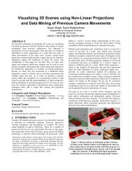
Fig. 1. Reference frames. Regions of interest were selected manually, and individual
point locations selected automatically using Shi and Tomasi’s method [22]. Note that,
in the first sequence, most points are clearly visible in only one reference frame. (Refer
to the electronic version of this paper to view the points in color.)
(a)
(b)
Frame 2 Frame 60 Frame 100
Fig. 2. (a) Rank-constrained tracking of the rigid sequence without outlier detection
(i.e. using τ = 0), using the reference frames shown in Figure 1(a). Tracks on occluded
portions of the face are consistently lost. (b) Robust, rank-constrained tracking applied
to the same sequence. Tracks are colored according to the average value of γ w,j,t for the
pixels in the track’s window: green for completely valid pixels, and red for all outliers.
4 Non-Rigid 3D Shape Reconstruction from Video
We now apply our framework to the case where 3D shape consists of both rigid
motion and non-rigid deformation, and show how to solve for the deforming
shape from video, while detecting outliers and solving for the shape and outlier
PDFs. Our approach builds on our previous algorithm for non-rigid structurefrom-motion
[5], which, as previously demonstrated on toy examples, yields much
better reconstructions than applying a user-defined regularization.

10 L. Torresani and A. Hertzmann
We assume that the nonrigid shape S t at time t can be described as a “shape
average” ¯S plus a linear combination of K basis shapes V k :
K∑
S t = Γ (z t ; ψ) = ¯S + V k z k,t (22)
k=1
where k indexes elements of z t and ψ = {¯S, V 1 , ..., V K }. The scalar weights z k,t
indicate the deformation in each frame t. Together, ¯S and V k are referred to as
the shape basis. The z t are Gaussian hidden variables with zero mean and unit
variance (p(z t ) = N (z t |0; I)). With z t treated as a hidden variable, this model
is a factor analyzer, and the distribution over shape p(S t ) is Gaussian. See [5]
for a more detailed discussion of this model. Scene points are viewed under
orthographic projection according to the model: Π(s j,t ; {R t , t t }) = R t s j,t + t t .
The imaging model is the same as described in Section 2.2. We encapsulate the
model in the parameter vector θ = {Ī, σ2 , τ, R 1 , ..., R T , t 1 , ..., t T , ¯S, V 1 , ..., V K }.
We optimize the VFE by alternating updates of each of the parameters. Each
update entails setting ∂F to zero with respect to each of the parameters; e.g. t t
is updated by solving ∂F
∂t t
= 0. The algorithm is given in the appendix.
Experiments. We tested our integrated 3D reconstruction algorithm on a challenging
video sequence of non-rigid human motion. The video consists of 660
frames recorded in our lab with a consumer digital video camera and contains
non-rigid deformations of a human torso. Although most of the features tracked
are characterized by distinctive 2D texture, their local appearance changes considerably
during the sequence due to occlusions, shape deformations, varying
illumination in patches, and motion blur. More than 25% of the frames contain
occluded features, due to arm motion and large torso rotations. 77 features
were selected automatically in the first frame using the criterion described by
Shi and Tomasi [22]. Figure 1(b) shows their initial locations in the reference
frame. The sequence was initially processed assuming K = 1 (corresponding
to rigid motion plus a single mode of deformation), and increased to K = 2
during optimization. Estimated positions of features with and without robustness
are shown in Figure 3. As shown in Figure 3(a), tracking without outlier
detection fails to converge to a reasonable result, even if initialized with
the results of the robust algorithm. 3D reconstructions from our algorithm
are shown in Figure 4(b). The resulting 3D shape is highly detailed, even for
occluded regions. For comparison, we applied robust rank-constrained tracking
to solve for maximum likelihood z t and θ, followed by applying the EM-
Gaussian algorithm [5] to the recovered point tracks. Although the results are
mostly reasonable, a few significant errors occur in an occluded region. Our algorithm
avoids these errors, because it optimizes all parameters directly with
respect to the raw image data. Additional results and visualizations are shown
at http://movement.stanford.edu/automatic-nr-modeling/

Automatic Non-Rigid 3D Modeling from Video 11
(a)
(b)
Frame 325 Frame 388 Frame 528
Fig. 3. (a) Rank-constrained tracking of the second sequence without outlier detection
fails to converge to a reasonable result. Here we show that, even when initialized with
the solution from the robust method, tracking without robustness causes the results to
degrade. (b) Robust, rank-constrained tracking applied to the same sequence. Tracks
are colored according to the average value of γ w,j,t for the pixels in the track’s window:
green for completely valid pixels, and red for all outliers.
(a)
(b)
Fig. 4. 3D reconstruction comparison. (a) Robust covariance-weighted factorization,
plus EM-Gaussian [5]. (b) Our result, using integrated non-rigid reconstruction. Note
that even occluded areas are accurately reconstructed by the integrated solution.
5 Discussion and future work
We have presented techniques for tracking and reconstruction from video sequences
that contain occlusions and other common violations of color constancy,
as well as complicated non-rigid shape and unknown system parameters. Previously,
tracking challenging footage with severe occlusions or non-rigid defor-

12 L. Torresani and A. Hertzmann
Fig. 5. Tracking and 3D reconstruction from a bullfight sequence, taken from the movie
Talk To Her. (The camera is out-of-focus in the second image).
mations could only be achieved with very strong shape and appearance models.
We have shown how to track such difficult sequences without prior knowledge
of appearance and dynamics.
We expect that these techniques can provide a bridge to very practical tracking
and reconstruction algorithms, by allowing one to model important variations
in detail without having to model all other sources of non-constancy. There are
a wide variety of possible extensions to this work, including: more sophisticated
lighting models (e.g. [23]), layer-based decomposition (e.g. [6]), and temporal
smoothness in motion and shape (e.g. [24, 5]).
It would be straightforward to handle true perspective projection for rigid
scenes in our framework, by performing bundle adjustment in the generalized
M-step. Our model could also be learned incrementally in a real-time setting
[16], although it would be necessary to bootstrap with a suitable initialization.
Acknowledgements. This work arose from discussions with Chris Bregler.
Thanks to Hrishikesh Deshpande for help with data capture, and to Kyros Kutulakos
for discussion. Portions of this work were performed while LT was visiting
New York University, and AH was at University of Washington. LT was supported
by ONR grant N00014-01-1-0890 under the MURI program. AH was
supported in part by UW Animation Research Labs, NSF grant IIS-0113007,
the Connaught Fund, and an NSERC Discovery Grant.
References
1. Irani, M.: Multi-Frame Correspondence Estimation Using Subspace Constraints.
Int. J. of Comp. Vision 48 (2002) 173–194
2. Torresani, L., Yang, D., Alexander, G., Bregler, C.: Tracking and Modeling Non-
Rigid Objects with Rank Constraints. In: Proc. CVPR. (2001)
3. Brand, M.: Morphable 3D models from video. In: Proc. CVPR. (2001)
4. Soatto, S., Yezzi, A.J.: DEFORMOTION: Deforming Motion, Shape Averages, and
the Joint Registration and Segmentation of Images. In: Proc. ECCV. Volume 3.
(2002) 32–47
5. Torresani, L., Hertzmann, A., Bregler, C.: Learning Non-Rigid 3D Shape from 2D
Motion. In: Proc. NIPS 16. (2003) To appear.
6. Jojic, N., Frey, B.: Learning Flexible Sprites in Video Layers. In: Proc. CVPR.
(2001)
7. Horn, B.K.P.: Robot Vision. McGraw-Hill, New York, NY (1986)
8. Lucas, B.D., Kanade, T.: An iterative image registration technique with an application
to stereo vision. In: Proc. 7th IJCAI. (1981)

Automatic Non-Rigid 3D Modeling from Video 13
9. Irani, M., Anandan, P.: About Direct Methods. In: Vision Algorithms ’99. (2000)
267–277 LNCS 1883.
10. Bregler, C., Hertzmann, A., Biermann, H.: Recovering Non-Rigid 3D Shape from
Image Streams. In: Proc. CVPR. (2000)
11. Torresani, L., Bregler, C.: Space-Time Tracking. In: Proc. ECCV. Volume 1.
(2002) 801–812
12. Forsyth, D.A., Ponce, J.: Computer Vision: A Modern Approach. Prentice Hall
(2003)
13. Dellaert, F., Seitz, S.M., Thorpe, C.E., Thrun, S.: EM, MCMC, and Chain Flipping
for Structure from Motion with Unknown Correspondence. Machine Learning 50
(2003) 45–71
14. Black, M.J., Anandan, P.: The robust estimation of multiple motions: Parametric
and piecewise-smooth flow fields. Computer Vision and Image Understanding 63
(1996) 75–104
15. Jepson, A., Black, M.J.: Mixture models for optical flow computation. In: Proc.
CVPR. (1993) 760–761
16. Jepson, A.D., Fleet, D.J., El-Maraghi, T.F.: Robust Online Appearance Models
for Visual Tracking. IEEE Trans. PAMI 25 (2003) 1296–1311
17. Wang, J.Y.A., Adelson, E.H.: Representing moving images with layers. IEEE
Trans. Image Processing 3 (1994) 625–638
18. Weiss, Y., Adelson, E.H.: Perceptually organized EM: A framework for motion
segmentation that combines information about form and motion. Technical Report
TR 315, MIT Media Lab Perceptual Computing Section (1994)
19. Jordan, M.I., Ghahramani, Z., Jaakkola, T.S., Saul, L.K.: An introduction to variational
methods for graphical models. In Jordan, M.I., ed.: Learning in Graphical
Models. Kluwer Academic Publishers (1998)
20. Morris, D.D., Kanade, T.: A Unified Factorization Algorithm for Points, Line
Segments and Planes with Uncertainty Models. In: Proc. ICCV. (1998) 696–702
21. Tomasi, C., Kanade, T.: Shape and motion from image streams under orthography:
A factorization method. Int. J. of Computer Vision 9 (1992) 137–154
22. Shi, J., Tomasi, C.: Good Features to Track. In: Proc. CVPR. (1994) 593–600
23. Zhang, L., Curless, B., Hertzmann, A., Seitz, S.M.: Shape and Motion under
Varying Illumination: Unifying Structure from Motion, Photometric Stereo, and
Multi-view Stereo. In: Proc. ICCV. (2003) 618–625
24. Gruber, A., Weiss, Y.: Factorization with Uncertainty and Missing Data: Exploiting
Temporal Coherence. In: Proc. NIPS 16. (2003) To appear.
A
Non-rigid reconstruction algorithm
The non-rigid reconstruction algorithm of Section 4 alternates between optimizing
the VFE with respect to each of the unknowns. The linearization in
Equation 14 is used to make these updates closed-form. This linearization also
means that the distribution q(z t ) is Gaussian. We represent it with the variables
µ t ≡ E q(zt)[z t ] and φ t ≡ E q(zt)[z t z T t ].
We additionally define ˜H = [vec(¯S), vec(V 1 ), ..., vec(V K )] and ˜z t = [1, z T t ] T ;
hence, S t = ˜H˜z t . Additionally, we define ˜µ t = E[˜z t ] and ˜φ = E[˜z t˜z T t ]. ˜H j refers
to the rows of ˜H j corresponding to the j-th scene point (i.e. s j,t = ˜H j˜z t ).

14 L. Torresani and A. Hertzmann
A.1 Outlier variables
We first note the following identity, which gives the expected reconstruction error
for a pixel, taken with respect to q(z t ):
E q(zt)[(I w (p t,j ) − Īw,j) 2 ] = ∇I T w (R t ˜H j ˜φt ˜H T j R T t + 2R t ˜H j ˜µ t t T t + t t t T t )∇I w −
2(∇I T w p 0 j,t + Īw,j − I w (p 0 j,t))∇I T w (R t ˜H j ˜µ t + t t )
(∇I T w p 0 j,t + Īw,j − I w (p 0 j,t)) 2 (23)
We can then use this identity to evaluate the update steps for the outlier
probabilities γ w,j,t and the noise variance σ 2 according to Equation 13 and 19,
respectively.
A.2 Shape parameter updates
The following shape updates are very similar to our previous algorithm [5], but
with a specified covariance matrix for each track. We combine the virtual tracks
for each frame into a single vector f t = [ˆp T 1,t, ..., ˆp T J,t ]T ; this vector has covariance
E −1
t , which is a block-diagonal matrix containing e −1
j,t along the diagonal. We
also define ¯f t = vec(R t¯S), and stack the J copies of the 2D translation as T t =
[t T t , t T t , ...t T t ] T .
Shape may be thus updated with respect to the virtual tracks as:
M t ← [vec(R tV 1), ..., vec(R tV K)] (24)
β ← M T t (M tM T t + E −1
t ) −1 (25)
µ t ← β(f t − ¯f t − T t), ˜µ t ← [1, µ T t ] T (26)
[ ]
φ t ← I − βM t + µ tµ T 1 µ
T
t , ˜φ ← t
(27)
µ t φ t
( −1 ( )
∑ ∑
vec( ˜H) ← (˜φ t ⊗ ((I ⊗ R T t )E t(I ⊗ R t))))
vec (I ⊗ R t) T E t(f t − T t)˜µ T t
t
t
( ) −1
∑ ∑
∑
t t ← e t,j e t,j(f tj − R t(¯s j + V kj µ tk )) (29)
j
j
k
∑
∑
R t ← arg min || (( ˜H j ˜φ t ˜H T j ) ⊗ e t,j)vec(R t) − vec( (e t,j(f tj − t t)˜µ T ˜H t T j ))||
R t
j
where the symbol ⊗ denotes Kronecker product. Note that Equation 28 updates
the shape basis ¯S and V; conjugate gradient is used for this update. The rotation
matrix R t is updated by linearizing the objective in Equation 30 with exponential
maps, and solving for an improved estimate.
j
(28)
(30)