[pdf]Climate profile of India - India Meteorological Department

Government of India
Ministry of Earth Sciences
India Meteorological Department
Met Monograph No. Environment Meteorology-01/2010
CLIMATE PROFILE OF INDIA
S. D. Attri and Ajit Tyagi
1
0.8
9 POINT BINOMIAL FILTER
0
TREND=+0.56 C/100 YEARS
Annual Mean Temp Anomalies (°C)
0.6
0.4
0.2
0
-0.2
-0.4
-0.6
-0.8
1901 1910 1919 1928 1937 1946 1955 1964 1973 1982 1991 2000 2009
Y E R S A
2010

Met Monograph No.
Environment Meteorology-01/2010
CLIMATE PROFILE OF INDIA
Contribution to the
Indian Network of Climate Change Assessment
(NATIONAL COMMUNICATION-II)
Ministry of Environment and Forests
S D Attri and Ajit Tyagi
India Meteorological Department
Ministry of Earth Sciences
New Delhi
2010

Copyright
© 2010 by India Meteorological Department
All Rights Reserved.
Disclaimer and Limitations
IMD is not responsible for any errors and omissions. The geographical
boundaries shown in the publication do not necessarily correspond to the
political boundaries.
Published in India
By
Environment Monitoring and Research Centre,
India Meteorological Department, Lodi Road, New Delhi- 110003 (India)
Phone: 91-11-24620701
Email: met_emu@yahoo.com

PREFACE
The beginnings of meteorology in India can be traced to ancient times from
the philosophical writings of the Vedic period, contain serious discussion about the
processes of cloud formation and rain and the seasonal cycles caused by the
movement of earth round the sun. But, the Modern Meteorology is regarded to have
had its firm scientific foundation in the 17th century after the invention of
thermometer, barometer and the formulation of laws governing the behaviour of
atmospheric gases. India is fortunate to have some of the oldest meteorological
observatories of the world like those at Calcutta (now Kolkata) in 1785 and Madras
(now Chennai) in 1796 for studying the weather and climate of India
India Meteorological Department (IMD) has progressively expanded its
infrastructure for meteorological observations, communications, forecasting and
weather services and it has concurrently contributed to scientific growth since its
inception in 1875. One of the first few electronic computers introduced in the country
was provided to IMD for scientific applications in meteorology. India was the first
developing country in the world to have its own geostationary satellite, INSAT, for
continuous weather monitoring of this part of the globe and particularly for cyclone
warning. It has ventured into new areas of application and service, and steadily built
upon its infra-structure during its history of 135 years. It has simultaneously nurtured
the growth of meteorology and atmospheric science in India for sectoral services.
Systematic observation of basic climate, environmental and oceanographic data is
vital to capture past and current climate variability.
IMD has provided climatic observations and products to the national
requirements including National Communication (NATCOM). To meet the future
need, it is in process of augmenting its weather and climate-related observation
systems that underpins analytical and predictive capability which is critical for
minimising extreme climate variability impacts.
I am hopeful that this publication on “Climate Profile of India” will contribute to
the “India’s National Communication-II” to be submitted to UNFCCC next year. The
publication is based on the work mainly carried out by IMD scientists. I extend my
sincere thanks to Sh. A K Bhatnagar, Dr A Mazumdar, Dr Y E A Raj,
Sh B. Mukhopadhyay, Sh N Y Apte, Dr Medha Khole, Dr M Mohapatra,
Dr A K Srivastava and Dr J Sarkar for providing requisite inputs.
October 2010
New Delhi
Ajit Tyagi
Director General of Meteorology

INDIA METEOROLOGICAL DEPARTMENT
DOCUMENT AND DATA CONTROL SHEET
1 Document title Climate Profile of India
2 Document type Met Monograph
3 Issue No. Environment Meteorology-01/2010
4 Issue date October 2010
5 Security Classification Unclassified
6 Control Status Uncontrolled
7 No. of Pages 122
8 No. figures 39
9 No. of reference 62
10 Distribution Unrestricted
11 Language English
12 Authors S D Attri and Ajit Tyagi
13 Originating
EMRC
Division/Group
14 Reviewing and
DGM
Approving Authority
15 End users Ministries / Departments of Central and State
Governments, Research organisations, INCCA
(NATCOM), Scientific community, Public etc.
16 Abstract Normal climatic pattern and long term trends
over India during last more than 100 years have
been presented here. The publication contains
studies with latest data on various aspects of
important weather / climate systems viz.
Monsoons, Cyclone, Drought, Floods and
observational weather / climate mechanism in
the country. Status and trends in parameters of
atmospheric environment viz. radiation, ozone,
precipitation chemistry etc has been depicted.
The publication is also intended to provide
requisite details for Indian Network of Climate
Change Assessment (INCCA) to address climate
change issues.
17 Key words Climate Change, Cyclone, Monsoon, Drought,
Flood, Environment

CLIMATE PROFILE OF INDIA
CONTENTS
1. Climate profile 1-8
2. Systematic observations 9-16
3. Climate change scenario 17-32
4. Behaviour of Monsoons 33-54
5. Floods 55-61
6. Tropical cyclones 62-89
7. Drought 90-105
8. Environmental status in India 106-117
References 118-122

Chapter - I
CLIMATE PROFILE
1. Introduction
India is home to an extraordinary variety of climatic regions, ranging from
tropical in the south to temperate and alpine in the Himalayan north, where elevated
regions receive sustained winter snowfall. The nation's climate is strongly influenced
by the Himalayas and the Thar Desert. The Himalayas act as a barrier to the
frigid katabatic winds flowing down from Central Asia keeping the bulk of the Indian
subcontinent warmer than most locations at similar latitudes. As such, land areas in
the north of the country have a continental climate with severe summer conditions
that alternates with cold winters when temperatures plunge to freezing point. In
contrast are the coastal regions of the country, where the warmth is unvarying and
the rains are frequent.
The country is influenced by two seasons of rains, accompanied by seasonal
reversal of winds from January to July. During the winters, dry and cold air blowing
from the northerly latitudes from a north-easterly direction prevails over the Indian
region. Consequent to the intense heat of the summer months, the northern Indian
landmass becomes hot and draws moist winds over the oceans causing a reversal of
the winds over the region which is called the summer or the south-west monsoon
This is most important feature controlling the Indian climate because about 75% of
the annual rainfall is received during a short span of four months (June to
September). Variability in the onset, withdrawal and quantum of rainfall during the
monsoon season has profound impacts on water resources, power generation,
agriculture, economics and ecosystems in the country. The variation in climate is
perhaps greater than any other area of similar size in the world. There is a large
variation in the amounts of rainfall received at different locations. The average
annual rainfall is less than 13 cm over the western Rajasthan, while at Mausiram in
the Meghalaya has as much as 1141 cm. The rainfall pattern roughly reflects the
different climate regimes of the country, which vary from humid in the northeast
1

(about 180 days rainfall in a year), to arid in Rajasthan (20 days rainfall in a year). So
significant is the monsoon season to the Indian climate, that the remaining season
are often referred relative to the monsoon.
The rainfall over India has large spatial as well as temporal variability. A
homogeneous data series has been constructed for the period 1901-2003 based on
the uniform network of 1476 stations and analyzed the variability and trends of
rainfall. Normal rainfall (in cm) pattern of the country for the four seasons and annual
are depicted in Fig 1 and Fig 2 respectively. Normal monsoon rainfall more than
150cm is being observed over most parts of northeast India, Konkan & Goa. Normal
monsoon rainfall is more than 400cm over major parts of Meghalaya. Annual rainfall
is more than 200 cm over these regions.
For the country as whole, mean monthly rainfall during July (286.5 mm) is
highest and contributes about 24.2% of annual rainfall (1182.8 mm). The mean
rainfall during August is slightly lower and contributes about 21.2% of annual rainfall.
June and September rainfall are almost similar and contribute 13.8% and 14.2% of
annual rainfall, respectively. The mean south-west monsoon (June, July, August &
September) rainfall (877.2 mm) contributes 74.2% of annual rainfall (1182.8 mm).
Contribution of pre-monsoon (March, April & May) rainfall and post-monsoon
(October, November & December) rainfall in annual rainfall is mostly the same
(11%). Coefficient of variation is higher during the months of November, December,
January and February.
India is characterised by strong temperature variations in different seasons
ranging from mean temperature of about 10°C in winter to about 32 °C in summer
season (Fig 3). Details of weather along with associated systems during different
seasons are presented as under:
1.1 Winter Season / Cold Weather Season (January and February)
India Meteorological Department (IMD) has categorised the months of
January and February in winter season. However, December can be included in this
season for north-western parts of the country. This season starts in early December
2

associated with clear skies, fine weather, light northerly winds, low humidity and
temperatures, and large daytime variations of temperature . The cold air mass
extending from the Siberian region, has profound influence on the Indian
subcontinent (at least all of the north and most of central India) during these months.
The mean air temperatures increase from north to south up to 17°N, the decrease
being sharp as one moves northwards in the north-western parts of the country. The
mean temperatures vary from 14 °C to 27°C during January. The mean daily
minimum temperatures range from 22 °C in the extreme south, to 10 °C in the
northern plains and 6 °C in Punjab. The rains during this season generally occur
over the western Himalayas, the extreme north-eastern parts, Tamil Nadu and
Kerala. Western disturbances and associated trough in westerlies are main rain
bearing system in northern and eastern parts of the country.
1.2 Pre-monsoon season/ Summer season/ Hot weather season/
Thunderstorm season (March, April and May)
The temperatures start to increase all over the country in March and by April,
the interior parts of the peninsula record mean daily temperatures of 30-35 °C.
Central Indian land mass becomes hot with daytime maximum temperatures
reaching about 40°C at many locations. Many stations in Gujarat, North
Maharashtra, Rajasthan and North Madhya Pradesh exhibit high day-time and low
night-time temperatures during this season. The range of the daytime maximum and
night-time minimum temperatures in found more than 15 °C at many stations in
these States. Maximum temperatures rise sharply exceeding 45 °C by the end of
May and early June resulting in harsh summers in the north and north-west regions
of the country. However, weather remains mild in coastal areas of the country owing
to the influence of land and sea breezes.
The season is characterised by cyclonic storms, which are intense low
pressure systems over hundreds to thousands of kilometres associated with
surface winds more than 33 knots over the Indian seas viz. Bay of Bengal and the
Arabian Sea. These systems generally move towards a north-westerly direction and
some of them recurve to northerly or northeasterly path. Storms forming over the
3

Bay of Bengal are more frequent than the ones originating over the Arabian Sea. On
an average, frequency of these storms is about 2.3 per year.
Weather over land areas is influenced by thunderstorms associated with rain
and sometimes with hail in this season. Local severe storms or violent thunderstorms
associated with strong winds and rain lasting for short durations occur over the
eastern and north eastern parts over Bihar, West Bengal, and Assam. They are
called norwesters or “Kal Baisakhis” as generally approach a station from the
northwesterly direction. Thunderstorms are also observed over central India
extending to Kerala along wind-discontinuity lines. Hot and dry winds accompanied
with dust winds (“andhis” ) blow frequently over the plains of north-west India.
1.3 South-west Monsoon/ Summer Monsoon (June, July, August and
September)
The SW monsoon is the most significant feature of the Indian climate. The
season is spread over four months, but the actual period at a particular place
depends on onset and withdrawal dates. It varies from less than 75 days over
West Rajasthan, to more than 120 days over the south-western regions of the
country contributing to about 75% of the annual rainfall.
The onset of the SW monsoon normally starts over the Kerala coast, the
southern tip of the country by 1 June, advances along the Konkan coast in early
June and covers the whole country by middle of July. However, onset occurs
about a week earlier over islands in the Bay of Bengal. The monsoon is a special
phenomenon exhibiting regularity in onset and distribution within the country, but
inter-annual and intrannual variations are observed. The monsoon is influenced by
global and local phenomenon like El Nino, northern hemispheric temperatures, sea
surface temperatures, snow cover etc. The monsoonal rainfall oscillates between
active spells associated with widespread rains over most parts of the country and
breaks with little rainfall activity over the plains and heavy rains across the foothills of
the Himalayas. Heavy rainfall in the mountainous catchments under ‘break’
conditions results flooding over the plains. However, very uncomfortable weather
due to high humidity and temperatures is the feature associated with the Breaks.
4

Cyclonic systems of low pressure called ‘monsoon depressions’ are formed
in the Bay of Bengal during this season. These systems generally form in the
northern part of the Bay with an average frequency of about two to three per month
and move in a northward or north-westward direction, bringing well-distributed
rainfall over the central and northern parts of the country. The distribution of rainfall
over northern and central India depends on the path followed by these
depressions. SW monsoon current becomes feeble and generally starts
withdrawing from Rajasthan by 1 st September and from north-western parts of India
by 15 th September. It withdraws from almost all parts of the country by 15 th October
and is replaced by a northerly continental airflow called North-East Monsoon. The
retreating monsoon winds cause occasional showers along the east coast of Tamil
Nadu, but rainfall decreases away from coastal regions.
1.4 Post-monsoon or Northeast monsoon or Retreating SW Monsoon
season (October, November and December)
North-East (NE) monsoon or Post-monsoon season is transition season
associated with the establishment of the north-easterly wind regime over the Indian
subcontinent. Meteorological subdivisions namely Coastal Andhra Pradesh
Rayalaseema , Tamil Nadu, Kerala and South Interior Karnataka receive good
amount of rainfall accounting for about 35% of their annual total in these months.
Many parts of Tamil Nadu and some parts of Andhra Pradesh and Karnataka receive
rainfall during this season due to the storms forming in the Bay of Bengal. Large
scale losses to life and property occur due to heavy rainfall, strong winds and storm
surge in the coastal regions. The day temperatures start falling sharply all over the
country. The mean temperatures over north-western parts of the country show
decline from about 38°C in October to 28°C in November. Decrease in humidity
levels and clear skies over most parts of north and central India after mid-October
are characteristics features of this season (NATCOM 2004, IMD 2010).
5

(a)
(b)
(c)
(d)
Fig 1: Normal rainfall pattern (cm) during (a) Winter (b) Pre-monsoon (c) Monsoon and
(d) Post-Monsoon seasons for the period 1941-90
6

Fig 2: Annual normal rainfall pattern (cm) during 1941-90
7

Fig. 3: Seasonal temperature distribution over India
8

Chapter - II
SYSTEMATIC OBSERVATIONS
Agriculture based economy under favourable climatic conditions of the
summer monsoon has necessitated a closer linkage with weather and climate since
the Vedic period. Ancient Indian literature by Varahmihir, the ‘Brihat-Samhita’, is an
example of ancient Indian weather research. Modernized meteorological
observations and research in India was initiated more than 200 years ago, since
1793, when the first Indian meteorological observatory was set up at Madras (now
Chennai). IMD was formally established in 1875 with a network of about 90 weather
observatories for systematic observation and research. Agricultural-meteorology
directorate was created in 1932 to further augment the observation network. Many
data and research networks have been added during the 135 years for climatedependent
sectors, such as agriculture, forestry, and hydrology, rendering a modern
scientific background to atmospheric science in India. The inclusion of the latest data
from satellites and other modern observation platforms, such as Automated Weather
Stations (AWS), and ground-based remote-sensing techniques, has strengthened
India’s long-term strategy of building up a self-reliant climate data bank for specific
requirements, and also to fulfill international commitments of data exchange for
weather forecasting and allied research activities. The latest observational network in
depicted in Table 1.
2.1 Institutional arrangements
The Ministry and Environment and Forests (MoEF), Ministry of Earth
Sciences (MoES), Ministry of Science and Technology (MST), Ministry of Agriculture
(MoA), Ministry of Water Resources (MWR), Ministry of Human Resource
Development (MHRD), Ministry of Nonconventional Energy (MNES), Ministry of
Defence (MoD), Ministry of Health and Family welfare (MoHFW), Indian Space
Research Organization (ISRO) and India Meteorological Department (IMD) promote
and undertake climate and climate change-related research in the country. The
MoES, MoEF, MST, MHRD and MOA also coordinate research and observations in
9

many premier national research laboratories and universities. The IMD possesses a
vast weather observational network and is involved in regular data collection basis,
data bank management, research and weather forecasting for national policy needs.
2.2 Atmospheric monitoring
There are 25 types of atmospheric monitoring networks that are operated and
coordinated by the IMD. This includes meteorological/climatological, environment/ air
pollution and other specialized observation of atmospheric trace constituents. It
maintains 559 surface meteorological observatories, about 35 radio-sonde and 64
pilot balloon stations for monitoring the upper atmosphere. Specialized observations
are made for agro-meteorological purposes at 219 stations and radiation parameters
are monitored at 45 stations. There are about 70 observatories that monitor current
weather conditions for aviation. Although, severe weather events are monitored at
all the weather stations, the monitoring and forecasting of tropical cyclones is
specially done through three Area Cyclone Warning Centres (Mumbai, Chennai, and
Kolkata) and three cyclone warning centres (Ahmedabad, Vishakhapatnam and
Bhubaneswar), which issue warnings for tropical storms and other severe weather
systems affecting Indian coasts. Storm and cyclone detections radars are installed
all along the coast and some key inland locations to observe and forewarn severe
weather events, particularly tropical cyclones. The radar network is being upgraded
by modern Doppler Radars, with enhanced observational capabilities, at many
locations.
In another atmospheric observation initiative, the IMD established 10 stations
in India as a part of World Meteorological Organization’s (WMO) Global Atmospheric
Watch (GAW, formerly known as Background Air Pollution Monitoring Network or
BAPMoN). The Indian GAW network includes Allahabad, Jodhpur, Kodaikanal,
Minicoy, Mohanbari, Nagpur, Port Blair, Pune, Srinagar and Visakhapatnam.
Atmospheric turbidity is measured using hand-held Volz’s Sunphotometers at
wavelength 500 nm at all the GAW stations. Total Suspended Particulate Matter
(TSPM) is measured for varying periods at Jodhpur using a High Volume Air
Sampler. Shower-wise wet only precipitation samples are collected at all the GAW
stations using specially designed wooden precipitation collectors fitted with stainless
10

steel or polyethylene funnel precipitation collectors. After each precipitation event,
the collected water is transferred to a large storage bottle to obtain a monthly
sample. Monthly mixed samples collected from these stations are sent to the
National Chemical Laboratory, Pune, where these are analyzed for pH, conductivity,
major cations (Ca, Mg, Na, K, NH 4 +) and major anions (SO 4 2-, NO 3 -, Cl-).
The IMD established the glaciology Study Research Unit in Hydromet.
Directorate in 1972. This unit has been participating in glaciological expedition
organized by the GSI and the DST. The unit was established for the: (a)
determination of the natural water balance of various river catchment areas for better
planning and management of the country’s water resources; (b) snow melt run-off
and other hydrological forecasts; (c) reservoir regulation; (d) better understanding of
climatology of the Himalaya; and (e) basic research of seasonal snow cover and
related phenomena. The IMD has established observing stations over the Himalayan
region to monitor weather parameters over glaciers.
In view of the importance of data in the tropical numerical weather prediction,
IMD has been in the process of implementing a massive modernization programme
for upgrading and enhancing its observation system. It is establishing 550 AWS out
of which about 125 will have extra agricultural sensors like solar radiation, soil
moisture and soil temperature, 1350 Automatic Rain Gauge (ARG) stations and 10
GPS in 2009 and will increase these to 1300, 4000 and 40, respectively . In
addition to this, a network of 55 Doppler Weather Radar has been planned of which
12 are to be commissioned in the first phase. DWR with the help of algorithms can
detect and diagnose weather phenomena, which can be hazardous for agriculture,
such as hail, downbursts and squall. A new satellite INSAT-3D is scheduled to be
launched during 2011. INSAT-3D will usher a quantum improvement in satellite
derived data from multi spectral high resolution imagers and vertical sounder. In
addition to above, IMD is also planning to install wind profilers and radiometer to get
upper wind and temperature data.
It is also augmenting its monitoring capability of the parameters of
atmospheric environment. Trace gases, precipitation chemistry and aerosols will be
monitored in the country on a long term basis at 2 baseline and 4 grab sample
11

GHG monitoring stations, Aerosol monitoring at 14 stations using sky radiometers,
Black carbon measurement at 4 stations using aethelometers, Ozone
measurements in NE and Port Blair in addition to existing stations in India and
Antarctica, Turbidity and Rain Water chemistry at 11 stations and Radiation
measurements at 45 stations. The data will be monitored and exchanged globally as
per GAW / WMO protocols and quality control will be ensured as per international
standards. Such data will be used in C-cycle models to accurately estimate radiation
forcing and quantify source and sink potential for policy issues under UN framework.
The IMD, in collaboration with the NPL plays an important role for climate
change-related long-term data collection at the Indian Antarctic base-Maitri.
Continuous surface meteorological observations for about 22 years are now
available for Schirmacher Oasis with National Data Centre of IMD.
The IMD collects meteorological data over oceans by an establishment of
cooperation fleet of voluntary observing ships (VOF) comprising merchant ships of
Indian registry, some foreign merchant vessels and a few ships of the Indian Navy.
These ships, while sailing on the high seas, function as floating observatories.
Records of observations are passed on to the IMD for analysis and archival.
2.3 Data archival and exchange
The tremendous increase in the network of observatories resulted in the
collection of a huge volume of data. The IMD has climatological records even for the
period prior to 1875, when it formally came into existence. This data is digitized,
quality controlled and archived in electronic media at the National Data Centre,
Pune. The current rate of archival is about three million records per year. At present,
the total holding of data is about 9.7 billion records. They are supplied to universities,
industry, research and planning organizations. The IMD prepared climatological
tables and summaries/ atlases of surface and upper-air meteorological parameters
and marine meteorological summaries. These climatological summaries and
publications have many applications in agriculture, shipping, transport, water
resources and industry.
12

The IMD has its own dedicated meteorological telecommunication network
with the central hub at New Delhi. Under the WWW Global Telecommunication
System, New Delhi functions as a Regional Telecommunication Hub (RTH) on the
main telecommunication network. This centre was automated in early 1976, and is
now known as the National Meteorological Telecommunication Centre (NMTC), New
Delhi. Within India, the telecommunication facility is provided by a large network of
communication links. The websites of IMD viz. http://www.imd.gov.in /
http://www.mausam.gov.in operational from 1 June, 2000 contains dynamically
updated information on all-India weather and forecasts, special monsoon reports,
satellite cloud pictures updated every three hours, Limited Area Model (LAM), Global
Circulation Model (GCM) generated products and prognostic charts, special weather
warnings, tropical cyclone information and warnings, weekly and monthly rainfall
distribution maps, earthquake reports, etc. It also contains a lot of static information,
including temperature and rainfall normal over the country; publications, data
archival details, monitoring networks and a brief overview of the activities and
services rendered by IMD.
2.4 Augmentation of Weather and Climate forecasting capabilities (short,
medium and long range)
In view of growing operational requirements from various user agencies, IMD
has embarked on a seamless forecasting system covering short range to extended
range and long range forecasts. Such forecasting system is based on hierarchy of
Numerical Weather Prediction (NWP) models. For a tropical country like India where
high impact mesoscale convective events are very common weather phenomena, it
is necessary to have good quality high density observations both in spatial and
temporal scale to ingest into assimilation cycle of a very high resolution nonhydrostatic
mesoscale model. A major problem related to skill of NWP models in the
tropics is due to sparse data over many parts of the country and near absence of
data from oceanic region.
Data from AWSs, ARGs, DWRs, INSAT-3D and wind profilers are available in
real time for assimilation in NWP models. A High Power Computing (HPC) system
with 300 terabyte storage has been installed at NWP Centre at Mausam Bhavan. All
13

the systems have started working in an integrated manner in conjunction with other
systems, such as all types of observation systems, AMSS, CIPS, HPCS, synergy
system etc., in a real-time and have greatly enhanced IMD capability to run global
and regional models and produce indigenous forecast products in different time
scales. It has also started running a number of global and regional NWP models in
the operational mode . IMD also makes use of NWP Global model forecast products
of other operational centres, like NCMRWF T-254, ECMWF, JMA, NCEP, WRF and
UKMO to meet the operational requirements of day to day weather forecasts. Very
recently, IMD has implemented a multimodel ensemble (MME) based district level
five days quantitative forecasts in medium range.
Climate-related risks are likely to increase in magnitude and frequency in
future. There is need to prioritize actions to improve monitoring of such extremes
and refine models for their prediction and projection in longer scale. New levels of
integrated efforts like Global Framework for Climate Services/ National Framework
for Climate Services (GFCS/NFCS) are required to strengthen climate research at
existing and newer institutions to:
• Develop improved methodologies for the assessment of climate impacts on
natural and human system
• Characterize and model climate risk on various time and space scales
relevant to decision-making and refine climate prediction skills
• Enhance spatial resolution of climate predictions, including improvements in
downscaling and better regional climate models
• Improve climate models to represent the realism of complex Earth system
processes and their interactions in the coupled system
• Develop a better understanding of the linkages between climatic regimes and
the severity and frequency of extreme events
• Enable progress in improving operational climate predictions and streamlining
the linkages between research and operational service providers.
IMD is taking initiatives for creation of Indian Climate Observation System
(ICOS) to support such services in long run.
14

A dynamical statistical technique is developed and implemented for the realtime
cyclone genesis and intensity prediction. Numbers of experiments are carried
out for the processing of DWR observations to use in nowcasting and mesoscale
applications. The procedure is expected to be available in operational mode soon.
Impact of INSAT CMV in the NWP models has been reported in various studies.
Various multi-institutional collaborative forecast demonstration projects such as,
Dedicated Weather Channel, Weather Forecast for Commonwealth Games 2010,
Land falling Cyclone, Fog Prediction etc. are initiated to strengthen the forecasting
capabilities of IMD.
15

Table 1
Atmospheric monitoring networks
1 Surface observatories 559
2 Pilot balloon observatories 65
3 RS/RW observatories 3
4 Aviation current weather observatories 71
6 Storm detecting radar stations 17
7 Cyclone detection radar stations 10
8 High-wind recording stations 4
9 Stations for receiving cloud pictures from satellites
a Low-resolution cloud pictures 7
b High-resolution cloud pictures 1
c INSAT-IB cloud pictures(SDUC stations) 20
d APT Stations in Antarctica 1
e AVHRR station 1
10 Data Collection Platforms through INSAT 100
11 Hydro-meteorological observatories 701
a Non-departmental rain gauge stations
i Reporting 3540
ii Non-reporting 5039
b Non-departmental glaciological observations (non-reporting)
i Snow gauges 21
ii Ordinary rain gauges 10
iii Seasonal snow poles 6
12 Agro-meteorological observatories 219
13 Evaporation stations 222
14 Evapotranspiration stations 39
15 Seismological observatories 58
16 Ozone monitoring
a Total ozone and Umkehr observatories 5
b Ozone-sonde observatories 3
c Surface ozone observatories 6
17 Radiation observatories
a Surface 45
b Upper air 8
18 Atmospheric electricity observatories 4
19 a Background pollution observatories 10
b Urban Climatological Units 2
c Urban Climatological Observatories 13
20 Ships of the Indian voluntary observing fleet 203
21 Soil moisture recording stations 49
22 Dew-fall recording stations 80
23 AWS 550
24 ARG 1300
25 GPS 10
16

Chapter – III
CLIMATE CHANGE SCENARIO
India Meteorological Department (IMD) maintains a well distributed network of
more than 500 stations in the country for more than a century. The salient findings
of the IMD studies (IMD Annual Climate Summary, 2009, Tyagi and Goswami,
2009, Attri 2006) are summarized as under:
3.1 Temperature
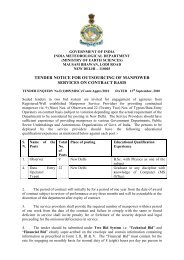
Analysis of data for the period 1901-2009 suggests that annual mean
temperature for the country as a whole has risen by 0.56 0 C (Fig 4) over the period. It
may be mentioned that annual mean temperature has been generally above normal
(normal based on period, 1961-1990) since 1990. This warming is primarily due to
rise in maximum temperature across the country, over larger parts of the data set
(Fig 5). However, since 1990, minimum temperature is steadily rising (Fig 6) and rate
of its rise is slightly more than that of maximum temperature (IMD Annual Climate
Summary, 2009). Warming trend over globe of the order of 0.74 0 C has been
reported by IPCC (2007)
Spatial pattern of trends in the mean annual temperature (Fig 7) shows
significant positive (increasing) trend over most parts of the country except over
parts of Rajasthan, Gujarat and Bihar, where significant negative (decreasing) trends
were observed (IMD Annual Climate Summary, 2009).
Season wise, maximum rise in mean temperature (Fig 8) was observed
during the Post-monsoon season (0.77 0 C) followed by winter season (0.70 0 C), Premonsoon
season (0.64 0 C) and Monsoon season (0.33 0 C). During the winter season,
since 1991, rise in minimum temperature is appreciably higher than that of maximum
temperature over northern plains. This may be due to pollution leading to frequent
occurrences of fog.
17

Upper air temperatures have shown an increasing trend in the lower
troposphere and this trend is significant at 850 hPa level, while decreasing trend (not
significant) was observed in the upper troposphere (Kothawale and.Rupa Kumar,
2002).
3.2 Precipitation Trends
The country as a whole, the all India annual and monsoon rainfall for the
period 1901-2009 do not show any significant trend (Fig. 9a & 9b). Similarly rainfall
for the country as whole for the same period for individual monsoon months also
does not show any significant trend. The alternating sequence of multi-decadal
periods of thirty years having frequent droughts and flood years are observed in the
all India monsoon rainfall data. The decades 1961-70, 1971-80 and 1981-90 were
dry periods. The first decade (1991-2000) in the next 30 years period already
experienced wet period.
However, during the winter season, rainfall is decreasing in almost all the subdivisions
except for the sub-divisions Himachal Pradesh, Jharkhand and Nagaland,
Manipur, Mizoram & Tripura. Rainfall is decreasing over most parts of the central
India during the pre-monsoon season. However during the post-monsoon season,
rainfall is increasing for almost all the sub-divisions except for the nine sub-divisions
(Fig 10).
The analysis for the monthly rainfall series of June, July, August, and
September (% variation) for all the 36 subdivisions (Guhathakurta, P. and Rajeevan
2008) shows significant variations on the regional scale (Fig. 11) which are
summarized as under:
• June rainfall has shown increasing trend for the western and southwestern
parts of the country whereas decreasing trends are observed for the central
and eastern parts of the country. Its contribution to annual rainfall is
increasing in 19 subdivisions and decreasing in the remaining 17
subdivisions.
18

• The contribution of July rainfall is decreasing in central and west peninsular
India (significantly in South interior Karnataka (95%), East M.P.(90%)
Vidarbha (90%), Madhya Maharashtra (90%), Marathwada (90%), Konkan &
Goa (90%), and North interior Karnataka (90%)), but has increased
significantly in the northeastern parts of the country
• In August, four (ten) subdivisions have shown decreasing (increasing) trends in
rainfall. It has increased significantly (at 95% significance level) over the
subdivisions Konkan and Goa, Marathwada, Madhya Maharashtra, Vidarbha,
West M.P., Telangana and west U.P.
• September rainfall is increasing significantly (at 95% level of significance) in
Gangetic West Bengal and decreasing significantly (at 90% level of
significance) for the sub-divisions Marathwada, Vidarbha and Telangana.
During the season, three subdivisions viz. Jharkhand (95%), Chattisgarh
(99%), Kerala (90%) show significant decreasing trends and eight subdivisions viz.
Gangetic WB (90%), West UP (90%), Jammu & Kashmir (90%), Konkan & Goa
(95%), Madhya Maharashtra (90%), Rayalseema (90%), Coastal A P (90%) and
North Interior Karnataka (95%) show significant increasing trends. The trend
analyses of the time series of contribution of rainfall for each month towards the
annual total rainfall for each year in percentages suggest that contribution of June
and August rainfall exhibited significant increasing trends, while contribution of July
rainfall exhibited decreasing trends.
However, no significant trend in the number of break and active days during
the southwest monsoon season during the period 1951–2003 (Fig 12) were
observed (Rajeevan et al 2006).
3.3 Extreme Rainfall events
A large amount of the variability of rainfall is related to the occurrence of
extreme rainfall events. The extreme rainfall series at stations over the west coast
north of 12°N and at some stations to the east of the Western Ghats over the central
parts of the Peninsula showed a significant increasing trend at 95% level of
19

confidence. Stations over the southern Peninsula and over the lower Ganga valley
have been found to exhibit a decreasing trend at the same level of significance.
Various studies on extreme rainfall over India have found the occurrences of 40 cm or
more rainfall along the west and east cost of India, Gangetic West Bengal and north
eastern parts of India. Country’s highest observed one day point rainfall (156.3 cm) and
also world’s highest 2-day point rainfall (249.3cm) occurred in Cherrapunji of northeast
India in the year 1995 (IMD 2006).
Significant increasing trend was observed in the frequency of heavy rainfall events
over the west coast (Sinha Ray & Srivastava, 2000). Most of the extreme rainfall indices
have shown significant positive trends over the west coast and northwestern parts of
Peninsula. However, two hill stations considered (Shimla and Mahabaleshwar) have
shown decreasing trend in some of the extreme rainfall indices (Joshi & Rajeevan, 2006).
Increase in heavy and very heavy rainfall events and decrease in low and moderate rainfall
events in India have been reported by Goswami et al (2006). Rao et al (2010) have
assessed the role of Southern Tropical Indian Ocean warming on unusual central Indian
drought of summer monsoon – 2008.
The recent exceptionally heavy rainfall of 944 mm over Mumbai (Santacruz) on 26 th
July, 2005 was very unprecedented in nature, which led to many more studies on
frequency and variability of heavy rainfall events. The development of a high resolution (1°
X1° lat./long.) gridded daily rainfall dataset for the Indian region by IMD is very helpful in
undertaking such studies. Based on the amount of rainfall in a day, IMD has classified into
six categories. However, for extreme event studies, rain has been regrouped into three
broad categories viz. i) light to rather heavy rainfall (0 < R ≤ 64.4 mm), ii) heavy rainfall
(64.4 < R ≤ 124.4 mm) and iii) very heavy to exceptionally heavy rainfall (R > 124.4 mm ).
Rainfall > 124.4 mm will be referred hereafter as extreme rainfall events (Pattanaik and
Rajeevan, 2010).
The frequency of extreme rainfall (Rainfall ≥ 124.4 mm) shows increasing trend
over the Indian monsoon region during the southwest monsoon season from June to
September (JJAS) and is significant at 98% level (Fig. 13). It is also found that the
increasing trend of contribution from extreme rainfall events during JJAS is balanced by a
decreasing trend in category-i (rainfall ≤ 64.4 mm/day) rainfall events. Similarly on monthly
20

scale, the frequency of extreme rainfall events show significant (95% level) increasing
trend during June and July, whereas during August and September the increasing trend is
not significant statistically (Fig. 14). Like the frequency of extreme rainfall events, the
contribution of extreme rainfall to the total rainfall in a season is also showing highly
significant increasing trend during the monsoon season from June to September and
during June and July on monthly scale. It is observed that the mean monthly contribution
of heavy and extreme rainfall events (rainfall > 64.4 mm in a day) during June-July is 5 to
6% higher than that during August-September and hence contributes significantly to the
total rainfall during the first half of the season (June and July).
3.4 Cloud cover over the Indian Seas
Both total and low cloud cover over Arabian Sea and the equatorial Indian Ocean
are observed to decrease during the ENSO events. However, cloud cover over Bay of
Bengal is not modulated by the ENSO events. On inter-decadal scale, low cloud cover
shifted from a “low regime” to a “high regime” after 1980 which may be associated with the
corresponding inter-decadal changes of sea surface temperatures over north Indian
Ocean observed during the late 1970s (Rajeevan et al., 2000).
3.5 Heat Wave and Cold Wave
A significant increase was noticed in the frequency, persistency and spatial
coverage of both of these high frequency temperature extreme events (heat and cold
wave) during the decade (1991-2000) (Pai et al. 2004).
3.6 Discomfort indices
It has been found that in general, there is an increasing trend (significant) in the
discomfort indices from the last 10 days of April to June over most of the Indian cities
(Srivastava, et al. 2007).
This publication is confined to observed climate change. However, future scenario
of climate change in India have been brought out by Indian Institute of Tropical
Meteorology, Pune (NATCOM 2004, Rupa kumar et al 2006, Krishan Kumar 2009,
INCCA 2009)
21

1
0.8
9 POINT BINOMIAL FILTER
TREND=+0.56 0 C/100 YEARS
0.6
Annual Mean Temp Anomalies(0C)
0.4
0.2
0
-0.2
-0.4
-0.6
-0.8
1901 1910 1919 1928 1937 1946 1955 1964 1973 1982 1991 2000 2009
Y E A R S
Fig 4: All India annual mean temperature anomalies for the period 1901-2009 (based on
1961-1990 average) shown as vertical bars
(The solid blue curve show sub-decadal time scale variations smoothed with a binomial filter)
22

1.5
TREND=+1.02 0 C/100 YEARS
1
9 POINT BINOMIAL FILTER
Annual Max Temp Anomalies(0C)
0.5
0
-0.5
-1
-1.5
1901 1911 1921 1931 1941 1951 1961 1971 1981 1991 2001
Y E A R S
Fig 5: All India annual maximum temperature anomalies for the period 1901-2009
(based on 1961-1990 average) shown as vertical bars
(The solid blue curve show sub-decadal time scale variations smoothed with a binomial filter)
23

1
0.8
9 POINT BINOMIAL FILTER
TREND=+0.12 0 C/100 YEARS
0.6
Annual Min Temp Anomalies(0C)
0.4
0.2
0
-0.2
-0.4
-0.6
1901 1911 1921 1931 1941 1951 1961 1971 1981 1991 2001
Y E A R S
Fig 6: All India annual minimum temperature anomalies for the period 1901-2009
(based on 1961-1990 average) shown as vertical bars
(The solid blue curve show sub-decadal time scale variations smoothed with a binomial filter)
24

Fig 7: Spatial Pattern of Trend ( 0 c/ 100 years) in Mean Annual Temperature Anomalies
(1901-2009). Areas where trends are significant are shaded
(red : warming, blue : cooling)
25

2
1.5
WINTER (JAN-FEB)
TREND=+0.70 0 C/100 YEARS
9 POINT BINOMIAL FILTER
1
Jan+FebMeanTempAnomalies( 0 C)
0.5
0
-0.5
-1
-1.5
-2
1901 1910 1919 1928 1937 1946 1955 1964 1973 1982 1991 2000 2009
Y E A R S
1.5
PRE-MONSOON (MAR-MAY)
TREND=+0.54 0 C/100 YEARS
1
9 POINT BINOMIAL FILTER
Mar-MayMeanTempAnomalies( 0 C)
0.5
0
-0.5
-1
-1.5
1901 1910 1919 1928 1937 1946 1955 1964 1973 1982 1991 2000 2009
Y E A R S
1
0.8
9 POINT BINOMIAL FILTER
MONSOON (JUN-SEPT)
TREND=+0.33 0 C/100 YEARS
Jun-SepMeanTempAnomalies( 0 C)
0.6
0.4
0.2
0
-0.2
-0.4
-0.6
-0.8
1901 1910 1919 1928 1937 1946 1955 1964 1973 1982 1991 2000 2009
Y E A R S
1.5
TREND=+0.77 0 C/100 YEARS
1
9 POINT BINOMIAL FILTER
POSTMONSOON (OCT-DEC)
Oct-DecMeanTempAnomalies( 0 C)
0.5
0
-0.5
-1
1901 1910 1919 1928 1937 1946 1955 1964 1973 1982 1991 2000 2009
Y E A R S
Fig 8: All India Mean Temperature Anomalies for the four seasons for the
period 1901-2009 (based on 1961-1990 average)
26

(a)
ALL INDIA ANNUAL RAINFALL(% DEP.)
30.0
ANNUAL
Linear (ANNUAL)
20.0
10.0
RAINFALL (% DEP)
0.0
-10.0
-20.0
y = -0.0036x - 0.0149
R 2 = 0.0001
-30.0
1901
1905
1909
1913
1917
1921
1925
1929
1933
1937
1941
1945
1949
1953
1957
1961
1965
1969
1973
1977
1981
1985
1989
1993
1997
2001
2005
YEAR
(b)
ALL INDIA SEASONAL (MONSOON) RAINFALL(% DEP.)
30.0
JJAS
Linear (JJAS)
20.0
10.0
RAINFALL (% DEP)
0.0
-10.0
-20.0
y = -0.0015x - 0.1038
R 2 = 2E-05
-30.0
1901
1905
1909
1913
1917
1921
1925
1929
1933
1937
1941
1945
1949
1953
1957
1961
1965
1969
1973
1977
1981
1985
1989
1993
1997
2001
2005
Fig 9: Trend in all India rainfall data for country as a whole, a) annual
b) monsoon season, for the period 1901-2009.
YEAR
27

Fig 10: Trend in sub- divisional rainfall data (increase/decrease in rainfall in mm)
for different seasons season (1901-2003). Different levels of significance
are shaded with colors.
28

Fig 11: Trend in sub- divisional rainfall data of monsoon months (increase/Decrease
in rainfall in percentage) to annual rainfall (1901-2003).
29

Fig. 12 : Time series of active days (a) and (b) break days during the
monsoon season (1951–2003).
30

Fig. 13 : Average frequency (count per day) of occurrence of different rainfall (R)
events during monsoon season (June to September) from 1951 to 2005. (a) Category-i
with ‘R’ ≤ 64.4 mm in a day, (b) Category-ii with 64.4 < ‘R’ ≤ 124.4 mm in a day &
(c) Category-iii with ‘R’ > 124.4 mm in a day.
31

Average frequency
2.5
2.0
1.5
1.0
0.5
(a) Category-iii, Jun
y = 0.009x + 0.571
R² = 0.124
0.0
1951
1954
1957
1960
1963
1966
1969
1972
1975
1978
year
1981
1984
1987
1990
1993
1996
1999
2002
2005
Average frequency
3.5
3.0
2.5
2.0
1.5
1.0
0.5
0.0
(b) Category-iii, Jul
y = 0.011x + 1.097
R² = 0.112
1951
1954
1957
1960
1963
1966
1969
1972
1975
1978
year
1981
1984
1987
1990
1993
1996
1999
2002
2005
Average frequency
2.5
2.0
1.5
1.0
0.5
(c) Category-iii, Aug
y = 0.001x + 0.880
R² = 0.002
0.0
1951
1954
1957
1960
1963
1966
1969
1972
1975
1978
year
1981
1984
1987
1990
1993
1996
1999
2002
2005
Average frequency
2.5
2.0
1.5
1.0
0.5
0.0
(d) Category-iii, Sep
y = 0.001x + 0.594
R² = 0.005
1951
1954
1957
1960
1963
1966
1969
1972
1975
1978
year
1981
1984
1987
1990
1993
1996
1999
2002
2005
Fig 14: Average frequency (count per day) of occurrence of category-iii rainfall
events (rainfall > 124.4 mm in a day) on monthly scale from (a) June to
(d) September during the period from 1951 to 2005
32

Chapter - IV
BEHAVIOUR OF MONSOONS
Southwest / Summer Monsoon
The behavior of major features of Southwest Monsoon can be analysed for
any characteristic trend exhibited by them over the period of years in terms of the
following:
• Dates of monsoon onset, duration of monsoon over the country in terms of
number of days and dates of withdrawal (Mazumdar et al 2001)
• Quantum of monsoon rainfall over various meteorological sub-divisions during
June to September.
• Frequency of monsoon low pressure systems viz. Depressions, well marked
lows, low pressure areas etc.
4.1 Variability in monsoon Onset and Withdrawal
A study of mean dates of onset of monsoon for the period 1941-2000
(Mazumdar et al 2001) revealed that the mean onset dates over majority of
subdivisions have been later than normal in both the 30 years’ time slots of 1941-
1970 and 1971-2000.The magnitudes of late onset during 1941 – 1970 have been
higher than those during 1971 – 2000. Some of these deviations are statistically
significant. The maximum deviation being 11 and 7 days over Andaman & Nicobar
Islands during 1941 – 1970 and 1971 – 2000 respectively. Since, for India as a
whole, the commencement of onset starts from Andaman & Nicobar Islands, the SW
monsoon had a late start by about a week during the period of study.
Based on 100 years (1901 – 2000) of data, the onset dates for the twentieth
century, when compared to the existing normals, the differences for the period are
marginal except for Andaman Nicobar Islands where it has been greater (late onset)
by about 5 days.
33

The lowest Standard Deviation (SD) of date of onset of about 5 days is over
Andaman & Nicobar Islands during 1971-2000 and the highest of 14 days is over
Jammu and Kashmir. For every subdivision of India, the values of SD are higher
during 1941-1970 as compared to 1971-2000. Generally, the SDs of onset dates are
about one week over high rainfall area and North Eastern parts, increasing to one
and half week towards low rainfall areas of West and North Western parts of India.
Generally, decreasing trends are found over northern parts (North of 25ºN) and
increasing trends over southern parts of India.
The mean withdrawal dates are found to be later than the existing normal, in
both the 30 years slot of 1941 – 1970 and 1971 – 2000, by about one to one and a
half week. A general late onset, as concluded earlier coupled with late withdrawal
suggests a shift in the monsoon activity. The SDs of withdrawal dates range from 11
to 14 days during 1941 – 1970 and from 7 to 10 days during 1971 – 2000. This
indicates that the variability in the withdrawal of monsoon has been greater during
the first 30 years period as compared to the later half, not only in temporal but also in
spatial scales.
The duration of southwest monsoon is found to be higher than normal almost
in all meteorological sub-divisions in both the 30 years’ period. The duration is much
higher in the first half as compared to that during the second half. The SDs of
duration of monsoon varies between 13 and 19 days and 7 to 15 days during 1941-
1970 and 1971-2000, respectively. These results are shown in Fig. 15 and Fig. 16.
Decadal and epochal variability indicates near 30 year’s periodicity in onset,
withdrawal and duration of the monsoon.
Trends in the sub divisional rainfall data for the individual monsoon months
are depicted as under:
• June rainfall has shown significant increasing trend for the western and
southwestern parts of the country, whereas significant decreasing trend is
observed for the central and eastern parts of the country.
34

• July rainfall has significantly decreased for most parts of the central and
peninsular India but has increased significantly in the northeastern parts of
the country.
• August rainfall has increased significantly for the subdivisions Konkan & Goa,
Marathwada, Madhya Maharashtra, Vidarbha, West Madhya Pradesh,
Telengana and West Uttar Pradesh.
• September rainfall has shown significantly decreasing trend for subdivisions
Vidarbha, Marathwada and Telangana and increasing trend for the
subdivision Sub Himalayan Gangetic West Bengal (Guhathakurta and
Rajeevan, 2008).
4.2. Trend in Withdrawal of monsoon
The mean withdrawal dates are found to be later than the existing normal, in
both the 30 years slot of 1941 – 1970 and 1971 – 2000, by about one to one and a
half week. A general late onset, as concluded earlier coupled with late withdrawal
suggests a shift in the monsoon activity. The SDs of withdrawal dates range from 11
to 14 days during 1941 – 1970 and from 7 to 10 days during 1971 – 2000. This
indicates that the variability in the withdrawal of monsoon has been greater during
the first 30 years period as compared to the later half, not only in temporal but also in
spatial scales.
4.3 Duration of SW monsoon
The duration of southwest monsoon is found to be higher than normal almost
in all meteorological sub-divisions in both the 30 years’ period. The duration is much
higher in the first half as compared to that during the second half.
The SDs of duration of monsoon varies between 13 and 19 days and 7 to 15
days during 1941-1970 and 1971-2000, respectively.
Major findings of analyses of onset, withdrawal and duration of SW monsoon
as during the period 1941-2000 are:
35

(i) Slight shift of monsoon activity with late onset and late withdrawal.
(ii) Increase in the duration of the monsoon by about a week, as compared to
normal duration.
(iii) Decreasing trends in onset dates, roughly north of 25 N and general
decreasing trends in both withdrawal and duration of the monsoon ;
(iv) Decadal and epochal variability indicate near 30 year’s periodicity in onset,
withdrawal and duration of the monsoon.
4.4 Monsoon Forecasting (Long Range/ Seasonal Forecasting)
4.4.1 History
IMD started issuing tentative forecasts from 1882 to 1885 utilizing the
indications provided by the snowfall in Himalayas. The success achieved infused
greater confidence and the first of the regular series of forecasts was given on the
4 th June 1886 and is continuing practically till date but for changes in its format and
content. In 1892, long range forecast (LRF) for the rainfall for the second half of the
monsoon season (August-September) was also started. In December 1893, the first
forecast for winter precipitation over the Northern and central India was issued.
Various subjective methods such as analogue and curve parallels for the LRF of
Indian Summer Monsoon Rainfall (ISMR). The efforts for better forecasts continued
during the period during 1904-1924 and IMD started the forecasts based on
objective techniques using correlation and regression techniques for preparing long
range forecasts and discovered importance of Southern Oscillation, North Atlantic
Oscillation and North Pacific Oscillation for monsoons. In 1922, India was divided
into three main homogenous areas, namely, i) Peninsula ii) N.E. India and iii) Northwest
India. In 1935, forecast for NE India was discontinued. The issuance of forecast
for two homogenous regions (NW India and Peninsula) was continued till 1987.
In 1988, IMD introduced operational 16 parameter power regression for
issuing quantitative forecasts and parametric models for qualitative forecasts
(whether normal/excess or deficient) for the southwest monsoon rainfall over the
country as a whole. IMD introduced a new two stage forecast strategy in 2003 viz.
the first stage forecast for the seasonal (June to September) rainfall over the country
36

as a whole is issued in April and the update for the April forecasts is issued in June.
Along with the update forecast, forecast for seasonal rainfall over broad
homogeneous rainfall regions of India and July rainfall over country as a whole are
also issued. During the period 2003-2006, the first stage quantitative and 5 category
probabilistic forecast for the season rainfall over the country as a whole were issued
using 8-parameter power regression (PR) model and Linear Discriminant Analysis
(LDA) model respectively. Update for the first stage forecasts were issued using 10
Parameter PR and LDA models. In 2007, IMD introduced new statistical forecasting
system based on ensemble technique for the south-west monsoon season (June to
September) rainfall over the country as a whole.
4.4.2 Present forecasting system
At present, the forecast for the South-West monsoon rainfall is issued in two
stages. The first stage forecast for the seasonal (June to September) rainfall over the
country as a whole is issued in April and the update of the April forecast in June.
Along with the update forecast, forecast for seasonal rainfall over four broad
geographical regions of India and July rainfall over country as a whole are also
issued.
For issuing the forecast for the seasonal rainfall over the country, a new
statistical forecasting system based on the ensemble technique was introduced in
2007 using 8 predictors for the new ensemble forecast system as summarized in
Table 2. The predictors used for the April forecast and the updated forecast in June
are presented in Table 3 and table 4 respectively. The model error of the April
forecast system is 5% and for the June forecast system, it is 4%. For developing the
models, two different statistical techniques viz. Multiple Regression and Projection
Pursuit Regression were considered
For the forecast of July rainfall over the country as a whole, a statistical model
with 6 predictors was developed using Principal Component Regression (PCR)
technique. The predictors used are: North Atlantic Sea surface temperature
(December of previous year), NINO 3.4 Sea Surface Temperature (May +June),
North Pacific mean sea level pressure (March), East Asia mean sea level pressure
37

(February + March), North Atlantic mean sea level pressure (May) and Equatorial
Indian Ocean mean sea level pressure (November of previous year). The model
error of the model for July rainfall is 9%.
For forecasting of South-West monsoon season rainfall over the four broad
geographical regions of India (NW India, Central India, South Peninsula and NE
India), multiple regression (MR) models based on separate set of predictors are
used. All the four multiple linear regression models have model errors of 8% of LPA.
IMD also prepares an extended range forecast for the onset of southwest
monsoon rainfall over Kerala. This forecast was first issued in 2005 using
indigenously developed statistical model with 6 predictors (Table 5).
In addition, IMD prepares operational long range forecasts for the Winter
Precipitation (Jan to March) over Northwest India and Northeast Monsoon rainfall
(October to December) over South Peninsula. For this purpose, separate statistical
models have been developed.
Table 2
Predictors used in new ensemble forecast system of Monsoon over India
S.N. Predictor (Period) Used for the
forecasts in
1 North Atlantic Sea Surface Temperature
April and June
(December + January)
2 Equatorial SE Indian Ocean Sea Surface Temperature April and June
(February + March)
3 East Asia Mean Sea Level Pressure
April and June
(February + March)
4 NW Europe Land Surface Air Temperatures (January) April
5 Equatorial Pacific Warm Water Volume
April
(February+March)
6 Central Pacific (Nino 3.4) Sea Surface Temperature June
Tendency (MAM-DJF)
7 North Atlantic Mean Sea Level Pressure(May) June
8 North Central Pacific Wind at 1.5 Km above sea level (May) June
38

Table 3
Details of predictors used for the first stage forecast ( April)
No. Parameter Period Spatial
domain
A1 North Atlantic SST anomaly December +
January
20N-30N,
100W-80W
A2 Equatorial SE Indian Ocean February + March 20S-10S,
SST anomaly
100E-120E
A3 East Asia surface pressure February + March 35N-45N,
anomaly
120E-130E
A4 Europe land surface air January
Five
temperature anomaly
stations
A5 Northwest Europe surface DJF(0) – SON (-1) 65N-75N,
pressure anomaly tendency
20E-40E
A6 WWV anomaly February + March 5S-5N,
120E-80W
CC with
ISMR
(1958-
2000)
-0.45 **
0.52 **
0.36 *
0.42 **
-0.40 **
-0.32 *
* Significant at and above 5% level
** Significant at and above 1% level
Table 4
Details of predictors used for the second stage forecast (June)
No. Parameter Period Spatial
domain
J1 North Atlantic SST anomaly December + January 20N‐30N,
100W‐80W
J2 Equatorial SE Indian Ocean SST February + March 20S‐10S,
anomaly
100E‐120E
J3 East Asia surface pressure anomaly February + March 35N‐45N,
120E‐130E
J4 Nino‐3,4 SST anomaly tendency MAM(0) – DJF (0) 5S‐5N,
170W‐120W
J5 North Atlantic surface pressure May
35N‐45N,
anomaly
30W‐41W
J6 North Central Pacific zonal wind May
5N‐15N,
anomaly at 850 hPa
180E‐150W
CC with
ISMR (1958‐
2000)
‐0.45 **
0.52 **
0.36 *
‐ 0.46 **
‐0.402**
‐0.55 **
* Significant at and above 5% level
** Significant at and above 1% level
39

No Name of Predictor Temporal Domain Geographical C.C 1975-2000
Domain
SE Indian Ocean SST
1
JAN 24S-14S, 80E-100E 0.41
anomaly
2
3
4
5
6
NW India Minimum Surface
air Temperature Anomaly
Zonal Wind Anomaly at
1000hpa over Equatorial
South Indian Ocean
OLR Anomaly Over Indo-
China
OLR Anomaly Over
Southwest Pacific
Pre-Monsoon Rainfall Peak
Date
Table 5
Prediction of monsoon onset date over Kerala
Deesa, Rajko,
Guna Bikaner,
Akola, Barmer
16 th April to 15 th May -0.63
1-15may 10S-0, 80E-100E 0.52
1-15may
17.5N-27.5N, 95E-
105E
0.43
1-15may 30S,20S, 145E-160E -0.54
Pre-monsoon
South Peninsula
(8N-13N, 74E-78E)
0.65
40

Fig 15: Decadal mean values of onset, withdrawal and duration of monsoon
41

Fig 16: Epochal variation of onset, withdrawal and duration of SW Monsoon
42

4.5 Northeast Monsoon
The southeast peninsular India which falls under the rain shadow region
during the summer season due to the presence of the Western Ghats receives
rainfall from the subsequent northeast monsoon (NEM) which supplements the
inadequate precipitation received during the SW monsoon. It is a small scale
monsoon experienced by the southern peninsular India during October to December.
Meteorological features associated with the NEM have been described in detail by
IMD (1973). The onset of NEM is well defined with dramatic reversal of low level
winds from southwesterly to northeasterly during mid-October followed by the
commencement of fairly widespread rainfall activity along the coastal districts in
about a week. The seasonal rainfall manifests high inter-annual variability
characterised by the occurrence of years of large scale droughts and large scale
floods. The intra-seasonal variation of NEM is frequently associated with long dry
spells.
4.5.1 Climatology
The meteorological subdivisions of Coastal Andhra Pradesh (CAP),
Rayalaseema (RYS), Tamil Nadu (TN), Kerala (KER) and South Interior Karnataka
(SIK) are the beneficiaries of the northeast monsoon (Fig.17). These sub-divisions
receive about 35% of their annual total during this season. Normal rainfall received
by these 5 sub-divisions based on the long period (1941-1990) are presented in
Table 6. All the 5 sub-divisions receive good rainfall in October. The sub-divisions
of TN, KER and CAP receive good rainfall in November, while, the rainfall is
confined to TN and KER during December. This season is the main rainfall period
for TN during which nearly 47% of the annual total of 91cm is received. Further, the
coastal districts of Tamil Nadu normally receive about 75-100cm of rainfall during
this season thereby constituting nearly 60% of their annual total. Onset and the
various features associated with the onset of NEM have been described by Raj
(1992,1998 & 2003).
43

4.5.2 Trends in NEM rainfall
Seasonal and monthly linear rainfall trends in October, November and
December (OND) over these 5 sub-divisions during 1900-2008 have been depicted
in Fig.18 (a-e) and Figs.19 (i-v)(a-c) respectively. Actual linear increase or decrease
in seasonal (OND) and monthly (OCT, NOV and DEC) rainfall per year during this
period are presented in Table 7. The Salient findings are summarized as under:
(i) There is an increase in seasonal (OND) rainfall over the eastern sub-divisions
of CAP (0.406mm/year), RYS (0.475mm/year) and TN (0.265mm/year) and a
very modest decrease of OND rainfall over the western sub-divisions of KER
(-0.19 mm/year) and SIK (-0.061mm/year). The increasing trend over RYS is
statistically significant at 10% level.
(ii) The October rainfall shows a positive trend over all the five sub-divisions with
rainfall over RYS and CAP increasing at the rate of 0.548mm and 0.490mm
per year respectively. The increase over RYS is statistically significant at 1%
level.
(iii) Excepting TN, all other sub-divisions show a negative trend in the November
rainfall. The November rainfall over SIK, RYS and CAP has decreased at the
rate of -0.153mm, -0.081mm and -0.099mm per year respectively.
(iv) The December rainfall over Kerala has decreased at the rate of -0.197mm per
year.
(v) Overall, there is a modest increase in the NEM seasonal rainfall over the
eastern sub-divisions of CAP, RYS and TN and a very modest decrease in
the seasonal rainfall over the western sub-divisions of KER and SIK.
(vi) By and large, rainfall during October has increased and that during November
has decreased.
(vii) There is a significant increase in the October rainfall of RYS.
44

Table 6
Normal seasonal / monthly rainfall
during October-December (1941-80)
Normal
Sub‐division
Month /
Season
rainfall in
(mm)
TN OND 431.8
OCT 181.5
NOV 165.3
DEC 85.0
CAP OND 326.2
OCT 196.8
NOV 103.5
DEC 25.9
RYS OND 212.1
OCT 121.3
NOV 66.3
DEC 24.5
KER OND 498.5
OCT 291.6
NOV 163.8
DEC 43.1
SIK OND 199.7
OCT 138.6
NOV 48.1
DEC 13.0
45

Table 7
Trend in the seasonal / monthly rainfall of the
5 sub-divisions during 1900-2008
Sub-division
TN
CAP
RYS
KER
SIK
Month /
Season
Increase/Decrease of
rainfall per year in mm
Linear
correlation
coefficient (r)
OND 0.265 0.063
OCT 0.069 0.032
NOV 0.112 0.032
DEC 0.083 0.032
OND 0.406 0.089
OCT 0.490 0.145
NOV -0.099 -0.000
DEC 0.016 0.000
OND 0.475 0.164*
OCT 0.548 0.251**
NOV -0.081 -0.045
DEC 0.008 0.000
OND -0.190 -0.032
OCT 0.081 0.000
NOV -0.075 -0.000
DEC -0.197 -0.152
OND -0.061 -0.000
OCT 0.111 0.045
NOV -0.153 -0.105
DEC -0.019 -0.032
*: significant at 1% level
**: significant at 10% level
46

Fig. 17: The five meteorological sub-divisions of southern peninsular India
influenced by the Northeast monsoon
47

Rainfall in mm
800
700
600
500
400
300
200
100
0
Trend in OND seasonal rainfall over Coastal Andhra Pradesh
y = 0.406x + 353.8
R² = 0.008
1900
1905
1910
1915
1920
1925
1930
1935
1940
1945
1950
1955
1960
1965
1970
1975
1980
1985
1990
1995
2000
2005
Year
Rainfall in mm
500
400
300
200
100
0
y = 0.475x + 184.1
R² = 0.027
(18a)
Trend in OND seasonal rainfall over Rayalaseema
1900
1905
1910
1915
1920
1925
1930
1935
1940
1945
1950
1955
1960
1965
1970
1975
1980
1985
1990
1995
2000
2005
Rainfall in mm
850
750
650
550
450
350
250
150
(18b)
Year
Trend in OND seasonal rainfall over Tamil Nadu
y = 0.265x + 444.6
R² = 0.004
1900
1905
1910
1915
1920
1925
1930
1935
1940
1945
1950
1955
1960
1965
1970
1975
1980
1985
1990
1995
2000
2005
(18c)
Year
48

950
850
750
650
550
450
350
250
150
y = ‐0.190x + 515.1
R² = 0.001
1900
1905
1910
1915
1920
1925
1930
1935
1940
1945
1950
1955
1960
1965
1970
1975
1980
1985
1990
1995
2000
2005
Rainfall in mm
Trend in OND seasonal rainfall over Kerala
(18d)
Year
Rainfall in mm
500
400
300
200
100
0
Trend in OND seasonal rainfall over South Interior Karnataka
y = ‐0.061x + 219.1
R² = 0.000
1900
1905
1910
1915
1920
1925
1930
1935
1940
1945
1950
1955
1960
1965
1970
1975
1980
1985
1990
1995
2000
2005
(18e)
Year
Fig. 18: Trend in the NEM seasonal (OND) rainfall of (a)CAP, (b)RYS, (c)TN, (d)KER
and (e)SIK during the period 1900-2008
49

600
500
400
300
200
100
0
y = 0.490x + 188.2
R² = 0.021
1900
1905
1910
1915
1920
1925
1930
1935
1940
1945
1950
1955
1960
1965
1970
1975
1980
1985
1990
1995
2000
2005
Rainfall in mm
Trend in October rainfall over Coastal Andhra Pradesh
Rainfall in mm
500
400
300
200
100
0
19( i a)
Year
Trend in November rainfall over Coastal Andhra Pradesh
y = ‐0.099x + 139.2
R² = 0.000
1900
1905
1910
1915
1920
1925
1930
1935
1940
1945
1950
1955
1960
1965
1970
1975
1980
1985
1990
1995
2000
2005
19(I b)
Year
Rainfall in mm
180
160
140
120
100
80
60
40
20
0
Trend in December rainfall over Coastal Andhra Pradesh
y = 0.016x + 26.25
R² = 0.000
1900
1905
1910
1915
1920
1925
1930
1935
1940
1945
1950
1955
1960
1965
1970
1975
1980
1985
1990
1995
2000
2005
19(i c)
Year
50

Rainfall in mm
400
350
300
250
200
150
100
50
0
y = 0.548x + 89.65
R² = 0.063
Trend in October rainfall over Rayalaseema
1900
1905
1910
1915
1920
1925
1930
1935
1940
1945
1950
1955
1960
1965
1970
1975
1980
1985
1990
1995
2000
2005
Rainfall in mm
250
200
150
100
50
0
19 (ii a)
Year
Trend in November rainfall over Rayalaseema
y = ‐0.081x + 74.86
R² = 0.002
1900
1905
1910
1915
1920
1925
1930
1935
1940
1945
1950
1955
1960
1965
1970
1975
1980
1985
1990
1995
2000
2005
Rainfall in mm
140
120
100
80
60
40
20
0
19 (ii b)
Year
Trend in December rainfall over Rayalaseema
y = 0.008x + 19.6
R² = 0.000
1900
1905
1910
1915
1920
1925
1930
1935
1940
1945
1950
1955
1960
1965
1970
1975
1980
1985
1990
1995
2000
2005
19 (ii c)
Year
51

500
400
300
200
100
0
y = 0.069x + 183.1
R² = 0.001
1900
1905
1910
1915
1920
1925
1930
1935
1940
1945
1950
1955
1960
1965
1970
1975
1980
1985
1990
1995
2000
2005
Rainfall in mm
Trend in October rainfall over Tamil Nadu
Rainfall in mm
500
400
300
200
100
0
19 (iii a)
Year
Trend in November rainfall over Tamil Nadu
y = 0.112x + 176.7
R² = 0.001
1900
1905
1910
1915
1920
1925
1930
1935
1940
1945
1950
1955
1960
1965
1970
1975
1980
1985
1990
1995
2000
2005
19 (iii b)
Year
Rainfall in mm
400
350
300
250
200
150
100
50
0
Trend inDecember rainfall over Tamil Nadu
y = 0.083x + 84.77
R² = 0.001
1900
1905
1910
1915
1920
1925
1930
1935
1940
1945
1950
1955
1960
1965
1970
1975
1980
1985
1990
1995
2000
2005
19 (iii c)
Year
52

600
500
400
300
200
100
0
y = 0.081x + 294.9
R² = 0.000
1900
1905
1910
1915
1920
1925
1930
1935
1940
1945
1950
1955
1960
1965
1970
1975
1980
1985
1990
1995
2000
2005
Rainfall in mm
Trend in October rainfall over Kerala
19 (iv a)
Year
400
350
300
250
200
150
100
50
0
y = ‐0.075x + 170.0
R² = 0.000
1900
1905
1910
1915
1920
1925
1930
1935
1940
1945
1950
1955
1960
1965
1970
1975
1980
1985
1990
1995
2000
2005
Rainfall in mm
Trend in November rainfall over Kerala
Rainfall in mm
250
200
150
100
50
0
19 (iv b)
Year
Trend in December rainfall over Kerala
y = ‐0.197x + 50.11
R² = 0.023
1900
1905
1910
1915
1920
1925
1930
1935
1940
1945
1950
1955
1960
1965
1970
1975
1980
1985
1990
1995
2000
2005
19 (iv c)
Year
53

Rainfall in mm
400
350
300
250
200
150
100
50
0
Trend in October rainfall over South Interior Karnataka
y = 0.111x + 139.8
R² = 0.002
1900
1905
1910
1915
1920
1925
1930
1935
1940
1945
1950
1955
1960
1965
1970
1975
1980
1985
1990
1995
2000
2005
Rainfall in mm
200
150
100
50
19 (v a)
Year
Trend in November rainfall over South Interior Karnataka
y = ‐0.153x + 65.18
R² = 0.011
0
1900
1905
1910
1915
1920
1925
1930
1935
1940
1945
1950
1955
1960
1965
1970
1975
1980
1985
1990
1995
2000
2005
19 (v b)
Year
Rainfall in mm
80
70
60
50
40
30
20
10
0
Trend in December rainfall over South Interior Karnataka
y = ‐0.019x + 14.09
R² = 0.001
1900
1905
1910
1915
1920
1925
1930
1935
1940
1945
1950
1955
1960
1965
1970
1975
1980
1985
1990
1995
2000
2005
19 (v c)
Year
Fig.19: Trends in the sub-divisional rainfall of CAP (19 i: a-c), RYS(19 ii: a-c),
TN(19 iii: a-c), KER(19 iv:a-c) and SIK(19 v:a-c) during the NEM months of
(a)October, (b) November and (c) December during the period 1900-2008
54

Chapter – V
FLOODS
Floods are caused by the inadequate capacity within the banks of the rivers to
contain the high flows brought down from the upper catchment due to heavy rainfall.
In coastal areas, they are caused by cyclones and typhoons. Other causes include
backing up of waters in tributaries at their outfalls into the main river often with
synchronization of floods in them; ice jams or landslides blocking stream courses
resulting in the backwater overflowing river banks. Flash flood occurs in areas near
foot hills. However the root cause of flood is excessive rainfall which occurs mainly in
the monsoon months of July to September. Floods are also sometimes caused by
Glacial Lake Outburst called Glacial Lake Outburst Floods (GLOFs) which can be
catastrophic for people living immediately downstream and can cause serious
damage to infrastructure and the economy.
Floods are recurrent phenomena since time immemorial. Almost every year
some parts of the world or the other are affected by the floods of varying magnitude.
Even in the same country of the region different parts have different climates and
rainfall patterns and, as such, it is also experienced that while some parts are
suffering under devastating floods, another part is suffering under drought. With the
increase in population and developmental activity, there has been tendency to
occupy the flood plains which has resulted in more serious nature of damages over
the years. Because of the varying rainfall distribution, many a times, areas which are
not traditionally prone to floods also experience severe inundation. Flood indeed is
the single most frequent disaster faced not only in India but by various part of world
including the South Asia region.
Losses due to floods
Floods inundate the banks, destroy crops, damage properties, perish live
stock, disturb communication and power supply and endanger human life. Floods
are followed by epidemics. Supply of drinking water and restore sanitation are post
55

flood challenge. In past 50 years, India had lost assets of more than Rs 65000 crore
and loss of more than 75000 human lives due to floods alone. However absolute
immunity from floods is not technologically/ economically feasible. Damages (Rs. in
crore) during the period 1953-2004 are shown in Fig. 20. The year wise frequency of
floods such as Flash Floods, and total floods occurred are shown in the following bar
diagram during the period 1980-2005. There is a sharp increase in flash floods and a
slight decreasing pattern in total floods (Fig 21).
The flood problem in India is mostly confined to the states located in the Indo-
Gangetic plains, northeast India and occasionally in the rivers of Central India.
Heavy rainfall, inadequate capacity of rivers to carry the high flood discharge,
inadequate drainage to carry away the rainwater quickly to Streams/ Rivers, storm
surges, Man made factors such as failure of dams and other control works like
reservoirs are the main causes of floods. Ice jams or landslides blocking streams,
debris flow, back water, and cyclones also cause floods. Excessive rainfall combined
with inadequate carrying capacity of streams resulting in over spilling of banks is the
cause for flooding in majority of cases.
Rashtriya Barh Ayog (RBA) constituted by the Government of India in 1976
carried out an extensive analysis to estimate the flood-affected area in the country.
RBA in its report (1980) has assessed the area liable to floods as 40 million
hectares. It was determined by summing up the maximum area affected by floods in
any one year in each state during the period from 1953 to 1978 for which data was
analysed by the Ayog. This sum has been corrected for the area that was provided
with protection at that time and for the protected area that got affected due to failure
of protection works during the period under analysis to arrive at the total area liable
to floods in the country as per break-up given in Table 8. The area affected by flood
in the country from 1953 to 2007 is also depicted in Table 9. Decadal mean
frequency of flood years is presented in Table 10
After the heavy floods in 1954, national policy on, “Floods in the country” was
set up in 1954 by government of India which provides measures of flood control and
its protection. The central flood board was set up in 1954. Flood prone areas of the
country are depicted in Fig. 22. Flood forecasting has been recognized most
56

important reliable and cost effective non-structural measure for flood mitigation. India
meteorological department (IMD) and Central Water Commission (CWC) are working
in close co-ordination for issue of flood forecasts. IMD has 10 flood meteorological
offices (FMOs) and CWC has 20 flood forecasting divisions located in different flood
prone river basins.
Table 8
Area liable to Floods (million Ha.)
1. Andhra Pradesh 1.39
2. Assam 3.15
3. Bihar 4.26
4. Gujarat 1.39
5. Haryana 2.35
6. Himachal Pradesh 0.23
7. Jammu & Kashmir 0.08
8. Karnataka 0.02
9. Kerala 0.87
10. Madhya Pradesh 0.26
11. Maharashtra 0.23
12. Manipur 0.08
13. Meghalaya 0.02
14. Orissa 1.40
15. Punjab 3.70
16. Rajasthan 3.26
17. Tamil Nadu 0.45
18. Tripura 0.33
19. Uttar Pradesh 7.336
20. West Bengal 2.65
21. Delhi 0.05
22. Pondicherry 0.01
Total 33.516
57

Table 9
Flood Affected Area (Million Ha) during 1953-2007
Year Flood Affected Area Year Flood Affected Area
1953 2.29 1981 6.12
1954 7.49 1982 8.87
1955 9.44 1983 9.02
1956 9.24 1984 10.71
1957 4.86 1985 8.38
1958 6.26 1986 8.81
1959 5.77 1987 8.89
1960 7.53 1988 16.29
1961 6.56 1989 8.06
1962 6.12 1990 9.303
1963 3.49 1991 6.357
1964 4.9 1992 2.645
1965 1.46 1993 11.439
1966 4.74 1994 4.805
1967 7.15 1995 5.245
1968 7.15 1996 8.049
1969 6.2 1997 4.569
1970 8.46 1998 9.133
1971 13.25 1999 3.978
1972 4.1 2000 5.166
1973 11.79 2001 3.008
1974 6.7 2002 7.09
1975 6.17 2003 6.503
1976 11.91 2004 8.031
1977 11.46 2005 3.376
1978 17.5 2006 0.437
1979 3.99 2007 3.549
1980 11.46 2008 ---
58

Table 10
Decadal mean (% departure from normal), frequency of flood years
Decade Decadal mean % Freq. of
departure from normal Excess year
1901-10 -2.2 0
1911-20 -2.5 3
1921-30 -0.4 0
1931-40 1.7 1
1941-50 3.3 1
1951-60 2.5 3
1961-70 -0.1 1
1971-80 -0.8 1
1981-90 -0.3 2
1991-2000 0.6 1
2001-2003 -5.9 0
FLOOD DAMAGES(1993-94 PRICES)
8000
D amage (R s in crore)
7000
6000
5000
4000
3000
2000
1000
0
1960 1970 1980 1990 20 00
Year
Fig. 20: Damages (Rs. in crore) during the period 1953-2004
59

Fig. 21: Pattern of Flash and Total floods during 1980-2005
60

Fig. 22: Flood prone areas of India
61

Chapter – VI
TROPICAL CYCLONES
6.1 Introduction
Tropical cyclones (TC) are the most devastating phenomena among all
natural disasters, having taken more than half a million lives all over the world in the
last five decades. The havoc caused by tropical cyclones to shipping in the high seas
and coastal habitats along the Indian coasts have been known since hundreds of
years. They are large synoptic scale weather systems which originate over warm
oceans, develop into massive vortices comprising of swirling winds, intense clouds
and torrential rains by drawing energy from the ocean and move poleward. The
formation and intensification are controlled by several atmospheric and oceanic
parameters such as low level relative vorticity and humidity, vertical wind shear, low
level convergence, upper level divergence, conditional instability and sea surface
temperature (SST) (Gray,1968). A TC generally dissipates when it enters into land
(which is generally referred as ‘landfall’) or into colder seas. The destructive potential
of a TC is associated with strong and destructive gale force winds with speeds in the
order of 200 kmph, heavy rains up to 40-50 cm per day and above all, storm surge
which cause large scale damages over a vast area. The Bay of Bengal has
experienced more than 75% of the total world-wide TCs causing human death of
5000 or more in last 300 years. India Meteorological Department (IMD) has
maintained a meticulous record of tracks of cyclones and depressions that formed
over the NIO since 1891 in the form of “Storm track Atlas”. The same has recently
been brought out electronically as ‘Cyclone eAtlas – IMD’ CD (IMD, 2008). This
software is extensively used in this work for generating most of the climatological
and statistical information.
It is now a well known fact (IMD, 2008) that about 5 to 6 TCs occur in the
North Indian Ocean (NIO) prominently during the pre-monsoon season (March-April-
May) and the post-monsoon season (October-November-December). Nearly 7
percent of the global TCs form in the North Indian Ocean. Damage potential of
cyclones and adaptation/ mitigate actions are summarized in Table 11.
62

Table 11
Damage potential of cyclonic disturbances
System
Intensity
Deep
Depression
(28-33 Kts or
52-61Kmph)
Damage expected
Minor damage to loose and unsecured
structures
Action Suggested
Fishermen advised not to venture
into the open seas.
Cyclonic Storm
(34-47kts or
62-87 kmph)
Severe
Cyclonic Storm
(48-63 kts or
88-117 kmph)
Very Severe
Cyclonic Storm
(64-90 kts or
118-167 kmph)
Very Severe
Cyclonic
Storm ( 91-
119 kts or
168- 221 kmph
)
Super Cyclone
(120kts or
more or 222
kmph or more)
Damage to thatched huts. Breaking of tree
branches causing minor damage to power
and communication lines
Extensive damage to thatched roofs and
huts. Minor damage to power and
communication lines due to uprooting of
large avenue trees. Flooding of escape
routes.
Extensive damage to kutcha houses. Partial
disruption of power and communication
line. Minor disruption of rail and road traffic.
Potential threat from flying debris. Flooding
of escape routes.
Extensive damage to kutcha houses. Some
damage to old buildings. Large-scale
disruption of power and communication
lines. Disruption of rail and road traffic due
to extensive flooding. Potential threat from
flying debris.
Extensive structural damage to residential
and industrial buildings. Total disruption of
communication and power supply.
Extensive damage to bridges causing largescale
disruption of rail and road traffic.
Large-scale flooding and inundation of sea
water. Air full of flying debris.
Total suspension of fishing
operations
Total suspension of fishing
operations. Coastal hutment
dwellers to be moved to safer
places. People in affected areas to
remain indoors.
Total suspension of fishing
operations. Mobilise evacuation from
coastal areas. Judicious regulation
of rail and road traffic. People in
affected areas to remain indoors.
Total suspension of fishing
operations. Extensive evacuation
from coastal areas. Diversion or
suspension of rail and road traffic.
People in affected areas to remain
indoors.
Total suspension of fishing
operations. Large-scale evacuation
of coastal population. Total
suspension of rail and road traffic in
vulnerable areas. People in affected
areas to remain indoors.
6.2 Climatology of cyclones
Every year, about 80-90 TCs form over the oceanic regions, out of which,
about 45 TCs develop into severe cyclonic storms and cause damages over the
landfalling areas of the various coastal regions (Landsea, 2007). Monthly frequency
of cyclonic disturbances (Depression, Cyclonic Storm and Severe Cyclonic Storm: D,
63

CS and SCS) that formed over the North Indian Ocean (NIO) during the 110 year
period of 1900-2009 is presented in Table 12. It can be seen that 1387 cyclonic
disturbances formed over the NIO out of which, 1081 (78%) formed over the Bay of
Bengal (BOB), 191 (14%) over the Arabian Sea (AS) and 115 (8%) over the land. Of
the 1387 disturbances that formed over the NIO, 568 intensified into CS and 268
further intensified into SCS. Of the 568 TCs that formed over the NIO, 449 were over
the BOB and 106 over the AS. Only 13 out of 115 land depressions intensified into
TCs. Thus, land depressions very rarely intensify into TCs. Of the 268 SCS that
formed over the NIO, 202 were over the BOB, 63 over the AS and only three over
the land.
From the monthly distribution of the frequencies, it can be seen that 714
depressions formed during the southwest monsoon season of June-September, 494
during the post-monsoon season of October-December, 156 during the pre-monsoon
summer season of March-May and only 23 during the winter season of January–
February. Of the 714 depressions that formed over the NIO during the southwest
monsoon season, only 165 (23%) intensified into TC and 46 (6%) into SCS. On the
contrary, during the post-monsoon season 284 out of 494 (57%) intensified into TC
and 146 (30%) further intensified into SCS. Also, during the pre-monsoon season,
109 out of 156 (70%) intensified into TC and 76 (47%) further intensified into SCS.
Thus the post-monsoon season of October to December is the principal cyclonic
season over the NIO, followed by the pre-monsoon season of March to May.
64

Table12
Monthly frequency of cyclonic disturbances that formed over the various
basins of NIO and reached various intensity levels during the period 1900-2009
Basin Intensity level Jan Feb Mar Apr May Jun Jul Aug Sep Oct Nov Dec Ann
BOB D+CS+SCS 18 5 7 37 112 155 167 203 189 217 189 88 1387
+AS CS+SCS 8 2 5 27 77 56 38 28 43 103 130 51 568
+Land SCS 2 1 2 16 55 18 7 3 18 47 76 23 268
D+CS+SCS 17 5 7 29 81 100 133 168 142 170 152 77 1081
BOB CS+SCS 7 2 5 22 55 32 36 24 31 78 111 46 449
SCS 2 1 2 13 38 3 7 3 13 36 63 21 202
D+CS+SCS 1 0 0 7 30 46 8 2 11 42 35 9 191
AS CS+SCS 1 0 0 5 22 22 1 1 8 24 17 5 106
SCS 0 0 0 3 17 15 0 0 4 10 12 2 63
D+CS+SCS 0 0 0 1 1 9 26 33 36 5 2 2 115
Land CS+SCS 0 0 0 0 0 2 1 3 4 1 2 0 13
SCS 0 0 0 0 0 0 0 0 1 1 1 0 3
6.3 Trends in frequency and intensity of cyclones over the North Indian
Ocean
An extensive work on decadal variation in the ‘Variability and Trend in the
Cyclonic Storms over the North Indian Ocean’ by analysing separately the long term
data of 1891-2008 as well as during the recent 4-5 decades since 1961 have been
undertaken by Niyas et al (2009). The results obtained are furnished below:
i. Taking the North Indian Ocean as a whole, on an average 5.2 cyclonic storms
and 2.4 severe cyclonic storms form per year.
ii. For the North Indian Ocean as a whole, the number of cyclonic and severe
cyclonic storms showed distinct decadal variability. The maximum number
(67) occurred in the decade 1921-30 and minimum (38) during 1981-90.
iii. Long term linear trend (1891-2008) in frequency of tropical cyclones over the
North Indian Ocean as a whole, the Bay of Bengal and the Arabian Sea for
different seasons, generally, show a significant decreasing trend.
iv. However, an increasing trend in the frequency of tropical cyclones forming
over the Bay of Bengal in the months of May and November, the principal
cyclone months, was observed.
v. It may be observed that rate of decrease in frequency of tropical cyclone, is
maximum for the monsoon season.
65

vi.
Cyclone frequency data for the last four decades (1961 onwards), since when
significant monitoring tools are available, show a significant decreasing trend
for all the months and seasons; once again the maximum decrease was
noticed in the monsoon season, however, their intensity appears to have
increased.
Long term linear trend in the frequency of tropical cyclones over the north
Indian Ocean, the Bay of Bengal and the Arabian Sea for different seasons and
annual, generally, shows a significant decreasing trend (Srivastava et al.2000; Singh
et al. 2000). Sharp decrease in the frequency of cyclones during the monsoon
season was observed (Singh, 2001). However, an increasing trend in the frequency
of tropical cyclones over the Bay of Bengal in the months of May and November is
observed.
6.3.1. Trends in the annual and seasonal frequencies over NIO
(i) A decreasing trend in the annual frequency of cyclones (CS+SCS) that formed
over NIO during 1900-2009 is discernible. However, there is a very slight
increasing trend in the annual frequency of severe cyclones (SCS) that
formed over the NIO during the said period (Fig.23 (i), a&b). An increasing
trend in the intensification of CS to SCS is also seen (Fig.23 (i)c).
(ii) A decreasing trend in the formation of cyclones during the southwest
monsoon season (Fig.23 (ii-iv),a&b) and an increasing trend in the formation
of severe cyclones during the post-monsoon has been observed. The trends
in the intensification of cyclones to severe cyclones is presented in Fig.23 (iiiv)c
6.3.2 Trends in the annual frequencies of formation over BOB and AS
(i) Trends in the annual frequency of formation of cyclones (CS+SCS) and
severe cyclones (SCS) over the BOB during the period 1900-2009 are
presented in Fig.24(i),a&b. The trend in the frequency of SCS to total
cyclones is presented in Fig.24(i)c. A slight decreasing trend in the annual
frequency of cyclones that formed over BOB during 1900-2009 is seen. But,
66

there is a slight increasing trend in the annual frequency of severe cyclones
that formed over the BOB during the said period. Also, there is an increasing
trend in the intensification of cyclones to severe cyclones.
(ii) Trends in the annual frequency of formation of cyclones (CS+SCS) and
severe cyclones (SCS) over the AS during the period 1900-2009 are
presented in Fig.24(ii),a&b. The trend in the frequency of SCS to total
cyclones is presented in Fig.24(ii)c. No trend is noticeable in the frequencies
of cyclones and severe cyclones that formed over the AS during the period
1900-2009.
(iii) Decreasing trend in frequency of cyclonic disturbances (depression and
above) during 1891-2009 (Fig 25) and increase in low pressure areas during
1888-2009 (Fig 26) have been observed
6.3.3. Trends in the coastal crossings of the TCs over NIO
The trends in the frequency of TCs crossing various coastal regions of NIO
during the period 1900-2009 have been studied. The frequency of TCs crossing
various coasts of NIO as CS+SCS / SCS are presented in Table 13.
Table 13
Number of TCs crossing various coasts of NIO as
CS+SCS / SCS during the period 1900-2009
Sl. No Coast CS+SCS SCS
1 Tamil Nadu 50 26
2 Andhra Pradesh 68 27
3 Orissa 76 18
4 West Bengal 39 20
5 Bangladesh 65 32
6 Arakan 28 16
7 Kerala 2 1
8 Karnataka - -
9 Konkan & Goa 6 4
10 Gujarat 16 11
11 Pakistan 6 4
12 Sri Lanka 15 5
13 Iran, Arabia and Africa 13 5
67

The eastern coastal regions of India, viz., Tamil Nadu (TN), Andhra Pradesh
(AP), Orissa and West Bengal (WB) are highly vulnerable to TC landfall whereas the
western coastal regions of Kerala, Karnataka and Konkan & Goa are rarely affected
by TC landfall. However, the state of Gujarat is affected by TC landfall. Further,
Bangladesh, Arakan and Sri Lankan coasts are also greatly affected by landfalling
TCs. It may be mentioned here that the TCs that crossed the TN and AP coasts
were predominantly during the post-monsoon season and Orissa is mainly affected
by TCs that form during the monsoon season. Fig. 27 (i-vii) a&b present the trends in
the frequency of TC landfall over TN, AP, Orissa, WB, Bangladesh, Arakan and
Gujarat coasts as CS+SCS / SCS. Here, those CS and SCS that retained their
respective intensities at the time of coastal crossing are only considered for this
analysis. Fig. 27(i-vii) c depicts the frequency of SCS to total cyclones that crossed
these coasts.
The decreasing trend in the frequency of cyclones crossing Orissa and
Arakan coasts and a slight increasing trend in the frequency of severe cyclones
crossing Bangladesh and Gujarat coasts were observed. There is also an increasing
trend in the frequency of CS intensifying into SCS and crossing TN, Orissa,
Bangladesh, Arakan and Gujarat coasts.
6.3.4 Trends in the frequency of TCs dissipating over sea without making
landfall
No trends in the frequency of TCs (CS+SCS / SCS) forming over NIO
dissipating over BOB and AS without making any landfall were observed during
1900-2009 (Fig 28 a-d).
6.4 Storm Surge
Storm surge is the abnormal rise of sea level which occurs when the cyclone
moves from ocean to continent. It is a disastrous and destructive feature of cyclone,
which could cause massive destruction in the coastal region and misery to the
coastal human population and livestock. Vulnerability in terms of the height of storm
68

surge for the Bangladesh, East coast of India, West coast of India, Pakistan and Sri
Lanka are available in Chapter 6 of SMRC(1998).
The crucial inputs for preparation of vulnerability atlases are the Probable
Maximum Storm Surge (PMSS) over the various coastal areas. Infrastructure
development over coastal regions has to take into consideration the respective
PMSS values. The “Probable maximum storm surge heights for the maritime
districts of India” by Kalsi et al, 2007 is an extensive work on computation of PMSS
and the values obtained by them for the Indian coastal districts are given in Fig.29.
69

Frequency
11
10
9
8
7
6
5
4
3
2
1
0
Trend in the annual frequency of CS+SCS that formed over
NIO
y = ‐0.018x + 6.184
R² = 0.094
1900
1905
1910
1915
1920
1925
1930
1935
1940
1945
1950
1955
1960
1965
1970
1975
1980
1985
1990
1995
2000
2005
(a)
Year
Trend in the annual frequency of SCS that formed over NIO
Frequency
8
7
6
5
4
3
2
1
0
y = 0.006x + 2.058
R² = 0.018
1900
1905
1910
1915
1920
1925
1930
1935
1940
1945
1950
1955
1960
1965
1970
1975
1980
1985
1990
1995
2000
2005
(b)
Year
Fig.23 (i): Trends in the annual frequency of (a) cyclones (b) severe cyclones
(c) severe cyclones to total cyclones that formed over the NIO during 1900-2009
(c)
70

4
Trend in the frequency of CS+SCS during MAM that formed
over NIO
y = ‐0.000x + 1.010
R² = 0.000
3
Frequency
2
1
0
1900
1905
1910
1915
1920
1925
1930
1935
1940
1945
1950
1955
1960
1965
1970
1975
1980
1985
1990
1995
2000
2005
Year
(a)
4
Trend in the frequency of SCS during MAM that formed over
NIO
Frequency
3
2
1
y = ‐0.000x + 0.669
R² = 2E‐05
0
1900
1905
1910
1915
1920
1925
1930
1935
1940
1945
1950
1955
1960
1965
1970
1975
1980
1985
1990
1995
2000
2005
Year
(b)
(c)
Fig.23 (ii): Trends in the seasonal frequency of (a) cyclones (b) severe cyclones
(c) severe cyclones to total cyclones that formed in the pre-monsoon
season (MAM) over the NIO during 1900-2009
71

(a)
(b)
(c)
Fig.23 (iii): Trends in the seasonal frequency of (a) cyclones (b) severe cyclones
(c) severe cyclones to total cyclones that formed in the monsoon season (JJAS)
over the NIO during 1900-2009
72

Frequency
7
6
5
4
3
2
Trend in the frequency of CS+SCS during OND that formed
over NIO
y = ‐0.000x + 2.602
R² = 0.000
1
0
1900
1905
1910
1915
1920
1925
1930
1935
1940
1945
1950
1955
1960
1965
1970
1975
1980
1985
1990
1995
2000
2005
(a)
Year
5
Trend in the frequency of SCS during OND that formed over
NIO
y = 0.007x + 0.889
R² = 0.045
4
Frequency
3
2
1
0
1900
1905
1910
1915
1920
1925
1930
1935
1940
1945
1950
1955
1960
1965
1970
1975
1980
1985
1990
1995
2000
2005
(b)
Year
(c)
Fig.23 (iv): Trends in the frequency of (a) cyclones (b) severe cyclones
(c) severe cyclones to total cyclones that formed in the post-monsoon
season (OND) over the NIO during 1900-2009
73

(a)
(b)
(c)
Fig. 24 (i): Trends in the annual frequency of (a) cyclones (b) severe cyclones
(c) severe cyclones to total cyclones that formed over the Bay of Bengal
during 1900-2009
74

6
Trend in the annual frequency of CS+SCS that formed over
Arabian Sea
5
Frequency
4
3
2
y = 0.001x + 0.903
R² = 0.001
1
0
1900
1905
1910
1915
1920
1925
1930
1935
1940
1945
1950
1955
1960
1965
1970
1975
1980
1985
1990
1995
2000
2005
(a)
Year
5
Trend in the annual frequency of SCS that formed over
Arabian Sea
4
Frequency
3
2
y = 0.001x + 0.472
R² = 0.004
1
0
1900
1905
1910
1915
1920
1925
1930
1935
1940
1945
1950
1955
1960
1965
1970
1975
1980
1985
1990
1995
2000
2005
(b)
Year
Trend in the annual frequency of SCS/CS+SCS that formed over
Arabian Sea
Frequency
0.9 1
0.8
0.7
0.6
0.5
0.4
0.3
0.2
0.1
0
y = 0.001x + 0.502
R² = 0.011
1900
1905
1910
1915
1920
1925
1930
1935
1940
1945
1950
1955
1960
1965
1970
1975
1980
1985
1990
1995
2000
2005
Year
(c)
Fig.24(ii): Trends in the annual frequency of (a) cyclones (b) severe cyclones
(c) severe cyclones to total cyclones that formed over the Arabian Sea
during 1900-2009
75

Fig. 25: Frequency of cyclones and depressions during 1891-2009
76

Fig 26: Trend in frequency of low pressure areas during 1888-2009
77

(a)
(b)
(c)
Fig.27 (i): Trends in the annual frequency of (a) cyclones and (b) severe cyclones
(c) severe cyclones to total cyclones that crossed Tamil Nadu coast during 1900-2009
78

(a)
(b)
(c)
Fig.27 (ii): Trends in the annual frequency of (a) cyclones and (b) severe cyclones
(c) severe cyclones to total cyclones that crossed Andhra Pradesh coast
during 1900-2009
79

(a)
(b)
(c)
Fig.27 (iii): Trends in the annual frequency of (a) cyclones and (b) severe cyclones
(c) severe cyclones to total cyclones that crossed Orissa coast during 1900-2009
80

(a)
(b)
(c)
Fig.27 (iv): Trends in the annual frequency of (a) cyclones and (b) severe cyclones
(c) severe cyclones to total cyclones that crossed West Bengal coast
during 1900-2009
81

(a)
(b)
(c)
Fig.27 (v): Trends in the annual frequency of (a) cyclones and (b) severe cyclones
(c) severe cyclones to total cyclones that crossed Bangladesh coast during 1900-2009
82

(a)
(b)
(c)
Fig. 27 (vi): Trends in the annual frequency of (a) cyclones and (b) severe cyclones
(c) severe cyclones to total cyclones that crossed Arakan coast during 1900-2009
83

(a)
(b)
(c)
Fig. 27(vii): Trends in the annual frequency of (a) cyclones and (b) severe cyclones
(c) severe cyclones to total cyclones that crossed Gujarat coast during 1900-2009
84

5
4
Trend in the annual frequency of CS+SCS over NIO that
dissipated over BOB without crossing any coast
y = ‐0.004x + 1.580
R² = 0.043
Frequency
3
2
1
0
1900
1905
1910
1915
1920
1925
1930
1935
1940
1945
1950
1955
1960
1965
1970
1975
1980
1985
1990
1995
2000
2005
(a)
Year
3
Trend in the annual frequency of SCS over NIO that
dissipated over BOB without crossing any coast
y = ‐0.002x + 1.227
R² = 0.055
Frequency
2
1
0
1900
1905
1910
1915
1920
1925
1930
1935
1940
1945
1950
1955
1960
1965
1970
1975
1980
1985
1990
1995
2000
2005
(b)
Year
4
3
Trend in the annual frequency of CS+SCS over NIO that
dissipated over AS without crossing any coast
y = 0.001x + 1.194
R² = 0.006
Frequency
2
1
0
1900
1905
1910
1915
1920
1925
1930
1935
1940
1945
1950
1955
1960
1965
1970
1975
1980
1985
1990
1995
2000
2005
(c)
Year
4
Trend in the annual frequency of SCS over NIO that
dissipated over AS without crossing any coast
y = 0.001x + 1.033
R² = 0.017
3
Frequency
2
1
0
1900
1905
1910
1915
1920
1925
1930
1935
1940
1945
1950
1955
1960
1965
1970
1975
1980
1985
1990
1995
2000
2005
(d)
Year
Fig 28 a-d: Trends in the annual frequency of cyclones / severe cyclones that
formed over NIO and dissipated over the Bay of Bengal (BOB) / Arabian Sea (AS)
without crossing any coast
85

Fig. 29: PMSS above tide level (in metres) over maritime districts
of east and west coast of India
6.5 Forecasting and Warning of cyclones
Cyclone warning is one of the most important functions of India
Meteorological Department (IMD) and it was the first service undertaken by the
Department as early as in 1865 and thus the service started before the
establishment of the department in 1875. IMD at present is the nodal agency in the
country to monitor and predict the cyclonic disturbances and issue the warning and
advisory bulletins. IMD, New Delhi also acts as a Regional Specialised
Meteorological Centre (RSMC) for providing tropical cyclone advisories to the World
Meteorological Organisation (WMO)/ Economic and social cooperation for Asia and
the Pacific (ESCAP) Panel member countries, viz., Bangladesh, Myanmar, Thailand,
Srilanka, Maldives, Pakistan and Oman. IMD, New Delhi also works as a Tropical
Cyclone Advisory Centre (TCAC) for international civil aviation as per the
requirement of International Civil Aviation Organisation (ICAO).
86

Cyclones are monitored using various technique like Synoptic technique,
Satellite technique, Radar Techniques etc. Different models like Quasi-Lagrangian
Model (QLM, Non-hydrostatic Meso-scale Model MM-5 (Version 3.6), WRF Model,
Multi-model ensemble (MME) technique are run at IMD for forecasting of cyclones.
Apart from the models run in IMD, the model product from other centers like
ECMWF, UKMO, JMA, NCMRWF (T254) IIT, Delhi, Indian Air Force (MM5) and
INCOIS (wave forecast models) are considered. Various stations models like
CLIPPER, Chaos/Senaric algorithim model developed by Space Application Centres,
Indian Space Research Organisation, Ahmedabad run operationally in IMD for track
prediction.
The cyclone warnings are issued to state government officials in four stages:
• First Stage warning known as "PRE CYCLONE WATCH" issued 72 hours in
advance
• Second Stage "CYCLONE ALERT"issued at least 48 hrs in advance of the
expected commencement of adverse weather over the coastal areas
• Third Stage warning known as "CYCLONE WARNING" issued at least 24
hours in advance of the expected commencement of adverse weather over the
coastal areas.
• Fourth Stage of warning known as "POST LANDFALL OUTLOOK" issued at
least 12 hours in advance of expected time of landfall
IMD has prepared Road map for cyclogenesis and further intensification ,
monitoring and prediction which are presented are under:
Step I
• SST exceeding 26°C and a deep thermocline (50 m)
• Analysis of SST in models available
• http://www.aoml.noaa.gov/phod/cyclone/data/ni.html
• IMD (Satellite)
• Depth of the 26°C isotherm. SST field provided on a daily basis from TMI
measurements (Tropical Rainfall Measuring Mission's Microwave Imager).
87

Step II
• Conditional instability through a deep atmospheric layer
• Area of deep convection on satellite imagery
• Favorable synoptic scale conditions for development of deep convection
(Madden Julian Oscillation/Outgoing Longwave Radiation ) :
http://www.bom.gov.au/bmrc/clfor/cfstaff/matw/maproom/OLR_modes/
• Maps of the MJO real-time filtered OLR anomalies, each averaged for a
period of 7 days.
Step III
• Large values of relative humidity in the lower and middle troposphere.
• Location of deep convection areas on geostationary satellite imagery
• Presence of a pre-existing disturbance in the lower atmosphere : analysis of
pre-existing lows in the ITCZ (their location, organization, intensity)
• Satellite imagery
• Animated visible and IR geostationary imagery on Synergie : estimation of the
areas of organizing deep convection, their evolution during the last 24 hours;
first estimation of associated LLCCs (low level circulation centers); analysis of
exposed LLCCs (when out of deep convection).
• Micro-Wave imagery over suspected convective areas (Monterey website, or
Synergie Cyclone), to see the low or mid-level improving cyclonic
organization, under Cirrus clouds.
(http://www.nrlmry.navy.mil/tc_pages/tc_home.html)
Step IV
• Ocean surface winds derived from satellite :
• Quikscat : http://manati.orbit.nesdis.noaa.gov/quikscat/ Ocean Surface Winds
derived from the SeaWinds Scatterometer aboard the QuikSCAT satellite
• Ascat : http://manati.orbit.nesdis.noaa.gov/ascat/ Ocean Surface Vector
Winds derived from the Advanced Scatterometer (ASCAT - 50km) aboard the
EUMETSAT METOP satellite
• Windsat : http://manati.orbit.nesdis.noaa.gov/windsat/ Ocean Surface Winds
derived from WindSat/Coriolis Measurements
88

Step V
• Significant value of planetary vorticity (Coriolis force) ~5 deg. from Equator.
• Tropical storm can been observed ~ 2.5° sometimes also
• Weak vertical shear of the horizontal winds
• Upper level winds at 200/300 hPa
• http://cimss.ssec.wisc.edu/tropic2/
• Good upper level outflow: Models analysis
• Good low level inflow
• Models analysis
• Low level winds data (Quikscat, …)
• Wind Shear based on satellite observation is defined as follows:
• Wind Shear =(150-300) mb layer mean minus (700-925)mb layer mean
• Wind shear is classified as follows:
5-10 kt : weak (favorable for development)
10-20 kt : moderate (unfavorable for weak system, or neutral for mature
cyclone) more than 20kt: strong (unfavorable)
89

CHAPTER – VII
DROUGHT
7.1 Introduction
Drought is universally acknowledged a phenomenon associated with scarcity
of water. It is a normal, recurrent feature of climate and is observed in all the climatic
zones. It is still largely unpredictable and varies with regard to the time of
occurrence, duration intensity, and extent of the area affected from year to year. It
is a temporary condition caused by significantly less (deficient) rainfall for an
extended period of time, usually during a season when substantial rainfall is
normally expected over the area. The deficiency in the rainfall is measured relative to
the long-period average (LPA) of rainfall over the area. The severity of the drought
can also be aggravated by other climatic factors such as high temperature, high
wind and low humidity. Though the number of deaths directly attributable to drought
during 1963-1992 is quite less (3%) compared to that caused by floods (26%) and
tropical cyclones (19%), yet the number of persons affected by drought (33%) is the
highest amongst all the natural disasters (number of persons affected by floods and
tropical cyclones being 32% and 20% respectively) and the significant damage
caused by drought is 22% which is comparable to the corresponding values of floods
(32%) and tropical cyclones (30%) (WMO, 1994).
7.2 Monitoring of Meteorological Drought
India Meteorological Department (IMD) monitors meteorological and
agricultural drought based on ‘percentage of rainfall departure’ and ‘aridity anomaly
index’ respectively.
Meteorological drought over an area is defined as a situation when the
monsoon seasonal (June-September) rainfall over the area is less than 75% of its
long-term average value. It is further classified as ‘moderate drought. if the rainfall
deficit is 26-50% and ‘severe drought’ when the deficit exceeds 50% of the normal.
Further, a year is considered as a ‘drought year’ when the area affected by moderate
90

and severe drought either individually or together is 20-40% of the total area of the
country and seasonal rainfall deficiency during southwest monsoon season for the
country as a whole is at least 10% or more. When the spatial coverage of drought is
more than 40% then it is called as all India severe drought year. Based on the index
of percentage departure of rainfall from normal, IMD has delineated sub-divisionwise
drought since 1875 and frequency of moderate and severe drought and occurrences
of probabilities of drought years during 1875-2009 have been presented in Table
14. It is observed that arid west viz. West Rajasthan (34 cases) and Saurashtra and
Kutch (31 cases), have the highest occurrences of drought. The adjoining Gujarat
Region which mostly belongs to semi-arid climate also experiences high incidences
of drought (28). Other areas recording large incidences of drought are Haryana,
Delhi & Chandigarh, Punjab, Himachal Pradesh and East Rajasthan in northwest
India and Rayalaseema in southern peninsula. The per-humid and humid areas of
the east and north-east India (viz. Arunachal Pradesh, Assam& Meghalaya, Orissa,
Gangetic West Bengal and Jharkhand), for obvious reasons, have the lowest
occurrences of drought.
Percent area of the country affected by drought during 1901-2003 and
details of moderate and severe droughts during 1875-2003 are depicted in Fig 30,
and Fig 31 respectively. Based on the probabilities of occurrence of drought
(percentage), the entire country has been divided ( Fig. 32) into chronically drought
prone area (probability of occurrence of drought more than 20%), frequently drought
prone area (probability of occurrence of drought 10-20%) and least drought prone
area (probability of occurrence of drought less than 10%). West Rajasthan and the
entire Gujarat State fall in the category of chronically drought prone area. Therefore,
these areas deserve special attention for drought proofing like evolving crop varieties
resistant to moisture stress, better water management, effective land management
etc. East Uttar Pradesh, Uttarakhand, Haryana, Punjab, Himachal Pradesh, East
Rajasthan, West Madhya Pradesh, Marathwada, Vidarbha, Telangana, Coastal
Andhra Pradesh and Rayalaseema fell in the category of frequently drought prone
areas which can expect drought once in 6-10 years. These areas generally belong
to sub-humid climate zone (IMD Met. Monograph No. 21/2005).
91

7.2.1 Drought Index based on Standardized Precipitation Index (SPI)
Although rainfall deviation from the long-term mean continues to be a widely
adopted indicator for drought intensity assessment because of its simplicity, yet its
application is strongly limited by its inherent nature of dependence on mean. Rainfall
deviations cannot be applied uniformly to different areas having different amounts of
mean rainfall since a high and a low rainfall area can have the same rainfall
deviation for two different amounts of actual rainfall. Therefore, rainfall deviations
across space and time need to be interpreted with utmost care. SPI expresses the
actual rainfall as standardized departure from rainfall probability distribution function.
Computation of SPI involved fitting a gamma probability density function to a given
frequency distribution of precipitation totals. The alpha and beta, shape and scale
parameters respectively, of the gamma distribution were estimated for a suitable
timescale of for each year. Alpha and beta parameters were then used to find the
cumulative probability of an observed precipitation amount, which was then
transformed into the standardized normal distribution. This index has gained
importance in recent years as a potential drought indicator permitting comparisons
across space and time (Naresh Kumar et al, 2009). SPI as a drought index is very
versatile as it can be calculated on any timescale. This versatility is also critical for
monitoring the temporal dynamics of a drought, including its development and
decline. These aspects of a drought have always been difficult to track with other
indices; further, as SPI values are normally distributed, the frequencies of extreme
and severe drought events for any location and timescale are consistent. The
classification of the drought intensities based on the SPI value is as follows; It is
called moderately dry/ moderate drought for SPI value from -1.0 to -1.49, severely
dry/ severe drought for SPI value from -1.5 to -1.99 and extremely dry/ extreme
drought for SPI value of - 2 and less
The analysis of long series data during 1875 – 2009 (Table 15) , indicates
that five years – 1877, 1899, 1918, 1972 and 2009 were All India extreme drought
years when SPI value exceeded -2.0. Mooley (1994) defined Phenomenal All India
drought as a phenomenon when % departure of monsoon season’s rainfall was ≤ -2
SD i.e. -20% and the percentage area under deficient monsoon rainfall was equal to
92

or more than mean+2SD i.e. 47.7%. Therefore, phenomenal drought years identified
by Mooley (1994) has been effectively diagnosed as extreme drought years by the
SPI. Further, SPI was also able to diagnose properly the other All India
moderate/severe drought years that affected our country.
However, it may be mentioned that despite the current optimism about the
SPI, it cannot solve all moisture monitoring concerns. Rather, it can be considered
as a tool that can be used in coordination with other tools, such as aridity anomaly
index or remote sensing data, to detect the development of droughts and monitor
their intensity and duration. This will further improve the timely identification of
emerging drought conditions that can trigger appropriate responses by the policy
makers.
7.2.2 Drought Climatology of the District Rainfall
District wise Drought Climatology of the Southwest Monsoon Season over
India based on Standardized Precipitation Index (SPI) during 1901-2003 has been
brought out by Pai et al (2010). The Percent of Normal (PN) was calculated by
dividing actual rainfall by its long period average. While for SPI, long time series of
rainfall is fitted to a probability distribution, which is then transformed into a
standardized normal distribution so that the mean SPI for the location and desired
period is zero. Positive SPI values indicate greater than median rainfall and negative
values indicate less than median rainfall. Important results are summarised as under:
• Based on PN, majority of the districts in the northwest part of the country
consisting of Rajasthan, Gujarat, Jammu & Kashmir, Punjab, Haryana have
drought probabilities of ≥20%. The probabilities decrease as moving
eastwards from northwest India to northeast India. Over northeast India, most
of the districts have probabilities of less than 10%. Over the peninsula, many
of the interior districts have probability of ≥20%. Districts along the west coast
show less than 10% probability. The probability for severe drought are also
highest in the districts from northwest India. Some isolated districts over
various other parts of the country shows probability for severe drought of
more than 5% (Fig. 33 a&b).
93

• The highest probabilities of drought of various intensities are not distributed
only over the arid or semi-arid regions based on SPI. It can be seen that for
all the districts, the probability for the moderate drought is more than 10% and
over majority of the districts the probability of the severe drought is more than
5% (Fig. 34 a ,b & c).The districts with probabilities more than 15%, though
spread in almost all parts of the country, are somewhat concentrated in
northwestern part of the country (consisting of Gujarat, Rajasthan, Punjab,
Haryana, Chandigarh, Delhi and Jammu & Kashmir) and eastern part of the
Peninsula (Gangetic West Bengal, Orissa, Vidarbha, Marathwada, Andhra
Pradesh, Interior Karnataka and Tamil Nadu).
• The trend analysis of district-wise SPI series showed significant decreasing
trends over many districts in Uttanranchal, Kerala and in the subdivisions
from east central India and such as east Madhya Pradesh, Vidarbha,
Chhattisgarh, Jharkhand, Bihar etc., and significant increasing trend was
observed over several districts from Konkan region, Karnataka, west Madhya
Pradesh, Andhra Pradesh, Punjab and West Uttar Pradesh. Some districts
from Kerala and Chhattisgarh showed decreasing trends in SPI series and
relatively high probability for drought occurrences of moderate and above
intensity (Fig 35).
7.2.3 Drought mapping over different regions
Drought is one of the short term extreme events. There is no operational
practice to forecast the drought. As such, mapping of drought prone areas is
required for developmental planning (Fig 36). The results of mapping study (Gore
et al 2010) are summarised as under:
1) In the Northwest region of India, the probability of moderate drought varies
from 12 to 30% and that for severe drought varies from 1 to 20% in most of
the parts and about 20-30% in the extreme north-western parts.
2) In West Central India, the probability of moderate drought varies from 5 to
26% and that for severe drought varies from 1 to 8%.
94

3) In the Peninsular region, the probability of moderate drought varies from 3 to
27%, and that for severe drought varies from 1 to 9% in major parts.
4) In the Central Northeast region, the probability of moderate drought varies
from 6 to 37% and that for severe drought varies from 1 to 10%.
5) In the Northeast region, the probability of moderate drought varies from 1 to
26% and that for severe drought varies from 1 to 3%.
6) In the hilly region, the probability of moderate drought varies from 9 to 31%
and that for severe drought varies from 1 to 12% except in Leh and Lahul &
Spiti.
In general it can be concluded that in most parts of India, probabilities of
moderate drought are in the range 11 to 20%. Major parts of India show probabilities
of severe drought in the range 1 to 5%. In some West Central, Central Northeast and
Northeast region of India, no severe drought is experienced.
7.3 Monitoring of Agricultural Drought
IMD identifies meteorological drought for subdivisions every year based on
rainfall analysis since its establishment in 1875. An aridity anomaly index (AI) is
developed to monitor the incidence, spread, intensification, and recession of
agricultural drought . AI is given as
PE - AE
AI = ----------------- X 100
PE
where PE is potential evapotranspiration and AE actual evapotranspiration. The
aridity anomaly is calculated by using the normal Aridity Index for 210 welldistributed
stations over the country. These anomalies are be used for crop planning
and in the early warning system during drought/desertification.
95

Criterion for Aridity Anomaly Areas
0 or negative Non-arid
1 – 25 Mild arid
26-50 Moderate arid
> 50 Severe arid
It should be remembered that aridity is different from drought. It is a
permanent climatic situation of a region, while drought may occur at any place and
on any time scale. As such, anomaly reports do not indicate arid regions; on the
contrary, they give an indication of the moisture stress in any region on the time
scale of one or two weeks, and they are useful early warning indicators of
agricultural drought. Based on this aridity index, weekly/fortnightly Aridity Anomaly
Maps/ Reports are prepared for the country as a whole during the southwest
monsoon season and over 5 subdivisions (Coastal Andhra Pradesh, Rayalaseema,
South Interior Karnataka, Tamil Nadu, and Pondicherry and Kerala) during the
northeast monsoon season. A Weekly Aridity Report during September 2010 is
depicted in Fig 37.
96

Table - 14
Sub-divisionwise frequencies of Moderate and Severe drought
during 1875-2009 and probabilities of drought years
S.N.
Name of Sub-division
Moderate
Severe
Total
Drought
probabilities
(Total) %
1. Andaman & Nicobar Islands 17 0 17 13
2. Arunachal Pradsh 7 1 8 6
3. Assam & Meghalaya 5 0 5 4
4. Nagaland, Manipur, Mizoram & Tripura 12 0 12 9
5. Sub-Himalayan West Bengal 7 0 7 5
6. Gangetic West Bengal 2 0 2 1
7. Orissa 5 0 5 4
8. Bihar 12 0 12 9
9. Jharkhand 6 0 6 4
10. East Uttar Pradesh 13 1 14 10
11. West Uttar Pradesh 13 1 14 10
12. Uttarakhand 16 2 18 13
13. Haryana, Delhi & Chandigarh 21 4 25 19
14. Punjab 20 4 24 18
15. Himachal Pradesh 20 3 23 17
16. Jammu & Kashmir 21 6 27 20
17. West Rajasthan 22 12 34 25
18. East Rajasthan 18 5 23 17
19. West Madhya Pradesh 14 0 14 10
20 East Madhya Pradesh
12 0 12 9
(including Chhattisgarh)
21. Gujarat Region 17 11 28 21
22. Saurashtra & Kutch 16 15 31 23
23. Konkan & Goa 9 0 9 7
24. Madhya Maharashtra 7 2 9 7
25. Marathwada 17 1 18 13
26. Vidarbha 16 1 17 13
27. Coastal Andhra Pradesh 13 0 13 10
28. Telangana 18 0 18 13
29. Rayalaseema 20 2 22 16
30. Tamil Nadu & Pondicherry 12 0 12 9
31. Coastal Karnataka 5 0 5 4
32. North Interior Karnataka 10 0 10 7
33. South Interior Karnataka 9 0 9 7
34. Kerala 10 0 10 7
35. Lakshadweep 10 3 13 10
97

Table – 15
Drought Intensity over India based on
Standardized Precipitation Index (SPI)
Drought
Year
Seasonal (June –Sept.)
Rainfall (cm)
SPI value
Drought intensity
as per SPI value
1877 58.7 -3.47 ED
1899 62.1 -3.01 ED
1901 76.5 -1.21 MD
1904 77.6 -1.08 MD
1905 72.7 -1.66 SD
1911 75.1 -1.38 MD
1918 66.1 -2.48 ED
1920 73.3 -1.59 SD
1941 76.3 -1.23 MD
1951 71.5 -1.81 SD
1965 72.0 -1.75 SD
1966 76.4 -1.22 MD
1972 67.0 -2.37 ED
1974 77.4 -1.11 MD
1979 71.4 -1.82 SD
1982 75.2 -1.36 MD
1986 76.8 1.18 MD
1987 70.9 -1.88 SD
2002 71.3 -1.83 SD
2004 76.6 -1.20 MD
2009 69.8 -2.02 ED
ED = Extreme Drought (SPI: More than -2.0)
SD = Severe Drought (SPI: -1.50 to -1.99)
MD = Moderate Drought (SPI: -1.0 to -1.49)
98

% DROUGHT AFFECTED AREA ,
COUNTRY
% Drought affected
area
80.0
70.0
60.0
50.0
40.0
30.0
20.0
10.0
0.0
1875 1884 1893 1902 1911 1920 1929 1938 1947 1956 1965 1974 1983 1992 2001
YEAR
Fig 30: Percentage drought affected area over India during 1875-2003
Fig 31: Details of individual drought years since 1875
99

Fig. 32: Probability of Occurrence of Drought and
Drought Prone areas during 1875-2004
100

Fig 33: District-wise percentage of incidences (probability) of drought of (a) moderate
intensity and (b) severe intensity during the southwest monsoon season for
the period 1901-2003
101

Fig 34: District-wise percentage of incidences (probability) of drought of
(a) moderate and above intensity, (b) severe and above intensity, and
(c) extreme intensity during the southwest monsoon season
based on SPI during the period 1901-2003
102

Fig 35: Long-term linear trends in the district-wise SPI during
the period 1901-2003
103

Fig 36: Mapping of (a) Moderate drought (b) severe drought during 1901-2000
104

Fig 37: Weekly Aridity Anomaly Report during 2010
105

CHAPTER – VIII
ENVIRONMENTAL STATUS IN INDIA
India Meteorological Department’s (IMD) tradition of monitoring weather and
climate spans more than 135 years giving it a sound and useful dataset to fall back
upon for environmental assessment. Ozone network was started as a globally
pioneering effort as early as in 1954 realizing that this trace gas plays a very
important role in atmospheric chemical mechanisms. It also started radiation
measurements about 50 years back and currently maintaining 45 stations in the
country for providing exclusive countrywide dataset for assessment of solar energy
resources. Atlas on “Hourly Mixing Height and Assimilative Capacity of Atmosphere
in India” has been brought out by Attri et al (2008)
A network of 10 Global Atmosphere Watch stations (GAW, formerly
Background Air Pollution Monitoring Network or BAPMoN) consisting of Allahabad,
Jodhpur, Kodaikanal, Minicoy, Mohanbari, Port Blair, Pune, Nagpur, Srinagar and
Vishakhapatnam, is maintained by IMD as per WMO protocols and standards
since 1974 to generate data/ information on the exchange of trace materials between
the atmosphere and the earth’s surface, making atmospheric turbidity and air quality
measurements to quantify trends and acid rain threats. The ultimate fate of most
biogenic or anthropogenic gaseous emissions is their highest state of oxidation
which are acidic and render them water soluble too. In recent years it has been
noted that when certain areas are subjected to high load of acidic deposition the
natural alkaline buffer action of soil derived crust gives way to acid rain, which is
potentially harmful.
8.1 Precipitation Chemistry (Acid rain threats)
The trends of pH monitored in rain water samples during last two decades at
GAW stations are presented in Fig 38 and the salient finding of various studies
(Krishna Nand and Maske, 1983; Krishn Nand, 1984, 1986; Mukherjee et al, 1985,
106

1986; Mukhopadhyay et al, 1992, 1993; Sarkar et al, 2004; Soni and Sarkar, 2006;
Soni et al., 2006, Srivastava et al., 1992, Varma, 1989) are summarized as under:
• All the GAW stations except Jodhpur indicate a lowering trend of pH of
rainwater (increasing acidity). This can be attributed not only to increasing
sulfate concentration but even more by increasing nitrate concentration. The
data showed that rather than large-scale geographical influences, local
effects seem to be more important for chemical wet deposition, e.g. the
vicinity of a large urban and industrial area, major combustion sources, sea,
arable fields or forest, etc. It is observed that upto 1980, pH values from
Indian GAW stations were around 7.0 or even higher. Around the year 2000,
large number of pH values ranged between 5.0 and 6.0.
• The concentration of H + ions showed a major geographical gradient from west
to east. At north-western station (Jodhpur), the range of annual average pH
values was 6.6 to 7.8, whereas at Allahabad it was 5.2 to 7.6 and low values
of the order of 4.5 to 6.8 were found in north-east (Mohanbari).
• Kodaikanal shows the least mineralized samples among other stations.
Except for the H + values, the concentrations of all compounds either
represent the minimum among all stations or else close to it. Strong influence
-
of NO 3 was observed over Kodaikanal, which could be the product of
biogenic process from abundant vegetation around the station. Organic acids
(formic and acetic mainly) can also play a significant role in lowering the
rainwater pH values at densely vegetated areas like Mohanbari in north-east
India and Kodaikanal in Tamil Nadu. Low content of alkaline radicals in the
precipitation is also one of the cause of low pH values at these stations.
• Analysis of the decadal mean data of sulfate and nitrate indicate that
concentration of both the anions have gone up significantly in last two
decades. Significant increasing trend in concentration of nitrate at Pune,
Minicoy Portblair and Jodhpur and that of sulphate at all the stations except
at Kodaikanal have been observed in later decade.
• A somewhat positive feature emerging from the comparison of pH and other
wet deposition data is that India is much better off compared to many other
countries as far as acid rain situation is concerned.
107

• TSPM values at Jodhpur exhibited significant positive correlation with pH
indicating its alkaline behavior. The soil derived aerosols have pronounced
effect on the precipitation acidity at a place.
• Principal Component analysis of rain water constituents indicate that marine
and coastal aerosols predominantly govern the acidity of rainwater.
8.2 Atmospheric turbidity
Significant increase in atmospheric turbidity during the last few decades has
been reported by several authors (Mani et al., 1973; Krishnand and Maske, 1983;
Singh et al, 1997; Singh et al, 2004; Srivastava et al., 1992, Soni and Kannan,
2003). The observed atmospheric turbidity values at all the Indian GAW stations
showed systematic seasonal as well as long-term variation apart from random
fluctuations (Fig 39). However, the nature of variation is station dependent. Annual
mean values of the turbidity coefficients showed a general increase of turbidity at all
stations except Kodaikanal. The increasing trend of the turbidity at short wavelength
(500 nm) indicates that it is caused more by fine size range aerosol, which are the
product of primary and secondary production processes associated with
anthropogenic activities. On an annual basis, the lowest turbidity was observed at
Kodaikanal and Srinagar and highest in the north and central India.
Diurnal and seasonal variations of radiative properties of aerosols have been
monitored during 2006-2007 in New Delhi using Sky-radiometer (POM-I) operating at
wavelengths 315, 340, 400, 500, 670, 1020 nm. The results indicate that Aerosol
Optical Depth (AOD) remains lowest at all wavelengths during Monsoon season
while high values of Single Scattering Albedo (SSA) and Alpha (α) represent the
presence of small aerosols and washout effect of large aerosols by rains. In Premonsoon
season, AOD was found as second minimum with SSA and AOD lower
than Monsoon season. However, AOD was lower in winter season as compared to
Post-monsoon season because of movement of westerly systems (Singh et al,
2008). Measurements have also shown that AOD values were higher at shorter
wavelengths in comparison to the values at longer wavelengths for all four seasons
of the year (Fig 40). Comprehensive studies in the country are planned.
108

Volcanic eruptions across the globe in tropical latitudes have shown increased
turbidity over the Indian region. Sony (2006) and Mukhopadhyay (1992) have
reported a seasonal scale anomaly to the extent of 10-15% increase from mean
values.
8.3 Radiation
Solar radiation data from 12 stations of IMD network having continuous longterm
measurement from 1971-2009 were evaluated and the results are presented in
Table 16. Long-term trend of global solar radiation during last four decades at four
stations in different geographic regions are depicted in Fig 41. Analysis of the data
indicates that the Global Solar Radiation (Direct + Diffuse) and Bright Sunshine
duration are showing decreasing trend while Diffuse Solar Radiation is showing
increasing trend at most of the stations. The change in solar radiation can be
attributed to change in aerosol load in the atmosphere and cloud cover. Aerosol
loading in the atmosphere may be attributed to the biomass burning and smoke
released by the industries. The decline in global solar radiation (solar dimming)
continues over India while recent evidence suggests that the decreasing trend did
not persist beyond 1990 at several locations (North America, western Europe,
China).
8.3.1 Global Radiation
All the four major cities with population more than ten million, show significant
decline in global irradiance of 3.4% (7.8 Wm -2 ) per decade at Delhi, 4.1% (8.4 Wm -2 )
per decade at Kolkata, 1.7% (4.1 Wm -2 ) per decade at Chennai and 2.4% (5.5 Wm -2 )
per decade at Mumbai. The decline was stronger from 1990 onwards at all the four
stations. Delhi is one of the highly polluted major cities of Asia and is also subjected
to heavy injection of dust load brought by winds blown dust from the desert in the
west. Total suspended particulate matter concentration during the pre-monsoon
season goes enormously high and local radiative forcing is significantly affected
(Singh et al. 2004). The long-term average of global irradiance at Delhi is
216.2Wm -2 with a standard deviation in the annual mean of 10.2 Wm -2 . Kolkata is
heavily populated with large industrial installations; it is situated in the Gangetic delta
109

and nearer to the east coasts. The long-term average of global irradiance at Kolkata
is 191.4 Wm -2 with a standard deviation in the annual mean of 10.5 Wm -2 . Another
major city is Chennai (earlier Madras), located along the east coast of India. The
long-term average global irradiance at Chennai is 224.8 Wm -2 with a standard
deviation in the annual mean of 7.7 Wm -2 . Mumbai is also a major city situated along
the west coast of India. The long-term average global irradiance at Mumbai is 215.4
Wm -2 with a standard deviation in the annual mean of 8.4 Wm -2 .
Ahmedabad is located south of desert region and is an industrialized place
since long. Ahmedabad received an average 226.2 Wm -2 of global irradiance. The
statistically significant decrease in global irradiance was found to be 7.8 Wm -2 (3.3%)
at Ahmedabad. Over the coastal stations Panjim, Trivandrum and Visakhapatnam
global radiation decreased at the rate of 2.0% (4.8 Wm -2 ), 3.4% (8.0 Wm -2 ) and 3.9%
(9.0 Wm -2 ) per decade, respectively.
8.3.2 Diffuse Radiation
Spatial and temporal pattern of observed trends in diffuse irradiance is
complex and inhomogeneous. Jodhpur has the lowest long-term average diffuse
irradiance of 85.2 Wm -2 and also the smallest inter-annual variability with a standard
deviation of 5.2 Wm -2 in the annual mean. Ten of the twelve stations evaluated in this
study for diffuse irradiance showed increasing trend ranging from 0.4% (0.3 Wm -2 )
per decade at Ahmedabad to 2.2% (1.9 Wm -2 ) per decade at Nagpur, although the
trend is statistically significant only at four stations: Chennai, Mumbai, Nagpur and
Panjim. Chennai showed statistically significant increasing trend of 2.0 Wm -2 per
decade. Given the geographic distribution of these stations, there does not appear to
be any spatial pattern to this decline/increase in diffuse irradiance. The relative
portion of the diffuse radiation in the global solar radiation varies from 37% to 50% in
annual mean. The diffuse component accounts for 50% of the global irradiance at
Kolkata which is highest among all the stations. The diffuse component formed 37%
at Hyderabad and 39% at Jodhpur of global solar radiation in annual mean.
110

8.4 Sunshine Duration
The sunshine duration, defined as the amount of time when solar direct
irradiance exceeds a specified threshold is often used as a substitute of radiation
measurement. Bright sunshine duration has large uncertainty in measurement. All
the stations showed decreasing trend in sunshine duration except Jodhpur. The
duration of sunshine shows a maximum over central and northwest India. In the arid
and semi-arid zones of central and northwest India, average bright sunshine duration
of more than 8 hours a day is observed during all-sky conditions. The lowest values
are found in NE India due to clouding associated with and the decrease in the length
of the day with increasing latitude. The significant decreasing trend in bright
sunshine duration at Delhi, Kolkata, Chennai, Nagpur, Pune, Panjim, Shilong,
Trivandrum and Visakhapatnam was observed which ranged from 2,4 to 6.3% per
decade. The decrease in sunshine duration was concomitant with the decrease in
global solar irradiance.
8.5 Evaporation
A reduction in surface solar radiation can lead to a reduction in surface
evaporation because _50–85% of the radiative heating at the surface is balanced by
evaporation (Kiehl and Trenberth, 1997). The decline in global radiation is
consistent with decreased pan evaporation from Indian region. Significant
decreasing trend over all parts of India except northeast have been observed. For
the country as a whole the evaporation declined by 19% during the period 1971-
2000. The annual evaporation trends vary from as high as -42.5 mm per year at
Delhi to -5.5 mm per year at Trivandrum. They also observed that the decline in
evaporation was comparatively more during the decade 1991-2000.
8.6 Ozone
Ozone has a strong relationship with biomass burning, traditionally seen over
eastern parts of the subcontinent extending into that East Asia. This area is also a
thickly vegetated region releasing organic compounds that participate in atmospheric
photochemistry in whish ozone has a significant role to play. Thus the anthropogenic
111

emission define the residence times of various GHGs of biogenic origin via the
ozone link in this region.
Total ozone and Umkehr observation by Dobson Ozone spectrophotometer
are taken daily basis from 4 stations viz. Delhi, Varanasi, Pune and Srinagar. At
Delhi, Kodaikanal and Maitri (Antarctica) ozone is monitored with Brewer
Spectrophotometer, which has an additional facility to measure NO 2 , SO 2 and UV-B
radiation also. Vertical distribution of ozone is measured by balloon-borne
ozonesonde (IMD-made) fortnightly frequency at Delhi, Pune, Thiruvananthapuram
and Maitri (Antarctica). Surface ozone measurement is taken at 6 stations viz. New
Delhi, Nagpur, Pune, Kodaikanal, Thiruvananthpuram, and Maitri (Antarctica).
Monitoring is being augmented by establishing stations in NE India and A&N
Islands. Important results from the Ozone Programme spanning over more than 50
years are as follow:
• Ozone data of Maitri (Antarctica) has also confirmed occurrence of ozone hole
during spring months over Antarctica (Peshin, 2006).
• Analysis of the data available so far does not establish any clear ozone trends
in the total ozone over India. However, increasing trend in tropospheric and
decreasing trend in stratospheric ozone have been observed.
• From the equator to about 20ºN, the tropospheric ozone concentration
remains practically the same throughout the year.
• The maximum ozone concentration of the order of 150µmb occurs at a height
of 26-27 Km over Thiruvananthapuram, 25-26 Km over Pune and 23-25 Km
over New Delhi. Double maxima appears over New Delhi during winter and
spring.
112

Table 16
Long-term mean values and trend analyses of global irradiance (G), diffuse
irradiance (D) and daily bright sunshine duration (S) in India under all sky
conditions for 1971-2009. Trend values in bold are statistically significant.
Station Name
Long-term Mean
(Standard Deviation)
Trend (% per decade)
G (Wm -2 ) D (Wm -2 ) S (Hours) G D S
Ahmedabad 226.2 87.6 8.2 -3.3 0.4 -1.3
(11.7) (4.6) (0.3)
Jodhpur 228.4 85.2 8.5 -3.6 0.8 0.0
(12.1) (5.2) (0.4)
Delhi 216.2 93.4 7.5 -3.4 0.4 -6.3
(10.2) (3.8) (0.7)
Kolkata 191.4 95.5 6.1 -4.1 -0.4 -3.5
(10.5) (5.0) (0.6)
Chennai 224.8 98.4 7.4 -1.7 2.1 -3.6
(7.7) (6.8) (0.4)
Mumbai 215.4 92.7 7.3 -2.4 1.6 -0.4
(8.5) (4.9) (0.4)
Nagpur 214.6 88.1 7.5 -2.0 2.2 -2.4
(7.1) (4.8) (0.5)
Pune 228.7 88.6 7.8 -1.5 -1.4 -2.5
(8.6) (3.5) (0.4)
Panjim 228.3 95.7 7.6 -2.0 1.7 -2.8
(12.2) (5.1) (0.4)
Shillong 191.0 90.6 5.7 -0.1 0.5 -2.4
(8.6) (3.7) (0.3)
Trivandrum 226.1 101.1 6.3 -3.4 0.8 -3.0
(11.4) (3.6) (0.4)
Visakhapatnam 218.5
(10.8)
94.3
(5.3)
7.2
(0.6)
-3.9 1.0 -5.7
113

8.0
7.0
6.0
Decadal change in pH of Rainwater
1986-1995
1996-2005
5.0
4.0
3.0
2.0
1.0
0.0
Pune
Kodaikanal
Minicoy
Portblair
Mohanbari
Nagpur
Allahabad
Jodhpur
Visakhapatnam
Srinagar
micro-eq/L
120.0
100.0
80.0
60.0
40.0
20.0
0.0
Decadal Change in Sulfate (micro-eq/l) in Rainwater
1986-1995
1996-2005
Pune
Kodaikanal
Minicoy
Portblair
Mohanbari
Nagpur
Allahabad
Jodhpur
Visakhapatnam
Srinagar
micro-eq/L
200.0
180.0
160.0
140.0
120.0
100.0
80.0
60.0
De cad al C h an g e in Nitr ate (m icr o -e q /l) in Rain w ate r
1986-1995
1996-2005
40.0
20.0
0.0
Pune
Koda ikanal
Minicoy
Portblair
Mohanbari
Nagpur
Allahabad
Jodhpur
Visakhapatnam
Srina gar
Fig 36: Trends of pH, SO 4 and NO 3 at GAW stations in India
114

0.35
TURBIDITY COEFFICIENT B 0.5
: NAGPUR
0.30
B
0.25
0.20
0.15
El-Chichon
0.10
0.05
0.00
y = 0.006x + 0.105
1979
1980
1981
1982
1983
1984
1985
1986
1987
1988
1989
1990
1991
1992
1993
1994
1995
1996
1997
1998
1999
2000
2001
2002
2003
TURBIDITY COEFFICIENT B 0.5
: JODHPUR
0.20
0.15
B
0.10
0.05
y = 0.001x + 0.111
0.00
1975
1976
1977
1978
1979
1980
1981
1982
1983
1984
1985
1986
1987
1988
1989
1990
1991
1992
1993
1994
1995
1996
1997
1998
1999
2000
2001
2002
2003
0.25
TURBIDITY COEFFICIENT B 0.5
: VIZAG
0.20
B
0.15
0.10
y = 0.0014x + 0.13
0.05
0.00
1980
1981
1982
1983
1984
1985
1986
1987
1988
1989
1990
1991
1992
1993
1994
1995
1996
1997
1998
1999
2000
2001
2002
2003
0.40
0.35
0.30
0.25
0.20
0.15
0.10
0.05
0.00
TURBIDITY COEFFICIENT B0.5: MINICOY
y = 0.007x + 0.13
1983
1984
1985
1986
1987
1988
1989
1990
1991
1992
1993
1994
1995
1996
1997
1998
1999
2000
2001
2002
2003
Fig 37: Aerosol loading at GAW stations in India
115

AOD & Alpha
2
Time Series of Aerosol Parameters
Alpha (500 nm) AOD (500 nm) SSA (500 nm)
1.8
1.6
1
1.4
1.2
1
0.9
0.8
0.6
0.8
0.4
0.2
0
0.7
Time
1.1
SSA
Fig 38: Aerosol radiative properties in Delhi
116

270
KOLKATA: GLOBAL
250
230
210
190
170
150
y = -0.87x + 213.23
1964
1966
1968
1970
1972
1974
1976
1978
1980
1982
1984
1986
1988
1990
1992
1994
1996
1998
2000
2002
2004
270
250
230
CHENNAI: GLOBAL
210
190
170
150
y = -0.48x + 238.12
1962
1964
1966
1968
1970
1972
1974
1976
1978
1980
1982
1984
1986
1988
1990
1992
1994
1996
1998
2000
2002
2004
270
250
NAGPUR: GLOBAL
230
210
190
170
150
y = -0.49x + 224.93
1968
1970
1972
1974
1976
1978
1980
1982
1984
1986
1988
1990
1992
1994
1996
1998
2000
2002
2004
250
DELHI: GLOBAL
230
210
190
170
y = -0.62x + 234.26
150
1958
1960
1962
1964
1966
1968
1970
1972
1974
1976
1978
1980
1982
1984
1986
1988
1990
1992
1994
1996
1998
2000
2002
2004
270
JODHPUR: GLOBAL
250
230
210
190
170
y = -0.91x + 247.81
150
1968
1970
1972
1974
1976
1978
1980
1982
1984
1986
1988
1990
1992
1994
1996
1998
2000
2002
2004
Fig 39: Long Term Trends of Global Solar Radiation (W/m 2 ) over GAW stations
117

References
Attri, S.D., 2006, “Climate Change and Agriculture-An overview”, Vayu Mandal, 32
(3-4), 10-26.
Attri, S.D., Singh, Sidhartha, Mukhopadhayay, B. and Bhatnagar A. K, 2008, Atlas of
Hourly Mixing Height and Assimilative Capacity of Air in India’, IMD Met
Monograph N0 1/2008 on Environment Meteorology.
Gore, P.G., Prashad Thakur, and Hatwar, H.R., 2010, Mapping of Drought areas
over India, 2010, NCC Report 12.
Goswami, B.N., Venugopal, V., Sengupta, D., Madhusoodanan, M.S. and Xavier, P.
K., 2006, Increasing trend of Extreme Rain Events over India in a Warming
Environment, Science, 314, 5804, 1 December, 1442-1445.
Gray, W.M,1968,’Global view of the origin of tropical disturbances and storms’,
Mon.Wea.Rev., 96, 669-693
Guhathakurta, P. and Rajeevan, M., 2008; “Trends in the rainfall pattern over India”,
Int. J. Clamoto. 28:1453-1469
India Met. Dept., 1973, “Northeast Monsoon”, FMU report No. IV, 18.4
IMD Meteorological Monograph Climatology No. 21/2005, India Met. Deptt., 2005,
Climatological Features of Drought Incidences in India.
IMD, 2006, “Trends in precipitation extremes over India”, NCC Research Report No,
3/2006.
India Met. Dept., 2008, ‘Cyclone eAtlas – IMD’ CD.
IMD, 2008, Track of storm and depressions over the Indian Seas during 1891-2007,
‘Cyclone e-Atlas of IMD’, published by IMD.
IMD Annual Climate Summary, 2009, published by National Climate Centre, Pune.
IMD, 2010, www.imd.gov.in.
INNCA, 2009, Ministry of Environment and Forests, New Delhi
IPCC, 2007, Climate Change 2007, The Physical Science Basis, Cambridge
University Press, U.K.
Joshi, U.R. and Rajeevan, M., 2006; “Trends in precipitation extremes over India”
published by National Climate Centre, Pune, NCC Research Report No,
3/2006.
118

Kalsi, S.R., Jayanthi, N., Raj, Y.E.A. and Bhowmik, S.K.R., 2007, “Probable
maximum storm surge heights for the maritime districts of India”, IMD, Met.
Monograph No. Synoptic Meteorology – 5/2007
Kiehl, J. T., and K. E. Trenberth, 1997, Earth's annual global mean energy budget.
Bull. Am. Meteorol. Soc. 78:197-208.
Kothawale, D.R. and Rupa Kumar, K., 2002, “Tropospheric temperature variation
over India and links with the Indian Summer Monsoon”, Mausam, 2002, 53, 3,
289-308.
Krishna Kumar, K., 2009, Impact of Climate Change on India’s Monsoonal Climate
and Development of High Resolution Climate Change Scenarios for India,
MoEF, New Delhi.
Krishna Nand and Maske, S.J., 1983, Atmospheric measurements with Volz
sunphotometer at a few background air pollution monitoring network stations in
India, Mausam, 34, 3, 327-330.
Krishna Nand, 1984, Prospects of acid rain over India., Mausam 35,pp 225-232.
Krishna Nand, 1986, Importance of natural dust in controlling the acidity of rainwater
in India, Mausam, 37, 3, 397-400
Landsea, 2007, http://www.aoml.noaa.gov/hrd/tcfaq
Mani, A., Chacko, O. and Iyer, N.V., 1973, Atmospheric turbidity over India from
solar radiation measurements, Solar Energy, 14, 185-195
Maske, S.J., and Krishna Nand, 1982, Studies on chemical constituents of
precipitation over India, Mausam 33, pp 241-246.
Mazumdar, A.B., Thapliyal, V. and Patekar, V.V., 2001, Onset, withdrawal and
duration of southwest monsoon, Vayu Mandal, Vol. 31, No. 1- 4, pp 64 – 68.
Mooley, D.A., 1994, Origin, incidence and impact of droughts over India and
remedial measures for their mitigation, Sadhana (Academy Proceedings in
Engineering Sciences), Indian Academy of Sciences, 19(4).
Mukherjee, A.K., Krishna Nand, Mukhopadhyay, B. and Usha Ramnath, P., 1985,
Chemical composition of rainwater during monsoon season over Pune
(Maharashtra) and its relation to meteorological factors, Mausam 36, pp 267-
274.
Mukherjee, A.K., Krishna Nand, Mukhopadhyay, B. and Ghanekar, S.G., 1986,
Rainwater chemistry over Indian sea areas during monsoon season, Mausam,
37, pp 173-178.
119

Mukhopadhyay, B., Datar, S.V., and Srivastava, H.N., 1992, Precipitation chemistry
over the Indian region, Mausam, 43, pp 249-258.
Mukhopadhyay, B., Singh, S.S., Datar, S.V. and Srivastava, H.N., 1993, Principal
component analysis of rain water composition at BAPMoN stations in India,
Mausam, 1993, 44, pp 179-184.
Naresh Kumar, M., Murthy, C.S., Sesha Sai, M.V.R. and Roy, P.S., 2009, On the
use of Standardized Precipitation Index(SPI) for drought intensity assessment,
Meteorological Applications (Published online in Wiley Interscience).
NATCOM, 2004, India’s Initial National Communication to the United Nations Frame
Work Convention on Climate change, Ministry of Environment and Forests,
New Delhi
Niyas N.T., Srivastava A.K. and Hatwar, H.R., 2009, “Variability and trend in the
cyclonic storm over the North Indian Ocean”, Met.Monograph No. Cyclone
warning No.3/2009.
Pai, D.S., Thapliyal, V. and Kokate, P.D. 2004; “Decadal Variation in the Heat and
Cold Waves over India during 1971-2000”, Mausam, 55, 2, 281-292.
Pai, D.S., Sridhar, L, Guhathakurta, P and Hatwar, H.R., 2010, “District wise
Drought Climatology of the Southwest Monsoon Season over India based on
Standardized Precipitation Index”, NCC Research Report No 2/2010.
Pattanaik, D. R. and Rajeevan, M., 2010, Variability of Extreme Rainfall Events over
India During Southwest Monsoon Season; 2010, Meteorological Applications
Vol. 17, 88-104.
Peshin, S K., 2006, Depletion of ozone over Antarctica during 2006, Mausam, 59, 3
(July 2008), 313-320
Raj, Y.E.A., 1992, “Objective determination of northeast monsoon onset dates over
coastal Tamil Nadu for the period 1901-90”, Mausam, 43, 273-282.
Raj, Y.E.A., 1998, “A statistical technique for determination of withdrawal of
northeast monsoon over coastal Tamil Nadu”, Mausam, 49, 3, 309-320.
Raj, Y.E.A., 2003, “Onset, withdrawal and intra-seasonal variation of northeast
monsoon over coastal Tamil Nadu, 1901-2000”, Mausam, 54,3,605-614.
Rajeevan, M., R.K. Prasad and U.S. De; 2000 “Cloud climatology of the Indian
Ocean based on ship observations”, Mausam, 52, 527-540.
120

Rajeevan, M., Jyoti, B., Kale, J.D. and Lal, B., 2006, High resolution daily gridded
rainfall data for the Indian region: Analysis of break and active monsoon spells,
Current Science, Vol. 91, No. 3.
Rao, S.A., Chaudhari, H.S., Pokhrel, S. and Goswami, B.N., 2010: Unusual
central Indian drought of summer monsoon - 2008: Role of Southern Tropical
Indian Ocean warming, Journal of Climate, Vol. 23, 5163-5174
Rupa Kumar, K., Sahai A.K., Krishna Kumar, K., Patwardhan, S.K., Mishra P.K.,
Revadekar, J.V., Kamala, K. and Pant, G.B., 2006, High-resolution climate
changes scenarios for India for the 21st century, Current Science, 90, 334-345
Sarkar, J. Soni, V.K. and Mukherjee, A.K., Acid rain – Causes, Effects and Control
Measures, Environmental Science & Engineering, 3, 3, 1-11, 2004.
Singh, D., Mukhopadhyay, B. and Srivastava, H.N., 1997, Climatic impact on
atmospheric turbidity at some Indian stations, Mausam, 48, 1, 33-40.
Singh, O.P., 2001; “Long term trends in the frequency of monsoonal cyclonic
disturbances over the north Indian Ocean”, Mausam, 52, 4, 655-658
Singh, O.P., Ali Khan, T.M. and Rahman, Md. S., 2000; “Changes in the frequency of
tropical cyclones over the north Indian Ocean”, Meteorology and Atmospheric
Physics, 75, 11-20.
Singh, R.P., Dey, S., Tripathi, S.N., Tare, V. and Holben, B., 2004: Variability of
aerosol parameters over Kanpur city, Northern India. J. Geophys. Res. 109,
D23206, doi:10.1029/2004JD004966
Singh, S, Attri, S.D., Mukhopadhayay, B. and Bhatnagar AK., 2008, “Aerosol
Characteristics over Delhi during recent period”, Vayu Mandal, 34 (1&2).
Sinha Ray, K.C. and Srivastava, A.K., 2000; “Is there any change in extreme events
like drought and heavy rainfall?”, Current Science, 79, 2, 155-158.
SMRC, 1998, “The impact of tropical cyclones on the coastal regions of SAARC
countries and their influence in the region”, SMRC-No.1.
Soni, V.K and Kannan, P.S., 2003, Temporal Variation and the Effect of Volcanic
Eruptions on Atmospheric Turbidity over India, Mausam, 54, 4, 881-890.
Soni, V.K. and Sarkar, J., 2006; “Long term variation in precipitation acidity over the
Indian Global Atmosphere Watch (GAW) stations”, Asian Journal of Water,
Environment & Pollution, 3, 2, 35-41.
121

Srivastava, A.K., Sinha Ray, K.C. and De, U.S., 2000; “Trends in the frequency of
cyclonic disturbances and their intensification over Indian Seas”, Mausam, 51,
2, 113-118.
Srivastava, A.K., Dandekar, M.M., Kshirsagar, S.R. and Dikshit, S.K., 2007; “Is
summer becoming more uncomfortable at Indian Cities?” is being published in
Mausam, 58, 3, 335-344.
Srivastava, H.N., Datar, S.V. and Mukhopadhyay, B., 1992, Trends in atmospheric
turbidity over India, Mausam, 43, 2, 183-190.
Tyagi , A and Goswami, B.N., 2009, Assessment of Climate change and adaptation
in India , Climate Sense, 68-70
Varma, G.S., 1989, Impact of soil derived aerosols on precipitation acidity in India,
Atm. Env., 23, 12, 2723-2728
WMO, 1994, On the Frontline: Public Weather Services, WMO No. 816, Geneva.
122