Tutorial 1: Heat conduction in a slab

Tutorial 1: Heat conduction in a slab
2007 Cornell University
BEE453, Professor Ashim Datta
Authored by Vineet Rakesh and Frank Kung
Software: COMSOL 3.3
Tutorial 1: Heat conduction in a slab ............................................................................................... 1
Problem Specification .................................................................................................................. 1
Step 1: Specifying the Problem Type .......................................................................................... 2
Step 2: Creating the Geometry .................................................................................................... 4
Step 3: Meshing ........................................................................................................................... 5
Step 4: Defining Material Properties and Initial Condition ........................................................... 7
Step 5: Defining Boundary Conditions......................................................................................... 8
Step 6: Specifying Solver Parameters ......................................................................................... 9
Step 7: Postprocessing .............................................................................................................. 11
Step 8: Save and Exit ................................................................................................................ 15
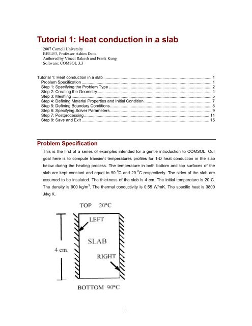
Problem Specification
This is the first of a series of examples intended for a gentle introduction to COMSOL. Our
goal here is to compute transient temperatures profiles for 1-D heat conduction in the slab
below during the heating process. The temperature in both bottom and top surfaces of the
slab are kept constant and equal to 90 0 C and 20 0 C respectively. The sides of the slab are
assumed to be insulated. The thickness of the slab is 4 cm. The initial temperature is 20 C.
The density is 900 kg/m 3 . The thermal conductivity is 0.55 W/mK. The specific heat is 3800
J/kg K.
1

Step 1: Specifying the Problem Type
The problem in this case is transient heat conduction in a 1D setting. We will first set
COMSOL up for this type of problem
The model you specify determine the Governing Equations that will be used. Starting from the
energy transport equation:
2
∂T
∂T
k ∂ T Q
+ u = +
2
{ ∂t
{ ∂x
ρc
p
∂x
ρc
p
14243
{
transient
convection
diffusion
source
(1)
For our problem, the temperatures are dependant on time; there is no fluid flow and no source
terms. The only mode of heat transfer is by diffusion. So the problem is a transient diffusion
problem with no convection and heat source. So the governing equation changes to:
∂T
∂t
=
k
ρc
p
2
∂ T
2
∂x
(2)
2

1. Start COMSOL by double
clicking on the COMSOL
Multiphysics icon on the
Desktop
2. Select 2D next to Space
Dimension
(Note: COMSOL can do 1D
problems, however to give
you a better understanding of
COMSOL we’ll model the
problem as 2D)
3. Single Click on COMSOL
Multiphysics >> Heat Transfer
>> Conduction >> Transient
Analysis. Transient Analysis
under conduction is selected
as we intend to solve a time
dependent conduction
problem (Equation 2).
4. Click on the Settings Tab
5. Set the Unit system to SI
6. Click OK. COMSOL Window
opens up.
7. Under File, click on Save
as…
8. Create your own folder using
your NetID in the My
Documents folder and save
your work there. Specify the
file name (e.g. cond.mph) and
save it as .mph file.
3

Step 2: Creating the Geometry
The geometry in this case is a 1D slab that is 4 cm high (along y axis). We are modeling the
problem as 2D and so we assume the dimension of 2 cm in the other direction (i.e. along x
axis). In this example (in contrast with the drug delivery example) we will draw out the slab
directly without specifying the grid.
1. Click on Draw >> Specify Objects >>
Rectangle. Rectangle window opens
up.
2. Specify width as 0.02 and height as
0.04. These are the dimensions of
the slab in m.
3. Click on OK.
4. Click on Zoom Extents to fit the
geometry in the window.
The geometry that is created is shown in
the figure.
4

Step 3: Meshing
Meshing is dividing the geometry into small elements. We can mesh the face directly, but in
this case, we will mesh the edges first and then the face. This method is used to control the
number of elements in certain parts of the geometry like the boundaries and interfaces. In
many cases we need a finer mesh near the boundary and so we mesh the edge accordingly
and what we get is a non-uniform mesh. However in this case we mesh the geometry with a
uniform mesh with a spacing of 0.002 between the nodes.
1. Under Mesh, click on Mapped
Mesh Parameters…
2. Click on the Boundary Tab
3. In Boundary Selection, select 1
and 4 by left clicking and holding
the Ctrl key. We will specify 20
elements each on the left and
right edges.
4. Check the box for Constrained
edge element distribution
5. Click on Number of edge
elements, and type in 20 in the
box below.
6. For boundary 2 and 3, use
number of edge elements as 10.
We specify 10 elements each on
the top and bottom edges.
7. Press the ‘Remesh’ Button on the
bottom. The mesh that is
obtained is shown in the figure.
8. Click ‘Ok’
5

9. Your screen should now look like
this.
6

Step 4: Defining Material Properties and Initial Condition
We are solving the energy equation and so we need to provide the solver with the appropriate
material property values required for the analysis. These properties are:
(i) Density (ρ): The density of the material of the slab is 900 kgm -3
(ii) Thermal Conductivity (k): The thermal conductivity is 0.55 W(mK) -1
(iii) Specific Heat (c p ): The specific heat is 3800 J (kgK) -1
The Slab is initially at a temperature of 20 0 C initially. We will also specify this in the software in
this step.
1. Under Physics, click on
Subdomain Settings…
1
2. Click on 1 to select the slab.
3. Left click on the text field next
to Thermal Conductivity and
type 0.55
4. Left click on the text field next
to Density and type 900
5. Left click on the text field next
to Heat Capacity and type 3800
6. Click on the Init Tab
7. In the box under Initial Value, fill
in 293. The slab is initially at a
temperature of 20 0 C (=293 K).
8. Click Ok
7

Step 5: Defining Boundary Conditions
The boundary conditions for the problem are:
On the bottom boundary: Temperature = 90 0 C
On the top boundary: Temperature = 20 0 C
On the left boundary: The left boundary is insulated. Therefore, Heat Flux =0.
On the right boundary: The right boundary is insulated. Therefore, Heat Flux =0.
We now specify these boundary conditions to the solver.
The default boundary condition for this solver is thermal insulation so we simply need to change
the boundary conditions for the top and bottom
1. Under Physics, click on
Boundary Settings…
2. Click on 2 in the Boundary
Selection box
3. Change the Boundary
Condition to Temperature
4. In T 0 , change the
temperature to 90. The
bottom of the slab is at
90 0 C (=363 K).
5. Repeat for side 3 using
293. The top of the slab is
at 20 0 C (=293 K).
6. Click on OK
8

Step 6: Specifying Solver Parameters
We now specify the time integration method for the time dependant problem. We use the
default values for solver settings for this problem as well. To select fixed time steps, we need
to go the “Time Stepping” Tab in the Solver Parameters window. However, we do not do this
for the problem. Variable time stepping is used as the default for this problem.
1. Under Solve, click on
Solver Parameters.
2. Under the General Tab,
select Transient under
Analysis if it is not
already selected
3. Select Time dependent
under Solver.
4. In the Times: box, type
in 0:10:5400. This tells
the solver to start at 0
seconds, then save the
solution every 10
seconds until it reaches
5400 seconds.
5. Click Ok
6. Click on Get Initial Value
under Solve. This step
initializes the solver with
the value provided when
the initial conditions
were specified (Step 4).
7. Under Solve, click on
Solver Manager.
9

8. Click on the Solve For
tab.
9. Select T for temperature
if it is not already
selected. By selecting T,
we are directing the
solver to solve for the
temperature.
10. Click on the Output tab.
11. Select T for temperature
if it is not already
selected. By selecting T,
we are directing the
program to save the
temperature values.
12. Press Solve. Once
Solve is pressed, the
solver solves the
transient heat transfer
equation (Equation 2 on
page 2). It will take
approximately 1-2 min
to solve. We are now
ready to do post
processing (looking at
the results).
10

Step 7: Postprocessing
Post-processing is viewing the results obtained on running the simulations of the problem. We
will generate graphs and charts based upon our simulation.
Displaying the Mesh
1. To display the mesh, simply click on
the Mesh Mode button. Mesh mode
can also be selected by clicking on
Mesh >> Mesh Mode.
1.
The mesh is shown in the figure below.
11

Plot Temperature vs. Time at a particular coordinate
We will now plot the temperature history at point (0.01, 0.01) in the interior of the slab to see
how the temperature varies with time at that location.
1. Under Postprocessing, click on
Cross-Section Plot Parameters… (It
may take some time to open up).
2. Click on the Point tab,
1
3. Make sure Temperature is selected in
the Predefined quantities section.
4. In Coordinates, type in 0.01 for x and
0.01 for y.
5. Press OK
The temperature history plot obtained for
the point (0.01, 0.01) is shown in the
figure below.
12

Obtain the surface plot at the last time step
We now plot the temperature contour in the slab at the end time (i.e. after 1.5 hrs or 5400 s).
1. Under Postprocessing
click on Plot Parameters.
1
2. Click on the General Tab
3. Check the box for Surface
under Plot Type.
4. Next to Solution at time:
select 5400.
5. Click on the Surface Tab.
6. Select Temperature next
to Predefined quantities, if
it is not already selected.
7. Click on OK.
The contour plot that is
obtained is shown on the next
page.
14

Step 8: Save and Exit
Now, before we end the session we need to save the files for future use.
1. Go to File
2. Click on Save
3. Go to File >> Exit
15