MAT 167: Statistics Final Exam Instructor: Anthony Tanbakuchi ...
MAT 167: Statistics Final Exam Instructor: Anthony Tanbakuchi ...
MAT 167: Statistics Final Exam Instructor: Anthony Tanbakuchi ...

You also want an ePaper? Increase the reach of your titles
YUMPU automatically turns print PDFs into web optimized ePapers that Google loves.
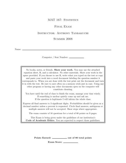
<strong>MAT</strong> <strong>167</strong>: <strong>Statistics</strong><br />
<strong>Final</strong> <strong>Exam</strong><br />
<strong>Instructor</strong>: <strong>Anthony</strong> <strong>Tanbakuchi</strong><br />
Summer 2008<br />
Name:<br />
Computer / Seat Number:<br />
No books, notes, or friends. Show your work. You may use the attached<br />
equation sheet, R, and a calculator. No other materials. Show your work in the<br />
space provided. If you choose to use R, write what you typed on the test or copy<br />
and paste your work into a word document labeling the question number it<br />
corresponds to. When you are done with the test print out the document and turn<br />
it in with the test. Be sure to save often on a memory stick just in case. Using any<br />
other program or having any other documents open on the computer will<br />
constitute cheating.<br />
You have until the end of class to finish the exam, manage your time wisely.<br />
If something is unclear quietly come up and ask me.<br />
If the question is legitimate I will inform the whole class.<br />
Express all final answers to 3 significant digits. Probabilities should be given as a<br />
decimal number unless a percent is requested. Circle final answers, ambiguous or<br />
multiple answers will not be accepted. Show steps where appropriate.<br />
The exam consists of 16 questions for a total of 80 points on 9 pages.<br />
This <strong>Exam</strong> is being given under the guidelines of our institution’s<br />
Code of Academic Ethics. You are expected to respect those guidelines.<br />
Points Earned:<br />
<strong>Exam</strong> Score:<br />
out of 80 total points
<strong>MAT</strong> <strong>167</strong>: <strong>Statistics</strong>, <strong>Final</strong> <strong>Exam</strong> p. 1 of 9<br />
1. The following is a partial list of statistical methods that we have discussed:<br />
1. mean<br />
2. median<br />
3. mode<br />
4. standard deviation<br />
5. z-score<br />
6. percentile<br />
7. coefficient of variation<br />
8. scatter plot<br />
9. histogram<br />
10. pareto chart<br />
11. box plot<br />
12. normal-quantile plot<br />
13. confidence interval for a mean<br />
14. confidence interval for difference in means<br />
15. confidence interval for a proportion<br />
16. confidence interval for difference in proportions<br />
17. one sample mean test<br />
18. two independent sample mean test<br />
19. one sample proportion test<br />
20. two sample proportion test<br />
21. test of homogeneity<br />
22. test of independence<br />
23. linear correlation coefficient & test<br />
24. regression<br />
25. 1-way ANOVA<br />
For each situation below, which method is most applicable?<br />
• If it’s a hypothesis test, also state what the null and alternative hypothesis are.<br />
• If it’s a graphical method, also describe what you would be looking for.<br />
• If it’s a statistic, how susceptible to outliers is it?<br />
(a) (2 points) A researcher at the department of labor wants to determine if the proportion of<br />
men who work in sociology, psychology, and anthropology is the same from recent study<br />
data on the subject.<br />
(b) (2 points) A math department committee wants to award $50 to the student who received<br />
the best score on their calculus final exam this past semester. However, the three faculty<br />
who taught calculus last semester gave different final exams. What method could help<br />
identify the top student amongst the three different exams?<br />
(c) (2 points) A drug research would like to test the claim that the mean absorption of 1 gram<br />
of vitamin E is the same for four methods of delivery: topical, intravenous, oral, and nasal<br />
<strong>Instructor</strong>: <strong>Anthony</strong> <strong>Tanbakuchi</strong> Points earned: / 6 points
<strong>MAT</strong> <strong>167</strong>: <strong>Statistics</strong>, <strong>Final</strong> <strong>Exam</strong> p. 2 of 9<br />
spray.<br />
(d) (2 points) A researcher is using a statistical hypothesis test that requires the population<br />
which the sample was drawn from to have a normal distribution. How could the researcher<br />
check this assumption?<br />
(e) (2 points) A drug researcher wants to determine if a new growth hormone drug can increase<br />
the mean weight of mice as compared to a control group of mice.<br />
2. (1 point) The test of homogeneity can be thought of as a generalization of what two sample<br />
test?<br />
3. (1 point) If the mean, median, and mode for a data set are all the same, what can you conclude<br />
about the data’s distribution?<br />
4. (2 points) Under what conditions can we approximate a binomial distribution as a normal<br />
distribution?<br />
5. (2 points) Give a clear specific example of when you would use a population distribution.<br />
<strong>Instructor</strong>: <strong>Anthony</strong> <strong>Tanbakuchi</strong> Points earned: / 10 points
<strong>MAT</strong> <strong>167</strong>: <strong>Statistics</strong>, <strong>Final</strong> <strong>Exam</strong> p. 3 of 9<br />
6. (2 points) Give a clear specific example example of when you would use a sampling distribution.<br />
7. (1 point) What percent of data lies within one standard deviation as stated by the Empirical<br />
Rule?<br />
8. The following questions regard hypothesis testing in general.<br />
(a) (1 point) When we conduct a hypothesis test, we assume something is true and calculate<br />
the probability of observing the sample data under this assumption. What do we assume<br />
is true?<br />
(b) (1 point) Do we use the population distribution or the sampling distribution when calculating<br />
the p-value?<br />
(c) (1 point) If you fail to reject H 0 but H 0 is false. What type of error has occurred? (Type<br />
I or Type II)<br />
(d) (1 point) What variable represents the actual Type I error?<br />
(e) (1 point) What variable is used to represent a Type II error?<br />
(f) (1 point) What does the power of a hypothesis test represent?<br />
(g) (1 point) In the one sample mean test with σ unknown, what is the distribution of the<br />
test statistic?<br />
(h) (2 points) Why is it important to use random sampling?<br />
9. A consumer advocate group believes that Crystal Springs Sparkling Mineral Water contains<br />
more than the advertised 35 mg of sodium per serving. They randomly sample 40 servings<br />
<strong>Instructor</strong>: <strong>Anthony</strong> <strong>Tanbakuchi</strong> Points earned: / 12 points
<strong>MAT</strong> <strong>167</strong>: <strong>Statistics</strong>, <strong>Final</strong> <strong>Exam</strong> p. 4 of 9<br />
and measure the amount of sodium contained in each sample. The collected data has a sample<br />
mean of 37.5 mg, and a sample standard deviation of 8.2 mg.<br />
(a) (2 points) What is the null and alternative hypothesis?<br />
(b) (1 point) What hypothesis test should be used?<br />
(c) (2 points) What are the requirements for the hypothesis test? Are they met?<br />
(d) (1 point) What significance level will you use?<br />
(e) (2 points) Manually compute the p-value.<br />
(f) (1 point) What is the formal decision?<br />
(g) (2 points) What is the final conclusion?<br />
10. A craps table at a local casino has been losing more money than normal. It seems that bets<br />
involving a one on the face of the dice (such as “snake eyes”) are appearing more than usual.<br />
The casino manager thinks that the dice have been weighted to cause the side with one to have<br />
a higher probability of occurring than a fair dice.<br />
(a) (2 points) The casino manager takes one of the dice from the table and flips it 100 times,<br />
the side with a value of one appears 26 times. Construct a 95% confidence interval for the<br />
<strong>Instructor</strong>: <strong>Anthony</strong> <strong>Tanbakuchi</strong> Points earned: / 13 points
<strong>MAT</strong> <strong>167</strong>: <strong>Statistics</strong>, <strong>Final</strong> <strong>Exam</strong> p. 5 of 9<br />
true probability of getting a one with this die.<br />
(b) (1 point) If the die is fair, what should the true probability be for getting a one?<br />
(c) (1 point) Why can’t the casino manager conclude that the die is unfair simply based on<br />
the fact that he observed one appear more than it theoretically should have appeared?<br />
What other explanation could account for this?<br />
(d) (1 point) Now the casino manager would like to conduct a hypothesis test to determine if<br />
the die is unfair. What type of hypothesis test should he use?<br />
(e) (2 points) What are the manager’s hypothesis for the test?<br />
(f) (2 points) What are the test’s requirements? Are they satisfied?<br />
<strong>Instructor</strong>: <strong>Anthony</strong> <strong>Tanbakuchi</strong> Points earned: / 7 points
<strong>MAT</strong> <strong>167</strong>: <strong>Statistics</strong>, <strong>Final</strong> <strong>Exam</strong> p. 6 of 9<br />
(g) (2 points) Conduct the hypothesis test, what is the p-value?<br />
(h) (1 point) What is the formal decision?<br />
(i) (1 point) What is the conclusion?<br />
(j) (1 point) What is the probability of a Type I error for this study?<br />
11. Eighteen students were randomly selected to take the SAT after having either no breakfast or<br />
a complete breakfast A researcher would like to test the claim that students who eat breakfast<br />
score higher than students who do not.<br />
Group without breakfast: SAT Score 480 510 530 540 550 560 600 620 660<br />
Group with breakfast: SAT Score 460 500 530 520 580 580 560 640 690<br />
(a) (1 point) What type of hypothesis test will you use?<br />
(b) (2 points) What are the test’s requirements?<br />
(c) (2 points) What are the hypothesis H 0 and H a ?<br />
(d) (1 point) What α will you use?<br />
(e) (2 points) Conduct the hypothesis test. What is the p-value?<br />
(f) (1 point) What is your formal decision?<br />
<strong>Instructor</strong>: <strong>Anthony</strong> <strong>Tanbakuchi</strong> Points earned: / 14 points
<strong>MAT</strong> <strong>167</strong>: <strong>Statistics</strong>, <strong>Final</strong> <strong>Exam</strong> p. 7 of 9<br />
(g) (2 points) State your final conclusion in words.<br />
12. The following table lists the the fuel consumption (in miles/gallon) and weight (in lbs) of a<br />
vehicle.<br />
Weight 3180 3450 3225 3985 2440 2500 2290<br />
MPG 27 29 27 24 37 34 37<br />
(a) (2 points) Upon looking at the scatter plot of the data, the relationship of fuel consumption<br />
and milage looks linear. Is the linear relationship statistically significant? (Justify your<br />
answer with an analysis.)<br />
(b) (1 point) What percent of a vehicle’s fuel consumption can be explained by its weight?<br />
(c) (2 points) You are designing a new vehicle and would like to be able to predict its fuel<br />
consumption. Write the equation for fitted model (with the actual values of the coefficients).<br />
(d) (1 point) What range of vehicle weights is the model valid for making predictions of fuel<br />
efficiency?<br />
(e) (1 point) What is the best predicted fuel consumption for a new vehicle that weights 3200<br />
lbs?<br />
(f) (1 point) If the liner relationship had not been statistically significant, what is the best<br />
predicted fuel consumption for a new vehicle that weights 3200 lbs?<br />
<strong>Instructor</strong>: <strong>Anthony</strong> <strong>Tanbakuchi</strong> Points earned: / 10 points
<strong>MAT</strong> <strong>167</strong>: <strong>Statistics</strong>, <strong>Final</strong> <strong>Exam</strong> p. 8 of 9<br />
13. (2 points) A random sample of 5 chihuahuas was conducted to determine the mean tong length<br />
of the breed. Below is the study data in inches.<br />
1.6, 2.1, 1.5, 1.9, 2<br />
Construct a 90% confidence interval for the true population mean using the above data.<br />
(Assume σ is unknown.)<br />
14. (2 points) A ski resort is designing a new super tram to carry 40 people. If the mean weight of<br />
humans is approximately 165 lbs with a standard deviation of 25 lbs, what should the tram’s<br />
maximum weight limit be so that it can carry the desired capacity 95% of the time?<br />
<strong>Instructor</strong>: <strong>Anthony</strong> <strong>Tanbakuchi</strong> Points earned: / 4 points
<strong>MAT</strong> <strong>167</strong>: <strong>Statistics</strong>, <strong>Final</strong> <strong>Exam</strong> p. 9 of 9<br />
15. (2 points) You would like to conduct a study to estimate (at the 90% confidence level) the<br />
mean weight of brown bears with a margin of error of 5 lbs. A preliminary study indicates that<br />
bear weights are normally distributed with a standard deviation of 22 lbs, what sample size<br />
should you use for this study?<br />
16. (2 points) Given y = {a, −2a, 4a}, where a is a constant, completely simplify the following<br />
expression:<br />
(∑<br />
yi<br />
) 2<br />
− 2<br />
************<br />
End of exam. Reference sheets follow.<br />
<strong>Instructor</strong>: <strong>Anthony</strong> <strong>Tanbakuchi</strong> Points earned: / 4 points
<strong>Statistics</strong> Quick Reference<br />
Card & R Commands<br />
by <strong>Anthony</strong> <strong>Tanbakuchi</strong>. Version 1.8.2<br />
http://www.tanbakuchi.com<br />
ANTHONY@TANBAKUCHI·COM<br />
Get R at: http://www.r-project.org<br />
R commands: bold typewriter text<br />
1 Misc R<br />
To make a vector / store data: x=c(x1, x2, ...)<br />
Help: general RSiteSearch("Search Phrase")<br />
Help: function ?functionName<br />
Get column of data from table:<br />
tableName$columnName<br />
List all variables: ls()<br />
Delete all variables: rm(list=ls())<br />
√ x = sqrt(x) (1)<br />
x n = x ∧ n (2)<br />
n = length(x) (3)<br />
T = table(x) (4)<br />
2 Descriptive <strong>Statistics</strong><br />
2.1 NUMERICAL<br />
Let x=c(x1, x2, x3, ...)<br />
n<br />
total = ∑ xi = sum(x) (5)<br />
i=1<br />
min = min(x) (6)<br />
max = max(x) (7)<br />
six number summary : summary(x) (8)<br />
µ = ∑xi<br />
N<br />
¯x = ∑xi<br />
n<br />
= mean(x) (9)<br />
= mean(x) (10)<br />
˜x = P50 = median(x) (11)<br />
√<br />
∑(xi − µ) 2<br />
σ =<br />
(12)<br />
N<br />
√<br />
∑(xi − ¯x) 2<br />
s =<br />
= sd(x) (13)<br />
n − 1<br />
CV = σ µ = s¯x<br />
2.2 RELATIVE STANDING<br />
z = x − µ<br />
σ<br />
= x − ¯x<br />
s<br />
Percentiles:<br />
Pk = xi, (sorted x)<br />
(14)<br />
(15)<br />
k = i − 0.5 · 100% (16)<br />
n<br />
To find xi given Pk, i is:<br />
1. L = (k/100%)n<br />
2. if L is an integer: i = L + 0.5;<br />
otherwise i=L and round up.<br />
2.3 VISUAL<br />
All plots have optional arguments:<br />
• main="" sets title<br />
• xlab="", ylab="" sets x/y-axis label<br />
• type="p" for point plot<br />
• type="l" for line plot<br />
• type="b" for both points and lines<br />
Ex: plot(x, y, type="b", main="My Plot")<br />
Plot Types:<br />
hist(x) histogram<br />
stem(x) stem & leaf<br />
boxplot(x) box plot<br />
plot(T) bar plot, T=table(x)<br />
plot(x,y) scatter plot, x, y are ordered vectors<br />
plot(t,y) time series plot, t, y are ordered vectors<br />
curve(expr, xmin,xmax) plot expr involving x<br />
2.4 ASSESSING NORMALITY<br />
Q-Q plot: qqnorm(x); qqline(x)<br />
3 Probability<br />
Number of successes x with n possible outcomes.<br />
(Don’t double count!)<br />
P(A) = xA n<br />
(17)<br />
P(Ā) = 1 − P(A) (18)<br />
P(A or B) = P(A) + P(B) − P(A and B) (19)<br />
P(A or B) = P(A) + P(B) if A,B mut. excl. (20)<br />
P(A and B) = P(A) · P(B|A) (21)<br />
P(A and B) = P(A) · P(B) if A,B independent (22)<br />
n! = n(n − 1)···1 = factorial(n) (23)<br />
nPk = n!<br />
(n − k)!<br />
=<br />
nCk =<br />
n!<br />
n1!n2!···nk!<br />
n!<br />
(n − k)!k!<br />
4 Discrete Random Variables<br />
Perm. no elem. alike (24)<br />
Perm. n1 alike, . . . (25)<br />
= choose(n,k) (26)<br />
P(xi) : probability distribution (27)<br />
E = µ = ∑xi · P(xi) (28)<br />
√<br />
σ = ∑(xi − µ) 2 · P(xi) (29)<br />
4.1 BINOMIAL DISTRIBUTION<br />
µ = n · p (30)<br />
σ = √ n · p · q (31)<br />
P(x) = nCx p x q (n−x) = dbinom(x, n, p) (32)<br />
4.2 POISSON DISTRIBUTION<br />
P(x) = µx · e −µ<br />
= dpois(x, µ) (33)<br />
x!<br />
5 Continuous random variables<br />
CDF F(x) gives area to the left of x, F −1 (p) expects p<br />
is area to the left.<br />
f (x) : probability density (34)<br />
Z ∞<br />
E = µ = x · f (x)dx (35)<br />
−∞<br />
√Z ∞<br />
σ = (x − µ) 2 · f (x)dx (36)<br />
−∞<br />
F(x) : cumulative prob. density (CDF) (37)<br />
F −1 (x) : inv. cumulative prob. density (38)<br />
Z x<br />
F(x) = f (x ′ )dx ′ (39)<br />
−∞<br />
p = P(x < x ′ ) = F(x ′ ) (40)<br />
x ′ = F −1 (p) (41)<br />
p = P(x > a) = 1 − F(a) (42)<br />
p = P(a < x < b) = F(b) − F(a) (43)<br />
5.1 UNIFORM DISTRIBUTION<br />
p = P(u < u ′ ) = F(u ′ )<br />
= punif(u’, min=0, max=1) (44)<br />
u ′ = F −1 (p) = qunif(p, min=0, max=1) (45)<br />
5.2 NORMAL DISTRIBUTION<br />
f (x) =<br />
1<br />
√<br />
2πσ 2 · e− 1 2<br />
(x−µ) 2<br />
σ 2 (46)<br />
p = P(z < z ′ ) = F(z ′ ) = pnorm(z’) (47)<br />
z ′ = F −1 (p) = qnorm(p) (48)<br />
p = P(x < x ′ ) = F(x ′ )<br />
= pnorm(x’, mean=µ, sd=σ) (49)<br />
x ′ = F −1 (p)<br />
= qnorm(p, mean=µ, sd=σ) (50)<br />
5.3 t-DISTRIBUTION<br />
p = P(t < t ′ ) = F(t ′ ) = pt(t’, df) (51)<br />
t ′ = F −1 (p) = qt(p, df) (52)<br />
5.4 χ 2 -DISTRIBUTION<br />
p = P(χ 2 < χ 2′ ) = F(χ 2′ )<br />
= pchisq(X 2 ’, df) (53)<br />
χ 2′ = F −1 (p) = qchisq(p, df) (54)<br />
5.5 F-DISTRIBUTION<br />
p = P(F < F ′ ) = F(F ′ )<br />
= pf(F’, df1, df2) (55)<br />
F ′ = F −1 (p) = qf(p, df1, df2) (56)<br />
6 Sampling distributions<br />
µ ¯x = µ σ ¯x = σ √ n<br />
(57)<br />
µ ˆp = p σ ˆp =<br />
√ pq<br />
7 Estimation<br />
7.1 CONFIDENCE INTERVALS<br />
n<br />
(58)<br />
proportion: ˆp ± E, E = z α/2 · σ ˆp (59)<br />
mean (σ known): ¯x ± E, E = z α/2 · σ ¯x (60)<br />
mean (σ unknown, use s): ¯x ± E, E = t α/2 · σ ¯x, (61)<br />
d f = n − 1<br />
variance:<br />
(n − 1)s2<br />
χ 2 R<br />
< σ 2 <<br />
(n − 1)s2<br />
d f = n − 1<br />
√<br />
p1 ˆ q1 ˆ<br />
2 proportions: ∆ ˆp ± z α/2 ·<br />
n1<br />
√<br />
s 2 1<br />
2 means (indep): ∆ ¯x ±t α/2 ·<br />
n1<br />
d f ≈ min(n1 − 1, n2 − 1)<br />
χ 2 L<br />
+ p2 ˆ q2 ˆ<br />
n2<br />
+ s2 2<br />
n2<br />
, (62)<br />
(63)<br />
, (64)<br />
matched pairs: d ¯±t α/2 · √ sd , di = xi − yi, (65)<br />
n<br />
d f = n − 1<br />
7.2 CI CRITICAL VALUES (TWO SIDED)<br />
z α/2 = F −1<br />
z (1 − α/2) = qnorm(1-alpha/2) (66)<br />
t α/2 = F −1<br />
t (1 − α/2) = qt(1-alpha/2, df) (67)<br />
χ 2 L = F −1<br />
χ2 (α/2) = qchisq(alpha/2, df) (68)<br />
χ 2 R = F −1<br />
χ 2 (1 − α/2) = qchisq(1-alpha/2, df)<br />
7.3 REQUIRED SAMPLE SIZE<br />
(69)<br />
( zα/2<br />
)2<br />
proportion: n = ˆp ˆq , (70)<br />
E<br />
( ˆp = ˆq = 0.5 if unknown)<br />
( ) zα/2 · ˆσ 2<br />
mean: n =<br />
(71)<br />
E
8 Hypothesis Tests<br />
Test statistic and R function (when available) are listed for each.<br />
Optional arguments for hypothesis tests:<br />
alternative="two.sided" can be:<br />
"two.sided", "less", "greater"<br />
conf.level=0.95 constructs a 95% confidence interval. Standard CI<br />
only when alternative="two.sided".<br />
Optional arguments for power calculations & Type II error:<br />
alternative="two.sided" can be:<br />
"two.sided" or "one.sided"<br />
sig.level=0.05 sets the significance level α.<br />
8.1 1-SAMPLE PROPORTION<br />
H0 : p = p0<br />
prop.test(x, n, p=p0, alternative="two.sided")<br />
ˆp − p0<br />
z = √<br />
p0q0/n<br />
8.2 1-SAMPLE MEAN (σ KNOWN)<br />
H0 : µ = µ0<br />
z =<br />
¯x − µ0<br />
σ/ √ n<br />
8.3 1-SAMPLE MEAN (σ UNKNOWN)<br />
(72)<br />
(73)<br />
H0 : µ = µ0<br />
t.test(x, mu=µ0, alternative="two.sided")<br />
Where x is a vector of sample data.<br />
¯x − µ0<br />
t =<br />
s/ √ n , d f = n − 1 (74)<br />
Required Sample size:<br />
power.t.test(delta=h, sd =σ, sig.level=α, power=1 −<br />
β, type ="one.sample", alternative="two.sided")<br />
8.4 2-SAMPLE PROPORTION TEST<br />
H0 : p1 = p2 or equivalently H0 : ∆p = 0<br />
prop.test(x, n, alternative="two.sided")<br />
where: x=c(x1, x2) and n=c(n1, n2)<br />
∆ ˆp − ∆p0<br />
z = √ , ∆ ˆp = ˆp1 − ˆp2 (75)<br />
¯p ¯q ¯p ¯q<br />
+ n1 n2<br />
x1 + x2<br />
¯p = , ¯q = 1 − ¯p (76)<br />
n1 + n2<br />
Required Sample size:<br />
power.prop.test(p1=p1, p2=p2, power=1 − β,<br />
sig.level=α, alternative="two.sided")<br />
8.5 2-SAMPLE MEAN TEST<br />
H0 : µ1 = µ2 or equivalently H0 : ∆µ = 0<br />
t.test(x1, x2, alternative="two.sided")<br />
where: x1 and x2 are vectors of sample 1 and sample 2 data.<br />
∆ ¯x − ∆µ0<br />
t = √ d f ≈ min(n1 − 1, n2 − 1), ∆ ¯x = ¯x1 − ¯x2 (77)<br />
s 2 1 + s2 2<br />
n1 n2<br />
Required Sample size:<br />
power.t.test(delta=h, sd =σ, sig.level=α, power=1<br />
β, type ="two.sample", alternative="two.sided")<br />
−<br />
8.6 2-SAMPLE <strong>MAT</strong>CHED PAIRS TEST<br />
H0 : µd = 0<br />
t.test(x, y, paired=TRUE, alternative="two.sided")<br />
where: x and y are ordered vectors of sample 1 and sample 2 data.<br />
t = d¯<br />
− µd0<br />
sd/ √ n<br />
, di = xi − yi, d f = n − 1 (78)<br />
Required Sample size:<br />
power.t.test(delta=h, sd =σ, sig.level=α, power=1<br />
β, type ="paired", alternative="two.sided")<br />
8.7 TEST OF HOMOGENEITY, TEST OF INDEPENDENCE<br />
H0 : p1 = p2 = ··· = pn (homogeneity)<br />
H0 : X and Y are independent (independence)<br />
chisq.test(D)<br />
Enter table: D=data.frame(c1, c2, ...), where c1, c2, ... are<br />
column data vectors.<br />
Or generate table: D=table(x1, x2), where x1, x2 are ordered vectors<br />
of raw categorical data.<br />
χ 2 (Oi − Ei)2<br />
= ∑ , d f = (num rows - 1)(num cols - 1) (79)<br />
Ei<br />
(row total)(column total)<br />
Ei = = npi (80)<br />
(grand total)<br />
For 2 × 2 contingency tables, you can use the Fisher Exact Test:<br />
fisher.test(D, alternative="greater")<br />
(must specify alternative as greater)<br />
9 Linear Regression<br />
9.1 LINEAR CORRELATION<br />
H0 : ρ = 0<br />
cor.test(x, y)<br />
where: x and y are ordered vectors.<br />
r =<br />
∑(xi − ¯x)(yi − ȳ)<br />
(n − 1)sxsy<br />
, t = √<br />
r − 0<br />
1−r 2<br />
n−2<br />
−<br />
, d f = n − 2 (81)<br />
9.2 MODELS IN R<br />
MODEL TYPE EQUATION R MODEL<br />
linear 1 indep var y = b0 + b1x1 y∼x1<br />
. . . 0 intercept y = 0 + b1x1 y∼0+x1<br />
linear 2 indep vars y = b0 + b1x1 + b2x2 y∼x1+x2<br />
. . . inteaction y = b0 + b1x1 + b2x2 + b12x1x2 y∼x1+x2+x1*x2<br />
polynomial y = b0 + b1x1 + b2x2 2 y∼x1+I(x2 ∧ 2)<br />
9.3 REGRESSION<br />
Simple linear regression steps:<br />
1. Make sure there is a significant linear correlation.<br />
2. results=lm(y∼x) Linear regression of y on x vectors<br />
3. results View the results<br />
4. plot(x, y); abline(results) Plot regression line on data<br />
5. plot(x, results$residuals) Plot residuals<br />
y = b0 + b1x1 (82)<br />
b1 =<br />
∑(xi − ¯x)(yi − ȳ)<br />
∑(xi − ¯x) 2 (83)<br />
b0 = ȳ − b1 ¯x (84)<br />
9.4 PREDICTION INTERVALS<br />
To predict y when x = 5 and show the 95% prediction interval with regression<br />
model in results:<br />
predict(results, newdata=data.frame(x=5),<br />
int="pred")<br />
10 ANOVA<br />
10.1 ONE WAY ANOVA<br />
1. results=aov(depVarColName∼indepVarColName,<br />
data=tableName) Run ANOVA with data in TableName,<br />
factor data in indepVarColName column, and response data in<br />
depVarColName column.<br />
2. summary(results) Summarize results<br />
3. boxplot(depVarColName∼indepVarColName,<br />
data=tableName) Boxplot of levels for factor<br />
F = MS(treatment)<br />
MS(error)<br />
, d f1 = k − 1, d f2 = N − k (85)<br />
To find required sample size and power see power.anova.test(...)<br />
11 Loading and using external data and tables<br />
11.1 LOADING EXCEL DATA<br />
1. Export your table as a CSV file (comma seperated file) from Excel.<br />
2. Import your table into MyTable in R using:<br />
MyTable=read.csv(file.choose())<br />
11.2 LOADING AN .RDATA FILE<br />
You can either double click on the .RData file or use the menu:<br />
• Windows: File→Load Workspace. . .<br />
• Mac: Workspace→Load Workspace File. . .<br />
11.3 USING TABLES OF DATA<br />
1. To see all the available variables type: ls()<br />
2. To see what’s inside a variable, type its name.<br />
3. If the variable tableName is a table, you can also type<br />
names(tableName) to see the column names or type<br />
head(tableName) to see the first few rows of data.<br />
4. To access a column of data type tableName$columnName<br />
An example demonstrating how to get the women’s height data and find the<br />
mean:<br />
> ls() # See what variables are defined<br />
[1] "women" "x"<br />
> head(women) #Look at the first few entries<br />
height weight<br />
1 58 115<br />
2 59 117<br />
3 60 120<br />
> names(women) # Just get the column names<br />
[1] "height" "weight"<br />
> women$height # Display the height data<br />
[1] 58 59 60 61 62 63 64 65 66 67 68 69 70 71 72<br />
> mean(women$height) # Find the mean of the heights<br />
[1] 65