MAT 167: Statistics Midterm Exam Instructor: Anthony Tanbakuchi ...
MAT 167: Statistics Midterm Exam Instructor: Anthony Tanbakuchi ...
MAT 167: Statistics Midterm Exam Instructor: Anthony Tanbakuchi ...

You also want an ePaper? Increase the reach of your titles
YUMPU automatically turns print PDFs into web optimized ePapers that Google loves.
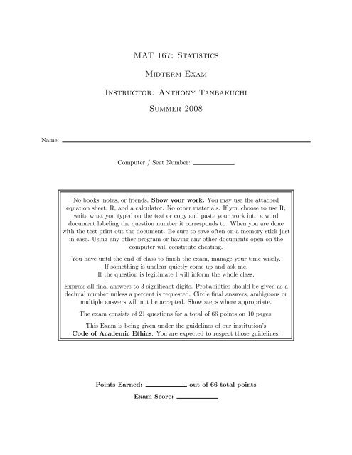
<strong>MAT</strong> <strong>167</strong>: <strong>Statistics</strong><br />
<strong>Midterm</strong> <strong>Exam</strong><br />
<strong>Instructor</strong>: <strong>Anthony</strong> <strong>Tanbakuchi</strong><br />
Summer 2008<br />
Name:<br />
Computer / Seat Number:<br />
No books, notes, or friends. Show your work. You may use the attached<br />
equation sheet, R, and a calculator. No other materials. If you choose to use R,<br />
write what you typed on the test or copy and paste your work into a word<br />
document labeling the question number it corresponds to. When you are done<br />
with the test print out the document. Be sure to save often on a memory stick just<br />
in case. Using any other program or having any other documents open on the<br />
computer will constitute cheating.<br />
You have until the end of class to finish the exam, manage your time wisely.<br />
If something is unclear quietly come up and ask me.<br />
If the question is legitimate I will inform the whole class.<br />
Express all final answers to 3 significant digits. Probabilities should be given as a<br />
decimal number unless a percent is requested. Circle final answers, ambiguous or<br />
multiple answers will not be accepted. Show steps where appropriate.<br />
The exam consists of 21 questions for a total of 66 points on 10 pages.<br />
This <strong>Exam</strong> is being given under the guidelines of our institution’s<br />
Code of Academic Ethics. You are expected to respect those guidelines.<br />
Points Earned:<br />
<strong>Exam</strong> Score:<br />
out of 66 total points
<strong>MAT</strong> <strong>167</strong>: <strong>Statistics</strong>, <strong>Midterm</strong> <strong>Exam</strong> p. 1 of 10<br />
1. The following is a partial list of statistical methods that we have discussed:<br />
1. mean<br />
2. median<br />
3. mode<br />
4. standard deviation<br />
5. z-score<br />
6. percentile<br />
7. coefficient of variation<br />
8. scatter plot<br />
9. histogram<br />
10. pareto chart<br />
11. box plot<br />
12. normal-quantile plot<br />
13. confidence interval for a mean<br />
14. confidence interval for a proportion<br />
For each situation below, which method is most applicable To get full points, give a short<br />
(1-3 sentence) description as to why your chosen method is appropriate!<br />
• If it’s a graphical method, also describe what you would be looking for.<br />
• If it’s a statistic, how susceptible to outliers is it<br />
(a) (2 points) A school board thinks that students might do better in morning math classes.<br />
They would like to compare the distribution of student math scores for 4 time categories:<br />
early morning classes, mid morning classes, early afternoon classes, and late afternoon<br />
classes.<br />
(b) (2 points) A clothing manufacturer wants to determine how much variability there is in<br />
toddler waist sizes.<br />
(c) (2 points) The Tucson realtors association is publishing their semi-annual newsletter and<br />
has an article discussing current housing prices. They would like to publish a single number<br />
<strong>Instructor</strong>: <strong>Anthony</strong> <strong>Tanbakuchi</strong> Points earned: / 6 points
<strong>MAT</strong> <strong>167</strong>: <strong>Statistics</strong>, <strong>Midterm</strong> <strong>Exam</strong> p. 2 of 10<br />
that is representative of the typical house price in Tucson.<br />
(d) (2 points) A political science researcher at the U of A wants to estimate the true percentage<br />
of Tucson residents who support Obama from a random survey of 1,000 people.<br />
2. (1 point) Make a sketch of a normal distribution that has been positively skewed.<br />
3. (1 point) What is the area under a positively skewed normal distribution<br />
4. (1 point) If the mean, median, and mode for a data set are not the same, what can you conclude<br />
about the data’s distribution<br />
<strong>Instructor</strong>: <strong>Anthony</strong> <strong>Tanbakuchi</strong> Points earned: / 5 points
<strong>MAT</strong> <strong>167</strong>: <strong>Statistics</strong>, <strong>Midterm</strong> <strong>Exam</strong> p. 3 of 10<br />
5. (2 points) Give an example of sampling error.<br />
6. In regards to ¯x and the Central Limit Theorem:<br />
(a) (2 points) What are the two conditions under which the CLT applies<br />
(b) (2 points) If the conditions are met, what type of distribution will ¯x have<br />
7. (2 points) Under what conditions can we approximate a binomial distribution as a normal<br />
distribution<br />
8. (2 points) Which distribution (normal, binomial, both, or neither) would be appropriate for<br />
describing:<br />
The sampling distribution of the mean for a random sample from a uniformly distributed<br />
population using a sample size of 10.<br />
9. (2 points) Give a clear specific example of when you would use a population distribution.<br />
10. (2 points) Give an example of when you would use a sampling distribution.<br />
<strong>Instructor</strong>: <strong>Anthony</strong> <strong>Tanbakuchi</strong> Points earned: / 14 points
<strong>MAT</strong> <strong>167</strong>: <strong>Statistics</strong>, <strong>Midterm</strong> <strong>Exam</strong> p. 4 of 10<br />
11. Super Fruity Chew candy has a mean weight of 500 g and a standard deviation of 10 g.<br />
(a) (2 points) Construct an interval using the Empirical Rule which you would expect 95% of<br />
the weights to fall within.<br />
(b) (2 points) Would you consider a candy with weight of 468 g unusual (State why.)<br />
12. Given the following frequency table summarizing data from a study:<br />
age.years frequency<br />
0-9 5.00<br />
10-19 8.00<br />
20-29 12.00<br />
30-39 2.00<br />
(a) (2 points) Construct a relative frequency table.<br />
(b) (1 point) What is the probability of randomly selecting someone from the study who is<br />
between 20-39 years old<br />
<strong>Instructor</strong>: <strong>Anthony</strong> <strong>Tanbakuchi</strong> Points earned: / 7 points
<strong>MAT</strong> <strong>167</strong>: <strong>Statistics</strong>, <strong>Midterm</strong> <strong>Exam</strong> p. 5 of 10<br />
(c) (2 points) Calculate the approximate mean age of the subjects in the study from the data<br />
given.<br />
13. Results from a randomized experiment to compare crop yields (as measured by dried weight<br />
of plants in grams) obtained under a control and two different treatment conditions are shown<br />
with a box plot of the data. The researcher who has developed the two new treatments hopes<br />
that at least one increases crop yield as compared to the control group.<br />
●<br />
yield weight<br />
3.5 4.5 5.5<br />
ctrl trt1 trt2<br />
treatment<br />
(a) (1 point) Did any groups contain an outlier If so which ones<br />
(b) (1 point) What group had the least variability<br />
(c) (1 point) What was the approximate IQR for the control group (ctrl)<br />
(d) (1 point) Which group had the highest median crop yield What was the median value<br />
<strong>Instructor</strong>: <strong>Anthony</strong> <strong>Tanbakuchi</strong> Points earned: / 6 points
<strong>MAT</strong> <strong>167</strong>: <strong>Statistics</strong>, <strong>Midterm</strong> <strong>Exam</strong> p. 6 of 10<br />
14. (2 points) You would like to conduct a study to estimate (at the 90% confidence level) the<br />
mean weight of brown bears with a margin of error of 5 lbs. A preliminary study indicates that<br />
bear weights are normally distributed with a standard deviation of 22 lbs, what sample size<br />
should you use for this study<br />
15. (2 points) A random sample of 5 men was conducted to determine the mean resting heart rate.<br />
Below is the study data in beats per minute.<br />
68.9, 71.9, 61.2, 77.9, 74.2<br />
Construct a 99% confidence interval for the true population mean resting heart rate for men<br />
using the above data. (Assume σ is unknown and the population is normally distributed.)<br />
16. A bag of M&M’s contains 18 red, 12 blue, 8 green, and 7 brown candies.<br />
(a) (2 points) What is the probability of randomly selecting a red or brown M&M<br />
<strong>Instructor</strong>: <strong>Anthony</strong> <strong>Tanbakuchi</strong> Points earned: / 6 points
<strong>MAT</strong> <strong>167</strong>: <strong>Statistics</strong>, <strong>Midterm</strong> <strong>Exam</strong> p. 7 of 10<br />
(b) (2 points) If 8 M&M’s are randomly selected with replacement, what is the probability of<br />
getting exactly 6 red M&M’s<br />
(c) (1 point) Would it be unusual to observe 6 red out of 8 randomly selected M&M’s (Why)<br />
17. Answer the following question for a couple who had 4 children.<br />
(a) (1 point) Is the probability of a girl considered independent or dependent for each successive<br />
birth<br />
(b) (2 points) What is the probability that the couple has at least 1 girl<br />
(c) (2 points) What is the probability that all 4 children are born on different days of the<br />
year<br />
<strong>Instructor</strong>: <strong>Anthony</strong> <strong>Tanbakuchi</strong> Points earned: / 8 points
<strong>MAT</strong> <strong>167</strong>: <strong>Statistics</strong>, <strong>Midterm</strong> <strong>Exam</strong> p. 8 of 10<br />
18. (2 points) With one method of a procedure called acceptance sampling, a sample of items is<br />
randomly selected without replacement and the entire batch is accepted if every item in the<br />
sample is okay. The Niko Electronics Company has just manufactured 10,000 CDs, and 500<br />
are defective. If 10 of the CDs are randomly selected for testing without replacement, what is<br />
the probability that the entire batch will be accepted<br />
19. Engineers must consider the breadths of male heads when designing motorcycle helmets. Men<br />
have head breadths that are normally distributed with a mean of 6.0 in and a standard deviation<br />
of 1.0 in (based on anthropometric survey data from Gordon, Churchill, et al.).<br />
(a) (2 points) If 1 man is randomly selected, find the probability that his head breadth is<br />
between 6.1 and 6.6 inches.<br />
(b) (2 points) If 1 man is randomly selected, find the probability that his head breadth is less<br />
than 6.1 in.<br />
(c) (2 points) If 30 men are randomly selected, find the probability that their mean head<br />
<strong>Instructor</strong>: <strong>Anthony</strong> <strong>Tanbakuchi</strong> Points earned: / 8 points
<strong>MAT</strong> <strong>167</strong>: <strong>Statistics</strong>, <strong>Midterm</strong> <strong>Exam</strong> p. 9 of 10<br />
breadth is less than 6.1 in.<br />
20. A craps table at a local casino has been losing more money than normal. It seems that bets<br />
involving a one on the face of the dice (such as “snake eyes”) are appearing more than usual.<br />
The casino manager thinks that the dice have been weighted to cause the side with one to have<br />
a higher probability of occurring than a fair dice.<br />
(a) (2 points) The casino manager takes one of the dice from the table and flips it 100 times,<br />
the side with a value of one appears 22 times. Construct a 95% confidence interval for the<br />
true probability of getting a one with this die.<br />
(b) (1 point) If the die is fair, what should the true probability be for getting a one<br />
(c) (1 point) Based on the casino manager’s experiment, does the die appear to be unfair<br />
Why<br />
<strong>Instructor</strong>: <strong>Anthony</strong> <strong>Tanbakuchi</strong> Points earned: / 4 points
<strong>MAT</strong> <strong>167</strong>: <strong>Statistics</strong>, <strong>Midterm</strong> <strong>Exam</strong> p. 10 of 10<br />
21. (2 points) Given x = {4c, 2c, −2c}, where c is a constant, completely simplify the following<br />
expression: √∑ (x<br />
2<br />
i<br />
− 2c)<br />
6c<br />
************<br />
End of exam. Reference sheets follow.<br />
<strong>Instructor</strong>: <strong>Anthony</strong> <strong>Tanbakuchi</strong> Points earned: / 2 points
Basic <strong>Statistics</strong>: Quick<br />
Reference & R Commands<br />
by <strong>Anthony</strong> <strong>Tanbakuchi</strong>. Version 1.7<br />
http://www.tanbakuchi.com<br />
ANTHONY@TANBAKUCHI·COM<br />
Get R at: http://www.r-project.org<br />
R commands: bold typewriter text<br />
1 Misc R<br />
To make a vector / store data: x=c(x1, x2, ...)<br />
Get help on function: functionName<br />
Get column of data from table:<br />
tableName$columnName<br />
List all variables: ls()<br />
Delete all variables: rm(list=ls())<br />
2 Descriptive <strong>Statistics</strong><br />
2.1 NUMERICAL<br />
Let x=c(x1, x2, x3, ...)<br />
√ x = sqrt(x) (1)<br />
x n = x ∧ n (2)<br />
n = length(x) (3)<br />
T = table(x) (4)<br />
total =<br />
n<br />
∑ xi = sum(x) (5)<br />
i=1<br />
min = min(x) (6)<br />
max = max(x) (7)<br />
six number summary : summary(x) (8)<br />
µ = ∑xi<br />
N<br />
¯x = ∑xi<br />
n<br />
= mean(x) (9)<br />
= mean(x) (10)<br />
˜x = P50 = median(x) (11)<br />
√<br />
∑(xi − µ) 2<br />
σ =<br />
(12)<br />
N<br />
√<br />
∑(xi − ¯x) 2<br />
s =<br />
= sd(x) (13)<br />
n − 1<br />
CV = σ µ = s¯x<br />
2.2 RELATIVE STANDING<br />
z = x − µ<br />
σ<br />
= x − ¯x<br />
s<br />
Percentiles:<br />
Pk = xi, (sorted x)<br />
k = i − 0.5<br />
n<br />
(14)<br />
(15)<br />
· 100% (16)<br />
To find xi given Pk, i is:<br />
1. L = (k/100%)n<br />
2. if L is an integer: i = L + 0.5; otherwise i=L and<br />
round up.<br />
2.3 VISUAL<br />
All plots have optional arguments:<br />
• main="" sets title<br />
• xlab="", ylab="" sets x/y-axis label<br />
• type="p" for point plot<br />
• type="l" for line plot<br />
• type="b" for both points and lines<br />
Ex: plot(x, y, type="b", main="My Plot")<br />
Plot Types:<br />
hist(x) histogram<br />
stem(x) stem & leaf<br />
boxplot(x) box plot<br />
plot(T) bar plot, T=table(x)<br />
plot(x,y) scatter plot, x, y are ordered vectors<br />
plot(t,y) time series plot, t, y are ordered vectors<br />
curve(expr, xmin,xmax) plot expr involving x<br />
2.4 ASSESSING NORMALITY<br />
Q-Q plot: qqnorm(x); qqline(x)<br />
3 Probability<br />
Number of successes x with n possible outcomes.<br />
(Don’t double count!)<br />
P(A) = xA n<br />
(17)<br />
P(Ā) = 1 − P(A) (18)<br />
P(A or B) = P(A) + P(B) − P(A and B) (19)<br />
P(A or B) = P(A) + P(B) if A,B mut. excl. (20)<br />
P(A and B) = P(A) · P(B|A) (21)<br />
P(A and B) = P(A) · P(B) if A,B independent (22)<br />
n! = n(n − 1)···1 = factorial(n) (23)<br />
nPk = n!<br />
(n − k)!<br />
=<br />
nCk =<br />
n!<br />
n1!n2!···nk!<br />
n!<br />
(n − k)!k!<br />
4 Discrete Random Variables<br />
Perm. no elem. alike (24)<br />
Perm. n1 alike, . . . (25)<br />
= choose(n,k) (26)<br />
P(xi) : probability distribution (27)<br />
E = µ = ∑xi · P(xi) (28)<br />
√<br />
σ = ∑(xi − µ) 2 · P(xi) (29)<br />
4.1 BINOMIAL DISTRIBUTION<br />
µ = n · p (30)<br />
σ = √ n · p · q (31)<br />
P(x) = nCx p x q (n−x) = dbinom(x, n, p) (32)<br />
4.2 POISSON DISTRIBUTION<br />
P(x) = µx · e −µ<br />
= dpois(x, µ) (33)<br />
x!<br />
5 Continuous random variables<br />
CDF F(x) gives area to the left of x, F −1 (p) expects p<br />
is area to the left.<br />
f (x) : probability density (34)<br />
Z ∞<br />
E = µ = x · f (x)dx (35)<br />
−∞<br />
√Z ∞<br />
σ = (x − µ) 2 · f (x)dx (36)<br />
−∞<br />
F(x) : cumulative prob. density (CDF) (37)<br />
F −1 (x) : inv. cumulative prob. density (38)<br />
Z x<br />
F(x) = f (x ′ )dx ′ (39)<br />
−∞<br />
p = P(x < x ′ ) = F(x ′ ) (40)<br />
x ′ = F −1 (p) (41)<br />
p = P(x > a) = 1 − F(a) (42)<br />
p = P(a < x < b) = F(b) − F(a) (43)<br />
5.1 UNIFORM DISTRIBUTION<br />
p = P(u < u ′ ) = F(u ′ )<br />
= punif(u’, min=0, max=1) (44)<br />
u ′ = F −1 (p) = qunif(p, min=0, max=1) (45)<br />
5.2 NORMAL DISTRIBUTION<br />
f (x) =<br />
1<br />
√<br />
2πσ 2 · e− 1 2<br />
(x−µ) 2<br />
σ 2 (46)<br />
p = P(z < z ′ ) = F(z ′ ) = pnorm(z’) (47)<br />
z ′ = F −1 (p) = qnorm(p) (48)<br />
p = P(x < x ′ ) = F(x ′ )<br />
= pnorm(x’, mean=µ, sd=σ) (49)<br />
x ′ = F −1 (p)<br />
= qnorm(p, mean=µ, sd=σ) (50)<br />
5.3 t-DISTRIBUTION<br />
p = P(t < t ′ ) = F(t ′ ) = pt(t’, df) (51)<br />
t ′ = F −1 (p) = qt(p, df) (52)<br />
5.4 χ 2 -DISTRIBUTION<br />
p = P(χ 2 < χ 2′ ) = F(χ 2′ )<br />
= pchisq(X 2 ’, df) (53)<br />
χ 2′ = F −1 (p) = qchisq(p, df) (54)<br />
5.5 F-DISTRIBUTION<br />
p = P(F < F ′ ) = F(F ′ )<br />
= pf(F’, df1, df2) (55)<br />
F ′ = F −1 (p) = qf(p, df1, df2) (56)<br />
6 Sampling distributions<br />
µ ¯x = µ σ ¯x = σ √ n<br />
(57)<br />
µ ˆp = p σ ˆp =<br />
√ pq<br />
7 Estimation<br />
7.1 CONFIDENCE INTERVALS<br />
n<br />
(58)<br />
proportion: ˆp ± E, E = z α/2 · σ ˆp (59)<br />
mean (σ known): ¯x ± E, E = z α/2 · σ ¯x (60)<br />
mean (σ unknown, use s): ¯x ± E, E = t α/2 · σ ¯x, (61)<br />
d f = n − 1<br />
variance:<br />
(n − 1)s2<br />
χ 2 R<br />
< σ 2 <<br />
(n − 1)s2<br />
χ 2 L<br />
d f = n − 1<br />
√<br />
ˆp ˆq ˆp ˆq<br />
2 proportions: ∆ ˆp ± z α/2 · +<br />
n1 n2<br />
√<br />
s 2 1<br />
2 means (indep): ∆ ¯x ±t α/2 · + s2 2<br />
n1 n2<br />
d f ≈ min(n1 − 1, n2 − 1)<br />
, (62)<br />
(63)<br />
, (64)<br />
matched pairs: d ¯±t α/2 · √ sd , di = xi − yi, (65)<br />
n<br />
d f = n − 1<br />
7.2 CI CRITICAL VALUES (TWO SIDED)<br />
z α/2 = F −1<br />
z (1 − α/2) = qnorm(1-alpha/2) (66)<br />
t α/2 = F −1<br />
t (1 − α/2) = qt(1-alpha/2, df) (67)<br />
χ 2 L = F −1<br />
χ2 (α/2) = qchisq(alpha/2, df) (68)<br />
χ 2 R = F −1<br />
χ 2 (1 − α/2) = qchisq(1-alpha/2, df)<br />
7.3 REQUIRED SAMPLE SIZE<br />
(69)<br />
( zα/2<br />
)2<br />
proportion: n = ˆp ˆq , (70)<br />
E<br />
( ˆp = ˆq = 0.5 if unknown)<br />
( ) zα/2 · ˆσ 2<br />
mean: n =<br />
(71)<br />
E
8 Hypothesis Tests<br />
Test statistic and R function (when available) are listed for each.<br />
Optional arguments for hypothesis tests:<br />
alternative="two.sided" can be:<br />
"two.sided", "less", "greater"<br />
conf.level=0.95 constructs a 95% confidence interval. Standard CI<br />
only when alternative="two.sided".<br />
Optional arguments for power calculations & Type II error:<br />
alternative="two.sided" can be:<br />
"two.sided" or "one.sided"<br />
sig.level=0.05 sets the significance level α.<br />
8.1 1-SAMPLE PROPORTION<br />
H0 : p = p0<br />
prop.test(x, n, p=p0, alternative="two.sided")<br />
ˆp − p0<br />
z = √<br />
p0q0/n<br />
8.2 1-SAMPLE MEAN (σ KNOWN)<br />
H0 : µ = µ0<br />
z =<br />
¯x − µ0<br />
σ/ √ n<br />
8.3 1-SAMPLE MEAN (σ UNKNOWN)<br />
(72)<br />
(73)<br />
H0 : µ = µ0<br />
t.test(x, mu=µ0, alternative="two.sided")<br />
Where x is a vector of sample data.<br />
¯x − µ0<br />
t =<br />
s/ √ n , d f = n − 1 (74)<br />
Required Sample size:<br />
power.t.test(delta=h, sd =σ, sig.level=α, power=1 −<br />
β, type ="one.sample", alternative="two.sided")<br />
8.4 2-SAMPLE PROPORTION TEST<br />
H0 : p1 = p2 or equivalently H0 : ∆p = 0<br />
prop.test(x, n, alternative="two.sided")<br />
where: x=c(x1, x2) and n=c(n1, n2)<br />
∆ ˆp − ∆p0<br />
z = √ , ∆ ˆp = ˆp1 − ˆp2 (75)<br />
¯p ¯q ¯p ¯q<br />
+ n1 n2<br />
x1 + x2<br />
¯p = , ¯q = 1 − ¯p (76)<br />
n1 + n2<br />
Required Sample size:<br />
power.prop.test(p1=p1, p2=p2, power=1 − β,<br />
sig.level=α, alternative="two.sided")<br />
8.5 2-SAMPLE MEAN TEST<br />
H0 : µ1 = µ2 or equivalently H0 : ∆µ = 0<br />
t.test(x1, x2, alternative="two.sided")<br />
where: x1 and x2 are vectors of sample 1 and sample 2 data.<br />
∆ ¯x − ∆µ0<br />
t = √ d f ≈ min(n1 − 1, n2 − 1), ∆ ¯x = ¯x1 − ¯x2 (77)<br />
s 2 1 + s2 2<br />
n1 n2<br />
Required Sample size:<br />
power.t.test(delta=h, sd =σ, sig.level=α, power=1<br />
β, type ="two.sample", alternative="two.sided")<br />
−<br />
8.6 2-SAMPLE <strong>MAT</strong>CHED PAIRS TEST<br />
H0 : µd = 0<br />
t.test(x, y, paired=TRUE, alternative="two.sided")<br />
where: x and y are ordered vectors of sample 1 and sample 2 data.<br />
t = d¯<br />
− µd0<br />
sd/ √ n<br />
, di = xi − yi, d f = n − 1 (78)<br />
Required Sample size:<br />
power.t.test(delta=h, sd =σ, sig.level=α, power=1<br />
β, type ="paired", alternative="two.sided")<br />
8.7 TEST OF HOMOGENEITY, TEST OF INDEPENDENCE<br />
H0 : p1 = p2 = ··· = pn (homogeneity)<br />
H0 : X and Y are independent (independence)<br />
chisq.test(D)<br />
Enter table: D=data.frame(c1, c2, ...), where c1, c2, ... are<br />
column data vectors.<br />
Or generate table: D=table(x1, x2), where x1, x2 are ordered vectors<br />
of raw categorical data.<br />
χ 2 (Oi − Ei)2<br />
= ∑ , d f = (num rows - 1)(num cols - 1) (79)<br />
Ei<br />
(row total)(column total)<br />
Ei = = npi (80)<br />
(grand total)<br />
For 2 × 2 contingency tables, you can use the Fisher Exact Test:<br />
fisher.test(D, alternative="greater")<br />
(must specify alternative as greater)<br />
9 Linear Regression<br />
9.1 LINEAR CORRELATION<br />
H0 : ρ = 0<br />
cor.test(x, y)<br />
where: x and y are ordered vectors.<br />
r =<br />
∑(xi − ¯x)(yi − ȳ)<br />
(n − 1)sxsy<br />
, t = √<br />
r − 0<br />
1−r 2<br />
n−2<br />
−<br />
, d f = n − 2 (81)<br />
9.2 MODELS IN R<br />
MODEL TYPE EQUATION R MODEL<br />
linear 1 indep var y = b0 + b1x1 y∼x1<br />
. . . 0 intercept y = 0 + b1x1 y∼0+x1<br />
linear 2 indep vars y = b0 + b1x1 + b2x2 y∼x1+x2<br />
. . . inteaction y = b0 + b1x1 + b2x2 + b12x1x2 y∼x1+x2+x1*x2<br />
polynomial y = b0 + b1x1 + b2x2 2 y∼x1+I(x2 ∧ 2)<br />
9.3 REGRESSION<br />
Simple linear regression steps:<br />
1. Make sure there is a significant linear correlation.<br />
2. results=lm(y∼x) Linear regression of y on x vectors<br />
3. results View the results<br />
4. plot(x, y); abline(results) Plot regression line on data<br />
5. plot(x, results$residuals) Plot residuals<br />
y = b0 + b1x1 (82)<br />
b1 =<br />
∑(xi − ¯x)(yi − ȳ)<br />
∑(xi − ¯x) 2 (83)<br />
b0 = ȳ − b1 ¯x (84)<br />
9.4 PREDICTION INTERVALS<br />
To predict y when x = 5 and show the 95% prediction interval with regression<br />
model in results:<br />
predict(results, newdata=data.frame(x=5),<br />
int="pred")<br />
10 ANOVA<br />
10.1 ONE WAY ANOVA<br />
1. results=aov(depVarColName∼indepVarColName,<br />
data=tableName) Run ANOVA with data in TableName,<br />
factor data in indepVarColName column, and response data in<br />
depVarColName column.<br />
2. summary(results) Summarize results<br />
3. boxplot(depVarColName∼indepVarColName,<br />
data=tableName) Boxplot of levels for factor<br />
To find required sample size and power see power.anova.test(...)<br />
11 Loading external data<br />
• Export your table as a CSV file (comma seperated file) from Excel.<br />
• Import your table into MyTable in R using:<br />
MyTable=read.csv(file.choose())