Method for geometric distortion correction in fMRI based on three ...
Method for geometric distortion correction in fMRI based on three ...
Method for geometric distortion correction in fMRI based on three ...

Create successful ePaper yourself
Turn your PDF publications into a flip-book with our unique Google optimized e-Paper software.
10.2478/v10048-010-0022-6<br />
MEASUREMENT SCIENCE REVIEW, Volume 10, No. 4, 2010<br />
<str<strong>on</strong>g>Method</str<strong>on</strong>g> <str<strong>on</strong>g>for</str<strong>on</strong>g> <str<strong>on</strong>g>geometric</str<strong>on</strong>g> <str<strong>on</strong>g>distorti<strong>on</strong></str<strong>on</strong>g> <str<strong>on</strong>g>correcti<strong>on</strong></str<strong>on</strong>g> <str<strong>on</strong>g>in</str<strong>on</strong>g> <str<strong>on</strong>g>fMRI</str<strong>on</strong>g> <str<strong>on</strong>g>based</str<strong>on</strong>g> <strong>on</strong><br />
<strong>three</strong> echo planar phase images<br />
L. Valkovic 1 , C. W<str<strong>on</strong>g>in</str<strong>on</strong>g>dischberger 2,3<br />
1 Institute of Measurement Science, Slovak Academy of Sciences, Dubravska cesta 9, 841 04, Bratislava, Slovakia<br />
2 MR Center of Excellence, Medical University of Vienna, Lazarettgasse 14, A-1090 Vienna, Austria<br />
3 Center <str<strong>on</strong>g>for</str<strong>on</strong>g> Biomedical Eng<str<strong>on</strong>g>in</str<strong>on</strong>g>eer<str<strong>on</strong>g>in</str<strong>on</strong>g>g and Physics, Medical University of Vienna, Austria<br />
Functi<strong>on</strong>al magnetic res<strong>on</strong>ance imag<str<strong>on</strong>g>in</str<strong>on</strong>g>g (<str<strong>on</strong>g>fMRI</str<strong>on</strong>g>) is a quickly develop<str<strong>on</strong>g>in</str<strong>on</strong>g>g method <str<strong>on</strong>g>for</str<strong>on</strong>g> n<strong>on</strong>-<str<strong>on</strong>g>in</str<strong>on</strong>g>vasive dynamic bra<str<strong>on</strong>g>in</str<strong>on</strong>g> studies. It uses<br />
swift acquisiti<strong>on</strong> sequences like echo planar imag<str<strong>on</strong>g>in</str<strong>on</strong>g>g (EPI) that are very sensitive to susceptibility artifacts. These artifacts relate to<br />
magnetic field <str<strong>on</strong>g>in</str<strong>on</strong>g>homogeneities and may cause <str<strong>on</strong>g>geometric</str<strong>on</strong>g> <str<strong>on</strong>g>distorti<strong>on</strong></str<strong>on</strong>g>s. Many methods <str<strong>on</strong>g>for</str<strong>on</strong>g> correct<str<strong>on</strong>g>in</str<strong>on</strong>g>g these <str<strong>on</strong>g>distorti<strong>on</strong></str<strong>on</strong>g>s are currently<br />
used. Most comm<strong>on</strong> are the field mapp<str<strong>on</strong>g>in</str<strong>on</strong>g>g methods that use the map of field strength. To create a field map, different approaches<br />
can be used and different data must be acquired <str<strong>on</strong>g>for</str<strong>on</strong>g> each method. This paper compares a comm<strong>on</strong>ly used c<strong>on</strong>venti<strong>on</strong>al gradient<br />
echo (GE) field mapp<str<strong>on</strong>g>in</str<strong>on</strong>g>g method with a 3EPI phase images <str<strong>on</strong>g>based</str<strong>on</strong>g> method. Although the EPI method is more sophisticated and was<br />
expected to per<str<strong>on</strong>g>for</str<strong>on</strong>g>m better, the GE field maps showed better results <str<strong>on</strong>g>in</str<strong>on</strong>g> <str<strong>on</strong>g>distorti<strong>on</strong></str<strong>on</strong>g> <str<strong>on</strong>g>correcti<strong>on</strong></str<strong>on</strong>g>. The cause of this is not <str<strong>on</strong>g>in</str<strong>on</strong>g> the<br />
method’s pr<str<strong>on</strong>g>in</str<strong>on</strong>g>ciple itself, but <str<strong>on</strong>g>in</str<strong>on</strong>g> its high requirements.<br />
Keywords: Field map, <str<strong>on</strong>g>distorti<strong>on</strong></str<strong>on</strong>g> <str<strong>on</strong>g>correcti<strong>on</strong></str<strong>on</strong>g>, <str<strong>on</strong>g>fMRI</str<strong>on</strong>g><br />
1. INTRODUCTION & BACKGROUND<br />
AGNETIC RESONANCE IMAGING (MRI) is a<br />
M powerful tool <str<strong>on</strong>g>for</str<strong>on</strong>g> medic<str<strong>on</strong>g>in</str<strong>on</strong>g>e diagnostics. A special<br />
place am<strong>on</strong>g MRI methods is held by functi<strong>on</strong>al MRI<br />
(<str<strong>on</strong>g>fMRI</str<strong>on</strong>g>), a key modality to per<str<strong>on</strong>g>for</str<strong>on</strong>g>m n<strong>on</strong>-<str<strong>on</strong>g>in</str<strong>on</strong>g>vasive activati<strong>on</strong><br />
studies of the bra<str<strong>on</strong>g>in</str<strong>on</strong>g>. The activati<strong>on</strong> maps are mostly<br />
generated by statistical analysis of voxel <str<strong>on</strong>g>in</str<strong>on</strong>g>tensity changes<br />
between stimulus and rest images of echo planar imag<str<strong>on</strong>g>in</str<strong>on</strong>g>g<br />
(EPI) time series data. Many artifacts may occur <str<strong>on</strong>g>in</str<strong>on</strong>g> the data<br />
sets, because these <str<strong>on</strong>g>in</str<strong>on</strong>g>tensity changes are typically very small<br />
(1-4%), [1]. Most severe is the <str<strong>on</strong>g>geometric</str<strong>on</strong>g> <str<strong>on</strong>g>distorti<strong>on</strong></str<strong>on</strong>g> caused<br />
by head moti<strong>on</strong> or magnetic susceptibility <str<strong>on</strong>g>in</str<strong>on</strong>g>terface.<br />
In <str<strong>on</strong>g>fMRI</str<strong>on</strong>g>, head moti<strong>on</strong> does not usually reduce the spatial<br />
SNR at any given time po<str<strong>on</strong>g>in</str<strong>on</strong>g>t, but may significantly reduce<br />
functi<strong>on</strong>al SNR, [2]. Smaller movements can be corrected<br />
dur<str<strong>on</strong>g>in</str<strong>on</strong>g>g data preprocess<str<strong>on</strong>g>in</str<strong>on</strong>g>g but larger movements that are<br />
more comm<strong>on</strong>, may corrupt the data completely. That is<br />
why the <str<strong>on</strong>g>geometric</str<strong>on</strong>g> <str<strong>on</strong>g>distorti<strong>on</strong></str<strong>on</strong>g> due to head moti<strong>on</strong> is rather<br />
prevented than corrected dur<str<strong>on</strong>g>in</str<strong>on</strong>g>g preprocess<str<strong>on</strong>g>in</str<strong>on</strong>g>g.<br />
In the mid and lower bra<str<strong>on</strong>g>in</str<strong>on</strong>g> regi<strong>on</strong>s near the air-tissue and<br />
b<strong>on</strong>e-tissue <str<strong>on</strong>g>in</str<strong>on</strong>g>terfaces arises the problem of static magnetic<br />
field <str<strong>on</strong>g>in</str<strong>on</strong>g>homogeneities. This may cause spatial and <str<strong>on</strong>g>in</str<strong>on</strong>g>tensity<br />
<str<strong>on</strong>g>distorti<strong>on</strong></str<strong>on</strong>g>s s<str<strong>on</strong>g>in</str<strong>on</strong>g>ce tissue localizati<strong>on</strong> is determ<str<strong>on</strong>g>in</str<strong>on</strong>g>ed by the<br />
transverse phase of the nuclear sp<str<strong>on</strong>g>in</str<strong>on</strong>g>s under applied l<str<strong>on</strong>g>in</str<strong>on</strong>g>ear<br />
gradient fields. The sp<str<strong>on</strong>g>in</str<strong>on</strong>g>s' rate of precessi<strong>on</strong> is proporti<strong>on</strong>al<br />
to the local static magnetic field strength, <str<strong>on</strong>g>for</str<strong>on</strong>g> example <str<strong>on</strong>g>in</str<strong>on</strong>g> a<br />
3T scan, the <str<strong>on</strong>g>in</str<strong>on</strong>g>homogeneous static field-<str<strong>on</strong>g>in</str<strong>on</strong>g>duced voxel shifts<br />
can easily be a centimeter or more near the s<str<strong>on</strong>g>in</str<strong>on</strong>g>uses. This can<br />
cause approximately 10 or more voxels of tissue to be<br />
bunched <str<strong>on</strong>g>in</str<strong>on</strong>g>to <strong>on</strong>e s<str<strong>on</strong>g>in</str<strong>on</strong>g>gle voxel, [3]. These <str<strong>on</strong>g>distorti<strong>on</strong></str<strong>on</strong>g>s are<br />
impossible to be prevented and must be corrected dur<str<strong>on</strong>g>in</str<strong>on</strong>g>g<br />
data preprocess<str<strong>on</strong>g>in</str<strong>on</strong>g>g.<br />
This work discusses two different types of field mapp<str<strong>on</strong>g>in</str<strong>on</strong>g>g<br />
approaches and their possible use <str<strong>on</strong>g>for</str<strong>on</strong>g> <str<strong>on</strong>g>distorti<strong>on</strong></str<strong>on</strong>g> <str<strong>on</strong>g>correcti<strong>on</strong></str<strong>on</strong>g> of<br />
the <str<strong>on</strong>g>fMRI</str<strong>on</strong>g> data. First is the traditi<strong>on</strong>al gradient echo (GE)<br />
field map and the sec<strong>on</strong>d <strong>on</strong>e is a 3EPI <str<strong>on</strong>g>based</str<strong>on</strong>g> field map<br />
designed by [4].<br />
Algorithms <str<strong>on</strong>g>for</str<strong>on</strong>g> both approaches were designed and the<br />
methods were tested <strong>on</strong> measured phantom and human<br />
subject data. The efficiency and credibility of <str<strong>on</strong>g>correcti<strong>on</strong></str<strong>on</strong>g><br />
results are c<strong>on</strong>sequently discussed<br />
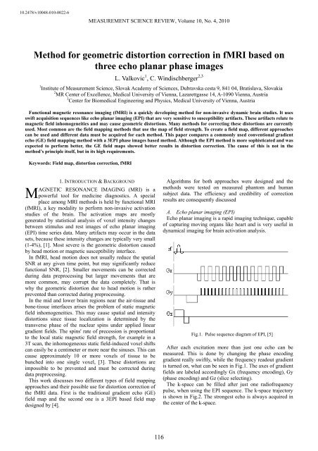
A. Echo planar imag<str<strong>on</strong>g>in</str<strong>on</strong>g>g (EPI)<br />
Echo planar imag<str<strong>on</strong>g>in</str<strong>on</strong>g>g is a rapid imag<str<strong>on</strong>g>in</str<strong>on</strong>g>g technique, capable<br />
of captur<str<strong>on</strong>g>in</str<strong>on</strong>g>g mov<str<strong>on</strong>g>in</str<strong>on</strong>g>g organs like heart and is very useful <str<strong>on</strong>g>in</str<strong>on</strong>g><br />
dynamical imag<str<strong>on</strong>g>in</str<strong>on</strong>g>g <str<strong>on</strong>g>for</str<strong>on</strong>g> bra<str<strong>on</strong>g>in</str<strong>on</strong>g> activati<strong>on</strong> analysis.<br />
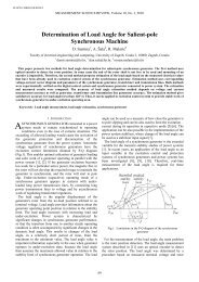
Fig.1. Pulse sequence diagram of EPI, [5]<br />
After each excitati<strong>on</strong> more than just <strong>on</strong>e echo can be<br />
measured. This is d<strong>on</strong>e by chang<str<strong>on</strong>g>in</str<strong>on</strong>g>g the phase encod<str<strong>on</strong>g>in</str<strong>on</strong>g>g<br />
gradient really swiftly, while the frequency readout gradient<br />
is turned <strong>on</strong>, what can be seen <str<strong>on</strong>g>in</str<strong>on</strong>g> Fig.1. The axes of gradient<br />
fields are labeled accord<str<strong>on</strong>g>in</str<strong>on</strong>g>gly Gx (frequency encod<str<strong>on</strong>g>in</str<strong>on</strong>g>g), Gy<br />
(phase encod<str<strong>on</strong>g>in</str<strong>on</strong>g>g) and Gz (slice select<str<strong>on</strong>g>in</str<strong>on</strong>g>g).<br />
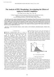
The k-space can be filled after just <strong>on</strong>e radiofrequency<br />
pulse, when us<str<strong>on</strong>g>in</str<strong>on</strong>g>g the EPI sequence. The k-space trajectory<br />
is shown <str<strong>on</strong>g>in</str<strong>on</strong>g> Fig.2. The str<strong>on</strong>gest echo is always acquired <str<strong>on</strong>g>in</str<strong>on</strong>g><br />
the center of the k-space.<br />
116
MEASUREMENT SCIENCE REVIEW, Volume 10, No. 4, 2010<br />
E. EPI field map<br />
Field maps calculated from EPI images are already<br />
distorted the same way as the rest of the data. This makes<br />
the <str<strong>on</strong>g>correcti<strong>on</strong></str<strong>on</strong>g> procedure easier and, more importantly, it<br />
takes much shorter time scann<str<strong>on</strong>g>in</str<strong>on</strong>g>g and the comput<str<strong>on</strong>g>in</str<strong>on</strong>g>g time is<br />
reas<strong>on</strong>able. But <strong>on</strong> the other hand these field maps must be<br />
computed manually dur<str<strong>on</strong>g>in</str<strong>on</strong>g>g the data preprocess<str<strong>on</strong>g>in</str<strong>on</strong>g>g <str<strong>on</strong>g>in</str<strong>on</strong>g>clud<str<strong>on</strong>g>in</str<strong>on</strong>g>g<br />
bra<str<strong>on</strong>g>in</str<strong>on</strong>g> mask<str<strong>on</strong>g>in</str<strong>on</strong>g>g, phase-unwrapp<str<strong>on</strong>g>in</str<strong>on</strong>g>g, calculati<strong>on</strong> of field<br />
strength and f<str<strong>on</strong>g>in</str<strong>on</strong>g>al smooth<str<strong>on</strong>g>in</str<strong>on</strong>g>g. All methods, which use EPI<br />
phase images to calculate field maps and are able to per<str<strong>on</strong>g>for</str<strong>on</strong>g>m<br />
phase-unwrapp<str<strong>on</strong>g>in</str<strong>on</strong>g>g assume l<str<strong>on</strong>g>in</str<strong>on</strong>g>ear or almost l<str<strong>on</strong>g>in</str<strong>on</strong>g>ear phase<br />
change over time, [4], [10].<br />
Fig.2. The k-space trajectory of EPI sequence<br />
B. EPI <str<strong>on</strong>g>geometric</str<strong>on</strong>g> <str<strong>on</strong>g>distorti<strong>on</strong></str<strong>on</strong>g><br />
Bra<str<strong>on</strong>g>in</str<strong>on</strong>g> EPI data are mostly rec<strong>on</strong>structed without <str<strong>on</strong>g>correcti<strong>on</strong></str<strong>on</strong>g><br />
of field <str<strong>on</strong>g>in</str<strong>on</strong>g>homogeneities, hence <str<strong>on</strong>g>geometric</str<strong>on</strong>g> <str<strong>on</strong>g>distorti<strong>on</strong></str<strong>on</strong>g>s are<br />
observed. These <str<strong>on</strong>g>distorti<strong>on</strong></str<strong>on</strong>g>s appear ma<str<strong>on</strong>g>in</str<strong>on</strong>g>ly at the boundaries<br />
of regi<strong>on</strong>s with significant magnetic susceptibility<br />
differences. In EPI, field <str<strong>on</strong>g>in</str<strong>on</strong>g>homogeneity causes pixel shifts<br />
and under severe c<strong>on</strong>diti<strong>on</strong>s may also lead to signal loss. A<br />
l<strong>on</strong>g readout time makes the system more sensitive <str<strong>on</strong>g>for</str<strong>on</strong>g><br />
<str<strong>on</strong>g>geometric</str<strong>on</strong>g> <str<strong>on</strong>g>distorti<strong>on</strong></str<strong>on</strong>g>s, ma<str<strong>on</strong>g>in</str<strong>on</strong>g>ly <str<strong>on</strong>g>in</str<strong>on</strong>g> phase encod<str<strong>on</strong>g>in</str<strong>on</strong>g>g directi<strong>on</strong>,<br />
[6]-[8]. These shifts depend <strong>on</strong> EPI slice readout time and<br />
the po<str<strong>on</strong>g>in</str<strong>on</strong>g>t field <str<strong>on</strong>g>in</str<strong>on</strong>g>homogeneity.<br />
C. Field maps<br />
S<str<strong>on</strong>g>in</str<strong>on</strong>g>ce <str<strong>on</strong>g>geometric</str<strong>on</strong>g> <str<strong>on</strong>g>distorti<strong>on</strong></str<strong>on</strong>g>s relate to field <str<strong>on</strong>g>in</str<strong>on</strong>g>homogeneities,<br />
us<str<strong>on</strong>g>in</str<strong>on</strong>g>g a map of magnetic field strength <str<strong>on</strong>g>in</str<strong>on</strong>g> a reverse process<br />
is a logical outcome, [9]. Field <str<strong>on</strong>g>in</str<strong>on</strong>g>homogeneity (ΔB) relates<br />
to the phase change <str<strong>on</strong>g>in</str<strong>on</strong>g> time accord<str<strong>on</strong>g>in</str<strong>on</strong>g>g to equati<strong>on</strong><br />
ΔΦ<br />
ΔB<br />
= − , (1)<br />
γΔTE<br />
where ΔΦ is the phase difference, γ is gyromagnetic ratio<br />
and ΔTE is difference <str<strong>on</strong>g>in</str<strong>on</strong>g> echo times.<br />
Two or more phase images must be acquired at different<br />
echo times (TE), but the differences between the <str<strong>on</strong>g>in</str<strong>on</strong>g>dividual<br />
TEs should be small enough to avoid phase-wrapp<str<strong>on</strong>g>in</str<strong>on</strong>g>g,<br />
otherwise a phase-unwrapp<str<strong>on</strong>g>in</str<strong>on</strong>g>g operati<strong>on</strong> is required.<br />
D. GE field map<br />
GE field map is a comm<strong>on</strong>ly used type of field map<br />
usually generated by the scanner automatically and<br />
immediately after data acquisiti<strong>on</strong>. It is usually computed<br />
from two GE phase images scanned at different echo times<br />
and the magnitude images are used to create a bra<str<strong>on</strong>g>in</str<strong>on</strong>g> mask.<br />
Phase-unwrapp<str<strong>on</strong>g>in</str<strong>on</strong>g>g is a standard procedure also d<strong>on</strong>e<br />
automatically by the scanner. As GE field map is<br />
anatomically and <str<strong>on</strong>g>geometric</str<strong>on</strong>g>ally correct, it must be distorted<br />
the same way as the EPI data first, be<str<strong>on</strong>g>for</str<strong>on</strong>g>e it can be used to<br />
correct the EPI data. The other drawback of this approach<br />
may be the l<strong>on</strong>ger acquisiti<strong>on</strong> time and possible artifacts<br />
from the necessary <str<strong>on</strong>g>distorti<strong>on</strong></str<strong>on</strong>g>. While full EPI image of the<br />
human bra<str<strong>on</strong>g>in</str<strong>on</strong>g> takes <strong>on</strong>ly a few sec<strong>on</strong>ds, the c<strong>on</strong>venti<strong>on</strong>al GE<br />
image requires several m<str<strong>on</strong>g>in</str<strong>on</strong>g>utes, [3].<br />
2. MATERIALS AND METHODS<br />
A. Image acquisiti<strong>on</strong><br />
EPI image series of phantom (3.75g NISO 4 x 6H 2 O + 5g<br />
NaCl <str<strong>on</strong>g>in</str<strong>on</strong>g> 1l of distilled water) and subject data were<br />
measured several times with different TE sub<str<strong>on</strong>g>in</str<strong>on</strong>g>tervals, from<br />
the ma<str<strong>on</strong>g>in</str<strong>on</strong>g> <str<strong>on</strong>g>in</str<strong>on</strong>g>terval 23ms to 42ms (ΔTE=1ms), so that many<br />
different field map estimati<strong>on</strong>s could be calculated. Both<br />
phase and magnitude <str<strong>on</strong>g>in</str<strong>on</strong>g>-vivo (resp. phantom) EPI images of<br />
k-space matrix size 96 x 96 (96 x 96), image matrix size 210<br />
x 210 (1050 x 1050) and 14 slices of thickness 4mm<br />
(2.5mm) were acquired with the measurement parameters<br />
set as follows, TR=400ms (2000ms), FOV=210*210<br />
(1050*1050) and the BW=260pixel/Hz (1580pixel/Hz).<br />
Phased array head coils with 8 and 16-channels were used to<br />
evaluate possible differences. For the first test measurement<br />
the phantom was artificially distorted <str<strong>on</strong>g>in</str<strong>on</strong>g> phase encod<str<strong>on</strong>g>in</str<strong>on</strong>g>g<br />
directi<strong>on</strong> by chang<str<strong>on</strong>g>in</str<strong>on</strong>g>g the shimm<str<strong>on</strong>g>in</str<strong>on</strong>g>g parameters, to simulate<br />
really big <str<strong>on</strong>g>geometric</str<strong>on</strong>g> <str<strong>on</strong>g>distorti<strong>on</strong></str<strong>on</strong>g>s. As the GE field map is<br />
comm<strong>on</strong>ly used <str<strong>on</strong>g>for</str<strong>on</strong>g> <str<strong>on</strong>g>distorti<strong>on</strong></str<strong>on</strong>g> <str<strong>on</strong>g>correcti<strong>on</strong></str<strong>on</strong>g>, <strong>on</strong>ly GE phase<br />
maps of subjects were acquired. The measurement<br />
parameters <str<strong>on</strong>g>for</str<strong>on</strong>g> the GE images were set as <str<strong>on</strong>g>for</str<strong>on</strong>g> the EPI data,<br />
<strong>on</strong>ly the ΔTE was 5.19ms.<br />
B. Field map calculated out of 3EPI images, [4]<br />
This method is unique by its approach to phaseunwrapp<str<strong>on</strong>g>in</str<strong>on</strong>g>g,<br />
where just 3EPI phase images with different<br />
TEs are used to calculate the phase-wraps correctly. The<br />
<str<strong>on</strong>g>in</str<strong>on</strong>g>terval between the first and the last TE must be chosen<br />
accord<str<strong>on</strong>g>in</str<strong>on</strong>g>gly to the field strength and also equati<strong>on</strong> (2) must<br />
apply so that just <strong>on</strong>e phase-wrap may occur <str<strong>on</strong>g>in</str<strong>on</strong>g> that <str<strong>on</strong>g>in</str<strong>on</strong>g>terval,<br />
<str<strong>on</strong>g>in</str<strong>on</strong>g> our experiments ΔTE 1,3 was 3ms.<br />
Δ TE<br />
(2)<br />
2,3<br />
= 2ΔTE1,2<br />
S<str<strong>on</strong>g>in</str<strong>on</strong>g>ce maximally <strong>on</strong>e phase-wrap may emerge, there are<br />
<strong>on</strong>ly 7 possible phase evoluti<strong>on</strong>s <str<strong>on</strong>g>for</str<strong>on</strong>g> each voxel. Each of<br />
these are calculated and l<str<strong>on</strong>g>in</str<strong>on</strong>g>early fitted and the evoluti<strong>on</strong><br />
with the best fit is chosen as the real <strong>on</strong>e. This way all<br />
phase-wraps are covered and the field map can be filtered<br />
and spatially smoothed <str<strong>on</strong>g>for</str<strong>on</strong>g> further use.<br />
All measurements were per<str<strong>on</strong>g>for</str<strong>on</strong>g>med <strong>on</strong> the 3T<br />
MAGNETOM Trio (Siemens AG, Erlangen, Germany).<br />
Programs <str<strong>on</strong>g>for</str<strong>on</strong>g> field map calculati<strong>on</strong> were developed <str<strong>on</strong>g>in</str<strong>on</strong>g><br />
MATLAB (MathWorks, Natick, Massachusetts). Field maps<br />
were c<strong>on</strong>verted <str<strong>on</strong>g>in</str<strong>on</strong>g>to voxel shift maps <str<strong>on</strong>g>for</str<strong>on</strong>g> <str<strong>on</strong>g>distorti<strong>on</strong></str<strong>on</strong>g><br />
117
MEASUREMENT SCIENCE REVIEW, Volume 10, No. 4, 2010<br />
<str<strong>on</strong>g>correcti<strong>on</strong></str<strong>on</strong>g>. Corrected images were compared with the<br />
structural bra<str<strong>on</strong>g>in</str<strong>on</strong>g> images of the same subjects, with the<br />
statistical parametric mapp<str<strong>on</strong>g>in</str<strong>on</strong>g>g (SPM) program, [11].<br />
3. RESULTS AND DISCUSSION<br />
As described above, EPI magnitude and phase images<br />
were acquired, al<strong>on</strong>g with GE magnitude images and phase<br />
maps. C<strong>on</strong>sequently, field maps were calculated from the<br />
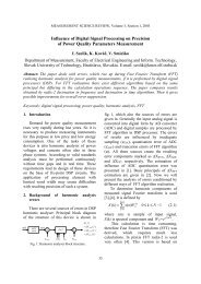
acquired data sets. Dem<strong>on</strong>strati<strong>on</strong> of the 3EPI <str<strong>on</strong>g>based</str<strong>on</strong>g> field<br />
mapp<str<strong>on</strong>g>in</str<strong>on</strong>g>g method is shown <str<strong>on</strong>g>in</str<strong>on</strong>g> Fig.3. The shape of the<br />
corrected phantom image is very similar to the not distorted<br />
image, and even though the <str<strong>on</strong>g>correcti<strong>on</strong></str<strong>on</strong>g> is not perfect, <str<strong>on</strong>g>for</str<strong>on</strong>g><br />
artificial <str<strong>on</strong>g>distorti<strong>on</strong></str<strong>on</strong>g>s the method shows good results <strong>on</strong> the<br />
phantom data.<br />
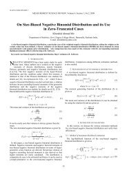
The comparis<strong>on</strong> of the two studied methods is shown <strong>on</strong><br />
subject data <str<strong>on</strong>g>in</str<strong>on</strong>g> Fig.4: In the a) image is a structural axial<br />
slice of a human bra<str<strong>on</strong>g>in</str<strong>on</strong>g>; the same bra<str<strong>on</strong>g>in</str<strong>on</strong>g> slice, but measured<br />
us<str<strong>on</strong>g>in</str<strong>on</strong>g>g EPI scann<str<strong>on</strong>g>in</str<strong>on</strong>g>g sequence with a visible <str<strong>on</strong>g>geometric</str<strong>on</strong>g><br />
<str<strong>on</strong>g>distorti<strong>on</strong></str<strong>on</strong>g>s is shown <str<strong>on</strong>g>in</str<strong>on</strong>g> the b) image; after apply<str<strong>on</strong>g>in</str<strong>on</strong>g>g the 3EPI<br />
field map <str<strong>on</strong>g>for</str<strong>on</strong>g> <str<strong>on</strong>g>distorti<strong>on</strong></str<strong>on</strong>g> <str<strong>on</strong>g>correcti<strong>on</strong></str<strong>on</strong>g> almost no pixel shifts<br />
were per<str<strong>on</strong>g>for</str<strong>on</strong>g>med as is shown <str<strong>on</strong>g>in</str<strong>on</strong>g> the c) image; the GE field<br />
map was also used and with better results, image d) shows<br />
the EPI scan after <str<strong>on</strong>g>distorti<strong>on</strong></str<strong>on</strong>g> <str<strong>on</strong>g>correcti<strong>on</strong></str<strong>on</strong>g> d<strong>on</strong>e us<str<strong>on</strong>g>in</str<strong>on</strong>g>g the GE<br />
field map.<br />
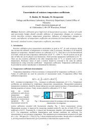
Fig.3. Dem<strong>on</strong>strati<strong>on</strong> of 3EPI <str<strong>on</strong>g>based</str<strong>on</strong>g> field mapp<str<strong>on</strong>g>in</str<strong>on</strong>g>g method <strong>on</strong> phantom images. On the left is a phantom image without <str<strong>on</strong>g>distorti<strong>on</strong></str<strong>on</strong>g>,<br />
image <str<strong>on</strong>g>in</str<strong>on</strong>g> the middle shows distorted phantom and <strong>on</strong> the right is the phantom image after <str<strong>on</strong>g>distorti<strong>on</strong></str<strong>on</strong>g> <str<strong>on</strong>g>correcti<strong>on</strong></str<strong>on</strong>g> us<str<strong>on</strong>g>in</str<strong>on</strong>g>g the 3EPI<br />
<str<strong>on</strong>g>based</str<strong>on</strong>g> field mapp<str<strong>on</strong>g>in</str<strong>on</strong>g>g method.<br />
Fig.4. Comparis<strong>on</strong> of EPI and GE field mapp<str<strong>on</strong>g>in</str<strong>on</strong>g>g <str<strong>on</strong>g>distorti<strong>on</strong></str<strong>on</strong>g> <str<strong>on</strong>g>correcti<strong>on</strong></str<strong>on</strong>g>. This figure shows 4 axial slices of the subject bra<str<strong>on</strong>g>in</str<strong>on</strong>g>. Image<br />
a) shows the structural image of the bra<str<strong>on</strong>g>in</str<strong>on</strong>g>, image b) is the EPI scan of this bra<str<strong>on</strong>g>in</str<strong>on</strong>g>. The <str<strong>on</strong>g>distorti<strong>on</strong></str<strong>on</strong>g> of the image is visible <str<strong>on</strong>g>in</str<strong>on</strong>g> the fr<strong>on</strong>t<br />
of the bra<str<strong>on</strong>g>in</str<strong>on</strong>g>. Field map <str<strong>on</strong>g>distorti<strong>on</strong></str<strong>on</strong>g> <str<strong>on</strong>g>correcti<strong>on</strong></str<strong>on</strong>g> methods were used. In image c) is the bra<str<strong>on</strong>g>in</str<strong>on</strong>g> after EPI field map <str<strong>on</strong>g>correcti<strong>on</strong></str<strong>on</strong>g> and <str<strong>on</strong>g>in</str<strong>on</strong>g><br />
image d) is the bra<str<strong>on</strong>g>in</str<strong>on</strong>g> after GE field map <str<strong>on</strong>g>correcti<strong>on</strong></str<strong>on</strong>g>.<br />
118
MEASUREMENT SCIENCE REVIEW, Volume 10, No. 4, 2010<br />
2<br />
1.9<br />
Phase value [rad]<br />
1.8<br />
1.7<br />
1.6<br />
1.5<br />
1.4<br />
0.024 0.026 0.028 0.03 0.032 0.034<br />
TE [s]<br />
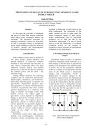
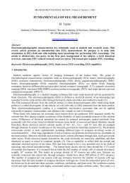
Fig.5. Phase evoluti<strong>on</strong> <str<strong>on</strong>g>in</str<strong>on</strong>g> time of <strong>three</strong> different randomly chosen voxels of the measured phantom EPI phase images. The phase<br />
does not evolve <str<strong>on</strong>g>in</str<strong>on</strong>g> time l<str<strong>on</strong>g>in</str<strong>on</strong>g>early not even almost l<str<strong>on</strong>g>in</str<strong>on</strong>g>early, the phase fluctuati<strong>on</strong>s that occur are not even the same <str<strong>on</strong>g>for</str<strong>on</strong>g> every voxel<br />
of the phantom.<br />
There is a mean<str<strong>on</strong>g>in</str<strong>on</strong>g>gful explanati<strong>on</strong> why the GE <str<strong>on</strong>g>based</str<strong>on</strong>g> field<br />
mapp<str<strong>on</strong>g>in</str<strong>on</strong>g>g method shows better results than the 3EPI <str<strong>on</strong>g>based</str<strong>on</strong>g><br />
method, as can be seen <str<strong>on</strong>g>in</str<strong>on</strong>g> Fig.4. The acquired data sets do<br />
not fulfill the ma<str<strong>on</strong>g>in</str<strong>on</strong>g> and essential requirement <str<strong>on</strong>g>for</str<strong>on</strong>g> the EPI<br />
method to work correctly. Namely the l<str<strong>on</strong>g>in</str<strong>on</strong>g>ear or almost l<str<strong>on</strong>g>in</str<strong>on</strong>g>ear<br />
phase evoluti<strong>on</strong> <str<strong>on</strong>g>in</str<strong>on</strong>g> time. Fig.5 shows the time evoluti<strong>on</strong> of<br />
phase <str<strong>on</strong>g>for</str<strong>on</strong>g> <strong>three</strong> different, randomly chosen voxels of the<br />
phantom data. The phase evoluti<strong>on</strong> measured is not l<str<strong>on</strong>g>in</str<strong>on</strong>g>ear,<br />
many phase fluctuati<strong>on</strong>s occur <str<strong>on</strong>g>in</str<strong>on</strong>g> the studied <str<strong>on</strong>g>in</str<strong>on</strong>g>terval. With<br />
this k<str<strong>on</strong>g>in</str<strong>on</strong>g>d of phase evoluti<strong>on</strong>, the l<str<strong>on</strong>g>in</str<strong>on</strong>g>ear fitt<str<strong>on</strong>g>in</str<strong>on</strong>g>g algorithm <str<strong>on</strong>g>for</str<strong>on</strong>g><br />
phase-unwrapp<str<strong>on</strong>g>in</str<strong>on</strong>g>g is absolutely <str<strong>on</strong>g>in</str<strong>on</strong>g>adequate.<br />
Field maps calculated us<str<strong>on</strong>g>in</str<strong>on</strong>g>g data sets with n<strong>on</strong>-l<str<strong>on</strong>g>in</str<strong>on</strong>g>ear<br />
phase evoluti<strong>on</strong> <str<strong>on</strong>g>in</str<strong>on</strong>g> time cannot be calculated correctly. This<br />
significant miscalculati<strong>on</strong> makes these magnetic field maps<br />
<str<strong>on</strong>g>in</str<strong>on</strong>g>efficient <str<strong>on</strong>g>for</str<strong>on</strong>g> <str<strong>on</strong>g>geometric</str<strong>on</strong>g> <str<strong>on</strong>g>distorti<strong>on</strong></str<strong>on</strong>g> <str<strong>on</strong>g>correcti<strong>on</strong></str<strong>on</strong>g>. There<str<strong>on</strong>g>for</str<strong>on</strong>g>e,<br />
be<str<strong>on</strong>g>for</str<strong>on</strong>g>e us<str<strong>on</strong>g>in</str<strong>on</strong>g>g any EPI <str<strong>on</strong>g>based</str<strong>on</strong>g> field mapp<str<strong>on</strong>g>in</str<strong>on</strong>g>g method, no matter<br />
how sophisticated its ma<str<strong>on</strong>g>in</str<strong>on</strong>g> pr<str<strong>on</strong>g>in</str<strong>on</strong>g>ciple is, it is highly<br />
recommended to check first if the key requirements are<br />
fulfilled.<br />
4. CONCLUSIONS<br />
Two different magnetic field mapp<str<strong>on</strong>g>in</str<strong>on</strong>g>g methods were used<br />
<str<strong>on</strong>g>for</str<strong>on</strong>g> <str<strong>on</strong>g>geometric</str<strong>on</strong>g> <str<strong>on</strong>g>distorti<strong>on</strong></str<strong>on</strong>g> <str<strong>on</strong>g>correcti<strong>on</strong></str<strong>on</strong>g>. Both methods have been<br />
evaluated <strong>on</strong> acquired phantom and subject data sets. EPI<br />
field mapp<str<strong>on</strong>g>in</str<strong>on</strong>g>g method is <str<strong>on</strong>g>in</str<strong>on</strong>g> general more sophisticated and<br />
has many advantages, but s<str<strong>on</strong>g>in</str<strong>on</strong>g>ce the phase did not evolve<br />
l<str<strong>on</strong>g>in</str<strong>on</strong>g>early or almost l<str<strong>on</strong>g>in</str<strong>on</strong>g>early, it did not show reliable results.<br />
S<str<strong>on</strong>g>in</str<strong>on</strong>g>ce the ma<str<strong>on</strong>g>in</str<strong>on</strong>g> requirement <str<strong>on</strong>g>for</str<strong>on</strong>g> right calculati<strong>on</strong> of EPI<br />
<str<strong>on</strong>g>based</str<strong>on</strong>g> field map was not fulfilled, the GE field map used <str<strong>on</strong>g>for</str<strong>on</strong>g><br />
the same purpose showed better results and is there<str<strong>on</strong>g>for</str<strong>on</strong>g>e<br />
c<strong>on</strong>sidered to be more robust.<br />
ACKNOWLEDGMENTS<br />
This work was supported <str<strong>on</strong>g>in</str<strong>on</strong>g> part by the Tatra Bank<br />
Foundati<strong>on</strong> grant <str<strong>on</strong>g>for</str<strong>on</strong>g> students work abroad 2008sds091 and<br />
<str<strong>on</strong>g>in</str<strong>on</strong>g> part by Slovak Scientific Grant Agency VEGA 2/0142/08.<br />
REFERENCES<br />
[1] Yeo, D.T.B., Fessler, J.A., Kim, B. (2008). C<strong>on</strong>current<br />
<str<strong>on</strong>g>correcti<strong>on</strong></str<strong>on</strong>g> of <str<strong>on</strong>g>geometric</str<strong>on</strong>g> <str<strong>on</strong>g>distorti<strong>on</strong></str<strong>on</strong>g> and moti<strong>on</strong> us<str<strong>on</strong>g>in</str<strong>on</strong>g>g the<br />
map-slice-to-volume method <str<strong>on</strong>g>in</str<strong>on</strong>g> echo-planar imag<str<strong>on</strong>g>in</str<strong>on</strong>g>g.<br />
Magn. Res<strong>on</strong>. Imag<str<strong>on</strong>g>in</str<strong>on</strong>g>g, 26, 703-714.<br />
[2] Huettel, S.A., S<strong>on</strong>g, A.W., McCarthy, G. (2009).<br />
Functi<strong>on</strong>al Magnetic Res<strong>on</strong>ance Imag<str<strong>on</strong>g>in</str<strong>on</strong>g>g. Sunderland:<br />
S<str<strong>on</strong>g>in</str<strong>on</strong>g>auer Associates.<br />
[3] Holland, D., Kuperman, J.M., Dale, A.M. (2010).<br />
Efficient <str<strong>on</strong>g>correcti<strong>on</strong></str<strong>on</strong>g> of <str<strong>on</strong>g>in</str<strong>on</strong>g>homogeneous static magnetic<br />
field-<str<strong>on</strong>g>in</str<strong>on</strong>g>duced <str<strong>on</strong>g>distorti<strong>on</strong></str<strong>on</strong>g> <str<strong>on</strong>g>in</str<strong>on</strong>g> Echo Planar Imag<str<strong>on</strong>g>in</str<strong>on</strong>g>g.<br />
NeuroImage, 50 (1), 175-183.<br />
[4] W<str<strong>on</strong>g>in</str<strong>on</strong>g>dischberger, C., Rob<str<strong>on</strong>g>in</str<strong>on</strong>g>s<strong>on</strong>, S., Rauscher, A., Barth,<br />
M., Moser, E. (2004). Robust field map generati<strong>on</strong><br />
us<str<strong>on</strong>g>in</str<strong>on</strong>g>g a triple-echo acquisiti<strong>on</strong>. J. Magn. Res<strong>on</strong>.<br />
Imag<str<strong>on</strong>g>in</str<strong>on</strong>g>g, 20, 730-734.<br />
[5] Stuart, C. (1997). Functi<strong>on</strong>al MRI: <str<strong>on</strong>g>Method</str<strong>on</strong>g>s and<br />
Applicati<strong>on</strong>s. Doctoral thesis, University of<br />
Nott<str<strong>on</strong>g>in</str<strong>on</strong>g>gham.<br />
[6] Jezzard, P., Balaban, R.S. (1995). Correcti<strong>on</strong> <str<strong>on</strong>g>for</str<strong>on</strong>g><br />
<str<strong>on</strong>g>geometric</str<strong>on</strong>g> <str<strong>on</strong>g>distorti<strong>on</strong></str<strong>on</strong>g> <str<strong>on</strong>g>in</str<strong>on</strong>g> echo planar images from B0<br />
field variati<strong>on</strong>s. Magn. Res<strong>on</strong>. Med., 34, 65-73.<br />
[7] Kadah, Y.M., Hu, X. (1998). Algebraic rec<strong>on</strong>structi<strong>on</strong><br />
<str<strong>on</strong>g>for</str<strong>on</strong>g> magnetic res<strong>on</strong>ance imag<str<strong>on</strong>g>in</str<strong>on</strong>g>g under B0<br />
<str<strong>on</strong>g>in</str<strong>on</strong>g>homogeneity. IEEE Trans. Med. Imag<str<strong>on</strong>g>in</str<strong>on</strong>g>g, 17,<br />
362-370.<br />
[8] Jezzard, P., Clare, S. (1999). Sources of <str<strong>on</strong>g>distorti<strong>on</strong></str<strong>on</strong>g> <str<strong>on</strong>g>in</str<strong>on</strong>g><br />
functi<strong>on</strong>al MRI data. Hum. Bra<str<strong>on</strong>g>in</str<strong>on</strong>g> Mapp., 8, 80-85.<br />
[9] Moghaddam, A.N., Soltanian-Zadeh, H. (2003).<br />
Mapp<str<strong>on</strong>g>in</str<strong>on</strong>g>g of magnetic field <str<strong>on</strong>g>in</str<strong>on</strong>g>homogeneity and removal<br />
of its artifact from MR images. In Medical Imag<str<strong>on</strong>g>in</str<strong>on</strong>g>g<br />
2003. Proceed<str<strong>on</strong>g>in</str<strong>on</strong>g>gs of SPIE, Vol. 5032, 780-787.<br />
[10] Reber, P.J., W<strong>on</strong>g, E.C., Buxt<strong>on</strong>, K.B., Frank, L.R.<br />
(1998). Correcti<strong>on</strong> of off-res<strong>on</strong>ance related <str<strong>on</strong>g>distorti<strong>on</strong></str<strong>on</strong>g><br />
<str<strong>on</strong>g>in</str<strong>on</strong>g> echo-planar imag<str<strong>on</strong>g>in</str<strong>on</strong>g>g us<str<strong>on</strong>g>in</str<strong>on</strong>g>g EPI-<str<strong>on</strong>g>based</str<strong>on</strong>g> field maps.<br />
Magn. Res<strong>on</strong>. Med., 39, 328-330.<br />
[11] SPM – Statistical Parametric Mapp<str<strong>on</strong>g>in</str<strong>on</strong>g>g,<br />
http://www.fil.i<strong>on</strong>.ucl.ac.uk/spm<br />
Received March 25, 2010. Accepted October 18, 2010.<br />
119