Data Structures and Algorithms in Java[1].pdf - Fulvio Frisone

Data Structures and Algorithms in Java
Michael T. Goodrich
Department of Computer Science University of California, Irvine
1

Roberto Tamassia
Department of Computer Science Brown University
0-471-73884-0
Fourth Edition
John Wiley & Sons, Inc.
ASSOCIATE PUBLISHER
MARKETING DIRECTOR
EDITORIAL ASSISTANT
SENIOR PRODUCTION EDITOR
COVER DESIGNER
COVER PHOTO RESEARCHER
Dan Sayre
Frank Lyman
Bridget Morrisey
Ken Santor
Hope Miller
Lisa Gee
Clevenger/Corbis
COVER PHOTO Ralph A.
This book was set in by the authors and printed and bound by R.R. Donnelley
- Crawfordsville. The cover was printed by Phoenix Color, Inc.
Front Matter
To Karen, Paul, Anna, and Jack
-Michael T. Goodrich
2

To Isabel
-Roberto Tamassia
Preface to the Fourth Edition
This fourth edition is designed to provide an introduction to data structures and
algorithms, including their design, analysis, and implementation. In terms of curricula
based on the IEEE/ACM 2001 Computing Curriculum, this book is appropriate for
use in the courses CS102 (I/O/B versions), CS103 (I/O/B versions), CS111 (A
version), and CS112 (A/I/O/F/H versions). We discuss its use for such courses in
more detail later in this preface.
The major changes, with respect to the third edition, are the following:
• Added new chapter on arrays, linked lists, and recursion.
• Added new chapter on memory management.
• Full integration with Java 5.0.
• Better integration with the Java Collections Framework.
• Better coverage of iterators.
• Increased coverage of array lists, including the replacement of uses of the class
java.util.Vector with java.util.ArrayList.
• Update of all Java APIs to use generic types.
• Simplified list, binary tree, and priority queue ADTs.
• Further streamlining of mathematics to the seven most used functions.
• Expanded and revised exercises, bringing the total number of reinforcement,
creativity, and project exercises to 670. Added exercises include new projects on
maintaining a game's high-score list, evaluating postfix and infix expressions,
minimax game-tree evaluation, processing stock buy and sell orders, scheduling
CPU jobs, n-body simulation, computing DNA-strand edit distance, and creating
and solving mazes.
This book is related to the following books:
• M.T. Goodrich, R. Tamassia, and D.M. Mount, Data Structures and Algorithms
in C++, John Wiley & Sons, Inc., 2004. This book has a similar overall structure to
the present book, but uses C++ as the underlying language (with some modest, but
necessary pedagogical differences required by this approach). Thus, it could make
3

for a handy companion book in a curriculum that allows for either a Java or C++
track in the introductory courses.
• M.T. Goodrich and R. Tamassia, Algorithm Design: Foundations, Analysis, and
Internet Examples, John Wiley & Sons, Inc., 2002. This is a textbook for a more
advanced algorithms and data structures course, such as CS210 (T/W/C/S versions)
in the IEEE/ACM 2001 curriculum.
Use as a Textbook
The design and analysis of efficient data structures has long been recognized as a
vital subject in computing, for the study of data structures is part of the core of
every collegiate computer science and computer engineering major program we are
familiar with. Typically, the introductory courses are presented as a two- or threecourse
sequence. Elementary data structures are often briefly introduced in the first
programming or introduction to computer science course and this is followed by a
more in-depth introduction to data structures in the following course(s).
Furthermore, this course sequence is typically followed at a later point in the
curriculum by a more in-depth study of data structures and algorithms. We feel that
the central role of data structure design and analysis in the curriculum is fully
justified, given the importance of efficient data structures in most software systems,
including the Web, operating systems, databases, compilers, and scientific
simulation systems.
With the emergence of the object-oriented paradigm as the framework of choice for
building robust and reusable software, we have tried to take a consistent
objectoriented viewpoint throughout this text. One of the main ideas of the objectoriented
approach is that data should be presented as being encapsulated with the
methods that access and modify them. That is, rather than simply viewing data as a
collection of bytes and addresses, we think of data as instances of an abstract data
type (ADT) that include a repertory of methods for performing operations on the
data. Likewise, object-oriented solutions are often organized utilizing common
design patterns, which facilitate software reuse and robustness. Thus, we present
each data structure using ADTs and their respective implementations and we
introduce important design patterns as means to organize those implementations
into classes, methods, and objects.
For each ADT presented in this book, we provide an associated Java interface.
Also, concrete data structures realizing the ADTs are provided as Java classes
implementing the interfaces above. We also give Java implementations of
fundamental algorithms (such as sorting and graph traversals) and of sample
applications of data structures (such as HTML tag matching and a photo album).
Due to space limitations, we sometimes show only code fragments in the book and
make additional source code available on the companion Web site,
http://java.datastructures.net.
4

The Java code implementing fundamental data structures in this book is organized
in a single Java package, net.datastructures. This package forms a coherent library
of data structures and algorithms in Java specifically designed for educational
purposes in a way that is complementary with the Java Collections Framework.
Web Added-Value Education
This book is accompanied by an extensive Web site:
http://java.datastructures.net.
Students are encouraged to use this site along with the book, to help with exercises
and increase understanding of the subject. Instructors are likewise welcome to use
the site to help plan, organize, and present their course materials.
For the Student
for all readers, and specifically for students, we include:
• All the Java source code presented in this book.
• The student version of the net.datastructures package.
• Slide handouts (four-per-page) in PDF format.
• A database of hints to all exercises, indexed by problem number.
• Java animations and interactive applets for data structures and algorithms.
• Hyperlinks to other data structures and algorithms resources.
We feel that the Java animations and interactive applets should be of particular
interest, since they allow readers to interactively "play" with different data
structures, which leads to better understanding of the different ADTs. In addition,
the hints should be of considerable use to anyone needing a little help getting
started on certain exercises.
For the Instructor
For instructors using this book, we include the following additional teaching aids:
• Solutions to over two hundred of the book's exercises.
• A keyword-searchable database of additional exercises.
• The complete net.datastructures package.
5

• Additional Java source code.
• Slides in Powerpoint and PDF (one-per-page) format.
• Self-contained special-topic supplements, including discussions on convex
hulls, range trees, and orthogonal segment intersection.
The slides are fully editable, so as to allow an instructor using this book full
freedom in customizing his or her presentations.
A Resource for Teaching Data Structures and Algorithms
This book contains many Java-code and pseudo-code fragments, and over 670
exercises, which are divided into roughly 40% reinforcement exercises, 40%
creativity exercises, and 20% programming projects.
This book can be used for courses CS102 (I/O/B versions), CS103 (I/O/B versions),
CS111 (A version), and/or CS112 (A/I/O/F/H versions) in the IEEE/ACM 2001
Computing Curriculum, with instructional units as outlined in Table 0.1.
Table 0.1: Material for Units in the IEEE/ACM 2001
Computing Curriculum.
Instructional Unit
Relevant Material
PL1. Overview of Programming Languages
Chapters 1 & 2
PL2. Virtual Machines
Sections 14.1.1, 14.1.2, & 14.1.3
PL3. Introduction to Language Translation
Section 1.9
PL4. Declarations and Types
Sections 1.1, 2.4, & 2.5
PL5. Abstraction Mechanisms
Sections 2.4, 5.1, 5.2, 5.3, 6.1.1, 6.2, 6.4, 6.3, 7.1, 7.3.1, 8.1, 9.1, 9.3, 11.6,
& 13.1
6

PL6. Object-Oriented Programming
Chapters 1 & 2 and Sections 6.2.2, 6.3, 7.3.7, 8.1.2, & 13.3.1
PF1. Fundamental Programming Constructs
Chapters 1 & 2
PF2. Algorithms and Problem-Solving
Sections 1.9 & 4.2
PF3. Fundamental Data Structures
Sections 3.1, 5.1-3.2, 5.3, , 6.1-6.4, 7.1, 7.3, 8.1, 8.3, 9.1-9.4, 10.1, & 13.1
PF4. Recursion
Section 3.5
SE1. Software Design
Chapter 2 and Sections 6.2.2, 6.3, 7.3.7, 8.1.2, & 13.3.1
SE2. Using APIs
Sections 2.4, 5.1, 5.2, 5.3, 6.1.1, 6.2, 6.4, 6.3, 7.1, 7.3.1, 8.1, 9.1, 9.3, 11.6,
& 13.1
AL1. Basic Algorithmic Analysis
Chapter 4
AL2. Algorithmic Strategies
Sections 11.1.1, 11.7.1, 12.2.1, 12.4.2, & 12.5.2
AL3. Fundamental Computing Algorithms
Sections 8.1.4, 8.2.3, 8.3.5, 9.2, & 9.3.3, and Chapters 11, 12, & 13
DS1. Functions, Relations, and Sets
Sections 4.1, 8.1, & 11.6
DS3. Proof Techniques
Sections 4.3, 6.1.4, 7.3.3, 8.3, 10.2, 10.3, 10.4, 10.5, 11.2.1, 11.3, 11.6.2,
13.1, 13.3.1, 13.4, & 13.5
7

DS4. Basics of Counting
Sections 2.2.3 & 11.1.5
DS5. Graphs and Trees
Chapters 7, 8, 10, & 13
DS6. Discrete Probability
Appendix A and Sections 9.2.2, 9.4.2, 11.2.1, & 11.7
Chapter Listing
The chapters for this course are organized to provide a pedagogical path that starts
with the basics of Java programming and object-oriented design, moves to concrete
structures like arrays and linked lists, adds foundational techniques like recursion and
algorithm analysis, and then presents the fundamental data structures and algorithms,
concluding with a discussion of memory management (that is, the architectural
underpinnings of data structures). Specifically, the chapters for this book are
organized as follows:
1. Java Programming Basics
2. Object-Oriented Design
3. Arrays, Linked Lists, and Recursion
4. Analysis Tools
5. Stacks and Queues
6. Lists and Iterators
7. Trees
8. Priority Queues
9. Maps and Dictionaries
10. Search Trees
11. Sorting, Sets, and Selection
12. Text Processing
13. Graphs
8

14. Memory
A. Useful Mathematical Facts
Prerequisites
We have written this book assuming that the reader comes to it with certain
knowledge.That is, we assume that the reader is at least vaguely familiar with a
high-level programming language, such as C, C++, or Java, and that he or she
understands the main constructs from such a high-level language, including:
• Variables and expressions.
• Methods (also known as functions or procedures).
• Decision structures (such as if-statements and switch-statements).
• Iteration structures (for-loops and while-loops).
For readers who are familiar with these concepts, but not with how they are
expressed in Java, we provide a primer on the Java language in Chapter 1. Still, this
book is primarily a data structures book, not a Java book; hence, it does not provide
a comprehensive treatment of Java. Nevertheless, we do not assume that the reader
is necessarily familiar with object-oriented design or with linked structures, such as
linked lists, for these topics are covered in the core chapters of this book.
In terms of mathematical background, we assume the reader is somewhat familiar
with topics from high-school mathematics. Even so, in Chapter 4, we discuss the
seven most-important functions for algorithm analysis. In fact, sections that use
something other than one of these seven functions are considered optional, and are
indicated with a star (). We give a summary of other useful mathematical facts,
including elementary probability, in Appendix A.
About the Authors
Professors Goodrich and Tamassia are well-recognized researchers in algorithms
and data structures, having published many papers in this field, with applications to
Internet computing, information visualization, computer security, and geometric
computing. They have served as principal investigators in several joint projects
sponsored by the National Science Foundation, the Army Research Office, and the
9

Defense Advanced Research Projects Agency. They are also active in educational
technology research, with special emphasis on algorithm visualization systems.
Michael Goodrich received his Ph.D. in Computer Science from Purdue University
in 1987. He is currently a professor in the Department of Computer Science at
University of California, Irvine. Previously, he was a professor at Johns Hopkins
University. He is an editor for the International Journal of Computational
Geometry & Applications and Journal of Graph Algorithms and Applications.
Roberto Tamassia received his Ph.D. in Electrical and Computer Engineering from
the University of Illinois at Urbana-Champaign in 1988. He is currently a professor
in the Department of Computer Science at Brown University. He is editor-in-chief
for the Journal of Graph Algorithms and Applications and an editor for
Computational Geometry: Theory and Applications. He previously served on the
editorial board of IEEE Transactions on Computers.
In addition to their research accomplishments, the authors also have extensive
experience in the classroom. For example, Dr. Goodrich has taught data structures
and algorithms courses, including Data Structures as a freshman-sophomore level
course and Introduction to Algorithms as an upper level course. He has earned
several teaching awards in this capacity. His teaching style is to involve the students
in lively interactive classroom sessions that bring out the intuition and insights
behind data structuring and algorithmic techniques. Dr. Tamassia has taught Data
Structures and Algorithms as an introductory freshman-level course since 1988.
One thing that has set his teaching style apart is his effective use of interactive
hypermedia presentations integrated with the Web.
The instructional Web sites, datastructures.net and
algorithmdesign.net, supported by Drs. Goodrich and Tamassia, are used as
reference material by students, teachers, and professionals worldwide.
Acknowledgments
There are a number of individuals who have made contributions to this book.
We are grateful to all our research collaborators and teaching assistants, who
provided feedback on early drafts of chapters and have helped us in developing
exercises, programming assignments, and algorithm animation systems.In
particular, we would like to thank Jeff Achter, Vesselin Arnaudov, James Baker,
Ryan Baker,Benjamin Boer, Mike Boilen, Devin Borland, Lubomir Bourdev, Stina
Bridgeman, Bryan Cantrill, Yi-Jen Chiang, Robert Cohen, David Ellis, David
Emory, Jody Fanto, Ben Finkel, Ashim Garg, Natasha Gelfand, Mark Handy,
Michael Horn, Beno^it Hudson, Jovanna Ignatowicz, Seth Padowitz, James
Piechota, Dan Polivy, Seth Proctor, Susannah Raub, Haru Sakai, Andy Schwerin,
Michael Shapiro, MikeShim, Michael Shin, Galina Shubina, Christian Straub, Ye
10

Sun, Nikos Triandopoulos, Luca Vismara, Danfeng Yao, Jason Ye, and Eric
Zamore.
Lubomir Bourdev, Mike Demmer, Mark Handy, Michael Horn, and Scott Speigler
developed a basic Java tutorial, which ultimately led to Chapter 1, Java
Programming.
Special thanks go to Eric Zamore, who contributed to the development of the Java
code examples in this book and to the initial design, implementation, and testing of
the net.datastructures library of data structures and algorithms in Java. We are also
grateful to Vesselin Arnaudov and ike Shim for testing the current version of
net.datastructures
Many students and instructors have used the two previous editions of this book and
their experiences and responses have helped shape this fourth edition.
There have been a number of friends and colleagues whose comments have lead to
improvements in the text. We are particularly thankful to Karen Goodrich, Art
Moorshead, David Mount, Scott Smith, and Ioannis Tollis for their insightful
comments. In addition, contributions by David Mount to Section 3.5 and to several
figures are gratefully acknowledged.
We are also truly indebted to the outside reviewers and readers for their copious
comments, emails, and constructive criticism, which were extremely useful in
writing the fourth edition. We specifically thank the following reviewers for their
comments and suggestions: Divy Agarwal, University of California, Santa Barbara;
Terry Andres, University of Manitoba; Bobby Blumofe, University of Texas,
Austin; Michael Clancy, University of California, Berkeley; Larry Davis,
University of Maryland; Scott Drysdale, Dartmouth College; Arup Guha,
University of Central Florida; Chris Ingram, University of Waterloo; Stan Kwasny,
Washington University; Calvin Lin, University of Texas at Austin; John Mark
Mercer, McGill University; Laurent Michel, University of Connecticut; Leonard
Myers, California Polytechnic State University, San Luis Obispo; David Naumann,
Stevens Institute of Technology; Robert Pastel, Michigan Technological University;
Bina Ramamurthy, SUNY Buffalo; Ken Slonneger, University of Iowa; C.V.
Ravishankar, University of Michigan; Val Tannen, University of Pennsylvania;
Paul Van Arragon, Messiah College; and Christopher Wilson, University of
Oregon.
The team at Wiley has been great. Many thanks go to Lilian Brady, Paul Crockett,
Simon Durkin, Lisa Gee, Frank Lyman, Madelyn Lesure, Hope Miller, Bridget
Morrisey, Ken Santor, Dan Sayre, Bruce Spatz, Dawn Stanley, Jeri Warner, and
Bill Zobrist.
The computing systems and excellent technical support staff in the departments of
computer science at Brown University and University of California, Irvine gave us
reliable working environments. This manuscript was prepared primarily with the
11

typesetting package for the text and Adobe FrameMaker® and Microsoft
Visio® for the figures.
Finally, we would like to warmly thank Isabel Cruz, Karen Goodrich, Giuseppe Di
Battista, Franco Preparata, Ioannis Tollis, and our parents for providing advice,
encouragement, and support at various stages of the preparation of this book. We
also thank them for reminding us that there are things in life beyond writing books.
Michael T. Goodrich
Roberto Tamassia
Chapter 1
Java Programming Basics
Contents
1.1
12

Getting Started: Classes, Types, and Objects...
2
1.1.1
Base
Types.........................................................
..
5
1.1.2
Objects.......................................................
.......
7
1.1.3
Enum
Types.........................................................
.
14
1.2
Methods.......................................
15
1.3
Expressions...................................
20
1.3.1
Literals......................................................
......
20
1.3.2
Operators.....................................................
......
21
1.3.3
13

Casting and Autoboxing/Unboxing in
Expressions......................
25
1.4
Control Flow...................................
27
1.4.1
The If and Switch
Statements........................................
27
1.4.2
Loops.........................................................
......
29
1.4.3
Explicit Control-Flow
Statements....................................
32
1.5
Arrays.........................................
34
1.5.1
Declaring
Arrays....................................................
36
1.5.2
Arrays are
Objects..................................................
37
1.6
Simple Input and Output........................
14

39
1.7
An Example Program.............................
42
1.8
Nested Classes and Packages....................
45
1.9
Writing a Java Program.........................
47
1.9.1
Design........................................................
......
47
1.9.2
Pseudo-
Code.........................................................
48
1.9.3
Coding........................................................
......
49
1.9.4
Testing and
Debugging...............................................
53
1.10
Exercises.....................................
55
java.datastructures.net
15

1.1 Getting Started: Classes, Types, and Objects
Building data structures and algorithms requires that we communicate detailed
instructions to a computer, and an excellent way to perform such communication is
using a high-level computer language, such as Java. In this chapter, we give a brief
overview of the Java programming language, assuming the reader is somewhat
familiar with an existing high-level language. This book does not provide a complete
description of the Java language, however. There are major aspects of the language
that are not directly relevant to data structure design, which are not included here,
such as threads and sockets. For the reader interested in learning more about Java,
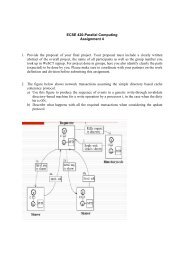
please see the notes at the end of this chapter. We begin with a program that prints
"Hello Universe!" on the screen, which is shown in a dissected form in Figure 1.1.
Figure 1.1: A "Hello Universe!" program.
16

The main "actors" in a Java program are objects. Objects store data and provide
methods for accessing and modifying this data. Every object is an instance of a class,
which defines the type of the object, as well as the kinds of operations that it
performs. The critical members of a class in Java are the following (classes can also
contain inner class definitions, but let us defer discussing this concept for now):
• Data of Java objects are stored in instance variables (also called fields).
Therefore, if an object from some class is to store data, its class must specify the
instance variables for such objects. Instance variables can either come from base
types (such as integers, floating-point numbers, or Booleans) or they can refer to
objects of other classes.
• The operations that can act on data, expressing the "messages" objects respond to,
are called methods, and these consist of constructors, procedures, and functions.
They define the behavior of objects from that class.
How Classes Are Declared
In short, an object is a specific combination of data and the methods that can
process and communicate that data. Classes define the types for objects; hence,
objects are sometimes referred to as instances of their defining class, because they
take on the name of that class as their type.
An example definition of a Java class is shown in Code Fragment 1.1.
Code Fragment 1.1: A Counter class for a simple
counter, which can be accessed, incremented, and
decremented.
17

In this example, notice that the class definition is delimited by braces, that is, it
begins with a "{" and ends with a "} ". In Java, any set of statements between the
braces "{" and "}" define a program block.
As with the Universe class, the Counter class is public, which means that any other
class can create and use a Counter object. The Counter has one instance variable—
an integer called count. This variable is initialized to 0 in the constructor method,
Counter, which is called when we wish to create a new Counter object (this method
always has the same name as the class it belongs to). This class also has one
accessor method, getCount, which returns the current value of the counter. Finally,
this class has two update methods—a method, incrementCount, which increments
the counter, and a method, decrementCount, which decrements the counter.
Admittedly, this is a pretty boring class, but at least it shows us the syntax and
structure of a Java class. It also shows us that a Java class does not have to have a
main method (but such a class can do nothing by itself).
The name of a class, method, or variable in Java is called an identifier, which can be
any string of characters as long as it begins with a letter and consists of letters,
numbers, and underscore characters (where "letter" and "number" can be from any
written language defined in the Unicode character set). We list the exceptions to
this general rule for Java identifiers in Table 1.1.
Table 1.1: A listing of the reserved words in Java.
These names cannot be used as method or variable
names in Java.
Reserved Words
abstract
18

else
interface
switch
boolean
extends
long
synchronized
break
false
native
this
byte
final
new
throw
case
finally
null
throws
catch
float
package
transient
char
for
19

private
true
class
goto
protected
try
const
if
public
void
continue
implements
return
volatile
default
import
short
while
do
instanceof
static
double
int
super
Class Modifiers
20

Class modifiers are optional keywords that precede the class keyword. We have
already seen examples that use the public keyword. In general, the different class
modifiers and their meaning is as follows:
• The abstract class modifier describes a class that has abstract methods.
Abstract methods are declared with the abstract keyword and are empty (that
is, they have no block defining a body of code for this method). A class that has
nothing but abstract methods and no instance variables is more properly called an
interface (see Section 2.4), so an abstract class usually has a mixture of
abstract methods and actual methods. (We discuss abstract classes and their uses
in Section 2.4.)
• The final class modifier describes a class that can have no subclasses.
(We will discuss this concept in the next chapter.)
• The public class modifier describes a class that can be instantiated or
extended by anything in the same package or by anything that imports the
class. (This is explained in more detail in Section 1.8.) Public classes are declared
in their own separate file called classname. java, where "classname" is the
name of the class.
• If the public class modifier is not used, the class is considered friendly.
This means that it can be used and instantiated by all classes in the same package.
This is the default class modifier.
1.1.1 Base Types
The types of objects are determined by the class they come from. For the sake of
efficiency and simplicity, Java also has the following base types (also called
primitive types), which are not objects:
boolean
Boolean value: true or false
char
16-bit Unicode character
byte
8-bit signed two's complement integer
short
16-bit signed two's complement integer
21

int
32-bit signed two's complement integer
long
64-bit signed two's complement integer
float
32-bit floating-point number (IEEE 754-1985)
double
64-bit floating-point number (IEEE 754-1985)
A variable declared to have one of these types simply stores a value of that type,
rather than a reference to some object. Integer constants, like 14 or 195, are of type
int, unless followed immediately by an 'L' or 'l', in which case they are of type long.
Floating-point constants, like 3.1415 or 2.158e5, are of type double, unless
followed immediately by an 'F' or 'f', in which case they are of type float. We show
a simple class in Code Fragment 1.2 that defines a number of base types as local
variables for the main method.
Code Fragment 1.2: A Base class showing
example uses of base types.
22

Comments
Note the use of comments in this and other examples. These comments are
annotations provided for human readers and are not processed by a Java compiler.
Java allows for two kinds of comments-block comments and inline commentswhich
define text ignored by the compiler. Java uses a /* to begin a block
comment and a */ to close it. Of particular note is a comment that begins with /**,
for such comments have a special format that allows a program called Javadoc to
read these comments and automatically generate documentation for Java
programs. We discuss the syntax and interpretation of Javadoc comments in
Section 1.9.3.
In addition to block comments, Java uses a // to begin inline comments and
ignores everything else on the line. All comments shown in this book will be
colored blue, so that they are not confused with executable code. For example:
/*
* This is a block comment.
*/
23

Output from the Base Class
// This is an inline comment.
Output from an execution of the Base class (main method) is shown in Figure 1.2.
Figure 1.2: Output from the Base class.
Even though they themselves do not refer to objects, base-type variables are
useful in the context of objects, for they often make up the instance variables (or
fields) inside an object. For example, the Counter class (Code Fragment 1.1) had a
single instance variable that was of type int. Another nice feature of base types in
Java is that base-type instance variables are always given an initial value when an
object containing them is created (either zero, false, or a null character, depending
on the type).
1.1.2 Objects
In Java, a new object is created from a defined class by using the new operator. The
new operator creates a new object from a specified class and returns a reference to
that object. In order to create a new object of a certain type, we must immediately
follow our use of the new operator by a call to a constructor for that type of object.
We can use any constructor that is included in the class definition, including the
default constructor (which has no arguments between the parentheses). In Figure
1.3, we show a number of dissected example uses of the new operator, both to
simply create new objects and to assign the reference to these objects to a variable.
Figure 1.3: Example uses of the new operator.
24

Calling the new operator on a class type causes three events to occur:
• A new object is dynamically allocated in memory, and all instance
variables are initialized to standard default values. The default values are null
for object variables and 0 for all base types except boolean variables (which are
false by default).
• The constructor for the new object is called with the parameters specified.
The constructor fills in meaningful values for the instance variables and performs
any additional computations that must be done to create this object.
• After the constructor returns, the new operator returns a reference (that is,
a memory address) to the newly created object. If the expression is in the form of
an assignment statement, then this address is stored in the object variable, so the
object variable refers to this newly created object.
Number Objects
We sometimes want to store numbers as objects, but base type numbers are not
themselves objects, as we have noted. To get around this obstacle, Java defines a
wrapper class for each numeric base type. We call these classes number classes.
In Table 1.2, we show the numeric base types and their corresponding number
class, along with examples of how number objects are created and accessed. Since
Java 5.0, a creation operation is performed automatically any time we pass a base
number to a method expecting a corresponding object. Likewise, the
25

corresponding access method is performed automatically any time we wish to
assign the value of a corresponding Number object to a base number type.
Table 1.2: Java number classes. Each class is given
with its corresponding base type and example
expressions for creating and accessing such objects.
For each row, we assume the variable n is declared
with the corresponding class name.
Base Type
Class Name
Creation Example
Access Example
byte
Byte
n = new Byte((byte)34);
n.byteValue( )
short
Short
n = new Short((short)100);
n.shortValue( )
int
Integer
n = new Integer(1045);
n.intValue( )
long
Long
n = new Long(10849L);
26

n.longValue( )
float
Float
n = new Float(3.934F);
n.floatValue( )
double
Double
n = new Double(3.934);
n.doubleValue( )
String Objects
A string is a sequence of characters that comes from some alphabet (the set of all
possible characters). Each character c that makes up a string s can be referenced
by its index in the string, which is equal to the number of characters that come
before c in s (so the first character is at index 0). In Java, the alphabet used to
define strings is the Unicode international character set, a 16-bit character
encoding that covers most used written languages. Other programming languages
tend to use the smaller ASCII character set (which is a proper subset of the
Unicode alphabet based on a 7-bit encoding). In addition, Java defines a special
built-in class of objects called String objects.
For example, a string P could be
"hogs and dogs",
which has length 13 and could have come from someone's Web page. In this case,
the character at index 2 is 'g' and the character at index 5 is 'a'. Alternately, P
could be the string "CGTAATAGTTAATCCG", which has length 16 and could
have come from a scientific application for DNA sequencing, where the alphabet
is {G, C, A, T}.
Concatenation
String processing involves dealing with strings. The primary operation for
combining strings is called concatenation, which takes a string P and a string Q
combines them into a new string, denoted P + Q, which consists of all the
characters of P followed by all the characters of Q. In Java, the "+" operation
27

works exactly like this when acting on two strings. Thus, it is legal (and even
useful) in Java to write an assignment statement like
Strings = "kilo" + "meters";
This statement defines a variable s that references objects of the String class,
and assigns it the string "kilometers". (We will discuss assignment statements
and expressions such as that above in more detail later in this chapter.) Every
object in Java is assumed to have a built-in method toString() that returns a
string associated with the object. This description of the String class should be
sufficient for most uses. We discuss the String class and its "relative" the
StringBuffer class in more detail in Section 12.1.
Object References
As mentioned above, creating a new object involves the use of the new operator
to allocate the object's memory space and use the object's constructor to initialize
this space. The location, or address, of this space is then typically assigned to a
reference variable. Therefore, a reference variable can be viewed as a "pointer" to
some object. It is as if the variable is a holder for a remote control that can be
used to control the newly created object (the device). That is, the variable has a
way of pointing at the object and asking it to do things or give us access to its
data. We illustrate this concept in Figure 1.4.
Figure 1.4: Illustrating the relationship between
objects and object reference variables. When we
assign an object reference (that is, memory address) to
a reference variable, it is as if we are storing that
object's remote control at that variable.
28

The Dot Operator
Every object reference variable must refer to some object, unless it is null, in
which case it points to nothing. Using the remote control analogy, a null reference
is a remote control holder that is empty. Initially, unless we assign an object
variable to point to something, it is null.
There can, in fact, be many references to the same object, and each reference to a
specific object can be used to call methods on that object. Such a situation would
correspond to our having many remote controls that all work on the same device.
Any of the remotes can be used to make a change to the device (like changing a
channel on a television). Note that if one remote control is used to change the
device, then the (single) object pointed to by all the remotes changes. Likewise, if
we use one object reference variable to change the state of the object, then its state
changes for all the references to it. This behavior comes from the fact that there
are many references, but they all point to the same object.
One of the primary uses of an object reference variable is to access the members
of the class for this object, an instance of its class. That is, an object reference
variable is useful for accessing the methods and instance variables associated with
an object. This access is performed with the dot (".") operator. We call a method
associated with an object by using the reference variable name, following that by
the dot operator and then the method name and its parameters.
This calls the method with the specified name for the object referred to by this
object reference. It can optionally be passed multiple parameters. If there are
several methods with this same name defined for this object, then the Java
runtime system uses the one that matches the number of parameters and most
closely matches their respective types. A method's name combined with the
number and types of its parameters is called a method's signature, for it takes all
29

of these parts to determine the actual method to perform for a certain method call.
Consider the following examples:
oven.cookDinner();
oven.cookDinner(food);
oven.cookDinner(food, seasoning);
Each of these method calls is actually referring to a different method with the
same name defined in the class that oven belongs to. Note, however, that the
signature of a method in Java does not include the type that the method returns, so
Java does not allow two methods with the same signature to return different types.
Instance Variables
Java classes can define instance variables, which are also called fields. These
variables represent the data associated with the objects of a class. Instance
variables must have a type, which can either be a base type (such as int,
float, double) or a reference type (as in our remote control analogy), that
is, a class, such as String an interface (see Section 2.4), or an array (see Section
1.5). A base-type instance variable stores the value of that base type, whereas an
instance variable declared with a class name stores a reference to an object of that
class.
Continuing our analogy of visualizing object references as remote controls,
instance variables are like device parameters that can be read or set from the
remote control (such as the volume and channel controls on a television remote
control). Given a reference variable v, which points to some object o, we can
access any of the instance variables for o that the access rules allow. For example,
public instance variables are accessible by everyone. Using the dot operator we
can get the value of any such instance variable, i, just by using v.i in an arithmetic
expression. Likewise, we can set the value of any such instance variable,i, by
writing v.i on the left-hand side of the assignment operator ("="). (See Figure 1.5.)
For example, if gnome refers to a Gnome object that has public instance variables
name and age, then the following statements are allowed:
gnome.name = "Professor Smythe";
gnome.age = 132;
Also, an object reference does not have to only be a reference variable. It can also
be any expression that returns an object reference.
Figure 1.5: Illustrating the way an object reference
can be used to get and set instance variables in an
30

object (assuming we are allowed access to those
variables).
Variable Modifiers
In some cases, we may not be allowed to directly access some of the instance
variables for an object. For example, an instance variable declared as private in
some class is only accessible by the methods defined inside that class. Such
instance variables are similar to device parameters that cannot be accessed
directly from a remote control. For example, some devices have internal
parameters that can only be read or assigned by a factory technician (and a user is
not allowed to change those parameters without violating the device's warranty).
When we declare an instance variable, we can optionally define such a variable
modifier, follow that by the variable's type and the identifier we are going to use
for that variable. Additionally, we can optionally assign an initial value to the
variable (using the assignment operator ("="). The rules for a variable name are
the same as any other Java identifier. The variable type parameter can be either a
base type, indicating that this variable stores values of this type, or a class name,
indicating that this variable is a reference to an object from this class. Finally, the
optional initial value we might assign to an instance variable must match the
variable's type. For example, we could define a Gnome class, which contains
several definitions of instance variables, shown in in Code Fragment 1.3.
31

The scope (or visibility) of instance variables can be controlled through the use of
the following variable modifiers:
• public: Anyone can access public instance variables.
• protected: Only methods of the same package or of its subclasses can
access protected instance variables.
• private: Only methods of the same class (not methods of a subclass) can
access private instance variables.
• If none of the above modifiers are used, the instance variable is considered
friendly. Friendly instance variables can be accessed by any class in the same
package. Packages are discussed in more detail in Section 1.8.
In addition to scope variable modifiers, there are also the following usage
modifiers:
• static: The static keyword is used to declare a variable that is associated
with the class, not with individual instances of that class. Static variables are
used to store "global" information about a class (for example, a static variable
could be used to maintain the total number of Gnome objects created). Static
variables exist even if no instance of their class is created.
• final: A final instance variable is one that must be assigned an initial
value, and then can never be assigned a new value after that. If it is a base type,
then it is a constant (like the MAX_HEIGHT constant in the Gnome class). If
an object variable is final, then it will always refer to the same object (even if
that object changes its internal state).
Code Fragment 1.3: The Gnome class.
32

Note the uses of instance variables in the Gnome example. The variables age,
magical, and height are base types, the variable name is a reference to an instance
of the built-in class String, and the variable gnomeBuddy is a reference to an
object of the class we are now defining. Our declaration of the instance variable
MAX_HEIGHT in the Gnome class is taking advantage of these two modifiers to
33

define a "variable" that has a fixed constant value. Indeed, constant values
associated with a class should always be declared to be both static and final.
1.1.3 Enum Types
Since 5.0, Java supports enumerated types, called enums. These are types that are
only allowed to take on values that come from a specified set of names. They are
declared inside of a class as follows:
modifier enum name { value_name 0 , value_name 1 , …,
value_name n−1 };
where the modifier can be blank, public, protected, or private. The name of this
enum, name, can be any legal Java identifier. Each of the value identifiers,
valuenamei, is the name of a possible value that variables of this enum type can
take on. Each of these name values can also be any legal Java identifier, but the
Java convention is that these should usually be capitalized words. For example, the
following enumerated type definition might be useful in a program that must deal
with dates:
};
public enum Day { MON, TUE, WED, THU, FRI, SAT, SUN
Once defined, we can use an enum type, such as this, to define other variables,
much like a class name. But since Java knows all the value names for an
enumerated type, if we use an enum type in a string expression, Java will
automatically use its name. Enum types also have a few built-in methods, including
a method valueOf, which returns the enum value that is the same as a given string.
We show an example use of an enum type in Code Fragment 1.4.
Code Fragment 1.4:
type.
An example use of an enum
34

1.2 Methods
Methods in Java are conceptually similar to functions and procedures in other
highlevel languages. In general, they are "chunks" of code that can be called on a
particular object (from some class). Methods can accept parameters as arguments, and
their behavior depends on the object they belong to and the values of any parameters
that are passed. Every method in Java is specified in the body of some class. A
method definition has two parts: the signature, which defines the and parameters for
a method, and the body, which defines what the method does.
A method allows a programmer to send a message to an object. The method signature
specifies how such a message should look and the method body specifies what the
object will do when it receives such a message.
Declaring Methods
The syntax for defining a method is as follows:
modifiers type name(type 0 parameter 0 , …, type n−1 parameter n−1 ) {
}
// method body …
35

Each of the pieces of this declaration have important uses, which we describe in
detail in this section. The modifiers part includes the same kinds of scope modifiers
that can be used for variables, such as public, protected, and static, with similar
meanings. The type part of the declaration defines the return type of the method.
The name is the name of the method, which can be any valid Java identifier. The
list of parameters and their types declares the local variables that correspond to the
values that are to be passed as arguments to this method. Each type declaration type i
can be any Java type name and each parameter i can be any Java identifier. This list
of parameters and their types can be empty, which signifies that there are no values
to be passed to this method when it is invoked. These parameter variables, as well
as the instance variables of the class, can be used inside the body of the method.
Likewise, other methods of this class can be called from inside the body of a
method.
When a method of a class is called, it is invoked on a specific instance of that class
and can change the state of that object (except for a static method, which is
associated with the class itself). For example, invoking the following method on
particular gnome changes its name.
public void renameGnome (String s) {
name = s; // Reassign the name instance variable
of this gnome.
}
Method Modifiers
As with instance variables, method modifiers can restrict the scope of a method:
• public: Anyone can call public methods.
• protected: Only methods of the same package or of subclasses can call a
protected method.
• private: Only methods of the same class (not methods of a subclass) can
call a private method.
• If none of the modifiers above are used, then the method is friendly.
Friendly methods can only be called by objects of classes in the same package.
The above modifiers may be preceded by additional modifiers:
• abstract: A method declared as abstract has no code. The signature of
such a method is followed by a semicolon with no method body. For example:
public abstract void setHeight (double newHeight);
36

Abstract methods may only appear within an abstract class. We discuss the
usefulness of this construct in Section 2.4.
• final: This is a method that cannot be overridden by a subclass.
• static: This is a method that is associated with the class itself, and not with
a particular instance of the class. Static methods can also be used to change the
state of static variables associated with a class (provided these variables are not
declared to be final).
Return Types
A method definition must specify the type of value the method will return. If the
method does not return a value, then the keyword void must be used. If the return
type is void, the method is called a procedure; otherwise, it is called a function. To
return a value in Java, a method must use the return keyword (and the type
returned must match the return type of the method). Here is an example of a method
(from inside the Gnome class) that is a function:
public booleanisMagical () {
}
returnmagical;
As soon as a return is performed in a Java function, the method ends.
Java functions can return only one value. To return multiple values in Java, we
should instead combine all the values we wish to return in a compound object,
whose instance variables include all the values we want to return, and then return a
reference to that compound object. In addition, we can change the internal state of
an object that is passed to a method as another way of "returning" multiple results.
Parameters
A method's parameters are defined in a comma-separated list enclosed in
parentheses after the name of the method. A parameter consists of two parts, the
parameter type and the parameter name. If a method has no parameters, then only
an empty pair of parentheses is used.
All parameters in Java are passed by value, that is, any time we pass a parameter to
a method, a copy of that parameter is made for use within the method body. So if
we pass an int variable to a method, then that variable's integer value is copied.
The method can change the copy but not the original. If we pass an object reference
as a parameter to a method, then the reference is copied as well. Remember that we
can have many different variables that all refer to the same object. Changing the
37

internal reference inside a method will not change the reference that was passed in.
For example, if we pass a Gnome reference g to a method that calls this parameter
h, then this method can change the reference h to point to a different object, but g
will still refer to the same object as before. Of course, the method can use the
reference h to change the internal state of the object, and this will change g's object
as well (since g and h are currently referring to the same object).
Constructors
A constructor is a special kind of method that is used to initialize newly created
objects. Java has a special way to declare the constructor and a special way to
invoke the constructor. First, let's look at the syntax for declaring a constructor:
modifiers name(type 0 parameter 0 , …, type n−1 parameter n−1 ) {
}
// constructor body …
Thus, its syntax is essentially the same as that of any other method, but there are
some important differences. The name of the constructor, name, must be the same
as the name of the class it constructs. So, if the class is called Fish, the constructor
must be called Fish as well. In addition, we don't specify a return type for a
constructor—its return type is implicitly the same as its name (which is also the
name of the class). Constructor modifiers, shown above as modifiers, follow the
same rules as normal methods, except that an abstract, static, or final
constructor is not allowed.
Here is an example:
publicFish (intw, String n) {
}
weight = w;
name = n,;
Constructor Definition and Invocation
The body of a constructor is like a normal method's body, with a couple of minor
exceptions. The first difference involves a concept known as constructor chaining,
which is a topic discussed in Section 2.2.3 and is not critical at this point.
The second difference between a constructor body and that of a regular method is
that return statements are not allowed in a constructor body. A constructor's body
38

is intended to be used to initialize the data associated with objects of this class so
that they may be in a stable initial state when first created.
Constructors are invoked in a unique way: they must be called using the new
operator. So, upon invocation, a new instance of this class is automatically created
and its constructor is then called to initialize its instance variables and perform other
setup tasks. For example, consider the following constructor invocation (which is
also a declaration for the myFish variable):
Fish myFish = new Fish (7, "Wally");
A class can have many constructors, but each must have a different signature, that
is, each must be distinguished by the type and number of the parameters it takes.
The main Method
Some Java classes are meant to be used by other classes, others are meant to be
stand-alone programs. Classes that define stand-alone programs must contain one
other special kind of method for a class—the main method. When we wish to
execute a stand-alone Java program, we reference the name of the class that defines
this program by issuing the following command (in a Windows, Linux, or UNIX
shell):
java Aquarium
In this case, the Java run-time system looks for a compiled version of the
Aquarium class, and then invokes the special main method in that class. This
method must be declared as follows:
public static voidmain(String[] args){
}
// main method body …
The arguments passed as the parameter args to the main method are the
commandline arguments given when the program is called. The args variable is an
array of String objects, that is, a collection of indexed strings, with the first string
being args[0], the second being args[1], and so on. (We say more about arrays in
Section 1.5.)
Calling a Java Program from the Command Line
Java programs can be called from the command line using the java command,
followed by the name of the Java class whose main method we wish to run, plus
39

any optional arguments. For example, we may have defined the Aquarium
program to take an optional argument that specifies the number of fish in the
aquarium. We could then invoke the program by typing the following in a shell
window:
java Aquarium 45
to specify that we want an aquarium with 45 fish in it. In this case, args[0] would
refer to the string "45". One nice feature of the main method in a class definition is
that it allows each class to define a stand-alone program, and one of the uses for this
method is to test all the other methods in a class. Thus, thorough use of the main
method is an effective tool for debugging collections of Java classes.
Statement Blocks and Local Variables
The body of a method is a statement block, which is a sequence of statements and
declarations to be performed between the braces "{" and "}". Method bodies and
other statement blocks can themselves have statement blocks nested inside of them.
In addition to statements that perform some action, like calling the method of some
object, statement blocks can contain declarations of local variables. These variables
are declared inside the statement body, usually at the beginning (but between the
braces "{" and "}"). Local variables are similar to instance variables, but they only
exist while the statement block is being executed. As soon as control flow exits out
of that block, all local variables inside it can no longer be referenced. A local
variable can either be a base type (such as int, float, double) or a
reference to an instance of some class. Single statements and declarations in Java
are always terminated by a semicolon, that is, a ";".
There are two ways of declaring local variables:
type name;
type name = initial_value;
The first declaration simply defines the identifier, name, to be of the specified type.
The second declaration defines the identifier, its type, and also initializes this
variable to the specified value. Here are some examples of local variable
declarations:
{
double r;
Point p1 = new Point (3, 4);
Point p2 = new Point (8, 2);
40

}
int i = 512;
double e = 2.71828;
1.3 Expressions
Variables and constants are used in expressions to define new values and to modify
variables. In this section, we discuss how expressions work in Java in more detail.
Expressions involve the use of literals, variables, and operators. Since we have
already discussed variables, let us briefly focus on literals and then discuss operators
in some detail.
1.3.1 Literals
A literal is any "constant" value that can be used in an assignment or other
expression. Java allows the following kinds of literals:
• The null object reference (this is the only object literal, and it is defined
to be from the general Object class).
• Boolean: true and false.
• Integer: The default for an integer like 176, or -52 is that it is of type int,
which is a 32-bit integer. A long integer literal must end with an "L" or "l," for
example, 176L or −52l, and defines a 64-bit integer.
• Floating Point: The default for floating- numbers, such as 3.1415 and
10035.23, is that they are double. To specify that a literal is a float, it must
end with an "F" or "f." Floating-point literals in exponential notation are also
allowed, such as 3.14E2 or .19e10; the base is assumed to be 10.
• Character: In Java, character constants are assumed to be taken from the
Unicode alphabet. Typically, a character is defined as an individual symbol
enclosed in single quotes. For example, 'a' and '?' are character constants. In
addition, Java defines the following special character constants:
'\n' (newline)
'\t' (tab)
'\b' (backspace)
'\r' (return)
41

'\f' (formfeed)
'\\' (backslash)
'\'' (single quote)
'\"' (double quote).
• String Lieral: A string literal is a sequence of characters enclosed in
double quotes, for example, the following is a string literal:
"dogs cannot climb trees"
1.3.2 Operators
Java expressions involve composing literals and variables with operators. We
survey the operators in Java in this section.
The Assignment Operator
The standard assignment operator in Java is "=". It is used to assign a value to an
instance variable or local variable. Its syntax is as follows:
variable = expression
where variable refers to a variable that is allowed to be referenced by the
statement block containing this expression. The value of an assignment operation
is the value of the expression that was assigned. Thus, if i and j are both
declared as type int, it is correct to have an assignment statement like the
following:
i = j = 25;// works because '=' operators are
evaluated right-to-left
Arithmetic Operators
The following are binary arithmetic operators in Java:
+ addition
− subtraction
* multiplication
/ division
42

% the modulo operator
This last operator, modulo, is also known as the "remainder" operator, because it
is the remainder left after an integer division. We often use "mod" to denote the
modulo operator, and we define it formally as
n mod m = r,
such that
n = mq + r,
for an integer q and 0 ≤ r < n.
Java also provides a unary minus (−), which can be placed in front of an arithm
etic expression to invert its sign. Parentheses can be used in any expression to
define the order of evaluation. Java also uses a fairly intuitive operator precedence
rule to determine the order of evaluation when parentheses are not used. Unlike
C++, Java does not allow operator overloading.
Increment and Decrement Operators
Like C and C++, Java provides increment and decrement operators. Specifically,
it provides the plus-one increment (++) and decrement (−−) operators. If such an
operator is used in front of a variable reference, then 1 is added to (or subtracted
from) the variable and its value is read into the expression. If it is used after a
variable reference, then the value is first read and then the variable is incremented
or decremented by 1. So, for example, the code fragment
int i = 8;
int j = i++;
int k = ++i;
int m = i−−;
int n = 9 + i++;
assigns 8 to j, 10 to k, 10 to m, 18 to n, and leaves i with value 10.
Logical Operators
Java allows for the standard comparison operators between numbers:
< less than
43

= greater than or equal
> greater than
The operators == and != can also be used for object references. The type of the
result of a comparison is a boolean.
Operators that operate on boolean values are the following:
! not (prefix)
&&
conditional and
conditional or
The Boolean operators && and will not evaluate the second operand (to the
right) in their expression if it is not needed to determine the value of the
expression. This feature is useful, for example, for constructing Boolean
expressions where we first test that a certain condition holds (such as a reference
not being null), and then test a condition that could have otherwise generated an
error condition had the prior test not succeeded.
Bitwise Operators
Java also provides the following bitwise operators for integers and Booleans:
operator)
bitwise complement (prefix unary
& bitwise and
| bitwise or
^ bitwise exclusive-or
< < shift bits left, filling in with zeros
bit
> > shift bits right, filling in with sign
44

zeros
>>> shift bits right, filling in with
Operational Assignment Operators
Besides the standard assignment operator (=), Java also provides a number of
other assignment operators that have operational side effects. These other kinds of
operators are of the following form:
variable op = expression
where op is any binary operator. The above expression is equivalent to
variable = variable op expression
except that if variable contains an expression (for example, an array index),
the expression is evaluated only once. Thus, the code fragment
a [5] = 10;
i = 5;
a[i++] += 2;
leaves a [5] with value 12 and i with value 6.
String Concatenation
Strings can be composed using the concatenation operator (+), so that the code
String rug = "carpet";
String dog = "spot";
String mess = rug + dog;
String answer = mess + " will cost me " + 5 + "
dollars!";
would have the effect of making answer refer to the string
"carpetspot will cost me 5 dollars!"
This example also shows how Java converts nonstring constants into strings,
when they are involved in a string concatenation operation.
45

Operator Precedence
Operators in Java are given preferences, or precedence, that determine the order in
which operations are performed when the absence of parentheses brings up
evaluation ambiguities. For example, we need a way of deciding if the expression,
"5+2*3," has value 21 or 11 (Java says it is 11).
We show the precedence of the operators in Java (which, incidentally, is the same
as in C) in Table 1.3.
Table 1.3: The Java precedence rules. Operators in
Java are evaluated according to the above ordering, if
parentheses are not used to determine the order of
evaluation. Operators on the same line are evaluated
in left-to-right order (except for assignment and prefix
operations, which are evaluated right-to-left), subject
to the conditional evaluation rule for Boolean and and
or operations. The operations are listed from highest
to lowest precedence (we use exp to denote an atomic
or parenthesized expression). Without
parenthesization, higher precedence operators are
performed before lower precedence operators.
Operator Precedence
Type
Symbols
1
postfix ops prefix ops cast
exp ++ exp −− ++exp −−exp +exp −exp ∼exp !exp (type) exp
2
mult./div.
* / %
46

3
add./subt.
+ −
4
shift
> >>>
5
comparison
< >= instanceof
6
equality
== !=
7
bitwise-and
&
8
bitwise-xor
^
9
bitwise-or
|
10
and
&&
11
47

or
12
conditional
boolean_expression? value_if_true:
value_if_false
13
assignment
= += −= *= /= %= >>= >=&= ^= | =
We have now discussed almost all of the operators listed in Table 1.3. A notable
exception is the conditional operator, which involves evaluating a Boolean
expression and then taking on the appropriate value depending on whether this
Boolean expression is true or false. (We discuss the use of the instanceof
operator in the next chapter.)
1.3.3 Casting and Autoboxing/Unboxing in Expressions
Casting is an operation that allows us to change the type of a variable. In essence,
we can take a variable of one type and cast it into an equivalent variable of another
type. Casting can be useful for doing certain numerical and input/output operations.
The syntax for casting an expression to a desired type is as follows:
(type) exp
where type is the type that we would like the expression exp to have. There are two
fundamental types of casting that can be done in Java. We can either cast with
respect to the base numerical types or we can cast with respect to objects. here, we
discuss how to perform casting of numerical and string types, and we discuss object
casting in Section 2.5.1. For instance, it might be helpful to cast an int to a
double in order to perform operations like division.
Ordinary Casting
When casting from a double to an int, we may lose precision. This means that
the resulting double value will be rounded down. But we can cast an int to a
double without this worry. For example, consider the following:
48

double d1 = 3.2;
double d2 = 3.9999;
int i1 = (int)d1; // i1 has value 3
int i2 = (int)d2; // i2 has value 3
double d3 = (double)i2; // d3 has value 3.0
Casting with Operators
Certain binary operators, like division, will have different results depending on
the variable types they are used with. We must take care to make sure operations
perform their computations on values of the intended type. When used with
integers, division does not keep track of the fractional part, for example. When
used with doubles, division keeps this part, as is illustrated in the following
example:
int i1 = 3;
int i2 = 6;
dresult = (double)i1 / (double)i2;// dresult has
value 0.5
dresult = i1 / i2;
value 0.0
// dresult has
Notice that when i1 and i2 were cast to doubles, regular division for real
numbers was performed. When i1 and i2 were not cast, the " /" operator
performed an integer division and the result of i1 / i2 was the int 0. Then,
JavaJava then did an implicit cast to assign an int value to the double result.
We discuss implicit casting next.
Implicit Casting and Autoboxing/Unboxing
There are cases where Java will perform an implicit cast, according to the type of
the assignment variable, provided there is no loss of precision. For example:
int iresult, i = 3;
double dresult, d = 3.2;
dresult = i / d;
cast to a double
// dresult is 0.9375. i was
49

iresult = i / d; // loss of precision −>
this is a compilation error
iresult = (int) i / d;
fractional part is lost
// iresult is 0, since the
Note that since Java will not perform implicit casts where precision is lost, the
explicit cast in the last line above is required.
Since Java 5.0, there is a new kind of implicit cast, for going between Number
objects, like Integer and Float, and their related base types, like int and
float. Any time a Number object is expected as a parameter to a method, the
corresponding base type can be passed. In this case, Java will perform an implicit
cast, called autoboxing, which will convert the base type to its corresponding
Number object. Likewise, any time a base type is expected in an expression
involving a Number reference, that Number object is changed to the
corresponding base type, in an operation called unboxing.
There are few caveats regarding autoboxing and unboxing, however. One is that if
a Number reference is null, then trying to unbox it will generate an error, called
NullPointerException. Second, the operator, "==", is used both to test the
equality of base type values as well as whether two Number references are
pointing to the same object. So when testing for equality, try to avoid the implicit
casts done by autoboxing and unboxing. Finally, implicit casts, of any kind, take
time, so we should try to minimize our reliance on them if performance is an
issue.
Incidentally, there is one situation in Java when only implicit casting is allowed,
and that is in string concatenation. Any time a string is concatenated with any
object or base type, that object or base type is automatically converted to a string.
Explicit casting of an object or base type to a string is not allowed, however.
Thus, the following assignments are incorrect:
String s = (String) 4.5; ;
wrong!
// this is
String t = "Value = " + (String) 13;// this is
wrong!
String u = 22;
// this is wrong!
To perform a conversion to a string, we must instead use the appropriate
toString method or perform an implicit cast via the concatenation operation.
Thus, the following statements are correct:
50

String s = " " + 4.5; // correct, but
poor style
String t = "Value = " + 13;
String u = Integer.toString(22);
good
// this is good
// this is
1.4 Control Flow
Control flow in Java is similar to that of other high-level languages. We review the
basic structure and syntax of control flow in Java in this section, including method
returns, if statements, switch statements, loops, and restricted forms of "jumps"
(the break and continue statements).
1.4.1 The If and Switch Statements
In Java, conditionals work similarly to the way they work in other languages. They
provide a way to make a decision and then execute one or more different statement
blocks based on the outcome of that decision.
The If Statement
The syntax of a simple if statement is as follows:
if (boolean_exp)
else
true_statement
false_statement
where boolean_exp is a Boolean expression and true_statement and
false_statement are each either a single statment or a block of statements enclosed
in braces ("{" and "}"). Note that, unlike some similar languages, the value tested
by an if statement in Java must be a Boolean expression. In particular, it is
definitely not an integer expression. Nevertheless, as in other similar languages,
the else part (and its associated statement) in a Java if statement is optional.
There is also a way to group a number of Boolean tests, as follows:
if (first_boolean_exp)
true_statement
51

else if (second_boolean_exp)
else
second_true_statement
false_statement
If the first Boolean expression is false, the second Boolean expression will be
tested, and so on. An if statement can have an arbitrary number of else if
parts.
For example, the following is a correct if statement.
if (snowLevel < 2) {
}
goToClass();
comeHome();
else if (snowLevel < 5) {
}
else
goSledding();
haveSnowballFight();
stayAtHome();
Switch Statements
Java provides for multiple-value control flow using the switch statement, which is
especially useful with enum types. The following is an indicative example (based
on a variable d of the Day enum type of Section 1.1.3).
switch (d) {
case MON:
52

System.out.println("This is tough.");
break;
case TUE:
System.out.println("This is getting better.");
break;
case WED:
System.out.println("Half way there.");
break;
case THU:
System.out.println("I can see the light.");
break;
case FRI:
System.out.println("Now we are talking.");
break;
default:
System.out.println("Day off ! ");
break;
}
The switch statement evaluates an integer or enum expression and causes
control flow to jump to the code location labeled with the value of this expression.
If there is no matching label, then control flow jumps to the location labeled
"default." This is the only explicit jump performed by the switch
statement, however, so flow of control "falls through" to other cases if the code
for each case is not ended with a break statement (which causes control flow to
jump to the next line after the switch statement).
1.4.2 Loops
53

Another important control flow mechanism in a programming language is looping.
Java provides for three types of loops.
While Loops
The simplest kind of loop in Java is a while loop. Such a loop tests that a certain
condition is satisfied and will perform the body of the loop each time this
condition is evaluated to be true. The syntax for such a conditional test before a
loop body is executed is as follows:
while (boolean_exp)
loop_statement
At the beginning of each iteration, the loop tests the expression, boolean exp, and
then executes the loop body, loop_statement, only if this Boolean expression
evaluates to true. The loop body statement can also be a block of statements.
Consider, for example, a gnome that is trying to water all of the carrots in his
carrot patch, which he does as long as his watering can is not empty. Since his can
might be empty to begin with, we would write the code to perform this task as
follows:
public void waterCarrots () {
}
Carrot current = garden.findNextCarrot ();
while (!waterCan.isEmpty ()) {
}
water (current, waterCan);
current = garden.findNextCarrot ();
Recall that "!" in Java is the "not" operator.
For Loops
Another kind of loop is thefor loop. In their simplest form, for loops provide
for repeated code based on an integer index. In Java, we can do that and much
more. The functionality of a for loop is significantly more flexible. In particular,
the usage of a for loop is split into four sections: the initialization, the condition,
the increment, and the body.
54

Defining a For Loop
Here is the syntax for a Java for loop:
for (initialization; condition; increment)
loop_statement
where each of the sections initialization, condition, and increment can be empty.
In the initialization section, we can declare an index variable that will only exist
in the scope of the for loop. For example, if we want a loop that indexes on a
counter, and we have no need for the counter variable outside of the for loop,
then declaring something like the following
for (int counter = 0; condition; increment)
loop_statement
will declare a variable counter whose scope is the loop body only.
In the condition section, we specify the repeat (while) condition of the loop. This
must be a Boolean expression. The body of the for loop will be executed each
time the condition is true when evaluated at the beginning of a potential
iteration. As soon as condition evaluates to false, then the loop body is not
executed, and, instead, the program executes the next statement after the for
loop.
In the increment section, we declare the incrementing statement for the loop. The
incrementing statement can be any legal statement, allowing for significant
flexibility in coding. Thus, the syntax of a for loop is equivalent to the
following:
initialization;
while (condition) {
}
loop_statement;
increment;
except that, in Java, a while loop cannot have an empty Boolean condition,
whereas a for loop can. The following example shows a simple for loop in
Java:
55

public void eatApples (Apples apples) {
}
numApples = apples.getNumApples ();
for (int x = 0; × < numApples; ×++) {
}
eatApple (apples.getApple (×));
spitOutCore ();
In the Java example above, the loop variable x was declared as int x = 0.
Before each iteration, the loop tests the condition " x < numApples" and
executes the loop body only if this is true. Finally, at the end of each iteration the
loop uses the statement x++ to increment the loop variable x before again testing
the condition.
Incidentally, since 5.0, Java also includes a for-each loop, which we discuss in
Section 6.3.2.
Do-While Loops
Java has yet another kind of loop besides the for loop and the standard while
loop—the do-while loop. The former loops tests a condition before performing
an iteration of the loop body, the do-while loop tests a condition after the loop
body. The syntax for a do-while loop is as shown below:
do
loop_statement
while (boolean_exp)
Again, the loop body statement, loop_statement, can be a single statement or a
block of statements, and the conditional, boolean_exp, must be a Boolean
expression. In a do-while loop, we repeat the loop body for as long as the
condition is true each time it is evaluated.
Consider, for example, that we want to prompt the user for input and then do
something useful with that input. (We discuss Java input and output in more detail
in Section 1.6.) A possible condition, in this case, for exiting the loop is when the
user enters an empty string. However, even in this case, we may want to handle
56

that input and inform the user that he or she has quit. The following example
illustrates this case:
public void getUserInput() {
}
String input;
do {
input = getInputString();
handleInput(input);
} while (input.length()>0);
Notice the exit condition for the above example. Specifically, it is written to be
consistent with the rule in Java that do-while loops exit when the condition is
not true (unlike the repeat-until construct used in other languages).
1.4.3 Explicit Control-Flow Statements
Java also provides statements that allow for explicit change in the flow of control of
a program.
Returning from a Method
If a Java method is declared with a return type of void, then flow of control
returns when it reaches the last line of code in the method or when it encounters a
return statement with no argument. If a method is declared with a return type,
however, the method is a function and it must exit by returning the function's
value as an argument to a return statement. The following (correct) example
illustrates returning from a function:
// Check for a specific birthday
public boolean checkBDay (int date) {
if (date == Birthdays.MIKES_BDAY) {
}
return true;
return false;
57

}
It follows that the return statement must be the last statement executed in a
function, as the rest of the code will never be reached.
Note that there is a significant difference between a statement being the last line
of code that is executed in a method and the last line of code in the method itself.
In the example above, the line return true; is clearly not the last line of code
that is written in the function, but it may be the last line that is executed (if the
condition involving date is true). Such a statement explicitly interrupts the flow
of control in the method. There are two other such explicit control-flow
statements, which are used in conjunction with loops and switch statements.
The break Statement
The typical use of a break statement has the following simple syntax:
break;
It is used to "break" out of the innermost switch, for, while, or dowhile
statement body. When it is executed, a break statement causes the flow of
control to jump to the next line after the loop or switch to the body containing
the break.
The break statement can also be used in a labeled form to jump out of an
outernested loop or switch statement. In this case, it has the syntax
break label;
where label is a Java identifier that is used to label a loop or switch statement.
Such a label can only appear at the beginning of the declaration of a loop. There
are no other kinds of "go to" statements in Java.
We illustrate the use of a label with a break statement in the following simple
example:
public static boolean hasZeroEntry (int[][] a) {
boolean foundFlag = false;
zeroSearch:
for (int i=0; i

if (a[i][j] == 0) {
foundFlag = true;
break zeroSearch;
}
}
}
}
return foundFlag;
The example above also uses arrays, which are covered in Section 3.1.
The continue Statement
The other statement to explicitly change the flow of control in a Java program is
the continue statement, which has the following syntax:
continue label;
where label is an optional Java identifier that is used to label a loop. As
mentioned above, there are no explicit "go to" statements in Java. Likewise, the
continue statement can only be used inside loops (for, while, and dowhile).
The continue statement causes the execution to skip over the
remaining steps of the loop body in the current iteration (but then continue the
loop if its condition is satisfied).
1.5 Arrays
A common programming task is to keep track of a numbered group of related objects.
For example, we may want a video game to keep track of the top ten scores for that
game. Rather than use ten different variables for this task, we would prefer to use a
single name for the group and use index numbers to refer to the high scores in that
group. Similarly, we may want a medical information system to keep track of the
patients currently assigned to beds in a certain hospital. Again, we would rather not
have to introduce 200 variables in our program just because the hospital has 200 beds.
In such cases, we can save programming effort by using an array, which is a
numbered collection of variables all of the same type. Each variable, or cell, in an
array has an index, which uniquely refers to the value stored in that cell. The cells of
59

an array a are numbered 0, 1,2, and so on. We illustrate an array of high scores for a
video game in Figure 1.6.
Figure 1.6: An illustration of an array of ten (int) high
scores for a video game.
Such an organization is quite useful, for it allows us to do some interesting
computations. For example, the following method adds up all the numbers in an array
of integers:
/** Adds all the numbers in an integer array. */
public static int sum(int[] a) {
int total = 0;
for (int i=0; i < a.length; i==) // note the use of the length
variable
total += a[i];
return total;
}
This example takes advantage of a nice feature of Java, which allows us to find the
number of cells an array stores, that is, its length. In Java, an array a is a special kind
of object and the length of a is stored in an instance variable, length. That is, we
never need to guess the length of an array in Java, the length of an array can be
accessed as follows:
array_name.length
where array_name is the name of the array. Thus, the cells of an array a are
numbered 0, 1,2, and so on, up to a.length − 1.
Array Elements and Capacities
Each object stored in an array is called an element of that array. Element number 0
is a[0], element number 1 is a[1], element number 2 is a[2], and so on. Since the
length of an array determines the maximum number of things that can be stored in
60

the array, we will sometimes refer to the length of an array as its capacity. We show
another simple use of an array in the following code fragment, which counts the
number of times a certain number appears in an array:
/** Counts the number of times an integer appears in
an array. */
public static int findCount(int[] a, int k) {
int count = 0;
for (int e: a) {
// note the use of the "foreach" loop
}
if (e == k) // check if the current element equals k
count++;
return count;
}
Out of Bounds Errors
It is a dangerous mistake to attempt to index into an array a using a number outside
the range from 0 to a.length &minus; 1. Such a reference is said to be out of
bounds. Out of bounds references have been exploited numerous times by hackers
using a method called the buffer overflow attack to compromise the security of
computer systems written in languages other than Java. As a safety feature, array
indices are always checked in Java to see if they are ever out of bounds. If an array
index is out of bounds, the run-time Java environment signals an error condition.
The name of this condition is the ArrayIndexOutOfBoundsException. This
check helps Java avoid a number of security problems (including buffer overflow
attacks) that other languages must cope with.
We can avoid out-of-bounds errors by making sure that we alway index into an
array, a, using an integer value between 0 and a.length. One shorthand way we
can do this is by carefully using the early termination feature of Boolean operations
in Java. For example, a statement like the following will never generate an index
out-of-bounds error:
if ((i >= 0) && (i < a.length) && (a[i] > 2) )
× = a[i];
61

for the comparison "a[i] > 0.5" will only be performed if the first two
comparisons succeed.
1.5.1 Declaring Arrays
One way to declare and initialize an array is as follows:
element_type[] array_name = {init_val_0,init_val_1,…,init_val_N−1};
The element_type can be any Java base type or class name, and array_name can be
any value Java identifier. The initial values must be of the same type as the array.
For example, consider the following declaration of an array that is initialized to
contain the first ten prime numbers:
int[] primes = {2, 3, 5, 7, 11, 13, 17, 19, 23, 29};
In addition to creating an array and defining all its initial values when we declare it,
we can declare an array variable without initializing it. The form of this declaration
is as follows:
element_type[] array_name;
An array created in this way is initialized with all zeros if the array type is a number
type. Arrays of objects are initialized to all null references. Once we have
declared an array in this way, we can create the collection of cells for an array later
using the following syntax:
new element_type[length]
where length is a positive integer denoting the length of the array created. Typically
this expression appears in an assignment statement with an array name on the left
hand side of the assignment operator. So, for example, the following statement
defines an array variable named a, and later assigns it an array of 10 cells, each of
type double, which it then initializes:
double[] a;
//… various steps …
a = new double[10];
for (int k=0; k < a.length; k++) {
}
a[k] = 1.0;
62

The cells of this new array, "a," are indexed using the integer set {0,1,2,… ,9}
(recall that arrays in Java always start indexing at 0), and, like every array in Java,
all the cells in this array are of the same type—double.
1.5.2 Arrays are Objects
Arrays in Java are special kinds of objects. In fact, this is the reason we can use the
new operator to create a new instance of an array. An array can be used just like
any general object in Java, but we have a special syntax (using square brackets, "["
and "]") to refer to its members. An array in Java can do everything that a general
object can. Since an array is an object, though, the name of an array in Java is
actually a reference to the place in memory where the array is stored. Thus, there is
nothing too special about using the dot operator and the instance variable, length, to
refer to the length of an array, for example, as "a.length." The name, a, in this
case is just a reference, or pointer, to the underlying array object.
The fact that arrays in Java are objects has an important implication when it comes
to using array names in assignment statements. For when we write something like
b = a;
in a Java program, we really mean that b and a now both refer to the same array.
So, if we then write something like
b[3] = 5;
then we will also be setting the number a [3] to 5. We illustrate this crucial point in
Figure 1.7.
Figure 1.7: An illustration of an assignment of array
objects. We show the result of setting "b[3] = 5;"
after previously setting "b = a;".
63

Cloning an Array
If instead, we wanted to create an exact copy of the array, a, and assign that array
to the array variable, b, we should write
b = a.clone();
which copies all of the cells of a into a new array and assigns b to point to that
new array. In fact, the clone method is a built-in method of every Java object,
which makes an exact copy of that object. In this case, if we then write
b[3] = 5;
then the new (copied) array will have its cell at index 3, assigned the value 5, but
a[3] will remain unchanged. We illustrate this point in Figure 1.8.
Figure 1.8: An illustration of cloning of array objects.
We show the result of setting "b[3] = 5;" after
previously setting "b = a.clone();".
We should stress that the cells of an array are copied when we clone it. If the cells
are a base type, like int, their values are copied. But if the cells are object
references, then those references are copied. This means that there are now two
64

ways to reference such an object. We explore the consequences of this fact in
Exercise R-1.1.
1.6 Simple Input and Output
Java provides a rich set of classes and methods for performing input and output
within a program. There are classes in Java for doing graphical user interface design,
complete with pop-up windows and pull-down menus, as well as methods for the
display and input of text and numbers. Java also provides methods for dealing with
graphical objects, images, sounds, Web pages, and mouse events (such as clicks,
mouse overs, and dragging). Moreover, many of these input and output methods can
be used in either stand-alone programs or in applets.
Unfortunately, going into the details on how all of the methods work for constructing
sophisticated graphical user interfaces is beyond the scope of this book. Still, for the
sake of completeness, we describe how simple input and output can be done in Java
in this section.
Simple input and output in Java occurs within the Java console window. Depending
on the Java environment we are using, this window is either a special pop-up window
that can be used for displaying and inputting text, or a window used to issue
commands to the operating system (such windows are referred to as shell windows,
DOS windows, or terminal windows).
Simple Output Methods
Java provides a built-in static object, called System.out, that performs output to
the "standard output" device. Most operating system shells allow users to redirect
standard output to files or even as input to other programs, but the default output is
to the Java console window. The System.out object is an instance of the
java.io.PrintStream class. This class defines methods for a buffered
output stream, meaning that characters are put in a temporary location, called a
buffer, which is then emptied when the console window is ready to print characters.
Specifically, the java.io.PrintStream class provides the following methods
for performing simple output (we use base_type here to refer to any of the possible
base types):
print(Object o): Print the object o using its toString method.
print(String s): Print the string s.
print(base_type b): Print the base type value b.
println(String s): Print the string s, followed by the newline
character.
65

An Output Example
Consider, for example, the following code fragment:
System.out.print("Java values: ");
System.out.print(3.1415);
System.out.print(',');
System.out.print(15);
System.out.println(" (double,char,int) .");
When executed, this fragment will output the following in the Java console
window: Java values: 3.1415,15 (double,char,int).
Simple Input Using the java.util.Scanner Class
Just as there is a special object for performing output to the Java console window,
there is also a special object, called System.in, for performing input from the
Java console window. Technically, the input is actually coming from the "standard
input" device, which by default is the computer keyboard echoing its characters in
the Java console. The System.in object is an object associated with the standard
input device. A simple way of reading input with this object is to use it to create a
Scanner object, using the expression
new Scanner(System.in)
The Scanner class has a number of convenient included methods that read from
the given input stream. For example, the following program uses a Scanner object
to process input:
import java.io.*;
import java.util.Scanner;
public class InputExample {
public static void main(String args[]) throws
IOException {
Scanner s = new Scanner(System.in);
System.out.print("Enter your height in centimeters:
");
66

float height = s.nextFloat();
System.out.print("Enter your weight in kilograms: ");
float weight = s.nextFloat();
float bmi = weight/(height*height)*10000;
System.out.println("Your body mass index is " + bmi +
".");
}
}
When executed, this program could produce the following on the Java console:
Enter your height in centimeters:180
Enter your weight in kilograms: 80.5
Your body mass index is 24.84568.
java.util.Scanner Methods
The Scanner class reads the input stream and divides it into tokens, which are
contiguous strings of characters separated by delimiters, which are special
separating characters. The default delimiter is whitespace, that is, tokens are
separated by strings of spaces, tabs, and newlines, by default. Tokens can either be
read immediately as strings or a Scanner object can convert a token to a base
type, if the token is in the right syntax. Specifically, the Scanner class includes
the following methods for dealing with tokens:
hasNext(): Return true if and only if there is another token in the input
stream.
next(): Return the next token string in the input stream; generate an error
if there are no more tokens left.
hasNextType(): Return true if and only if there is another token in the input
stream and it can be interpreted as the corresponding base type, Type, where Type
can be Boolean, Byte, Double, Float, Int, Long, or Short.
nextType(): Return the next token in the input stream, returned as the base
type corresponding to Type; generate an error if there are no more tokens left or if
the next token cannot be interpreted as a base type corresponding to Type.
67

Additionally, Scanner objects can process input line by line, ignoring delimiters,
and even look for patterns within lines while doing so. The methods for processing
input in this way include the following:
hasNextLine(): Returns true if and only if the input stream has another
line of text.
nextLine(): Advances the input past the current line ending and returns
the input that was skipped.
findInLine(String s): Attempts to find a string matching the (regular
expression) pattern s in the current line. If the pattern is found, it is returned and the
scanner advances to the first character after this match. If the pattern is not found,
the scanner returns null and doesn't advance.
These methods can be used with those above, as well, as in the following:
Scanner input = new Scanner(System.in);
System.out.print("Please enter an integer: ");
while (!input.hasNextInt()) {
input. nextLine();
System.out.print("That' s not an integer; please enter
an integer: ");
}
int i = input.nextInt();
1.7 An Example Program
In this section, we describe a simple example Java program that illustrates many of
the constructs defined above. Our example consists of two classes, one,
CreditCard, that defines credit card objects, and another, Test, that tests the
functionality of CreditCard class. The credit card objects defined by the
CreditCard class are simplified versions of traditional credit cards. They have
identifying numbers, identifying information about their owners and their issuing
bank, and information about their current balance and credit limit. They do not charge
interest or late payments, however, but they do restrict charges that would cause a
card's balance to go over its spending limit.
The CreditCard Class
68

We show the CreditCard class in Code Fragment 1.5. Note that the
CreditCard class defines five instance variables, all of which are private to the
class, and it provides a simple constructor that initializes these instance variables.
It also defines five accessor methods that provide access to the current values of
these instance variables. Of course, we could have alternatively defined the instance
variables as being public, which would have made the accessor methods moot. The
disadvantage with this direct approach, however, is that it allows users to modify an
object's instance variables directly, whereas in many cases such as this, we prefer to
restrict the modification of instance variables to special update methods. We
include two such update methods, chargeIt and makePayment in Code
Fragment 1.5.
In addition, it is often convenient to include action methods, which define specific
actions for that object's behavior. To demonstrate, we have defined such an action
method, the printCard method, as a static method, which is also included in
Code Fragment 1.5.
The Test Class
We test the CreditCard class in a Test class. Note the use of an array,
wallet, of CreditCard objects here, and how we are using iteration to
make charges and payments. We show the complete code for the Test class in
Code Fragment 1.6. For simplicity's sake, the Test class does not do any fancy
graphical output, but simply sends its output to the Java console. We show this
output in Code Fragment 1.7. Note the difference between the way we utilize the
nonstatic chargeIt and make-Payment methods and the static printCard
method.
Code Fragment 1.5: The CreditCard class.
69

Code Fragment 1.6:
The Test class.
70

Code Fragment 1.7:
Output from the Test class.
71

1.8 Nested Classes and Packages
The Java language takes a general and useful approach to the organization of classes
into programs. Every stand-alone public class defined in Java must be given in a
separate file. The file name is the name of the class with a .java extension. So a class,
public class SmartBoard, is defined in a file, SmartBoard.java. In this
section, we describe two ways that Java allows multiple classes to be organized in
meaningful ways.
Nested Classes
Java allows class definitions to be placed inside, that is, nested inside the definitions
of other classes. This is a useful construct, which we will exploit several times in
this book in the implementation of data structures. The main use for such nested
classes is to define a class that is strongly affiliated with another class. For example,
72

a text editor class may wish to define a related cursor class. Defining the cursor
class as a nested class inside the definition of the text editor class keeps these two
highly related classes together in the same file. Moreover, it also allows each of
them to access nonpublic methods of the other. One technical point regarding
nested classes is that the nested class should be declared as static. This
declaration implies that the nested class is associated with the outer class, not an
instance of the outer class, that is, a specific object.
Packages
A set of classes, all defined in a common subdirectory, can be a Java package.
Every file in a package starts with the line:
package package_name;
The subdirectory containing the package must be named the same as the package.
We can also define a package in a single file that contains several class definitions,
but when it is compiled, all the classes will be compiled into separate files in the
same subdirectory.
In Java, we can use classes that are defined in other packages by prefixing class
names with dots (that is, using the '.' character) that correspond to the other
packages' directory structures.
public boolean Temperature(TA.Measures.Thermometer
thermometer,
//…
}
int temperature) {
The function Temperature takes a class Thermometer as a parameter.
Thermometer is defined in the TA package in a subpackage called Measures.
The dots in TA.Measures.Thermometer correspond directly to the directory
structure in the TA package.
All the extra typing needed to refer to a class outside of the current package can get
tiring. In Java, we can use the import keyword to include external classes or
entire packages in the current file. To import an individual class from a specific
package, we type the following at the beginning of the file:
import packageName.classNames;
For example, we could type
73

package Project;
import TA.Measures.Thermometer;
import TA.Measures.Scale;
at the beginning of a Project package to indicate that we are importing the
classes named TA.Measures.Thermometer and TA.Measures.Scale.
The Java run-time environment will now search these classes to match identifiers to
classes, methods, and instance variables that we use in our program.
We can also import an entire package, by using the following syntax:
import .*;
For example:
package student;
import TA.Measures.*;
public boolean Temperature(Thermometer thermometer,
int temperature) {
// …
}
In the case where two packages have classes of the same name, we must
specifically reference the package that contains a class. For example, suppose both
the package Gnomes and package Cooking have a class named Mushroom.
If we provide an import statement for both packages, then we must specify which
class we mean as follows:
Gnomes.Mushroom shroom = new Gnomes.Mushroom
("purple");
Cooking.Mushroom topping = new Cooking.Mushroom ();
If we do not specify the package (that is, in the previous example we just use a
variable of type Mushroom), the compiler will give an "ambiguous class" error.
To sum up the structure of a Java program, we can have instance variables and
methods inside a class, and classes inside a package.
1.9 Writing a Java Program
74

The process of writing a Java program involves three fundamental steps:
1. Design
2. Coding
3. Testing and Debugging.
We briefly discuss each of these steps in this section.
1.9.1 Design
The design step is perhaps the most important step in the process of writing a
program. For it is in the design step that we decide how to divide the workings of
our program into classes, we decide how these classes will interact, what data each
will store, and what actions each will perform. Indeed, one of the main challenges
that beginning Java programmers face is deciding what classes to define to do the
work of their program. While general prescriptions are hard to come by, there are
some general rules of thumb that we can apply when determining how to define our
classes:
• Responsibilities: Divide the work into different actors, each with a
different responsibility. Try to describe responsibilities using action verbs. These
actors will form the classes for the program.
• Independence: Define the work for each class to be as independent from
other classes as possible. Subdivide responsibilities between classes so that each
class has autonomy over some aspect of the program. Give data (as instance
variables) to the class that has jurisdiction over the actions that require access to
this data.
• Behaviors: So that the consequences of each action performed by a class
will be well understood by other classes that interact with it, define the behaviors
for each class carefully and precisely. These behaviors will define the methods
that this class performs. The set of behaviors for a class is sometimes referred to
as a protocol, for we expect the behaviors for a class to hold together as a
cohesive unit.
Defining the classes, together with their instance variables and methods, determines
the design of a Java program. A good programmer will naturally develop greater
skill in performing these tasks over time, as experience teaches him or her to notice
patterns in the requirements of a program that match patterns that he or she has seen
before.
1.9.2 Pseudo-Code
75

Programmers are often asked to describe algorithms in a way that is intended for
human eyes only, prior to writing actual code. Such descriptions are called pseudocode.
Pseudo-code is not a computer program, but is more structured than usual
prose. Pseudo-code is a mixture of natural language and high-level programming
constructs that describe the main ideas behind a generic implementation of a data
structure or algorithm. There really is no precise definition ofthe pseudo-code
language, however, because of its reliance on natural language. At the same time, to
help achieve clarity, pseudo-code mixes natural language with standard
programming language constructs. The programming language constructs we
choose are those consistent with modern high-level languages such as C, C++, and
Java.
These constructs include the following:
• Expressions: We use standard mathematical symbols to express numeric
and Boolean expressions. We use the left arrow sign (←) as the assignment
operator in assignment statements (equivalent to the = operator in Java) and we
use the equal sign (=) as the equality relation in Boolean expressions (equivalent
to the "==" relation in Java).
• Method declarations: Algorithm name(param1, par am2,…) declares a
new method "name" and its parameters.
• Decision structures: if condition then true-actions [else false-actions]. We
use indentation to indicate what actions should be included in the true-actions and
false-actions.
• While-loops: while condition do actions. We use indentation to indicate
what actions should be included in the loop actions.
• Repeat-loops: repeat actions until condition. We use indentation to
indicate what actions should be included in the loop actions.
• For-loops: for variable-increment-definition do actions. We use
indentation to indicate what actions should be included among the loop actions.
• Array indexing: A[i] represents the ith cell in the array A. The cells of an
n-celled array A are indexed from A[0] to A[n − 1] (consistent with Java).
• Method calls: object.method(args) (object is optional if it is understood).
• Method returns: return value. This operation returns the value specified
to the method that called this one.
• Comments: { Comment goes here. }. We enclose comments in braces.
When we write pseudo-code, we must keep in mind that we are writing for a human
reader, not a computer. Thus, we should strive to communicate high-level ideas, not
76

low-level implementation details. At the same time, we should not gloss over
important steps. Like many forms of human communication, finding the right
balance is an important skill that is refined through practice.
1.9.3 Coding
As mentioned above, one of the key steps in coding up an object-oriented program
is coding up the descriptions of classes and their respective data and methods. In
order to accelerate the development of this skill, we discuss various design patterns
for designing object-oriented programs (see Section 2.1.3) at various points
throughout this text. These patterns provide templates for defining classes and the
interactions between these classes.
Many programmers do their initial coding not on a computer, but by using CRC
cards. Component-responsibility-collaborator, or CRC cards, are simple index cards
that subdivide the work required of a program. The main idea behind this tool is to
have each card represent a component, which will ultimately become a class in our
program. We write the name of each component on the top of an index card. On the
left-hand side of the card, we begin writing the responsibilities for this component.
On the right-hand side, we list the collaborators for this component, that is, the
other components that this component will have to interact with to perform its
duties. The design process iterates through an action/actor cycle, where we first
identify an action (that is, a responsibility), and we then determine an actor (that is,
a component) that is best suited to perform that action. The design is complete when
we have assigned all actions to actors.
By the way, in using index cards to begin our coding, we are assuming that each
component will have a small set of responsibilities and collaborators. This
assumption is no accident, for it helps keep our programs manageable.
An alternative to CRC cards is the use of UML (Unified Modeling Language)
diagrams to express the organization of a Program, and the use of pseudo-code to
describe the algorithms. UML diagrams are a standard visual notation to express
object-oriented software designs. Several computer-aided tools are available to
build UML diagrams. Describing algorithms in pseudo-code, on the other hand, is a
technique that we utilize throughout this book.
Once we have decided on the classes for our program and their responsibilities, we
are ready to begin the actual coding on a computer. We create the actual code for
the classes in our program by using either an independent text editor (such as
emacs, WordPad, or vi), or the editor embedded in an integrated development
environment (IDE), such as Eclipse or Borland JBuilder.
Once we have completed coding for a class (or package), we compile this file into
working code by invoking a compiler. If we are not using an IDE, then we compile
our program by calling a program, such as javac, on our file. If we are using an
77

IDE, then we compile our program by clicking the appropriate compilation button.
If we are fortunate, and our program has no syntax errors, then this compilation
process will create files with a ".class" extension.
If our program contains syntax errors, then these will be identified, and we will
have to go back into our editor to fix the offending lines of code. Once we have
eliminated all syntax errors, and created the appropriate compiled code, we can run
our program by either invoking a command, such as "java" (outside an IDE), or
by clicking on the appropriate "run" button (within an IDE). When a Java program
is run in this way, the run-time environment locates the directories containing the
named class and any other classes that are referenced from this class according to a
special operating system environment variable. This variable is named
"CLASSPATH," and the ordering of directories to search in is given as a list of
directories, which are separated by colons in Unix/Linux or semicolons in
DOS/Windows. An example CLASSPATH assignment in the DOS/Windows
operating system could be the following:
SET CLASSPATH= . ;C:\java;C:\Program Files\Java\
Whereas an example CLASSPATH assignment in the Unix/Linux operating system
could be the following:
setenv CLASSPATH
".:/usr/local/java/lib:/usr/netscape/classes"
In both cases, the dot (".") refers to the current directory in which the run-time
environment is invoked.
Javadoc
In order to encourage good use of block comments and the automatic production
of documentation, the Java programming environment comes with a
documentation production program called javadoc. This program takes a
collection of Java source files that have been commented using certain keywords,
called tags, and it produces a series of HTML documents that describe the classes,
methods, variables, and constants contained in these files. For space reasons, we
have not used javadocstyle comments in all the example programs included in this
book, but we include a javadoc example in Code Fragment 1.8 as well as other
examples at the Web site that accompanies this book.
Each javadoc comment is a block comment that starts with "/**" and ends with
"*/," and each line between these two can begin with a single asterisk, "*," which
is ignored. The block comment is assumed to start with a descriptive sentence,
followed by a blank line, which is followed by special lines that begin with
javadoc tags. A block comment that comes just before a class definition, instance
78

variable declaration, or method definition, is processed by javadoc into a
comment about that class, variable, or method.
Code Fragment 1.8: An example class definition
using javadoc-style comments. Note that this class
includes two instance variables, one constructor, and
two accessor methods.
79

The primary javadoc tags are the following:
• @author text: Identifies each author (one per line) for a class.
80

• @exception exception-name description: Identifies an error condition
that is signaled by this method (see Section 2.3).
• @param parameter-name description: Identifies a parameter accepted by
this method.
• @return description: Describes the return type and its range of values
for a method.
There are other tags as well; the interested reader is referred to on-line
documentation for javadoc for further discussion.
Readability and Style
Programs should be made easy to read and understand. Good programmers should
therefore be mindful of their coding style, and develop a style that communicates
the important aspects of a program's design for both humans and computers.
Much has been written about good coding style, with some of the main principles
being the following:
• Use meaningful names for identifiers. Try to choose names that can be
read aloud, and choose names that reflect the action, responsibility, or data each
identifier is naming. The tradition in most Java circles is to capitalize the first
letter of each word in an identifier, except for the first word in an identifier for a
variable or method. So, in this tradition, "Date," "Vector,"
"DeviceManager" would identify classes, and 'isFull(),"
"insertItem()," "studentName," and "studentHeight" would
respectively identify methods and variables.
• Use named constants or enum types instead of literals. Readability,
robustness, and modifiability are enhanced if we include a series of definitions
of named constant values in a class definition. These can then be used within
this class and others to refer to special values for this class. The tradition in Java
is to fully capitalize such constants, as shown below:
public class Student {
public static final int MINCREDITS = 12; // min.
credits in a term
public static final int MAXCREDITS = 24; // max.
credits in a term
public static final int FRESHMAN = 1; // code for
freshman
81

public static final int SOPHOMORE = 2; // code for
sophomore
public static final int JUNIOR = 3; // code for
junior
public static final int SENIOR = 4; // code for
senior
// Instance variables, constructors, and method
definitions go here…
}
• Indent statement blocks. Typically programmers indent each statement
block by 4 spaces; in this book we typically use 2 spaces, however, to avoid
having our code overrun the book's margins.
• Organize each class in the following order:
1. Constants
2. Instance variables
3. Constructors
4. Methods.
We note that some Java programmers prefer to put instance variable definitions
last. We put them earlier so that we can read each class sequentially and
understand the data each method is working with.
• Use comments that add meaning to a program and explain ambiguous or
confusing constructs. In-line comments are good for quick explanations and do
not need to be sentences. Block comments are good for explaining the purpose
of a method and complex code sections.
1.9.4 Testing and Debugging
Testing is the process of experimentally checking the correctness of a program,
while debugging is the process of tracking the execution of a program and
discovering the errors in it. Testing and debugging are often the most timeconsuming
activity in the development of a program.
Testing
82

A careful testing plan is an essential part of writing a program. While verifying
the correctness of a program over all possible inputs is usually infeasible, we
should aim at executing the program on a representative subset of inputs. At the
very minimum, we should make sure that every method in the program is tested at
least once (method coverage). Even better, each code statement in the program
should be executed at least once (statement coverage).
Programs often tend to fail on special cases of the input. Such cases need to be
carefully identified and tested. For example, when testing a method that sorts (that
is, puts in order) an array of integers, we should consider the following inputs:
• The array has zero length (no elements)
• The array has one element
• All the elements of the array are the same
• The array is already sorted
• The array is reverse sorted.
In addition to special inputs to the program, we should also consider special
conditions for the structures used by the program. For example, if we use an array
to store data, we should make sure that boundary cases, such as
inserting/removing at the beginning or end of the subarray holding data, are
properly handled.
While it is essential to use hand-crafted test suites, it is also advantageous to run
the program on a large collection of randomly generated inputs. The Random
class in the java.util package provides several methods to generate random
numbers.
There is a hierarchy among the classes and methods of a program induced by the
caller-callee relationship. Namely, a method A is above a method B in the
hierarchy if A calls B. There are two main testing strategies, top-down and
bottom-up, which differ in the order in which methods are tested.
Bottom-up testing proceeds from lower-level methods to higher-level methods.
Namely, bottom-level methods, which do not invoke other methods, are tested
first, followed by methods that call only bottom-level methods, and so on. This
strategy ensures that errors found in a method are not likely to be caused by
lower-level methods nested within it.
Top-down testing proceeds from the top to the bottom of the method hierarchy. It
is typically used in conjunction with stubbing, a boot-strapping technique that
replaces a lower-level method with a stub, a replacement for the method that
simulates the output of the original method. For example, if method A calls
83

method B to get the first line of a file, when testing A we can replace B with a stub
that returns a fixed string.
Debugging
The simplest debugging technique consists of using print statements (using
method System.out.println(string)) to track the values of variables during
the execution of the program. A problem with this approach is that the print
statements need to be eventually removed or commented out before the software
is finally released.
A better approach is to run the program within a debugger, which is a specialized
environment for controlling and monitoring the execution of a program. The basic
functionality provided by a debugger is the insertion of breakpoints within the
code. When the program is executed within the debugger, it stops at each
breakpoint. While the program is stopped, the current value of variables can be
inspected. In addition to fixed breakpoints, advanced debuggers allow for
specification of conditional breakpoints, which are triggered only if a given
expression is satisfied.
The standard Java tools include a basic debugger called jdb, which is
commandline oriented. IDEs for Java programming provide advanced debugging
environments with graphical user interfaces.
1.10 Exercises
For source code and help with exercises, please visit
java.datastructures.net.
Reinforcement
R-1.1
Suppose that we create an array A of GameEntry objects, which has an integer
scores field, and we clone A and store the result in an array B. If we then
immediately set A [4].score equal to 550, what is the score value of the
GameEntry object referenced by B[4]?
R-1.2
84

Modify the CreditCard class from Code Fragment 1.5 to charge interest on
each payment.
R-1.3
Modify the CreditCard class from Code Fragment 1.5 to charge a late fee
for any payment that is past its due date.
R-1.4
Modify the CreditCard class from Code Fragment 1.5 to include modifier
methods, which allow a user to modify internal variables in a CreditCard
class in a controlled manner.
R-1.5
Modify the declaration of the first for loop in the Test class in Code
Fragment 1.6 so that its charges will eventually cause exactly one of the three
credit cards to go over its credit limit. Which credit card is it?
R-1.6
Write a short Java function, inputAllBaseTypes, that inputs a different
value of each base type from the standard input device and prints it back to the
standard output device.
R-1.7
Write a Java class, Flower, that has three instance variables of type String,
int, and float, which respectively represent the name of the flower, its
number of pedals, and price. Your class must include a constructor method that
initializes each variable to an appropriate value, and your class should include
methods for setting the value of each type, and getting the value of each type.
R-1.8
Write a short Java function, isMultiple, that takes two long values, n and
m, and returns true if and only if n is a multiple of m, that is, n = mi for some
integer i.
R-1.9
Write a short Java function, isOdd, that takes an int i and returns true if and
only if i is odd. Your function cannot use the multiplication, modulus, or
division operators, however.
R-1.10
85

Write a short Java function that takes an integer n and returns the sum of all the
integers smaller than n.
R-1.11
Write a short Java function that takes an integer n and returns the sum of all the
odd integers smaller than n.
Creativity
C-1.1
Write a short Java function that takes an array of int values and determines if
there is a pair of numbers in the array whose product is odd.
C-1.2
Write a Java method that takes an array of int values and determines if all the
numbers are different from each other (that is, they are distinct).
C-1.3
Write a Java method that takes an array containing the set of all integers in the
range 1 to 52 and shuffles it into random order. Your method should output each
possible order with equal probability.
C-1.4
Write a short Java program that outputs all possible strings formed by using the
characters 'c', 'a', 'r', ' b', ' o', and 'n' exactly once.
C-1.5
Write a short Java program that takes all the lines input to standard input and
writes them to standard output in reverse order. That is, each line is output in the
correct order, but the ordering of the lines is reversed.
C-1.6
Write a short Java program that takes two arrays a and b of length n storing int
values, and returns the dot product of a and b. That is, it returns an array c of
length n such that c[i] = a[i] · b[i], for i = 0,… ,n − 1.
Projects
P-1.1
86

A common punishment for school children is to write out a sentence multiple
times. Write a Java stand-alone program that will write out the following
sentence one hundred times: "I will never spam my friends again." Your
program should number each of the sentences and it should make eight different
random-looking typos.
P-1.2
(For those who know Java graphical user interface methods) Define a
GraphicalTest class that tests the functionality of the CreditCard class from
Code Fragment 1.5 using text fields and buttons.
P-1.3
The birthday paradox says that the probability that two people in a room will
have the same birthday is more than half as long as n, the number of people in
the room, is more than 23. This property is not really a paradox, but many
people find it surprising. Design a Java program that can test this paradox by a
series of experiments on randomly generated birthdays, which test this paradox
for n = 5,10,15,20,…, 100.
Chapter Notes
For more detailed information about the Java programming language, we refer the
reader to some of the fine books about Java, including the books by Arnold and
Gosling [7], Cam-pione and Walrath [19], Cornell and Horstmann [26], Flanagan
[34], and Horstmann [51], as well as Sun's Java Web site
(http://www.java.sun.com).
87

Chapter 2
Object-Oriented Design
Contents
2.1
Goals, Principles, and
Patterns......................
58
2.1.1
Object-Oriented Design Goals............
58
2.1.2
88

Object-Oriented Design Principles ............
59
2.1.3
Design Patterns.................
62
2.2
Inheritance and Polymorphism................
63
2.2.1
Inheritance...................
63
2.2.2
Polymorphism...................
65
2.2.3
Using Inheritance in Java..................
66
2.3
Exceptions.......................
76
2.3.1
Throwing Exceptions.................
76
2.3.2
Catching Exceptions......................
89

78
2.4
Interfaces and Abstract
Classes..........................
80
2.4.1
Implementing Interfaces....................
80
2.4.2
Multiple Inheritance in Interfaces...............
83
2.4.3
Abstract Classes and Strong Typing..............
84
2.5
Casting and Generics.........................
85
2.5.1
Casting...........................
85
2.5.2
Generics..........................
89
2.6
Exercises.........................
91
90

java.datastructures.net
2.1 Goals, Principles, and Patterns
As the name implies, the main "actors" in the object-oriented design paradigm are
called objects. An object comes from a class, which is a specification of the data
fields, also called instance variables, that the object contains, as well as the methods
(operations) that the object can execute. Each class presents to the outside world a
concise and consistent view of the objects that are instances of this class, without
going into too much unnecessary detail or giving others access to the inner workings
of the objects. This view of computing is intended to fulfill several goals and
incorporate several design principles, which we discuss in this chapter.
2.1.1 Object-Oriented Design Goals
Software implementations should achieve robustness, adaptability, and reusability.
(See Figure 2.1.)
Figure 2.1: Goals of object-oriented design.
Robustness
Every good programmer wants to develop software that is correct, which means
that a program produces the right output for all the anticipated inputs in the
program's application. In addition, we want software to be robust, that is, capable
of handling unexpected inputs that are not explicitly defined for its application.
For example, if a program is expecting a positive integer (for example,
representing the price of an item) and instead is given a negative integer, then the
program should be able to recover gracefully from this error. More importantly, in
life-critical applications, where a software error can lead to injury or loss of life,
software that is not robust could be deadly. This point was driven home in the late
1980s in accidents involving Therac-25, a radiation-therapy machine, which
91

severely overdosed six patients between 1985 and 1987, some of whom died from
complications resulting from their radiation overdose. All six accidents were
traced to software errors.
Adaptability
Modern software applications, such as Web browsers and Internet search engines,
typically involve large programs that are used for many years. Software,
therefore, needs to be able to evolve over time in response to changing conditions
in its environment. Thus, another important goal of quality software is that it
achieves adaptability (also called evolvability). Related to this concept is
portability, which is the ability of software to run with minimal change on
different hardware and operating system platforms. An advantage of writing
software in Java is the portability provided by the language itself.
Reusability
Going hand in hand with adaptability is the desire that software be reusable, that
is, the same code should be usable as a component of different systems in various
applications. Developing quality software can be an expensive enterprise, and its
cost can be offset somewhat if the software is designed in a way that makes it
easily reusable in future applications. Such reuse should be done with care,
however, for one of the major sources of software errors in the Therac-25 came
from inappropriate reuse of software from the Therac-20 (which was not objectoriented
and not designed for the hardware platform used with the Therac-25).
2.1.2 Object-Oriented Design Principles
Chief among the principles of the object-oriented approach, which are intended to
facilitate the goals outlined above, are the following (see Figure 2.2):
• Abstraction
• Encapsulation
• Modularity.
Figure 2.2
: Principles of object-oriented design.
92

Abstraction
The notion of abstraction is to distill a complicated system down to its most
fundamental parts and describe these parts in a simple, precise language.
Typically, describing the parts of a system involves naming them and explaining
their functionality. Applying the abstraction paradigm to the design of data
structures gives rise to abstract data types (ADTs). An ADT is a mathematical
model of a data structure that specifies the type of data stored, the operations
supported on them, and the types of parameters of the operations. An ADT
specifies what each operation does, but not how it does it. In Java, an ADT can be
expressed by an interface, which is simply a list of method declarations, where
each method has an empty body. (We say more about Java interfaces in Section
2.4.)
An ADT is realized by a concrete data structure, which is modeled in Java by a
class. A class defines the data being stored and the operations supported by the
objects that are instances of the class. Also, unlike interfaces, classes specify how
the operations are performed in the body of each method. A Java class is said to
implement an interface if its methods include all the methods declared in the
interface, thus providing a body for them. However, a class can have more
methods than those of the interface.
Encapsulation
Another important principle of object-oriented design is the concept of
encapsulation, which states that different components of a software system
should not reveal the internal details of their respective implementations. One of
the main advantages of encapsulation is that it gives the programmer freedom in
implementing the details of a system. The only constraint on the programmer is to
maintain the abstract interface that outsiders see.
93

Modularity
In addition to abstraction and encapsulation, a fundamental principle of object
oriented design is modularity. Modern software systems typically consist of
several different components that must interact correctly in order for the entire
system to work properly. Keeping these interactions straight requires that these
different components be well organized. In object-oriented design, this code
structuring approach centers around the concept of modularity. Modularity refers
to an organizing principle for code in which different components of a software
system are divided into separate functional units.
Hierarchical Organization
The structure imposed by modularity helps to enable software reusability. If
software modules are written in an abstract way to solve general problems, then
modules can be reused when instances of these same general problems arise in
other contexts.
For example, the structural definition of a wall is the same from house to house,
typically being defined in terms of 2- by 4-inch studs, spaced a certain distance
apart, etc. Thus, an organized architect can reuse his or her wall definitions from
one house to another. In reusing such a definition, some parts may require
redefinition, for example, a wall in a commercial building may be similar to that
of a house, but the electrical system and stud material might be different.
A natural way to organize various structural components of a software package is
in a hierarchical fashion, which groups similar abstract definitions together in a
level-by-level manner that goes from specific to more general as one traverses up
the hierarchy. A common use of such hierarchies is in an organizational chart,
where each link going up can be read as "is a," as in "a ranch is a house is a
building." This kind of hierarchy is useful in software design, for it groups
together common functionality at the most general level, and views specialized
behavior as an extension of the general one.
Figure 2.3: An example of an "is a" hierarchy
involving architectural buildings.
94

2.1.3 Design Patterns
One of the advantages of object-oriented design is that it facilitates reusable, robust,
and adaptable software. Designing good code takes more than simply understanding
object-oriented methodologies, however. It requires the effective use of objectoriented
design techniques.
Computing researchers and practitioners have developed a variety of organizational
concepts and methodologies for designing quality object-oriented software that is
concise, correct, and reusable. Of special relevance to this book is the concept of a
design pattern, which describes a solution to a "typical" software design problem.
A pattern provides a general template for a solution that can be applied in many
different situations. It describes the main elements of a solution in an abstract way
that can be specialized for a specific problem at hand. It consists of a name, which
identifies the pattern, a context, which describes the scenarios for which this pattern
can be applied, a template, which describes how the pattern is applied, and a result,
which describes and analyzes what the pattern produces.
We present several design patterns in this book, and we show how they can be
consistently applied to implementations of data structures and algorithms. These
design patterns fall into two groups—patterns for solving algorithm design
problems and patterns for solving software engineering problems. Some of the
algorithm design patterns we discuss include the following:
• Recursion (Section 3.5)
• Amortization (Section 6.1.4)
95

• Divide-and-conquer (Section 11.1.1)
• Prune-and-search, also known as decrease-and-conquer (Section 11.7.1)
• Brute force (Section 12.2.1)
• The greedy method (Section 12.4.2)
• Dynamic programming (Section 12.5.2).
Likewise, some of the software engineering design patterns we discuss include:
• Position (Section 6.2.2)
• Adapter (Section 6.1.2)
• Iterator (Section 6.3)
• Template method (Sections 7.3.7, 11.6, and 13.3.2)
• Composition (Section 8.1.2)
• Comparator (Section 8.1.2)
• Decorator (Section 13.3.1).
Rather than explain each of these concepts here, however, we introduce them
throughout the text as noted above. For each pattern, be it for algorithm engineering
or software engineering, we explain its general use and we illustrate it with at least
one concrete example.
2.2 Inheritance and Polymorphism
To take advantage of hierarchical relationships, which are common in software
projects, the object-oriented design approach provides ways of reusing code.
2.2.1 Inheritance
The object-oriented paradigm provides a modular and hierarchical organizing
structure for reusing code, through a technique called inheritance. This technique
allows the design of general classes that can be specialized to more particular
classes, with the specialized classes reusing the code from the general class. The
general class, which is also known as a base class or superclass, can define
standard instance variables and methods that apply in a multitude of situations. A
class that specializes, or extends, or inherits from, a superclass need not give new
implementations for the general methods, for it inherits them. It should only define
those methods that are specialized for this particular subclass.
96

Example 2.1: Consider a class S that defines objects with a field, x, and three
methods, a(), b(), and c(). Suppose we were to define a classT that extendsS
and includes an additional field, y, and two methods, d() ande(). The classT
would theninherit the instance variablex and the methodsa(), b(), andc()
fromS. We illustrate the relationships between the classS and the classT in
aclass inheritance diagram in Figure 2.4. Each box in such a diagram
denotes a class, with its name, fields (or instance variables), and methods included
as subrectangles.
Figure 2.4: A class inheritance diagram. Each box
denotes a class, with its name, fields, and methods, and
an arrow between boxes denotes an inheritance
relation.
Object Creation and Referencing
When an object o is created, memory is allocated for its data fields, and these
same fields are initialized to specific beginning values. Typically, one associates
the new object o with a variable, which serves as a "link" to object o, and is said
to reference o. When we wish to access object o (for the purpose of getting at its
fields or executing its methods), we can either request the execution of one of o's
methods (defined by the class that o belongs to), or look up one of the fields of o.
Indeed, the primary way that an object p interacts with another object o is for p to
97

send a "message" to o that invokes one of o's methods, for example, for o to print
a description of itself, for o to convert itself to a string, or for o to return the value
of one of its data fields. The secondary way that p can interact with o is for p to
access one of o's fields directly, but only if o has given other objects like p
permission to do so. For example, an instance of the Java class Integer stores,
as an instance variable, an integer, and it provides several operations for accessing
this data, including methods for converting it into other number types, for
converting it to a string of digits, and for converting strings of digits to a number.
It does not allow for direct access of its instance variable, however, for such
details are hidden.
Dynamic Dispatch
When a program wishes to invoke a certain method a() of some object o, it
sends a message to o, which is usually denoted, using the dot-operator syntax
(Section 1.3.2), as "o.a()." In the compiled version of this program, the code
corresponding to this invocation directs the run-time environment to examine o's
class T to determine if the class T supports an a() method, and, if so, to execute
it. Specifically, the run-time environment examines the class T to see if it defines
an a() method itself. If it does, then this method is executed. If T does not define
an a() method, then the run-time environment examines the superclass S of T. If
S defines a(), then this method is executed. If S does not define a(), on the
other hand, then the run-time environment repeats the search at the superclass of
S. This search continues up the hierarchy of classes until it either finds an a()
method, which is then executed, or it reaches a topmost class (for example, the
Object class in Java) without an a() method, which generates a run-time error.
The algorithm that processes the message o.a() to find the specific method to
invoke is called the dynamic dispatch (or dynamic binding) algorithm, which
provides an effective mechanism for locating reused software. It also allows for
another powerful technique of object-oriented programming—polymorphism.
2.2.2 Polymorphism
Literally, "polymorphism" means "many forms." In the context of object-oriented
design, it refers to the ability of an object variable to take different forms. Objectoriented
languages, such as Java, address objects using reference variables. The
reference variable o must define which class of objects it is allowed to refer to, in
terms of some class S. But this implies that o can also refer to any object belonging
to a class T that extends S. Now consider what happens if S defines an a() method
and T also defines an a() method. The dynamic dispatch algorithm for method
invocation always starts its search from the most restrictive class that applies. When
o refers to an object from class T, then it will use T's a() method when asked for
o.a(), not S's. In this case, T is said to override method a() from S. Alternatively,
when o refers to an object from class S (that is not also a T object), it will execute
98

S's a() method when asked for o.a(). Polymorphism such as this is useful
because the caller of o.a() does not have to know whether the object o refers to an
instance of T or S in order to get the a() method to execute correctly. Thus, the
object variable o can be polymorphic, or take many forms, depending on the
specific class of the objects it is referring to. This kind of functionality allows a
specialized class T to extend a class S, inherit the standard methods from S, and
redefine other methods from S to account for specific properties of objects of T.
Some object-oriented languages, such as Java, also provide a useful technique
related to polymorphism, which is called method overloading. Overloading occurs
when a single class T has multiple methods with the same name, provided each one
has a different signature. The signature of a method is a combination of its name
and the type and number of arguments that are passed to it. Thus, even though
multiple methods in a class can have the same name, they can be distinguished by a
compiler, provided they have different signatures, that is, are different in actuality.
In languages that allow for method overloading, the run-time environment
determines which actual method to invoke for a specific method call by searching
up the class hierarchy to find the first method with a signature matching the method
being invoked. For example, suppose a class T, which defines a method a(),
extends a class U, which defines a method a(x,y). If an object o from class T
receives the message "o.a(x,y)," then it is U's version of method a that is invoked
(with the two parameters x and y). Thus, true polymorphism applies only to
methods that have the same signature, but are defined in different classes.
Inheritance, polymorphism, and method overloading support the development of
reusable software. We can define classes that inherit the standard instance variables
and methods and can then define new more-specific instance variables and methods
that deal with special aspects of objects of the new class.
2.2.3 Using Inheritance in Java
There are two primary ways of using inheritance of classes in Java, specialization
and extension.
Specialization
In using specialization we are specializing a general class to particular subclasses.
Such subclasses typically possess an "is a" relationship to their superclass. A
subclass then inherits all the methods of the superclass. For each inherited
method, if that method operates correctly independent of whether it is operating
for a specialization, no additional work is needed. If, on the other hand, a general
method of the superclass would not work correctly on the subclass, then we
should override the method to have the correct functionality for the subclass. For
example, we could have a general class, Dog, which has a method drink and a
method sniff. Specializing this class to a Bloodhound class would probably not
99

equire that we override the drink method, as all dogs drink pretty much the
same way. But it could require that we override the sniff method, as a
Bloodhound has a much more sensitive sense of smell than a standard dog. In this
way, the Bloodhound class specializes the methods of its superclass, Dog.
Extension
In using extension, on the other hand, we utilize inheritance to reuse the code
written for methods of the superclass, but we then add new methods that are not
present in the superclass, so as to extend its functionality. For example, returning
to our Dog class, we might wish to create a subclass, BorderCollie, which
inherits all the standard methods of the Dog class, but then adds a new method,
herd, since Border Collies have a herding instinct that is not present in standard
dogs. By adding the new method, we are extending the functionality of a standard
dog.
In Java, each class can extend exactly one other class. Even if a class definition
makes no explicit use of the extends clause, it still inherits from exactly one
other class, which in this case is class java.lang.Object. Because of this
property, Java is said to allow only for single inheritance among classes.
Types of Method Overriding
Inside the declaration of a new class, Java uses two kinds of method overriding,
refinement and replacement. In the replacement type of overriding, a method
completely replaces the method of the superclass that it is overriding (as in the
sniff method of Bloodhound mentioned above). In Java, all regular methods
of a class utilize this type of overriding behavior.
In the refinement type of overriding, however, a method does not replace the
method of its superclass, but instead adds additional code to that of its superclass.
In Java, all constructors utilize the refinement type of overriding, a scheme called
constructor chaining. Namely, a constructor begins its execution by calling a
constructor of the superclass. This call can be made explicitly or implicitly. To
call a constructor of the superclass explicitly, we use the keyword super to refer
to the superclass. (For example, super() calls the constructor of the superclass
with no arguments.) If no explicit call is made in the body of a constructor,
however, the compiler automatically inserts, as the first line of the constructor, a
call to super(). (There is an exception to this general rule, which is discussed
in the next section.) Summarizing, in Java, constructors use the refinement type of
method overriding whereas regular methods use replacement.
The Keyword this
100

Sometimes, in a Java class, it is convenient to reference the current instance of
that class. Java provides a keyword, called this, for such a reference. Reference
this is useful, for example, if we would like to pass the current object as a
parameter to some method. Another application of this is to reference a field
inside the current object that has a name clash with a variable defined in the
current block, as shown in the program given in Code Fragment 2.1.
Code Fragment 2.1: Sample program illustrating
the use of reference this to disambiguate between a
field of the current object and a local variable with the
same name.
When this program is executed, it prints the following:
The dog local variable =5.0
The dog field = 2
An Illustration of Inheritance in Java
To make some of the notions above about inheritance and polymorphism more
concrete, let us consider some simple examples in Java.
In particular, we consider a series of several classes for stepping through and
printing out numeric progressions. A numeric progression is a sequence of
numbers, where each number depends on one or more of the previous numbers.
For example, an arithmetic progression determines the next number by addition
and a geometric progression determines the next number by multiplication. In
101

any case, a progression requires a way of defining its first value and it needs a
way of identifying the current value as well.
We begin by defining a class, Progression, shown in Code Fragment 2.2,
which defines the standard fields and methods of a numeric progression.
Specifically, it defines the following two long-integer fields:
• first: first value of the progression;
• cur: current value of the progression;
and the following three methods:
firstValue(): Reset the progression to the first value, and return
that value.
value.
nextValue(): Step the progression to the next value and return that
printProgression(n): Reset the progression and print the first n values of
the progression.
We say that the method printProgression has no output in the sense that it
does not return any value, whereas the methods firstValue and nextValue
both return long-integer values. That is, firstValue and nextValue are
functions, and printProgression is a procedure.
The Progression class also includes a method Progression(), which is a
constructor. Recall that constructors set up all the instance variables at the time
an object of this class is created. The Progression class is meant to be a
general superclass from which specialized classes inherit, so this constructor is
code that will be included in the constructors for each class that extends the
Progression class.
Code Fragment 2.2:
class.
General numeric progression
102

103

An Arithmetic Progression Class
Next, we consider the class ArithProgression, which we present in Code
Fragment 2.3. This class defines an arithmetic progression, where the next value
is determined by adding a fixed increment, inc, to the previous value.
ArithProgression inherits fields first and cur and methods
firstValue() and printProgression(n) from the Progression
class. It adds a new field, inc, to store the increment, and two constructors for
setting the increment. Finally, it overrides the nextValue() method to conform
to the way we get the next value for an arithmetic progression.
Polymorphism is at work here. When a Progression reference is pointing to
an Arith Progression object, then it is the ArithProgression methods
firstValue() and nextValue() that will be used. This polymorphism is
also true inside the inherited version of printProgression(n), because the
calls to the firstValue() and nextValue() methods here are implicit for
the "current" object (called this in Java), which in this case will be of the Arith
Progression class.
Example Constructors and the Keyword this
In the definition of the Arith Progression class, we have added two
constructors, a default one, which takes no parameters, and a parametric one,
which takes an integer parameter as the increment for the progression. The default
constructor actually calls the parametric one, using the keyword this and
passing 1 as the value of the increment parameter. These two constructors
illustrate method overloading (where a method name can have multiple versions
inside the same class), since a method is actually specified by its name, the class
of the object that calls it, and the types of arguments that are passed to it—its
signature. In this case, the overloading is for constructors (a default constructor
and a parametric constructor).
The call this(1) to the parametric constructor as the first statement of the
default constructor triggers an exception to the general constructor chaining rule
discussed in Section 2.2.3. Namely, whenever the first statement of a constructor
C ′ calls another constructor C ″ of the same class using the this reference, the
superclass constructor is not implicitly called for C. Note that a superclass
constructor will eventually be called along the chain, either explicitly or
implicitly. In particular, for our ArithProgression class, the default
constructor of the superclass (Progression) is implicitly called as the first
statement of the parametric constructor of Arith Progression.
We discuss constructors in more detail in Section 1.2.
104

Code Fragment 2.3: Class for arithmetic
progressions, which inherits from the general
progression class shown in Code Fragment 2.2.
A Geometric Progression Class
Let us next define a class, GeomProgression, shown in Code Fragment 2.4,
which steps through and prints out a geometric progression, where the next value
is determined by multiplying the previous value by a fixed base, base. A
105

geometric progression is like a general progression, except for the way we
determine the next value. Hence, Geom Progression is declared as a subclass
of the Progression class. As with the Arith Progression class, the
GeomProgression class inherits the fields first and cur, and the methods
firstValue and printProgression from Progression.
Code Fragment 2.4:
progressions.
Class for geometric
106

A Fibonacci Progression Class
As a further example, we define a FibonacciProgression class that
represents another kind of progression, the Fibonacci progression, where the next
value is defined as the sum of the current and previous values. We show class
FibonacciProgression in Code Fragment 2.5. Note our use of a
107

parameterized constructor in the FibonacciProgression class to provide a
different way of starting the progression.
Code Fragment 2.5:
progression.
Class for the Fibonacci
In order to visualize how the three different progression classes are derived from
the general Progression class, we give their inheritance diagram in Figure
2.5.
108

Figure 2.5 : Inheritance diagram for class
Progression and its subclasses.
To complete our example, we define a class TestProgression, shown in
Code Fragment 2.6, which performs a simple test of each of the three classes. In
this class, variable prog is polymorphic during the execution of the main
method, since it references objects of class ArithProgression,
GeomProgression, and FibonacciProgression in turn. When the main
method of the TestProgression class is invoked by the Java run-time
system, the output shown in Code Fragment 2.7 is produced.
The example presented in this section is admittedly small, but it provides a simple
illustration of inheritance in Java. The Progression class, its subclasses, and
the tester program have a number of shortcomings, however, which might not be
immediately apparent. One problem is that the geometric and Fibonacci
progressions grow quickly, and there is no provision for handling the inevitable
overflow of the long integers involved. For example, since 3 40 > 2 63 , a geometric
progression with base b = 3 will overflow a long integer after 40 iterations.
Likewise, the 94th Fibonacci number is greater than 2 63 ; hence, the Fibonacci
progression will overflow a long integer after 94 iterations. Another problem is
that we may not allow arbitrary starting values for a Fibonacci progression. For
example, do we allow a Fibonacci progression starting with 0 and −1 ? Dealing
with input errors or error conditions that occur during the running of a Java
program requires that we have some mechanism for handling them. We discuss
this topic next.
109

Code Fragment 2.6:
progression classes.
Program for testing the
Code Fragment 2.7: Output of the
TestProgression program shown in Code
Fragment 2.6.
110

2.3 Exceptions
Exceptions are unexpected events that occur during the execution of a program. An
exception can be the result of an error condition or simply an unanticipated input. In
any case, in an object-oriented language, such as Java, exceptions can be thought of
as being objects themselves.
2.3.1 Throwing Exceptions
In Java, exceptions are objects that are thrown by code that encounters some sort of
unexpected condition. They can also be thrown by the Java run-time environment
should it encounter an unexpected condition, like running out of object memory. A
thrown exception is caught by other code that "handles" the exception somehow, or
the program is terminated unexpectedly. (We will say more about catching
exceptions shortly.)
Exceptions originate when a piece of Java code finds some sort of problem during
execution and throws an exception object. It is convenient to give a descriptive
name to the class of the exception object. For instance, if we try to delete the tenth
element from a sequence that has only five elements, the code may throw a
BoundaryViolationException. This action could be done, for example,
using the following code fragment:
if (insertIndex >= A.length) {
throw new
BoundaryViolationException("No element at index " +
insertIndex);
111

}
It is often convenient to instantiate an exception object at the time the exception has
to be thrown. Thus, a throw statement is typically written as follows:
throw new exception_type(param 0 , param 1 , …, param n−1 );
where exception_type is the type of the exception and the param i 's form the list of
parameters for a constructor for this exception.
Exceptions are also thrown by the Java run-time environment itself. For example,
the counterpart to the example above is
ArrayIndexOutOfBoundsException. If we have a six-element array and
ask for the ninth element, then this exception will be thrown by the Java run-time
system.
The Throws Clause
When a method is declared, it is appropriate to specify the exceptions it might
throw. This convention has both a functional and courteous purpose. For one, it
lets users know what to expect. It also lets the Java compiler know which
exceptions to prepare for. The following is an example of such a method
definition:
public void goShopping() throws
ShoppingListTooSmallException,
}
// method body…
OutOfMoneyException {
By specifying all the exceptions that might be thrown by a method, we prepare
others to be able to handle all of the exceptional cases that might arise from using
this method. Another benefit of declaring exceptions is that we do not need to
catch those exceptions in our method. Sometimes this is appropriate in the case
where other code is responsible for causing the circumstances leading up to the
exception.
The following illustrates an exception that is "passed through":
public void getReadyForClass() throws
ShoppingListTooSmallException,
OutOfMoneyException {
112

goShopping(); // I don't have to try or catch
the exceptions
because
these along.
// which goShopping() might throw
// getReadyForClass() will just pass
}
makeCookiesForTA();
A function can declare that it throws as many exceptions as it likes. Such a listing
can be simplified somewhat if all exceptions that can be thrown are subclasses of
the same exception. In this case, we only have to declare that a method throws the
appropriate superclass.
Kinds of Throwables
Java defines classes Exception and Error as subclasses of Throwable,
which denotes any object that can be thrown and caught. Also, it defines class
RuntimeException as a subclass of Exception. The Error class is used
for abnormal conditions occurring in the run-time environment, such as running
out of memory. Errors can be caught, but they probably should not be, because
they usually signal problems that cannot be handled gracefully. An error message
or a sudden program termination is about as much grace as we can expect. The
Exception class is the root of the exception hierarchy. Specialized exceptions
(for example, BoundaryViolationException) should be defined by
subclassing from either Exception or RuntimeException. Note that
exceptions that are not subclasses of RuntimeException must be
declared in the throws clause of any method that can throw them.
2.3.2 Catching Exceptions
When an exception is thrown, it must be caught or the program will terminate. In
any particular method, an exception in that method can be passed through to the
calling method or it can be caught in that method. When an exception is caught, it
can be analyzed and dealt with. The general methodology for dealing with
exceptions is to "try" to execute some fragment of code that might throw an
exception. If it does throw an exception, then that exception is caught by having the
flow of control jump to a predefined catch block that contains the code dealing
with the exception.
The general syntax for a try-catch block in Java is as follows:
113

try
main_block_of_statements
catch (exception_type 1 variable 1 )
block_of_statements 1
catch (exception_type 2 variable 2 )
…
block_of_statements 2
finally
block_of_statements n
where there must be at least one catch part, but the finally part is optional.
Each exception_type i is the type of some exception, and each variable i is a valid
Java variable name.
The Java run-time environment begins performing a try-catch block such as
this by executing the block of statements, main_block_of_statements. If this
execution generates no exceptions, then the flow of control continues with the first
statement after the last line of the entire try-catch block, unless it includes an
optional finally part. The finally part, if it exists, is executed regardless of
whether any exceptions are thrown or caught. Thus, in this case, if no exception is
thrown, execution progresses through the try-catch block, jumps to the
finally part, and then continues with the first statement after the last line of the
try-catch block.
If, on the other hand, the block, main_block_of_statements, generates an
exception, then execution in the try-catch block terminates at that point and
execution jumps to the catch block whose exception_type most closely matches
the exception thrown. The variable for this catch statement references the exception
object itself, which can be used in the block of the matching catch statement.
Once execution of that catch block completes, control flow is passed to the
optional finally block, if it exists, or immediately to the first statement after the
last line of the entire try-catch block if there is no finally block. Otherwise,
if there is no catch block matching the exception thrown, then control is passed to
the optional finally block, if it exists, and then the exception is thrown back to
the calling method.
Consider the following example code fragment:
int index = Integer.MAX_VALUE; // 2.14 Billion
114

try
problem…
// This code might have a
{
String toBuy = shoppingList[index];
}
catch (ArrayIndexOutOfBoundsException aioobx)
{
System.out.println("The index "+index+" is outside
the array.");
}
If this code does not catch a thrown exception, the flow of control will immediately
exit the method and return to the code that called our method. There, the Java runtime
environment will look again for a catch block. If there is no catch block in the
code that called this method, the flow of control will jump to the code that called
this, and so on. Eventually, if no code catches the exception, the Java run-time
system (the origin of our program's flow of control) will catch the exception. At this
point, an error message and a stack trace is printed to the screen and the program is
terminated.
The following is an actual run-time error message:
java.lang.NullPointerException: Returned a null
locator
at java.awt.Component.handleEvent(Component.java:900)
at java.awt.Component.postEvent(Component.java:838)
at java.awt.Component.postEvent(Component.java:845)
at
sun.awt.motif.MButtonPeer.action(MButtonPeer.java:39)
at java.lang.Thread.run(Thread.java)
Once an exception is caught, there are several things a programmer might want to
do. One possibility is to print out an error message and terminate the program.
There are also some interesting cases in which the best way to handle an exception
is to ignore it (this can be done by having an empty catch block).
115

Ignoring an exception is usually done, for example, when the programmer does not
care whether there was an exception or not. Another legitimate way of handling
exceptions is to create and throw another exception, possibly one that specifies the
exceptional condition more precisely. The following is an example of this approach:
catch (ArrayIndexOutOfBoundsException aioobx) {
throw new ShoppingListTooSmallException(
}
"Product index is not in the shopping list");
Perhaps the best way to handle an exception (although this is not always possible) is
to find the problem, fix it, and continue execution.
2.4 Interfaces and Abstract Classes
In order for two objects to interact, they must "know" about the various messages that
each will accept, that is, the methods each object supports. To enforce this
"knowledge," the object-oriented design paradigm asks that classes specify the
application programming interface (API), or simply interface, that their objects
present to other objects. In the ADT-based approach (see Section 2.1.2) to data
structures followed in this book, an interface defining an ADT is specified as a type
definition and a collection of methods for this type, with the arguments for each
method being of specified types. This specification is, in turn, enforced by the
compiler or run-time system, which requires that the types of parameters that are
actually passed to methods rigidly conform with the type specified in the
interface.This requirement is known as strong typing. Having to define interfaces and
then having those definitions enforced by strong typing admittedly places a burden on
the programmer, but this burden is offset by the rewards it provides, for it enforces
the encapsulation principle and often catches programming errors that would
otherwise go unnoticed.
2.4.1 Implementing Interfaces
The main structural element in Java that enforces an API is the interface. An
interface is a collection of method declarations with no data and no bodies. That is,
the methods of an interface are always empty (that is, they are simply method
signatures). When a class implements an interface, it must implement all of the
methods declared in the interface. In this way, interfaces enforce requirements that
an implementing class has methods with certain specified signatures.
Suppose, for example, that we want to create an inventory of antiques we own,
categorized as objects of various types and with various properties. We might, for
116

instance, wish to identify some of our objects as sellable, in which case they could
implement the Sellable interface shown in Code Fragment 2.8.
We can then define a concrete class, Photograph, shown in Code Fragment 2.9,
that implements the Sellable interface, indicating that we would be willing to
sell any of our Photograph objects: This class defines an object that
implements each of the methods of the Sellable interface, as required. In
addition, it adds a method, isColor, which is specialized for Photograph
objects.
Another kind of object in our collection might be something we could transport. For
such objects, we define the interface shown in Code Fragment 2.10.
Code Fragment 2.8: Interface Sellable.
Code Fragment 2.9 : Class Photograph
implementing the Sellable interface.
117

Code Fragment 2.10:
Interface Transportable.
We could then define the class BoxedItem, shown in Code Fragment 2.11, for
miscellaneous antiques that we can sell, pack, and ship. Thus, the class
BoxedItem implements the methods of the Sellable interface and the
Transportable interface, while also adding specialized methods to set an
insured value for a boxed shipment and to set the dimensions of a box for shipment.
Code Fragment 2.11 : Class BoxedItem.
118

The class BoxedItem shows another feature of classes and interfaces in Java, as
well—a class can implement multiple interfaces—which allows us a great deal of
flexibility when defining classes that should conform to multiple APIs. For, while a
class in Java can extend only one other class, it can nevertheless implement many
interfaces.
2.4.2 Multiple Inheritance in Interfaces
119

The ability of extending from more than one class is known as multiple
inheritance. In Java, multiple inheritance is allowed for interfaces but not for
classes. The reason for this rule is that the methods of an interface never have
bodies, while methods in a class always do. Thus, if Java were to allow for multiple
inheritance for classes, there could be a confusion if a class tried to extend from two
classes that contained methods with the same signatures. This confusion does not
exist for interfaces, however, since their methods are empty. So, since no confusion
is involved, and there are times when multiple inheritance of interfaces is useful,
Java allows for interfaces to use multiple inheritance.
One use for multiple inheritance of interfaces is to approximate a multiple
inheritance technique called the mixin. Unlike Java, some object-oriented
languages, such as Smalltalk and C++, allow for multiple inheritance of concrete
classes, not just interfaces. In such languages, it is common to define classes, called
mixin classes, that are never intended to be created as stand-alone objects, but are
instead meant to provide additional functionality to existing classes. Such
inheritance is not allowed in Java, however, so programmers must approximate it
with interfaces. In particular, we can use multiple inheritance of interfaces as a
mechanism for "mixing" the methods from two or more unrelated interfaces to
define an interface that combines their functionality, possibly adding more methods
of its own. Returning to our example of the antique objects, we could define an
interface for insurable items as follows:
public interface InsurableItem extends Transportable,
Sellable {
}
/** Returns insured Value in cents */
public int insuredValue();
This interface mixes the methods of the Transportable interface with the
methods of the Sellable interface, and adds an extra method, insuredValue.
Such an interface could allow us to define the BoxedItem alternately as follows:
public class BoxedItem2 implements InsurableItem {
}
// … same code as class BoxedItem
In this case, note that the method insuredValue is not optional, whereas it was
optional in the declaration of BoxedItem given previously.
Java interfaces that approximate the mixin include java.lang.Cloneable,
which adds a copy feature to a class, java.lang.Comparable, which adds a
120

comparability feature to a class (imposing a natural order on its instances), and
java.util.Observer, which adds an update feature to a class that wishes to
be notified when certain "observable" objects change state.
2.4.3 Abstract Classes and Strong Typing
An abstract class is a class that contains empty method declarations (that is,
declarations of methods without bodies) as well as concrete definitions of methods
and/or instance variables. Thus, an abstract class lies between an interface and a
complete concrete class. Like an interface, an abstract class may not be instantiated,
that is, no object can be created from an abstract class. A subclass of an abstract
class must provide an implementation for the abstract methods of its superclass,
unless it is itself abstract. But, like a concrete class, an abstract class A can extend
another abstract class, and abstract and concrete classes can further extend A, as
well. Ultimately, we must define a new class that is not abstract and extends
(subclasses) the abstract superclass, and this new class must fill in code for all
abstract methods. Thus, an abstract class uses the specification style of inheritance,
but also allows for the specialization and extension styles as well (see Section 2.2.3.
The java.lang.Number Class
It turns out that we have already seen an example of an abstract class. Namely, the
Java number classes (shown in Table 1.2) specialize an abstract class called
java.lang.Number. Each concrete number class, such as
java.lang.Integer and java.lang.Double, extends the
java.lang.Number class and fills in the details for the abstract methods of
the superclass. In particular, the methods intValue, floatValue,
doubleValue, and longValue are all abstract in java.lang.Number.
Each concrete number class must specify the details of these methods.
Strong Typing
In Java, an object can be viewed as being of various types. The primary type of an
object o is the class C specified at the time o was instantiated. In addition, o is of
type S for each superclass S of C and is of type I for each interface I implemented
byC.
However, a variable can be declared as being of only one type (either a class or an
interface), which determines how the variable is used and how certain methods
will act on it. Similarly, a method has a unique return type. In general, an
expression has a unique type.
By enforcing that all variables be typed and that methods declare the types they
expect and return, Java uses the technique of strong typing to help prevent bugs.
But with rigid requirements on types, it is sometimes necessary to change, or
121

convert, a type into another type. Such conversions may have to be specified by
an explicit cast operator. We have already discussed (Section 1.3.3) how
conversions and casting work for base types. Next, we discuss how they work for
reference variables.
2.5 Casting and Generics
In this section, we discuss casting among reference variables, as well as a technique,
called generics, which allow us to avoid explicit casting in many cases.
2.5.1 Casting
We begin our discussion with methods for type conversions for objects.
Widening Conversions
A widening conversion occurs when a type T is converted into a "wider" type U.
The following are common cases of widening conversions:
• T and U are class types and U is a superclass of T
• T and U are interface types and U is a superinterface of T
• T is a class that implements interface U.
Widening conversions are automatically performed to store the result of an
expression into a variable, without the need for an explicit cast. Thus, we can
directly assign the result of an expression of type T into a variable v of type U
when the conversion from T to U is a widening conversion. The example code
fragment below shows that an expression of type Integer (a newly constructed
Integer object) can be assigned to a variable of type Number.
Integer i = new Integer(3);
Number n = i;
to Number
// widening conversion from Integer
The correctness of a widening conversion can be checked by the compiler and its
validity does not require testing by the Java run-time environment during program
execution.
Narrowing Conversions
A narrowing conversion occurs when a type T is converted into a "narrower"
type S. The following are common cases of narrowing conversions:
122

• T and S are class types and S is a subclass of T
• T and S are interface types and S is a subinterface of T
• T is an interface implemented by class S.
In general, a narrowing conversion of reference types requires an explicit cast.
Also, the correctness of a narrowing conversion may not be verifiable by the
compiler. Thus, its validity should be tested by the Java run-time environment
during program execution.
The example code fragment below shows how to use a cast to perform a
narrowing conversion from type Number to type Integer.
Number n = new Integer(2); // widening conversion
from Integer to Number
Integer i = (Integer) n; // narrowing conversion
from Number to Integer
In the first statement, a new object of class Integer is created and assigned to a
variable n of type Number. Thus, a widening conversion occurs in this
assignment and no cast is required. In the second statement, we assign n to a
variable i of type Integer using a cast. This assignment is possible because n
refers to an object of type Integer. However, since variable n is of type
Number, a narrowing conversion occurs and the cast is necessary.
Casting Exceptions
In Java, we can cast an object reference o of type T into a type S, provided the
object o is referring to is actually of type S. If, on the other hand, object o is not
also of type S, then attempting to cast o to type S will throw an exception called
ClassCastException. We illustrate this rule in the following code fragment:
Number n;
Integer i;
n = new Integer(3);
i = (Integer) n; // This is legal
n = new Double(3.1415);
i = (Integer) n; // This is illegal!
123

To avoid problems such as this and to avoid peppering our code with trycatch
blocks every time we perform a cast, Java provides a way to make sure an
object cast will be correct. Namely, it provides an operator, instanceof, that
allows us to test whether an object variable is referring to an object of a certain
class (or implementing a certain interface). The syntax for using this operator is
object referenceinstanceof reference_type, where object_reference is an
expression that evaluates to an object reference and reference_type is the name of
some existing class, interface, or enum (Section 1.1.3). If object_reference is
indeed an instance of reference_type, then the expression above returns true.
Otherwise, it returns false. Thus, we can avoid a ClassCastException
from being thrown in the code fragment above by modifying it as follows:
Number n;
Integer i;
n = new Integer(3);
if (n instanceof Integer)
i = (Integer) n; // This is legal
n = new Double(3.1415);
if (n instanceof Integer)
i = (Integer) n; // This will not be attempted
Casting with Interfaces
Interfaces allow us to enforce that objects implement certain methods, but using
interface variables with concrete objects sometimes requires casting. Suppose we
declare a Person interface as shown in Code Fragment 2.12. Note that method
equalTo of the Person interface takes one parameter of type Person. Thus, we
can pass an object of any class implementing the Person interface to this
method.
Code Fragment 2.12 : Interface Person.
124

We show in Code Fragment 2.13 a class, Student, that implements Person.
The method equalTo assumes that the argument (declared of type Person) is
also of type Student and performs a narrowing conversion from type Person
(an interface) to type Student (a class) using a cast. The conversion is allowed
in this case, because it is a narrowing conversion from class T to interface U,
where we have an object taken from T such that T extends S (or T = S) and S
implements U.
Code Fragment 2.13
interface Person.
: Class Student implementing
Because of the assumption above in the implementation of method equalTo, we
have to make sure that an application using objects of class Student will not
attempt the comparison of Student objects with other types of objects, or
otherwise, the cast in method equalTo will fail. For example, if our application
manages a directory of Student objects and uses no other types of Person
objects, the assumption will be satisfied.
125

The ability of performing narrowing conversions from interface types to class
types allows us to write general kinds of data structures that only make minimal
assumptions about the elements they store. In Code Fragment 2.14, we sketch
how to build a directory storing pairs of objects implementing the Person
interface. The remove method performs a search on the directory contents and
removes the specified person pair, if it exists, and, like the findOther method,
it uses the equalTo method to do this.
Code Fragment 2.14
PersonPairDirectory.
: Sketch of class
Now, suppose we have filled a directory, myDirectory, with pairs of
Student objects that represent roommate pairs. In order to find the roommate of
a given Student object, smart_one, we may try to do the following (which is
wrong):
Student cute_one = myDirectory.findOther(smart_one);
// wrong!
The statement above causes an "explicit-cast-required" compilation error. The
problem here is that we are trying to perform a narrowing conversion without an
explicit cast. Namely, the value returned by method findOther is of type
Person while the variable cute_one, to which it is assigned, is of the
narrower type Student, a class implementing interface Person. Thus, we use
a cast to convert type Person to type Student, as follows:
Student cute_one = (Student)
myDirectory.findOther(smart_one);
Casting the value of type Person returned by method findOther to type
Student works fine as long as we are sure that the call to
myDirectory.findOther is really giving us a Student object. In general,
interfaces can be a valuable tool for the design of general data structures, which
can then be specialized by other programmers through the use of casting.
2.5.2 Generics
126

Starting with 5.0, Java includes a generics framework for using abstract types in a
way that avoids many explicit casts. A generic type is a type that is not defined at
compilation time, but becomes fully specified at run time. The generics framework
allows us to define a class in terms of a set of formal type parameters, with could
be used, for example, to abstract the types of some internal variables of the class.
Angle brackets are used to enclose the list of formal type parameters. Although any
valid identifier can be used for a formal type parameter, single-letter uppercase
names are conventionally used. Given a class that has been defined with such
parameterized types, we instantiate an object of this class by using actual type
parameters to indicate the concrete types to be used.
In Code Fragment 2.15, we show a class Pair storing key-value pairs, where the
types of the key and value are specified by parameters K and V, respectively. The
main method creates two instances of this class, one for a String-Integer pair
(for example, to store a dimension and its value), and the other for a Student-
Double pair (for example, to store the grade given to a student).
Code Fragment 2.15: Example using the Student
class from Code Fragment 2.13.
127

The output of the execution of this method is shown below:
[height, 36]
[Student(ID: A5976, Name: Sue, Age: 19), 9.5]
In the previous example, the actual type parameter can be an arbitrary type. To
restrict the type of an actual parameter, we can use an extends clause, as shown
below, where class PersonPairDirectoryGeneric is defined in terms of a
generic type parameter P, partially specified by stating that it extends class
Person.
public class PersonPairDirectoryGeneric {
//… instance variables would go here …
public PersonPairDirectoryGeneric() { /* default
constructor goes here */ }
128

public void insert (P person, P other) { /* insert
code goes here */ }
public P findOther (P person) { return null; } // stub
for find
public void remove (P person, P other) { /* remove
code goes here */ }
}
This class should be compared with class PersonPairDirectory in Code
Fragment 2.14. Given the class above, we can declare a variable referring to an
instance of PersonPairDirectoryGeneric, that stores pairs of objects of
type Student:
PersonPairDirectoryGeneric
myStudentDirectory;
For such an instance, method findOther returns a value of type Student. Thus,
the following statement, which does not use a cast, is correct:
Student cute_one =
myStudentDirectory.findOther(smart_one);
The generics framework allows us to define generic versions of methods. In this
case, we can include the generic definition among the method modifiers. For
example, we show below the definition of a method that can compare the keys from
any two Pair objects, provided that their keys implement the Comparable
interface:
public static int
comparePairs(Pair p, Pair q) {
return p.getKey().compareTo(q.getKey()); // p's key
implements compare To
}
There is an important caveat related to generic types, namely, that the elements
stored in array cannot be a type variable or a parameterized type. Java allows for an
array to be defined with a parameterized type, but it doesn't allow a parameterized
type to be used to create a new array. Fortunately, it allows for an array defined
with a parameterized type to be initialized with a newly created, nonparametric
array. Even so, this latter mechanism causes the Java compiler to issue a warning,
because it is not 100% type-safe. We illustrate this point in the following:
129

public static void main(String[] args) {
Pair[] a = new Pair[10]; // right, but
gives a warning
Pair[] b = new
Pair[10]; // wrong
a[0] = new Pair(); // this is
completely right
a[0].set("Dog",10); // this and the next statement are
right too
System.out.println("First pair is "+a[0].getKey()+",
"+a[0].getValue());
}
2.6 Exercises
For source code and help with exercises, please visit
java.datastructures.net.
Reinforcement
R-2.1
Can two interfaces extend each other? Why or why not?
R-2.2
Give three examples of life-critical software applications.
R-2.3
Give an example of a software application where adaptability can mean the
difference between a prolonged sales lifetime and bankruptcy.
R-2.4
Describe a component from a text-editor GUI (other than an "edit" menu) and
the methods that it encapsulates.
R-2.5
Draw a class inheritance diagram for the following set of classes:
130

•
Class Goat extends Object and adds an instance variable tail and
methods milk() and jump().
•
Class Pig extends Object and adds an instance variable nose and
methods eat() and wallow().
•
Class Horse extends Object and adds instance variables height and
color, and methods run() and jump().
•
Class Racer extends Horse and adds a method race().
•
R-2.6
Class Equestrian extends Horse and adds an instance variable
weight and methods trot() and is Trained().
Give a short fragment of Java code that uses the progression classes from
Section 2.2.3 to find the 8th value of a Fibonacci progression that starts with 2
and 2 as its first two values.
R-2.7
If we choose inc = 128, how many calls to the nextValue method from the
ArithProgression class of Section 2.2.3 can we make before we cause a
long-integer overflow?
R-2.8
Suppose we have an instance variable p that is declared of type
Progression, using the classes of Section 2.2.3. Suppose further that p
actually refers to an instance of the class Geom Progression that was
created with the default constructor. If we cast p to type Progression and
call p.firstValue(), what will be returned? Why?
R-2.9
131

Consider the inheritance of classes from Exercise R-2.5, and let d be an object
variable of type Horse. If d refers to an actual object of type Equestrian,
can it be cast to the class Racer? Why or why not?
R-2.10
Give an example of a Java code fragment that performs an array reference that
is possibly out of bounds, and if it is out of bounds, the program catches that
exception and prints the following error message: "Don't try buffer
overflow attacks in Java!"
R-2.11
Consider the following code fragment, taken from some package:
public class Maryland extends State {
Maryland() { /* null constructor */ }
public void printMe() { System.out.println("Read
it."); }
public static void main(String[] args) {
Region mid = new State();
State md = new Maryland();
Object obj = new Place();
Place usa = new Region();
md.printMe();
mid.printMe();
((Place) obj).printMe();
obj = md;
((Maryland) obj).printMe();
obj = usa;
((Place) obj).printMe();
usa = md;
132

((Place) usa).printMe();
}
}
class State extends Region {
State() { /* null constructor */ }
public void printMe() { System.out.println("Ship
it."); }
}
class Region extends Place {
Region() { /* null constructor */ }
}
public void printMe() { System.out.println("Box it.");
}
class Place extends Object {
Place() { /* null constructor */ }
}
public void printMe() { System.out.println("Buy it.");
}
What is the output from calling the main() method of the Maryland class?
R-2.12
Write a short Java method that counts the number of vowels in a given character
string.
R-2.13
Write a short Java method that removes all the punctuation from a string s
storing a sentence. For example, this operation would transform the string
"Let's try, Mike." to "Lets try Mike".
R-2.14
133

Write a short program that takes as input three integers, a, b, and c, from the
Java console and determines if they can be used in a correct arithmetic formula
(in the given order), like "a + b = c," "a = b − c," or "a*b = c."
R-2.15
Write a short Java program that creates a Pair class that can store two objects
declared as generic types. Demonstrate this program by creating and printing
Pair objects that contain five different kinds of pairs, such as
and .
R-2.16
Generic parameters are not included in the signature of a method declaration, so
you cannot have different methods in the same class that have different generic
parameters but otherwise have the same names and the types and number of
their parameters. How can you change the signatures of the conflicting methods
to get around this restriction?
Creativity
C-2.1
Explain why the Java dynamic dispatch algorithm, which looks for the method
to invoke for a call o.a(), will never get into an infinite loop.
C-2.2
Write a Java class that extends the Progression class so that each value in
the progression is the absolute value of the difference between the previ- ous
two values. You should include a default constructor that starts with 2 and 200
as the first two values and a parametric constructor that starts with a specified
pair of numbers as the first two values.
C-2.3
Write a Java class that extends the Progression class so that each value in
the progression is the square root of the previous value. (Note that you can no
longer represent each value with an integer.) You should include a default
constructor that has 65,536 as the first value and a parametric constructor that
starts with a specified (double) number as the first value.
C-2.4
Rewrite all the classes in the Progression hierarchy so that all values are
from the BigInteger class, in order to avoid overflows all together.
134

C-2.5
Write a program that consists of three classes, A, B, and C, such that B extends
A and C extends B. Each class should define an instance variable named "x"
(that is, each has its own variable named x). Describe a way for a method in C to
access and set A's version of x to a given value, without changing B or C's
version.
C-2.6
Write a set of Java classes that can simulate an Internet application, where one
party, Alice, is periodically creating a set of packets that she wants to send to
Bob. An Internet process is continually checking if Alice has any packets to
send, and if so, it delivers them to Bob's computer, and Bob is periodically
checking if his computer has a packet from Alice, and, if so, he reads and
deletes it.
Projects
P-2.1
Write a Java program that inputs a document and then outputs a bar-chart plot
of the frequencies of each alphabet character that appears in that document.
P-2.2
Write a Java program that simulates a handheld calculator. Your program
should be able process input, either in a GUI or from the Java console, forthe
buttons that are pushed, and then output the contents of the screen after each
operation is performed. Minimally, your calculator should be able to process the
basic arithmetic operations and a reset/clear operation.
P-2.3
Fill in code for the PersonPairDirectory class of Code Fragment 2.14,
assuming person pairs are stored in an array with capacity 1,000. The directory
should keep track of how many person pairs are actually in it.
P-2.4
Write a Java program that can take a positive integer greater than 2 as input and
write out the number of times one must repeatedly divide this number by 2
before getting a value less than 2.
P-2.5
135

Write a Java program that can "make change." Your program should take two
numbers as input, one that is a monetary amount charged and the other that is a
monetary amount given. It should then return the number of each kind of bill
and coin to give back as change for the difference between the amount given
and the amount charged. The values assigned to the bills and coins can be based
on the monetary system of any current or former government. Try to design
your program so that it returns the fewest number of bills and coins as possible.
Chapter Notes
For a broad overview of developments in computer science and engineering, we refer
the reader to The Computer Science and Engineering Handbook [92]. For more
information about the Therac-25 incident, please see the paper by Leveson and
Turner [66].
The reader interested in studying object-oriented programming further, is referred to
the books by Booch [14], Budd [17], and Liskov and Guttag [69]. Liskov and Guttag
[69] also provide a nice discussion of abstract data types, as does the survey paper by
Cardelli and Wegner [20] and the book chapter by Demurjian [28] in the The
Computer Science and Engineering Handbook [92]. Design patterns are described in
the book by Gamma, et al. [38]. The class inheritance diagram notation we use is
derived from the book by Gamma, et al.
136

Chapter 3
Arrays, Linked Lists, and Recursion
Contents
3.1
Using Arrays.......................
96
3.1.1
Storing Game Entries in an Array...........
96
3.1.2
Sorting an Array....................
103
3.1.3
java.util Methods for Arrays and Random Numbers.
106
3.1.4
Simple Cryptography with Strings and Character
Arrays
137

108
3.1.5
Two-Dimensional Arrays and Positional Games...
111
3.2
Singly Linked Lists....................
115
3.2.1
Insertion in a Singly Linked List...........
117
3.2.2
Removing an Element in a Singly Linked List....
119
3.3
Doubly Linked Lists...................
120
3.3.1
Insertion in the Middle of a Doubly Linked List...
123
3.3.2
Removal in the Middle of a Doubly Linked List...
124
3.3.3
An Implementation of a Doubly Linked List.....
125
138

3.4
Circularly Linked Lists and Linked-List Sorting....
128
3.4.1
Circularly Linked Lists and Duck, Duck, Goose...
128
3.4.2
Sorting a Linked List.................
133
3.5
Recursion.........................
134
3.5.1
Linear Recursion....................
140
3.5.2
Binary Recursion ...................
144
3.5.3
Multiple Recursion..................
147
3.6
Exercises.........................
149
java.datastructures.net
139

3.1 Using Arrays
In this section, we explore a few applications of arrays, which were introduced in
Section 1.5.
3.1.1 Storing Game Entries in an Array
The first application we study is for storing entries in an array—in particular, high
score entries for a video game. Storing entries in arrays is a common use for arrays,
and we could just as easily have chosen to store records for patients in a hospital or
the names of students in a data structures class. But instead, we have decided to
store high score entries, which is a simple application that presents some important
data structuring concepts that we will use for other implementations in this book.
We should begin by asking ourselves what we want to include in a high score entry.
Obviously, one component we should include is an integer representing the score
itself, which we will call score. Another nice feature would be to include the
name of the person earning this score, which we will simply call name. We could
go on from here adding fields representing the date the score was earned or game
statistics that led to that score. Let us keep our example simple, however, and just
have two fields, score and name. We show a Java class, GameEntry,
representing a game entry in Code Fragment 3.1.
Code Fragment 3.1: Java code for a simple
GameEntry class. Note that we include methods for
returning the name and score for a game entry object,
as well as a method for return a string representation of
this entry.
140

A Class for High Scores
Suppose we have some high scores that we want to store in an array named
entries. The number of scores we want to store could be 10, 20, or 50, so let us
use a symbolic name, maxEntries, which represents the number of scores we
want to store. We must set this variable to a specific value, of course, but by using
this variable throughout our code, we can make it easy to change its value later if
we need to. We can then define the array, entries, to be an array of length
maxEntries. Initially, this array stores only nullentries, but as users play
our video game, we will fill in the entries array with entries, but as users play
our video game, we will fill in the entries array with references to new
GameEntry objects. So we will eventually have to define methods for updating
the GameEntry references in the entries array.
The way we keep the entries array organized is simple—we store our set of
GameEntry objects ordered by their integer score values, highest to lowest. If
the number of GameEntry objects is less than maxEntries, then we let the
end of the entries array store null references. This approach prevents having
any empty cells, or "holes," in the continuous series of cells of array entries
that store the game entries from index 0 onward. We illustrate an instance of the
data structure in Figure 3.1 and we give Java code for such a data structure in
Code Fragment 3.2. In an exercise (C-3.1), we explore how game entry addition
might be simplified for the case when we don't need to preserve relative orders.
141

Figure 3.1: An illustration of an array of length ten
storing references to six GameEntry objects in the
cells from index 0 to 5, with the rest being null
references.
Code Fragment 3.2: Class for maintaining a set of
scores as GameEntry objects.
142

Note that we include a method, toString(), which produces a string
representation of the high scores in the entries array. This method is quite
useful for debugging purposes. In this case, the string will be a comma-separated
listing of the GameEntry objects in the entries array. We produce this listing
with a simple for-loop, which adds a comma just before each entry that comes
after the first one. With such a string representation, we can print out the state of
the entries array during debugging, for testing how things look before and
after we make updates.
Insertion
One of the most common updates we might want to make to the entries array
of high scores is to add a new game entry. So suppose we want to insert a new
GameEntry object, e. In particular, let us consider how we might perform the
following update operation on an instance of the Scores class:
add(e): Insert game entry e into the collection of high scores. If the
collection is full, then e is added only if its score is higher than the lowest score in
the set, and in this case, e replaces the entry with the lowest score.
The main challenge in implementing this operation is figuring out where e should
go in the entries array and making room for e.
143

Visualizing Game Entry Insertion
To visualize this insertion process, imagine that we store in array entries
remote controls representing references to the nonnull GameEntry objects,
listed left-to-right from the one with highest score to the one with the lowest.
Given the new game entry, e, we need to figure out where it belongs. We start this
search at the end of the entries array. If the last reference in this array is not
null and its score is bigger than e's score, then we can stop immediately. For, in
this case, e is not a high score—it doesn't belong in the entries array at all.
Otherwise, we know that e belongs in the array, and we also know that the last
thing in the entries array no longer belongs there. Next, we go to the second to
the last reference in the array. If this reference is null or it points to a
GameEntry object whose score is less thane's, this reference needs to be moved
one cell to the right in the entries array. Moreover, if we move this reference,
then we need to repeat this comparison with the next one, provided we haven't
reached the beginning of the entries array. We continue comparing and
shifting references to game entries until we either reach the beginning of the
entries array or we compare e's score with a game entry with a higher score. In
either case, we will have identified the place where e belongs. (See Figure 3.2.)
Figure 3.2: Preparing to add a new GameEntry
object to the entries array. In order to make room
for the new reference, we have to shift the references
to game entries with smaller scores than the new one
to the right by one cell.
144

Once we have identified the place in the entries array where the new game
entry, e, belongs, we add a reference to e at this position. That is, continuing our
visualization of object references as remote controls, we add a remote control
designed especially for e to this location in the entries array. (See Figure 3.3.)
Figure 3.3: Adding a reference to a new
GameEntry object to the entries array. The
reference can now be inserted at index 2, since we
have shifted all references to GameEntry objects with
scores less than the new one to the right.
145

The details of our algorithm for adding the new game entry e to the entries
array are similar to this informal description, and are given in Java in Code
Fragment 3.3. Note that we use a loop to move references out of the way. The
number of times we perform this loop depends on the number of references we
have to move to make room for a reference to the new game entry. If there are 0,
1, or even just a few references to move over, this add method will be pretty fast.
But if there are a lot to move, then this method could be fairly slow. Also note
that if the array is full and we perform an add on it, then we will either remove
the reference to the current last game entry or we will fail to add a reference to the
new game entry, e.
Code Fragment 3.3:
GameEntry object.
Java code for inserting a
146

Object Removal
Suppose some hot shot plays our video game and gets his or her name on our high
score list. In this case, we might want to have a method that lets us remove a
game entry from the list of high scores. Therefore, let us consider how we might
remove a reference to a GameEntry object from the entries array. That is, let
us consider how we might implement the following operation:
remove(i): Remove and return the game entry e at index i in the
entries array. If index i is outside the bounds of the entries array, then this
method throws an exception; otherwise, the entries array will be updated to
remove the object at index i and all objects previously stored at indices higher
than i are "moved over" to fill in for the removed object.
Our implementation for remove will be much like performing our algorithm for
object addition, but in reverse. Again, we can visualize the entries array as an
array of remote controls pointing to GameEntry objects. To remove the
reference to the object at index i, we start at index i and move all the references at
indices higher than i one cell to the left. (See Figure 3.4.)
Figure 3.4: An illustration of a removal at index 3 in
an array storing references to GameEntry objects.
147

Some Subtle Points About Entry Removal
The details for doing the remove operation contain a few subtle points. The first is
that, in order to remove and return the game entry (let's call it e) at index i in our
array, we must first save e in a temporary variable. We will use this variable to
return e when we are done removing it. The second subtle point is that, in moving
references higher than i one cell to the left, we don't go all the way to the end of
the array—we stop at the second to last reference. We stop just before the end,
because the last reference does not have any reference to its right (hence, there is
no reference to move into the last place in the entries array). For the last
reference in the entries array, it is enough that we simply null it out. We
conclude by returning a reference to the removed entry (which no longer has any
reference pointing to it in the entries array). See Code Fragment 3.4.
Code Fragment 3.4: Java code for performing the
remove operation.
148

These methods for adding and removing objects in an array of high scores are
simple. Nevertheless, they form the basis of techniques that are used repeatedly to
build more sophisticated data structures. These other structures may be more
general than the array structure above, of course, and often they will have a lot
more operations that they can perform than just add and remove. But studying
the concrete array data structure, as we are doing now, is a great starting point to
understanding these other structures, since every data structure has to be
implemented using concrete means.
In fact, later in this book, we will study a Java Collections Class, ArrayList,
which is more general than the array structure we are studying here. The
ArrayList has methods to do a lot of the things we will want to do with an
array, while also eliminating the error that occurs when adding an object to a full
array. The ArrayList eliminates this error by automatically copying the objects
into a larger array if necessary. Rather than discuss this process here, however, we
will say more about how this is done when we discuss the ArrayList in detail.
3.1.2 Sorting an Array
In the previous section, we worked hard to show how we can add or remove objects
at a certain index i in an array while keeping the previous order of the objects intact.
In this section, we study a way of starting with an array with objects that are out of
order and putting them in order. This is known as the sorting problem.
A Simple Insertion-Sort Algorithm
We study several sorting algorithms in this book, most of which appear in Chapter
11. As a warm up, we describe in this section a nice, simple sorting algorithm
called insertion–sort. In this case, we describe a specific version of the algorithm
where the input is an array of comparable elements. We consider more general
kinds of sorting algorithms later in this book.
149

This simple insertion–sort algorithm goes as follows. We start with the first
character in the array. One character by itself is already sorted. Then we consider
the next character in the array. If it is smaller than the first, we swap them. Next
we consider the third character in the array. We swap it leftward until it is in its
proper order with the first two characters. We then consider the fourth character,
and swap it leftward until it is in the proper order with the first three. We continue
in this manner with the fifth integer, the sixth, and so on, until the whole array is
sorted. Mixing this informal description with programming constructs, we can
express the insertion-sort algorithm as shown in Code Fragment 3.5.
Code Fragment 3.5: High-level description of the
insertion-sort algorithm.
This is a nice, high-level description of insertion-sort. It also demonstrates why
this algorithm is called "insertion-sort"—because each iteration of the main
inserts the next element into the sorted part of the array that comes before it.
Before we can code this description up, however, we need to work out more of
the details of how we do this insertion task.
Diving into those details a bit more, let us rewrite our description so that we now
use two nested loops. The outer loop will consider each element in the array in
turn and the inner loop will move that element to its proper location with the
(sorted) subarray of characters that are to its left.
Refining the Details for Insertion-Sort
Refining the details, then, we can describe our algorithm as shown in Code
Fragment 3.6.
Code Fragment 3.6: Intermediate-level description
of the insertion-sort algorithm.
150

This description is much closer to actual code, since it is a better explanation of
how to insert the element A [i] into the subarray that comes before it. It still uses
an informal description of moving elements if they are out of order, but this is not
a terribly difficult thing to do.
A Java Description of Insertion-Sort
Now we are ready to give Java code for this simple version of the insertion-sort
algorithm. We give such a description in Code Fragment 3.7 for the special case
when A is an array of characters, a.
Code Fragment 3.7: Java code for performing
insertion-sort on an array of characters.
We illustrate an example run of the insertion-sort algorithm in Figure 3.5.
Figure 3.5: Execution of the insertion-sort algorithm
on an array of eight characters. We show the
151

completed (sorted) part of the array in white, and we
color the next element that is being inserted into the
sorted part of the array with light blue. We also
highlight that character on the left, since it is stored in
the cur variable. Each row corresponds to an iteration
of the outer loop, and each copy of the array in a row
corresponds to an iteration of the inner loop. Each
comparison is shown with an arc. In addition, we
indicate whether that comparison resulted in a move
or not.
An interesting thing happens in the insertion-sort algorithm if the array is already
sorted. In this case, the inner loop does only one comparison, determines that
152

there is no swap needed, and returns back to the outer loop. That is, we perform
only one iteration of the inner loop for each iteration of the outer loop. Thus, in
this case, we perform a minimum number of comparisons. Of course, we might
have to do a lot more work than this if the input array is extremely out of order. In
fact, we will have to do the most work if the input array is in decreasing order.
3.1.3 java.util Methods for Arrays and Random Numbers
Because arrays are so important, Java provides a number of built-in methods for
performing common tasks on arrays. These methods appear as static methods in the
java.util.Arrays class. That is, they are associated with the class,
java.util.Arrays itself, and not with a particular instance of this class.
Describing some of these methods will have to wait, however, until later in this
book (when we discuss the concept that these methods are based on).
Some Simple Methods of java.util.Arrays
We list below some simple methods of class java.util.Arrays that need no
further explanation:
equals(A, B): Returns true if and only if the array A and the array B
are equal. Two arrays are considered equal if they have the same number of
elements and every corresponding pair of elements in the two arrays are equal.
That is, A and B have the same elements in the same order.
fill(A,x): Stores element x into every cell of array A.
elements.
sort(A): Sorts the array A using the natural ordering of its
toString(A): Returns a String representation of the array A.
For example, the following string would be returned by the method toString
called on an array of integers A = [4,5,2,3,5,7,10]:
[4, 5, 2, 3, 5, 7, 10]
Note that, from the list above, Java has a built-in sorting algorithm. This is not the
insertion-sort algorithm we presented above, however. It is an algorithm called
quick-sort, which usually runs much faster than insertion—sort. We discuss the
quick-sort algorithm in Section 11.2.
An Example Using Pseudo-Random Numbers
153

We show in Code Fragment 3.8 a short (but complete) Java program that uses the
methods above.
Code Fragment 3.8: Test program ArrayTest
that uses various built-in methods of the Arrays
class.
Program ArrayTest uses another feature in Java—the ability to generate
pseudorandomnumbers, that is, numbers that are statistically random (but not
truly random). In particular, it uses a java.util.Random object, which is a
pseudo-random number generator, that is, an object that computes, or
"generates," a sequence of numbers that are statistically random. Such a generator
needs a place to start, however,which is its seed. The sequence of numbers
generated for a given seed will always be the same. In our program, we set the
seed to the current time in milliseconds since January 1, 1970 (using the method
System.currentTimeMillis), which will be different each time we run
our program. Once we have set the seed, we can repeatedly get a random number
between 0 and 99 by calling the nextInt method with argument 100. We show
a sample output of this program below:
arrays equal before sort: true
arrays equal after sort: false
old = [41,38,48,12,28,46,33,19,10,58]
154

num = [10,12,19,28,33,38,41,46,48,58]
By the way, there is a slight chance that the old and num arrays will remain
equal even after num is sorted, namely, if num is already sorted before it is
cloned. But the odds of this occurring are less than one in four million.
3.1.4 Simple Cryptography with Strings and Character
Arrays
One of the primary applications of arrays is the representation of strings of
characters.That is, string objects are usually stored internally as an array of
characters. Even if strings may be represented in some other way, there is a natural
relationship between strings and character arrays—both use indices to refer to their
characters. Because of this relationship, Java makes it easy for us to create string
objects from character arrays and vice versa. Specifically, to create an object of
class String from a character array A, we simply use the expression,
new String(A)
That is, one of the constructors for the String class takes a character array as its
argument and returns a string having the same characters in the same order as the
array. For example, the string we would construct from the array A = [a, c, a, t] is
acat. Likewise, given a string S, we can create a character array representation of
S by using the expression,
S.toCharArray()
That is, the String class has a method, toCharArray, which returns an array
(of type char[]) with the same characters as S. For example, if we call
toCharArray on the string adog, we would get the array B = [a, d, o, g].
The Caesar Cipher
One area where being able to switch from string to character array and back again
is useful is in cryptography, the science of secret messages and their applications.
This field studies ways of performing encryption, which takes a message, called
the plaintext, and converts it into a scrambled message, called the ciphertext.
Likewise, cryptography also studies corresponding ways of performing
decryption, which takes a ciphertext and turns it back into its original plaintext.
Arguably the earliest encryption scheme is the Caesar cipher, which is named
after Julius Caesar, who used this scheme to protect important military messages.
(All of Caesar's messages were written in Latin, of course, which already makes
them unreadable for most of us!) The Caesar cipher is a simple way to obscure a
message written in a language that forms words with an alphabet.
155

The Caesar cipher involves replacing each letter in a message with the letter that
is three letters after it in the alphabet for that language. So, in an English message,
we would replace each A with D, each B with E, each C with F, and so on. We
continue this approach all the way up to W, which is replaced with Z. Then, we
let the substitution pattern wrap around, so that we replace X with A, Y with B,
and Z with C.
Using Characters as Array Indices
If we were to number our letters like array indices, so that A is 0, B is 1, C is 2,
and so on, then we can write the Caesar cipher as a simple formula:
Replace each letter i with the letter (i + 3) mod 26,
where mod is the modulus operator, which returns the remainder after performing
an integer division. This operator is denoted %in Java, and it is exactly the
operator we need to easily perform the wrap around at the end of the alphabet. For
26 mod 26 is 0, 27 mod 26 is 1, and 28 mod 26 is 2. The decryption algorithm for
the Caesar cipher is just the opposite—we replace each letter with the one three
places before it, with wrap around for A, B, and C.
We can capture this replacement rule using arrays for encryption and decryption.
Since every character in Java is actually stored as a number—its Unicode value—
we can use letters as array indices. For an uppercase character c, for example, we
can use c as an array index by taking the Unicode value for c and subtracting A.
Of course, this only works for uppercase letters, so we will require our secret
messages to be uppercase. We can then use an array, encrypt, that represents
the encryption replacement rule, so that encrypt [i] is the letter that replaces
letter number i (which is c — A for an uppercase character c in Unicode). This
usage is illustrated in Figure 3.6. Likewise, an array, decrypt, can represent the
decryption replacement rule, so that decrypt[i] is the letter that replaces letter
number i.
Figure 3.6: Illustrating the use of uppercase
characters as array indices, in this case to perform the
replacement rule for Caesar cipher encryption.
156

In Code Fragment 3.9, we give a simple, complete Java class for performing the
Caesar cipher, which uses the approach above and also makes use of conversions
between strings and character arrays. When we run this program (to perform a
simple test), we get the following output:
Encryption order = DEFGHIJKLMNOPQRSTUVWXYZABC
Decryption order = XYZABCDEFGHIJKLMNOPQRSTUVW
WKH HDJOH LV LQ SODB; PHHW DW MRH'V.
THE EAGLE IS IN PLAY; MEET AT JOE'S.
Code Fragment 3.9:
for the Caesar cipher.
A simple, complete Java class
157

3.1.5 Two-Dimensional Arrays and Positional Games
158

Many computer games, be they strategy games, simulation games, or first-person
conflict games, use a two-dimensional "board." Programs that deal with such
positional games need a way of representing objects in a two-dimensional space. A
natural way to do this is with a two-dimensional array, where we use two indices,
say i and j, to refer to the cells in the array. The first index usually refers to a row
number and the second to a column number. Given such an array we can then
maintain two-dimensional game boards, as well as perform other kinds of
computations involving data that is stored in rows and columns.
Arrays in Java are one-dimensional; we use a single index to access each cell of an
array. Nevertheless, there is a way we can define two-dimensional arrays in Java—
we can create a two-dimensional array as an array of arrays. That is, we can define
a two—dimensional array to be an array with each of its cells being another array.
Such a two—dimensional array is sometimes also called a matrix. In Java, we
declare a two—dimensional array as follows:
int[][] Y = new int[8][10];
This statement creates a two-dimensional "array of arrays," Y, which is 8 × 10,
having 8 rows and 10 columns. That is, Y is an array of length 8 such that each
element of Y is an array of length 10 of integers. (See Figure 3.7.) The following
would then be valid uses of array Y and int variables i and j:
Y[i][i+1] = Y[i][i] + 3;
i = a.length;
j = Y[4].length;
Two-dimensional arrays have many applications to numerical analysis. Rather than
going into the details of such applications, however, we explore an application of
two-dimensional arrays for implementing a simple positional game.
Figure 3.7: Illustration of a two-dimensional integer
array, Y, which has 8 rows and 10 columns. The value of
Y[3][5] is 100 and the value of Y[6][2] is 632.
159

Tic-Tac-Toe
As most school children know, tic-tac-toe is a game played in a three-by-three
board. Two players—X and O—alternate in placing their respective marks in the
cells of this board, starting with player X. If either player succeeds in getting three
of his or her marks in a row, column, or diagonal, then that player wins.
This is admittedly not a sophisticated positional game, and it's not even that much
fun to play, since a good player O can always force a tie. Tic-tac-toe's saving
grace is that it is a nice, simple example showing how two-dimensional arrays can
be used for positional games. Software for more sophisticated positional games,
such as checkers, chess, or the popular simulation games, are all based on the
same approach we illustrate here for using a two-dimensional array for tic—tac—
toe. (See Exercise P-7.8.)
The basic idea is to use a two-dimensional array, board, to maintain the game
board. Cells in this array store values that indicate if that cell is empty or stores an
X or O. That is, board is a three-by-three matrix, whose middle row consists of
the cells board[1][0], board[1][1], and board[1][2]. In our case, we choose to
make the cells in the board array be integers, with a 0 indicating an empty cell, a 1
indicating an X, and a −1 indicating O. This encoding allows us to have a simple
way of testing if a given board configuration is a win for X or O, namely, if the
values of a row, column, or diagonal add up to −3 or 3. We illustrate this
approach in Figure 3.8.
Figure 3.8:
the two-dimensional integer array, board,
representing it.
An illustration of a tic-tac-toe board and
160

We give a complete Java class for maintaining a Tic-Tac-Toe board for two
players in Code Fragments 3.10 and 3.11. We show a sample output in Figure 3.9.
Note that this code is just for maintaining the tic-tac-toe board and registering
moves; it doesn't perform any strategy or allow someone to play tic-tac-toe
against the computer. Such a program would make a good project in a class on
Artificial Intelligence.
Code Fragment 3.10: A simple, complete Java class
for playing Tic-Tac-Toe between two players.
(Continues in Code Fragment 3.11.)
161

162

Code Fragment 3.11: A simple, complete Java class
for playing Tic-Tac-Toe between two players.
(Continued from Code Fragment 3.10.)
163

Figure 3.9:
Sample output of a Tic-Tac-Toe game.
3.2 Singly Linked Lists
In the previous sections, we presented the array data structure and discussed some of
its applications. Arrays are nice and simple for storing things in a certain order, but
they have the drawback of not being very adaptable, since we have to fix the size N of
the array in advance.
There are other ways to store a sequence of elements, however, that do not have this
drawback. In this section, we explore an important alternate implementation, which is
known as the singly linked list.
A linked list, in its simplest form, is a collection of nodes that together form a linear
ordering. The ordering is determined as in the children's game "Follow the Leader,"
in that each node is an object that stores a reference to an element and a reference,
called next, to another node. (See Figure 3.10.)
Figure 3.10: Example of a singly linked list whose
elements are strings indicating airport codes. The next
pointers of each node are shown as arrows. The null
object is denoted as .
It might seem strange to have a node reference another node, but such a scheme easily
works. The next reference inside a node can be viewed as a link or pointer to
another node. Likewise, moving from one node to another by following a next
reference is known as link hopping or pointer hopping. The first and last node of a
linked list usually are called the head and tail of the list, respectively. Thus, we can
link hop through the list starting at the head and ending at the tail. We can identify the
tail as the node having a null next reference, which indicates the end of the list. A
linked list defined in this way is known as a singly linked list.
164

Like an array, a singly linked list keeps its elements in a certain order. This order is
determined by the chain of next links going from each node to its successor in the
list. Unlike an array, a singly linked list does not have a predetermined fixed size, and
uses space proportional to the number of its elements. Likewise, we do not keep track
of any index numbers for the nodes in a linked list. So we cannot tell just by
examining a node if it is the second, fifth, or twentieth node in the list.
Implementing a Singly Linked List
To implement a singly linked list, we define a Node class, as shown in Code
Fragment 3.12, which specifies the type of objects stored at the nodes of the list.
Here we assume elements are character strings. In Chapter 5, we describe how to
define nodes that can store arbitrary types of elements. Given the Node class, we
can define a class, SLinkedList, shown in Code Fragment 3.13, defining the
actual linked list. This class keeps a reference to the head node and a variable
counting the total number of nodes.
Code Fragment 3.12:
singly linked list.
Implementation of a node of a
Code Fragment 3.13: Partial implementation of the
class for a singly linked list.
165

3.2.1 Insertion in a Singly Linked List
When using a singly linked list, we can easily insert an element at the head of the
list, as shown in Figure 3.11 and Code Fragment 3.14. The main idea is that we
create a new node, set its next link to refer to the same object as head, and then
set head to point to the new node.
Figure 3.11: Insertion of an element at the head of a
singly linked list: (a) before the insertion; (b) creation of
a new node; (c) after the insertion.
166

Code Fragment 3.14: Inserting a new node v at the
beginning of a singly linked list. Note that this method
works even if the list is empty. Note that we set the
next pointer for the new node v before we make
variable head point to v.
Inserting an Element at the Tail of a Singly Linked List
We can also easily insert an element at the tail of the list, provided we keep a
reference to the tail node, as shown in Figure 3.12. In this case, we create a new
node, assign its next reference to point to the null object, set the next
reference of the tail to point to this new object, and then assign the tail
reference itself to this new node. We give the details in Code Fragment 3.15.
167

Figure 3.12: Insertion at the tail of a singly linked list:
(a) before the insertion; (b) creation of a new node; (c)
after the insertion. Note that we set the next link for
the tail in (b) before we assign the tail variable to
point to the new node in (c).
Code Fragment 3.15: Inserting a new node at the
end of a singly linked list. This method works also if
the list is empty. Note that we set the next pointer for
the old tail node before we make variable tail point to
the new node.
3.2.2 Removing an Element in a Singly Linked List
168

The reverse operation of inserting a new element at the head of a linked list is to
remove an element at the head. This operation is illustrated in Figure 3.13 and given
in detail in Code Fragment 3.16.
Figure 3.13: Removal of an element at the head of a
singly linked list: (a) before the removal; (b) "linking out"
the old new node; (c) after the removal.
Code Fragment 3.16: Removing the node at the
beginning of a singly linked list.
Unfortunately, we cannot easily delete the tail node of a singly linked list. Even if
we have a tail reference directly to the last node of the list, we must be able to
access the node before the last node in order to remove the last node. But we cannot
reach the node before the tail by following next links from the tail. The only way to
169

access this node is to start from the head of the list and search all the way through
the list. But such a sequence of link hopping operations could take a long time.
3.3 Doubly Linked Lists
As we saw in the previous section, removing an element at the tail of a singly linked
list is not easy. Indeed, it is time consuming to remove any node other than the head
in a singly linked list, since we do not have a quick way of accessing the node in front
of the one we want to remove. Indeed, there are many applications where we do not
have quick access to such a predecessor node. For such applications, it would be nice
to have a way of going both directions in a linked list.
There is a type of linked list that allows us to go in both directions—forward and
reverse—in a linked list. It is the doubly linked list. Such lists allow for a great
variety of quick update operations, including insertion and removal at both ends, and
in the middle. A node in a doubly linked list stores two references—a next link,
which points to the next node in the list, and a prev link, which points to the
previous node in the list.
A Java implementation of a node of a doubly linked list is shown in Code Fragment
3.17, where we assume that elements are character strings. In Chapter 5, we discuss
how to define nodes for arbitrary element types.
Code Fragment 3.17: Java class DNode representing
a node of a doubly linked list that stores a character
string.
170

Header and Trailer Sentinels
To simplify programming, it is convenient to add special nodes at both ends of a
doubly linked list: a header node just before the head of the list, and a trailer node
just after the tail of the list. These "dummy" or sentinel nodes do not store any
elements. The header has a valid next reference but a null prev reference, while
the trailer has a valid prev reference but a null next reference. A doubly linked
list with these sentinels is shown in Figure 3.14. Note that a linked list object would
simply need to store references to these two sentinels and a size counter that
keeps track of the number of elements (not counting sentinels) in the list.
Figure 3.14: A doubly linked list with sentinels,
header and trailer, marking the ends of the list. An
empty list would have these sentinels pointing to each
other. We do not show the null prev pointer for the
171

header nor do we show the null next pointer for the
trailer.
Inserting or removing elements at either end of a doubly linked list is straightforward
to do. Indeed, the prev links eliminate the need to traverse the list to get to
the node just before the tail. We show the removal at the tail of a doubly linked list
in Figure 3.15 and the details for this operation in Code Fragment 3.18.
Figure 3.15: Removing the node at the end of a a
doubly linked list with header and trailer sentinels: (a)
before deleting at the tail; (b) deleting at the tail; (c)
after the deletion.
Code Fragment 3.18: Removing the last node of a
doubly linked list. Variable size keeps track of the
current number of elements in the list. Note that this
method works also if the list has size one.
172

Likewise, we can easily perform an insertion of a new element at the beginning of a
doubly linked list, as shown in Figure 3.16 and Code Fragment 3.19.
Figure 3.16: Adding an element at the front: (a)
during; (b) after.
Code Fragment 3.19: Inserting a new node v at the
beginning of a doubly linked list. Variable size keeps
track of the current number of elements in the list. Note
that this method works also on an empty list.
173

3.3.1 Insertion in the Middle of a Doubly Linked List
Doubly linked lists are useful for more than just inserting and removing elements at
the head and tail of the list, however. They also are convenient for maintaining a list
of elements while allowing for insertion and removal in the middle of the list. Given
a node v of a doubly linked list (which could be possibly the header but not the
trailer), we can easily insert a new node z immediately after v. Specifically, let w the
be node following v. We execute the following steps:
1. make z's prev link refer to v
2. make z's next link refer to w
3. make w's prev link refer to z
4. make v's next link refer to z
This method is given in detail in Code Fragment 3.20, and is illustrated in Figure
3.17. Recalling our use of header and trailer sentinels, note that this algorithm
works even if v is the tail node (the node just before the trailer).
Code Fragment 3.20: Inserting a new node z after a
given node v in a doubly linked list.
174

Figure 3.17: Adding a new node after the node
storing JFK: (a) creating a new node with element BWI
and linking it in; (b) after the insertion.
3.3.2 Removal in the Middle of a Doubly Linked List
Likewise, it is easy to remove a node v in the middle of a doubly linked list. We
access the nodes u and w on either side of v using v's getPrev and getNext
methods (these nodes must exist, since we are using sentinels). To remove node v,
we simply have u and w point to each other instead of to v. We refer to this
operation as the linking out of v. We also null out v's prev and next pointers so
as not to retain old references into the list. This algorithm is given in Code
Fragment 3.21 and is illustrated in Figure 3.18.
Code Fragment 3.21: Removing a node v in a
doubly linked list. This method works even if v is the
first, last, or only nonsentinel node.
175

Figure 3.18: Removing the node storing PVD: (a)
before the removal; (b) linking out the old node; (c)
after the removal (and garbage collection).
3.3.3 An Implementation of a Doubly Linked List
In Code Fragments 3.22–3.24 we show an implementation of a doubly linked list
with nodes that store character string elements.
Code Fragment 3.22: Java class DList for a doubly
linked list whose nodes are objects of class DNode (see
Code Fragment 3.17) storing character strings.
(Continues in Code Fragment 3.23.)
176

Code Fragment 3.23: Java class DList for a doubly
linked list. (Continues in Code Fragment 3.24.)
177

Code Fragment 3.24: A doubly linked list class.
(Continued from Code Fragment 3.23.)
178

We make the following observations about class DList above.
• Object of class DNode, which store String elements, are used for all the
nodes of the list, including the header and trailer sentinels.
• We can use class DList for a doubly linked list of String objects only.
To build a linked list of other types of objects, we can use a generic declaration,
which we discuss in Chapter 5.
• Methods getFirst and getLast provide direct access to the first and
last nodes in the list.
• Methods getPrev and getNext allow to traverse the list.
• Methods hasPrev and hasNext detect the boundaries of the list.
• Methods, addFirst and addLast add a new node at the beginning or
end of the list.
• Methods, add Before and add After add a new node before or after
an existing node.
179

• Having only a single removal method, remove, is not actually a
restriction, since we can remove at the beginning or end of a doubly linked list L
by executing L.remove(L.getFirst()) or L.remove(L.getLast()),
respectively.
• Method toString for converting an entire list into a string is useful for
testing and debugging purposes.
3.4 Circularly Linked Lists and Linked-List Sorting
In this section, we study some applications and extensions of linked lists.
3.4.1 Circularly Linked Lists and Duck, Duck, Goose
The children's game, "Duck, Duck, Goose," is played in many cultures. Children in
Minnesota play a version called "Duck, Duck, Grey Duck" (but please don't ask us
why.) In Indiana, this game is called "The Mosh Pot." And children in the Czech
Republic and Ghana play sing-song versions known respectively as "Pesek" and
"Antoakyire." A variation on the singly linked list, called the circularly linked list,
is used for a number of applications involving circle games, like "Duck, Duck,
Goose." We discuss this type of list and the circle-game application next.
A circularly linked list has the same kind of nodes as a singly linked list. That is,
each node in a circularly linked list has a next pointer and a reference to an element.
But there is no head or tail in a circularly linked list. For instead of having the last
node's next pointer be null, in a circularly linked list, it points back to the first
node. Thus, there is no first or last node. If we traverse the nodes of a circularly
linked list from any node by following next pointers, we will cycle through the
nodes.
Even though a circularly linked list has no beginning or end, we nevertheless need
some node to be marked as a special node, which we call the cursor. The cursor
node allows us to have a place to start from if we ever need to traverse a circularly
linked list. And if we remember this starting point, then we can also know when we
are done-we are done with a traversal of a circularly linked list when we return to
the node that was the cursor node when we started.
We can then define some simple update methods for a circularly linked list:
add(v): Insert a new node v immediately after the cursor; if the list is
empty, then v becomes the cursor and its next pointer points to itself.
remove(): Remove and return the node v immediately after the cursor
(not the cursor itself, unless it is the only node); if the list becomes empty, the
cursor is set to null.
180

advance(): Advance the cursor to the next node in the list.
In Code Fragment 3.25, we show a Java implementation of a circularly linked list,
which uses the Node class from Code Fragment 3.12 and includes also a
toString method for producing a string representation of the list.
Code Fragment 3.25:
with simple nodes.
A circularly linked list class
181

182

Some Observations about the CircleList Class
There are a few observations we can make about the CircleList class. It is a
simple program that can provide enough functionality to simulate circle games,
like Duck, Duck, Goose, as we will soon show. It is not a robust program,
however. In particular, if a circle list is empty, then calling advance or remove
on that list will cause an exception. (Which one?) Exercise R-3.5 deals with this
exception-generating behavior and ways of handling this empty-list condition
better.
Duck, Duck, Goose
In the children's game, Duck, Duck, Goose, a group of children sit in a circle. One
of them is elected "it" and that person walks around the outside of the circle. The
person who is "it" pats each child on the head, saying "Duck" each time, until
reaching a child that the "it" person identifies as "Goose." At this point there is a
mad scramble, as the "Goose" and the "it" person race around the circle. Who
ever returns to the Goose's former place first gets to remain in the circle. The loser
of this race is the "it" person for the next round of play. This game continues like
this until the children get bored or an adult tells them it is snack time, at which
point the game ends. (See Figure 3.19.)
Figure 3.19: The Duck, Duck, Goose game: (a)
choosing the "Goose;" (b) the race to the "Goose's"
place between the "Goose" and the "it" person.
Simulating this game is an ideal application of a circularly linked list. The
children can represent nodes in the list. The "it" person can be identified as the
person sitting after the cursor, and can be removed from the circle to simulate the
marching around. We can advance the cursor with each "Duck" the "it" person
identifies, which we can simulate with a random decision. Once a "Goose" is
183

identified, we can remove this node from the list, make a random choice to
simulate whether the "Goose" or the "it" person win the race, and insert the
winner back into the list. We can then advance the cursor and insert the "it"
person back in to repeat the process (or be done if this is the last time we play the
game).
Using a Circularly Linked List to Simulate Duck, Duck,
Goose
We give Java code for a simulation of Duck, Duck, Goose in Code Fragment
3.26.
Code Fragment 3.26: The main method from a
program that uses a circularly linked list to simulate
the Duck, Duck, Goose children's game.
184

Some Sample Output
185

We show an example output from a run of the Duck, Duck, Goose program in
Figure 3.20.
Figure 3.20: Sample output from the Duck, Duck,
Goose program.
Note that each iteration in this particular execution of this program produces a
different outcome, due to the different initial configurations and the use of
random choices to identify ducks and geese. Likewise, whether the "Duck" or the
"Goose" wins the race is also different, depending on random choices. This
execution shows a situation where the next child after the "it" person is
immediately identified as the "Goose," as well a situation where the "it" person
walks all the way around the group of children before identifying the "Goose."
Such situations also illustrate the usefulness of using a circularly linked list to
simulate circular games like Duck, Duck, Goose.
3.4.2 Sorting a Linked List
186

We show in Code Fragment 3.27 theinsertion-sort algorithm (Section 3.1.2) for a
doubly linked list. A Java implementation is given in Code Fragment 3.28.
Code Fragment 3.27: High-level pseudo-code
description of insertion-sort on a doubly linked list.
Code Fragment 3.28: Java implementation of the
insertion-sort algorithm on a doubly linked list
represented by class DList (see Code Fragments 3.22–
3.24).
187

3.5 Recursion
We have seen that repetition can be achieved by writing loops, such as for loops and
while loops. Another way to achieve repetition is through recursion, which occurs
when a function calls itself. We have seen examples of methods calling other
methods, so it should come as no surprise that most modern programming languages,
including Java, allow a method to call itself. In this section, we will see why this
capability provides an elegant and powerful alternative for performing repetitive
tasks.
The Factorial function
To illustrate recursion, let us begin with a simple example of computing the value
of the factorial function. The factorial of a positive integer n, denoted n!, is defined
as the product of the integers from 1 to n. If n = 0, then n! is defined as 1 by
convention. More formally, for any integer n ≥ 0,
For example, 5! = 5·4·3·2·1 = 120. To make the connection with methods clearer,
we use the notation factorial(n) to denote n!.
188

The factorial function can be defined in a manner that suggests a recursive
formulation. To see this, observe that
factorial(5) = 5 · (4 · 3 · 2 · 1) = 5 · factorial(4).
Thus, we can define factorial(5) in terms of factorial(4). In general, for a
positive integer n, we can define factorial(n) to be n·factorial(n − 1). This
leads to the following recursive definition.
This definition is typical of many recursive definitions. First, it contains one or
more base cases, which are defined nonrecursively in terms of fixed quantities. In
this case, n = 0 is the base case. It also contains one or more recursive cases, which
are defined by appealing to the definition of the function being defined. Observe
that there is no circularity in this definition, because each time the function is
invoked, its argument is smaller by one.
A Recursive Implementation of the Factorial Function
Let us consider a Java implementation of the factorial function shown in Code
Fragment 3.29 under the name recursiveFactorial(). Notice that no
looping was needed here. The repeated recursive invocations of the function takes
the place of looping.
Code Fragment 3.29:
the factorial function.
A recursive implementation of
We can illustrate the execution of a recursive function definition by means of a
recursion trace. Each entry of the trace corresponds to a recursive call. Each new
recursive function call is indicated by an arrow to the newly called function. When
the function returns, an arrow showing this return is drawn and the return value may
be indicated with this arrow. An example of a trace is shown in Figure 3.21.
What is the advantage of using recursion? Although the recursive implementation
of the factorial function is somewhat simpler than the iterative version, in this case
there is no compelling reason for preferring recursion over iteration. For some
189

problems, however, a recursive implementation can be significantly simpler and
easier to understand than an iterative implementation. Such an example follows.
Figure 3.21: A recursion trace for the call
recursiveFactorial(4).
Drawing an English Ruler
As a more complex example of the use of recursion, consider how to draw the
markings of a typical English ruler. A ruler is broken up into 1-inch intervals, and
each interval consists of a set of ticks placed at intervals of 1/2 inch, 1/4 inch, and
so on. As the size of the interval decreases by half, the tick length decreases by one.
(See Figure 3.22.)
Figure 3.22: Three sample outputs of the rulerdrawing
function: (a) a 2-inch ruler with major tick
length 4; (b) a 1-inch ruler with major tick length 5; (c) a
3-inch ruler with major tick length 3.
190

Each multiple of 1 inch also has a numeric label. The longest tick length is called
the major tick length. We will not worry about actual distances, however, and just
print one tick per line.
A Recursive Approach to Ruler Drawing
Our approach to drawing such a ruler consists of three functions. The main function
drawRuler() draws the entire ruler. Its arguments are the total number of inches
in the ruler, nInches, and the major tick length, majorLength. The utility
function drawOneTick() draws a single tick of the given length. It can also be
given an optional integer label, which is printed if it is nonnegative.
The interesting work is done by the recursive function drawTicks(), which
draws the sequence of ticks within some interval. Its only argument is the tick
length associated with the interval's central tick. Consider the 1-inch ruler with
major tick length 5 shown in Figure 3.22(b). Ignoring the lines containing 0 and 1,
let us consider how to draw the sequence of ticks lying between these lines. The
central tick (at 1/2 inch) has length 4. Observe that the two patterns of ticks above
and below this central tick are identical, and each has a central tick of length 3. In
general, an interval with a central tick length L ≥ 1 is composed of the following:
• An interval with a central tick length L − 1
191

• A single tick of length L
• A interval with a central tick length L − 1.
With each recursive call, the length decreases by one. When the length drops to
zero, we simply return. As a result, this recursive process will always terminate.
This suggests a recursive process, in which the first and last steps are performed by
calling the drawTicks(L − 1) recursively. The middle step is performed by
calling the function drawOneTick(L). This recursive formulation is shown in
Code Fragment 3.30. As in the factorial example, the code has a base case (when L
= 0). In this instance we make two recursive calls to the function.
Code Fragment 3.30: A recursive implementation of
a function that draws a ruler.
Illustrating Ruler Drawing using a Recursion Trace
The recursive execution of the recursive drawTicks function, defined above, can
be visualized using a recursion trace.
192

The trace for drawTicks is more complicated than in the factorial example,
however, because each instance makes two recursive calls. To illustrate this, we
will show the recursion trace in a form that is reminiscent of an outline for a
document. See Figure 3.23.
Figure 3.23: A partial recursion trace for the call
drawTicks(3). The second pattern of calls for
drawTicks(2) is not shown, but it is identical to the
first.
Throughout this book we shall see many other examples of how recursion can be
used in the design of data structures and algorithms.
193

Further Illustrations of Recursion
As we discussed above, recursion is the concept of defining a method that makes a
call to itself. Whenever a method calls itself, we refer to this as a recursive call. We
also consider a method M to be recursive if it calls another method that ultimately
leads to a call back to M.
The main benefit of a recursive approach to algorithm design is that it allows us to
take advantage of the repetitive structure present in many problems. By making our
algorithm description exploit this repetitive structure in a recursive way, we can
often avoid complex case analyses and nested loops. This approach can lead to
more readable algorithm descriptions, while still being quite efficient.
In addition, recursion is a useful way for defining objects that have a repeated
similar structural form, such as in the following examples.
Example 3.1: Modern operating systems define file-system directories (which
are also sometimes called "folders") in a recursive way. Namely, a file system
consists of a top-level directory, and the contents of this directory consists of files
and other directories, which in turn can contain files and other directories, and so
on. The base directories in the file system contain only files, but by using this
recursive definition, the operating system allows for directories to be nested
arbitrarily deep (as long as there is enough space in memory).
Example 3.2: Much of the syntax in modern programming languages is defined
in a recursive way. For example, we can define an argument list in Java using the
following notation:
argument-list:
argument
argument-list, argument
In other words, an argument list consists of either (i) an argument or (ii) an
argument list followed by a comma and an argument. That is, an argument list
consists of a comma-separated list of arguments. Similarly, arithmetic expressions
can be defined recursively in terms of primitives (like variables and constants) and
arithmetic expressions.
Example 3.3: There are many examples of recursion in art and nature. One of
the most classic examples of recursion used in art is in the Russian Matryoshka
dolls. Each doll is made of solid wood or is hollow and contains another
Matryoshka doll inside it.
3.5.1 Linear Recursion
194

The simplest form of recursion is linear recursion, where a method is defined so
that it makes at most one recursive call each time it is invoked. This type of
recursion is useful when we view an algorithmic problem in terms of a first or last
element plus a remaining set that has the same structure as the original set.
Summing the Elements of an Array Recursively
Suppose, for example, we are given an array, A, of n integers that we wish to sum
together. We can solve this summation problem using linear recursion by
observing that the sum of all n integers in A is equal to A[0], if n = 1, or the sum
of the first n − 1 integers in A plus the last element in A. In particular, we can
solve this summation problem using the recursive algorithm described in Code
Fragment 3.31.
Code Fragment 3.31: Summing the elements in an
array using linear recursion.
This example also illustrates an important property that a recursive method should
always possess—the method terminates. We ensure this by writing a nonrecursive
statement for the case n = 1. In addition, we always perform the recursive call on
a smaller value of the parameter (n − 1) than that which we are given (n), so that,
at some point (at the "bottom" of the recursion), we will perform the nonrecursive
part of the computation (returning A[0]). In general, an algorithm that uses linear
recursion typically has the following form:
• Test for base cases. We begin by testing for a set of base cases (there
should be at least one). These base cases should be defined so that every
possible chain of recursive calls will eventually reach a base case, and the
handling of each base case should not use recursion.
• Recur. After testing for base cases, we then perform a single recursive
call. This recursive step may involve a test that decides which of several
possible recursive calls to make, but it should ultimately choose to make just
one of these calls each time we perform this step. Moreover, we should define
each possible recursive call so that it makes progress towards a base case.
195

Analyzing Recursive Algorithms using Recursion Traces
We can analyze a recursive algorithm by using a visual tool known as a recursion
trace. We used recursion traces, for example, to analyze and visualize the
recursive Fibonacci function of Section 3.5, and we will similarly use recursion
traces for the recursive sorting algorithms of Sections 11.1 and 11.2.
To draw a recursion trace, we create a box for each instance of the method and
label it with the parameters of the method. Also, we visualize a recursive call by
drawing an arrow from the box of the calling method to the box of the called
method. For example, we illustrate the recursion trace of the LinearSum
algorithm of Code Fragment 3.31 in Figure 3.24. We label each box in this trace
with the parameters used to make this call. Each time we make a recursive call,
we draw a line to the box representing the recursive call. We can also use this
diagram to visualize stepping through the algorithm, since it proceeds by going
from the call for n to the call for n − 1, to the call for n − 2, and so on, all the way
down to the call for 1. When the final call finishes, it returns its value back to the
call for 2, which adds in its value, and returns this partial sum to the call for 3, and
so on, until the call for n − 1 returns its partial sum to the call for n.
Figure 3.24: Recursion trace for an execution of
LinearSum(A,n) with input parameters A = {4,3,6,2,5}
and n = 5.
From Figure 3.24, it should be clear that for an input array of size n, Algorithm
LinearSum makes n calls. Hence, it will take an amount of time that is roughly
proportional to n, since it spends a constant amount of time performing the
196

nonrecursive part of each call. Moreover, we can also see that the memory space
used by the algorithm (in addition to the array A) is also roughly proportional to n,
since we need a constant amount of memory space for each of the n boxes in the
trace at the time we make the final recursive call (for n = 1).
Reversing an Array by Recursion
Next, let us consider the problem of reversing the n elements of an array, A, so
that the first element becomes the last, the second element becomes second to the
last, and so on. We can solve this problem using linear recursion, by observing
that the reversal of an array can be achieved by swapping the first and last
elements and then recursively reversing the remaining elements in the array. We
describe the details of this algorithm in Code Fragment 3.32, using the convention
that the first time we call this algorithm we do so as ReverseArray(A,0,n − 1).
Code Fragment 3.32: Reversing the elements of an
array using linear recursion.
Note that, in this algorithm, we actually have two base cases, namely, when i = j
and when i > j. Moreover, in either case, we simply terminate the algorithm, since
a sequence with zero elements or one element is trivially equal to its reversal.
Furthermore, note that in the recursive step we are guaranteed to make progress
towards one of these two base cases. If n is odd, we will eventually reach the i = j
case, and if n is even, we will eventually reach the i > j case. The above argument
immediately implies that the recursive algorithm of Code Fragment 3.32 is
guaranteed to terminate.
Defining Problems in Ways That Facilitate Recursion
To design a recursive algorithm for a given problem, it is useful to think of the
different ways we can subdivide this problem to define problems that have the
same general structure as the original problem. This process sometimes means we
need to redefine the original problem to facilitate similar-looking subproblems.
For example, with the ReverseArray algorithm, we added the parameters i and
j so that a recursive call to reverse the inner part of the array A would have the
same structure (and same syntax) as the call to reverse all of A. Then, rather than
197

initially calling the algorithm as ReverseArray(A), we call it initially as
ReverseArray(A,0,n−1). In general, if one has difficulty finding the repetitive
structure needed to design a recursive algorithm, it is sometimes useful to work
out the problem on a few concrete examples to see how the subproblems should
be defined.
Tail Recursion
Using recursion can often be a useful tool for designing algorithms that have
elegant, short definitions. But this usefulness does come at a modest cost. When
we use a recursive algorithm to solve a problem, we have to use some of the
memory locations in our computer to keep track of the state of each active
recursive call. When computer memory is at a premium, then, it is useful in some
cases to be able to derive nonrecursive algorithms from recursive ones.
We can use the stack data structure, discussed in Section 5.1, to convert a
recursive algorithm into a nonrecursive algorithm, but there are some instances
when we can do this conversion more easily and efficiently. Specifically, we can
easily convert algorithms that use tail recursion. An algorithm uses tail recursion
if it uses linear recursion and the algorithm makes a recursive call as its very last
operation. For example, the algorithm of Code Fragment 3.32 uses tail recursion
to reverse the elements of an array.
It is not enough that the last statement in the method definition include a recursive
call, however. In order for a method to use tail recursion, the recursive call must
be absolutely the last thing the method does (unless we are in a base case, of
course). For example, the algorithm of Code Fragment 3.31 does not use tail
recursion, even though its last statement includes a recursive call. This recursive
call is not actually the last thing the method does. After it receives the value
returned from the recursive call, it adds this value to A [n − 1] and returns this
sum. That is, the last thing this algorithm does is an add, not a recursive call.
When an algorithm uses tail recursion, we can convert the recursive algorithm
into a nonrecursive one, by iterating through the recursive calls rather than calling
them explicitly. We illustrate this type of conversion by revisiting the problem of
reversing the elements of an array. In Code Fragment 3.33, we give a
nonrecursive algorithm that performs this task by iterating through the recursive
calls of the algorithm of Code Fragment 3.32. We initially call this algorithm as
IterativeReverseArray (A, 0,n − 1).
Code Fragment 3.33: Reversing the elements of an
array using iteration.
198

3.5.2 Binary Recursion
When an algorithm makes two recursive calls, we say that it uses binary recursion.
These calls can, for example, be used to solve two similar halves of some problem,
as we did in Section 3.5 for drawing an English ruler. As another application of
binary recursion, let us revisit the problem of summing the n elements of an integer
array A. In this case, we can sum the elements in A by: (i) recursively summing the
elements in the first half of A; (ii) recursively summing the elements in the second
half of A; and (iii) adding these two values together. We give the details in the
algorithm of Code Fragment 3.34, which we initially call as BinarySum(A,0,n).
Code Fragment 3.34: Summing the elements in an
array using binary recursion.
To analyze Algorithm BinarySum, we consider, for simplicity, the case where n
is a power of two. The general case of arbitrary n is considered in Exercise R-4.4.
Figure 3.25 shows the recursion trace of an execution of method BinarySum(0,8).
We label each box with the values of parameters i and n, which represent the
starting index and length of the sequence of elements to be reversed, respectively.
Notice that the arrows in the trace go from a box labeled (i,n) to another box labeled
(i,n/2) or (i + n/2,n/2). That is, the value of parameter n is halved at each recursive
call. Thus, the depth of the recursion, that is, the maximum number of method
instances that are active at the same time, is 1 + log 2 n. Thus, Algorithm
BinarySum uses an amount of additional space roughly proportional to this value.
This is a big improvement over the space needed by the LinearSum method of Code
Fragment 3.31. The running time of Algorithm BinarySum is still roughly
199

proportional to n, however, since each box is visited in constant time when stepping
through our algorithm and there are 2n − 1 boxes.
Figure 3.25: Recursion trace for the execution of
BinarySum(0,8).
Computing Fibonacci Numbers via Binary Recursion
Let us consider the problem of computing the kth Fibonacci number. Recall from
Section 2.2.3, that the Fibonacci numbers are recursively defined as follows:
F 0 = 0
F 1 = 1
F i = F i−1 + F i−2 for i < 1.
By directly applying this definition, Algorithm BinaryFib, shown in Code
Fragment 3.35, computes the sequence of Fibonacci numbers using binary
recursion.
Code Fragment 3.35: Computing the kth Fibonacci
number using binary recursion.
200

Unfortunately, in spite of the Fibonacci definition looking like a binary recursion,
using this technique is inefficient in this case. In fact, it takes an exponential
number of calls to compute the kth Fibonacci number in this way. Specifically, let
n k denote the number of calls performed in the execution of BinaryFib(k).
Then, we have the following values for the n k 's:
n 0 = 1
n 1 = 1
n 2 = n 1 + n 0 + 1 = 1 + 1 + 1 = 3
n 3 = n 2 + n 1 + 1 = 3 + 1 + 1 = 5
n 4 = n 3 + n2 + 1 = 5 + 3 + 1 = 9
n 5 = n 4 + n 3 + 1 = 9 + 5 + 1 = 15
n 6 = n 5 + n 4 + 1 = 15 + 9 + 1 = 25
n 7 = n 6 + n 5 + 1 = 25 + 15 + 1 = 41
n 8 = n 7 + n 6 + 1 = 41 + 25 + 1 = 67.
If we follow the pattern forward, we see that the number of calls more than
doubles for each two consecutive indices. That is, n 4 is more than twice n 2 n 5 is
more than twice n 3 , n 6 is more than twice n 4 , and so on. Thus, n k > 2 k/2 , which
means that BinaryFib(k) makes a number of calls that are exponential in k. In
other words, using binary recursion to compute Fibonacci numbers is very
inefficient.
Computing Fibonacci Numbers via Linear Recursion
The main problem with the approach above, based on binary recursion, is that the
computation of Fibonacci numbers is really a linearly recursive problem. It is not
a good candidate for using binary recursion. We simply got tempted into using
binary recursion because of the way the kth Fibonacci number, F k , depends on the
two previous values, F k−1 and F k−2 . But we can compute F k much more efficiently
using linear recursion.
In order to use linear recursion, however, we need to slightly redefine the
problem. One way to accomplish this conversion is to define a recursive function
that computes a pair of consecutive Fibonacci numbers (F k ,F k −1) using the
convention F−1 = 0. Then we can use the linearly recursive algorithm shown in
Code Fragment 3.36.
201

Code Fragment 3.36: Computing the kth Fibonacci
number using linear recursion.
The algorithm given in Code Fragment 3.36 shows that using linear recursion to
compute Fibonacci numbers is much more efficient than using binary recursion.
Since each recursive call to LinearFibonacci decreases the argument k by 1,
the original call LinearFibonacci(k) results in a series of k − 1 additional
calls. That is, computing the kth Fibonacci number via linear recursion requires k
method calls. This performance is significantly faster than the exponential time
needed by the algorithm based on binary recursion, which was given in Code
Fragment 3.35. Therefore, when using binary recursion, we should first try to
fully partition the problem in two (as we did for summing the elements of an
array) or, we should be sure that overlapping recursive calls are really necessary.
Usually, we can eliminate overlapping recursive calls by using more memory to
keep track of previous values. In fact, this approach is a central part of a technique
called dynamic programming, which is related to recursion and is discussed in
Section 12.5.2.
3.5.3 Multiple Recursion
Generalizing from binary recursion, we use multiple recursion when a method may
make multiple recursive calls, with that number potentially being more than two.
One of the most common applications of this type of recursion is used when we
wish to enumerate various configurations in order to solve a combinatorial puzzle.
For example, the following are all instances of summation puzzles:
pot + pan = bib
dog + cat = pig
boy + girl = baby
202

To solve such a puzzle, we need to assign a unique digit (that is, 0,1,…, 9) to each
letter in the equation, in order to make the equation true. Typically, we solve such a
puzzle by using our human observations of the particular puzzle we are trying to
solve to eliminate configurations (that is, possible partial assignments of digits to
letters) until we can work though the feasible configurations left, testing for the
correctness of each one.
If the number of possible configurations is not too large, however, we can use a
computer to simply enumerate all the possibilities and test each one, without
employing any human observations. In addition, such an algorithm can use multiple
recursion to work through the configurations in a systematic way. We show
pseudocode for such an algorithm in Code Fragment 3.37. To keep the description
general enough to be used with other puzzles, the algorithm enumerates and tests all
k-length sequences without repetitions of the elements of a given set U. We build
the sequences of k elements by the following steps:
1. Recursively generating the sequences of k − 1 elements
2. Appending to each such sequence an element not already contained in it.
Throughout the execution of the algorithm, we use the set U to keep track of the
elements not contained in the current sequence, so that an element e has not been
used yet if and only if e is in U.
Another way to look at the algorithm of Code Fragment 3.37 is that it enumerates
every possible size-k ordered subset of U, and tests each subset for being a possible
solution to our puzzle.
For summation puzzles, U = {0,1,2,3,4,5,6,7,8,9} and each position in the sequence
corresponds to a given letter. For example, the first position could stand for b, the
second for o, the third for y, and so on.
Code Fragment 3.37: Solving a combinatorial puzzle
by enumerating and testing all possible configurations.
203

In Figure 3.26, we show a recursion trace of a call to PuzzleSolve(3,S,U),
where S is empty and U = {a,b,c}. During the execution, all the permutations of the
three characters are generated and tested. Note that the initial call makes three
recursive calls, each of which in turn makes two more. If we had executed
PuzzleSolve(3,S, U) on a set U consisting of four elements, the initial call
would have made four recursive calls, each of which would have a trace looking
like the one in Figure 3.26.
Figure 3.26: Recursion trace for an execution of
PuzzleSolve(3,S,U), where S is empty and U = {a, b,
c}. This execution generates and tests all permutations
of a, b, and c. We show the permutations generated
directly below their respective boxes.
204

3.6 Exercises
For source code and help with exercises, please visit
java.datastructures.net.
Reinforcement
R-3.1
The add and remove methods of Code Fragments 3.3 and 3.4 do not keep
track of the number,n, of non-null entries in the array, a. Instead, the unused
cells point to the null object. Show how to change these methods so that they
keep track of the actual size of a in an instance variable n.
R-3.2
Describe a way to use recursion to add all the elements in a n × n (two
dimensional) array of integers.
R-3.3
Explain how to modify the Caesar cipher program (Code Fragment 3.9) so that
it performs ROT 13 encryption and decryption, which uses 13 as the alphabet
shift amount. How can you further simplify the code so that the body of the
decrypt method is only a single line?
R-3.4
Explain the changes that would have be made to the program of Code Fragment
3.9 so that it could perform the Caesar cipher for messages that are written in an
alphabet-based language other than English, such as Greek, Russian, or Hebrew.
R-3.5
What is the exception that is thrown when advance or remove is called on an
empty list, from Code Fragment 3.25? Explain how to modify these methods so
that they give a more instructive exception name for this condition.
R-3.6
Give a recursive definition of a singly linked list.
R-3.7
Describe a method for inserting an element at the beginning of a singly linked
list. Assume that the list does not have a sentinel header node, and instead uses
a variable head to reference the first node in the list.
205

R-3.8
Give an algorithm for finding the penultimate node in a singly linked list where
the last element is indicated by a null next reference.
R-3.9
Describe a nonrecursive method for finding, by link hopping, the middle node
of a doubly linked list with header and trailer sentinels. (Note: This method
must only use link hopping; it cannot use a counter.) What is the running time
of this method?
R-3.10
Describe a recursive algorithm for finding the maximum element in an array A
of n elements. What is your running time and space usage?
R-3.11
Draw the recursion trace for the execution of method ReverseArray (A ,0,4)
(Code Fragment 3.32) on array A = {4,3,6,2,5}.
R-3.12
Draw the recursion trace for the execution of method PuzzleSolve(3,S, U)
(Code Fragment 3.37), where S is empty and U = {a,b,c,d}.
R-3.13
Write a short Java method that repeatedly selects and removes a random entry
from an array until the array holds no more entries.
R-3.14
Write a short Java method to count the number of nodes in a circularly linked
list.
Creativity
C-3.1
Give Java code for performing add(e) and remove(i) methods for game
entries, stored in an array a, as in Code Fragments 3.3 and 3.4, except now don't
maintain the game entries in order. Assume that we still need to keep n entries
stored in indices 0 to n − 1. Try to implement the add and remove methods
without using any loops, so that the number of steps they perform does not
depend on n.
206

C-3.2
Let A be an array of size n ≥ 2 containing integers from 1 to n − 1, inclusive,
with exactly one repeated. Describe a fast algorithm for finding the integer in A
that is repeated.
C-3.3
Let B be an array of size n ≥ 6 containing integers from 1 to n − 5, inclusive,
with exactly five repeated. Describe a good algorithm for finding the five
integers in B that are repeated.
C-3.4
Suppose you are designing a multi-player game that has n ≥ 1000 players,
numbered 1 to n, interacting in an enchanted forest. The winner of this game is
the first player who can meet all the other players at least once (ties are
allowed). Assuming that there is a method meet(i,j), which is called each time a
player i meets a player j (with i ≠ j), describe a way to keep track of the pairs of
meeting players and who is the winner.
C-3.5
Give a recursive algorithm to compute the product of two positive integers, m
and n, using only addition and subtraction.
C-3.6
Describe a fast recursive algorithm for reversing a singly linked list L, so that
the ordering of the nodes becomes opposite of what it was before, a list has only
one position, then we are done; the list is already reversed. Otherwise, remove
C-3.7
Describe a good algorithm for concatenating two singly linked lists L and M,
with header sentinels, into a single list L ′ that contains all the nodes of L
followed by all the nodes of M.
C-3.8
Give a fast algorithm for concatenating two doubly linked lists L and M, with
header and trailer sentinel nodes, into a single list L ′.
C-3.9
Describe in detail how to swap two nodes x and y in a singly linked list L given
references only to x and y. Repeat this exercise for the case when L is a doubly
linked list. Which algorithm takes more time?
207

C-3.10
Describe in detail an algorithm for reversing a singly linked list L using only a
constant amount of additional space and not using any recursion.
C-3.11
In the Towers of Hanoi puzzle, we are given a platform with three pegs, a, b,
and c, sticking out of it. On peg a is a stack of n disks, each larger than the next,
so that the smallest is on the top and the largest is on the bottom. The puzzle is
to move all the disks from peg a to peg c, moving one disk at a time, so that we
never place a larger disk on top of a smaller one. See Figure 3.27 for an
example of the case n = 4. Describe a recursive algorithm for solving the
Towers of Hanoi puzzle for arbitrary n. (Hint: Consider first the subproblem of
moving all but the nth disk from peg a to another peg using the third as
"temporary storage." )
Figure 3.27:
puzzle.
An illustration of the Towers of Hanoi
C-3.12
Describe a recursive method for converting a string of digits into the integer it
represents. For example, "13531" represents the integer 13,531.
C-3.13
Describe a recursive algorithm that counts the number of nodes in a singly
linked list.
C-3.14
208

Write a recursive Java program that will output all the subsets of a set of n
elements (without repeating any subsets).
C-3.15
Write a short recursive Java method that finds the minimum and maximum
values in an array of int values without using any loops.
C-3.16
Describe a recursive algorithm that will check if an array A of integers contains
an integer A[i] that is the sum of two integers that appear earlier in A, that is,
such that A[i] = A[j] +A[k] for j,k > i.
C-3.17
Write a short recursive Java method that will rearrange an array of int values
so that all the even values appear before all the odd values.
C-3.18
Write a short recursive Java method that takes a character string s and outputs
its reverse. So for example, the reverse of "pots&pans" would be
"snap&stop".
C-3.19
Write a short recursive Java method that determines if a string s is a palindrome,
that is, it is equal to its reverse. For example, "racecar" and
"gohangasalamiimalasagnahog" are palindromes.
C-3.20
Use recursion to write a Java method for determining if a string s has more
vowels than consonants.
C-3.21
Suppose you are given two circularly linked lists, L and M, that is, two lists of
nodes such that each node has a nonnull next node. Describe a fast algorithm for
telling if L and M are really the same list of nodes, but with different (cursor)
starting points.
C-3.22
Given a circularly linked list L containing an even number of nodes, describe
how to split L into two circularly linked lists of half the size.
209

Projects
P-3.1
Write a Java program for a matrix class that can add and multiply arbitrary twodimensional
arrays of integers.
P-3.2
Perform the previous project, but use generic types so that the matrices involved
can contain arbitrary number types.
P-3.3
Write a class that maintains the top 10 scores for a game application,
implementing the add and remove methods of Section 3.1.1, but using a
singly linked list instead of an array.
P-3.4
Perform the previous project, but use a doubly linked list. Moreover, your
implementation of remove(i) should make the fewest number of pointer hops
to get to the game entry at index i.
P-3.5
Perform the previous project, but use a linked list that is both circularly linked
and doubly linked.
P-3.6
Write a program for solving summation puzzles by enumerating and testing all
possible configurations. Using your program, solve the three puzzles given in
Section 3.5.3.
P-3.7
Write a program that can perform encryption and decryption using an arbitrary
substitution cipher. In this case, the encryption array is a random shuffling of
the letters in the alphabet. Your program should generate a random encryption
array, its corresponding decryption array, and use these to encode and decode a
message.
P-3.8
Write a program that can perform the Caesar cipher for English messages that
include both upper and lowercase characters.
210

Chapter Notes
The fundamental data structures of arrays and linked lists, as well as recursion,
discussed in this chapter, belong to the folklore of computer science. They were first
chronicled in the computer science literature by Knuth in his seminal book on
Fundamental Algorithms [62].
Chapter 4
Analysis Tools
Contents
4.1
The Seven Functions Used in This Book . . . . . . .
154
4.1.1
The Constant Function . . . . . . . . . . . . . . .
.
154
4.1.2
The Logarithm Function . . . . . . . . . . . . . . .
154
4.1.3
The Linear Function . . . . . . . . . . . . . . . .
. .
211

156
4.1.4
The N-Log-N Function . . . . . . . . . . . . . . . .
156
4.1.5
The Quadratic Function . . . . . . . . . . . . . . .
.
156
4.1.6
The Cubic Function and Other Polynomials . . . . .
158
4.1.7
The Exponential Function . . . . . . . . . . . . . .
.
159
4.1.8
Comparing Growth Rates . . . . . . . . . . . . . . .
161
4.2
Analysis of Algorithms . . . . . . . . . . . . . . .
. . .
162
4.2.1
Experimental Studies . . . . . . . . . . . . . . . .
.
163
4.2.2
212

Primitive Operations . . . . . . . . . . . . . . . .
.
164
4.2.3
Asymptotic Notation . . . . . . . . . . . . . . . .
.
166
4.2.4
Asymptotic Analysis . . . . . . . . . . . . . . . .
. .
170
4.2.5
Using the Big-Oh Notation . . . . . . . . . . . . .
.
172
4.2.6
A Recursive Algorithm for Computing Powers . . . .
176
4.3
Simple Justification Techniques . . . . . . . . . .
. .
177
4.3.1
By Example . . . . . . . . . . . . . . . . . . . . .
.
177
4.3.2
The "Contra" Attack . . . . . . . . . . . . . . . .
.
213

177
4.3.3
Induction and Loop Invariants . . . . . . . . . . .
.
178
4.4
Exercises . . . . . . . . . . . . . . . . . . . . .
. . . .
181
java.datastructures.net
4.1 The Seven Functions Used in This Book
In this section, we briefly discuss the seven most important functions used in the
analysis of algorithms. We will use only these seven simple functions for almost all
the analysis we do in this book. In fact, a section that uses a function other than one of
these seven will be marked with a star () to indicate that it is optional. In addition to
these seven fundamental functions, Appendix A contains a list of other useful
mathematical facts that apply in the context of data structure and algorithm analysis.
4.1.1 The Constant Function
The simplest function we can think of is the constant function. This is the function,
f(n) = c,
for some fixed constant c, such as c = 5, c = 27, or c = 2 10 . That is, for any argument
n, the constant function f(n) assigns the value c. In other words, it doesn't matter
what the value of n is; f (n) will always be equal to the constant value c.
Since we are most interested in integer functions, the most fundamental constant
function is g(n) = 1, and this is the typical constant function we use in this book.
Note that any other constant function, f(n) = c, can be written as a constant c times
g(n). That is,f(n) = cg(n) in this case.
As simple as it is, the constant function is useful in algorithm analysis, because it
characterizes the number of steps needed to do a basic operation on a computer, like
adding two numbers, assigning a value to some variable, or comparing two
numbers.
214

4.1.2 The Logarithm function
One of the interesting and sometimes even surprising aspects of the analysis of data
structures and algorithms is the ubiquitous presence of the logarithm function, f(n)
= log b n, for some constant b > 1. This function is defined as follows:
x = log b n if and only if b x = n.
By definition, log b 1 = 0. The value b is known as the base of the logarithm.
Computing the logarithm function exactly for any integer n involves the use of
calculus, but we can use an approximation that is good enough for our purposes
without calculus. In particular, we can easily compute the smallest integer greater
than or equal to log a n, for this number is equal to the number of times we can
divide n by a until we get a number less than or equal to 1. For example, this
evaluation of log 3 27 is 3, since 27/3/3/3 = 1. Likewise, this evaluation of log 4 64 is
4, since 64/4/4/4/4 = 1, and this approximation to log 2 12 is 4, since 12/2/2/2/2 =
0.75 ≤ 1. This base-two approximation arises in algorithm analysis, actually, since a
common operation in many algorithms is to repeatedly divide an input in half.
Indeed, since computers store integers in binary, the most common base for the
logarithm function in computer science is 2. In fact, this base is so common that we
will typically leave it off when it is 2. That is, for us,
logn = log 2 n.
We note that most handheld calculators have a button marked LOG, but this is
typically for calculating the logarithm base-10, not base-two.
There are some important rules for logarithms, similar to the exponent rules.
Proposition 4.1 (Logarithm Rules): Given real numbers a > 0, b > 1,
c > 0 and d > 1, we have:
1. log b ac = log b a + log b c
2. log b a/c = log b a− log b c
3. log b a c = clog b a
4. log b a = (log d a)/log d b
5. b log da
= a log db
.
Also, as a notational shorthand, we use log c n to denote the function (logn) c . Rather
than show how we could derive each of the identities above which all follow from
the definition of logarithms and exponents, let us illustrate these identities with a
few examples instead.
215

Example 4.2: We demonstrate below some interesting applications of the
logarithm rules from Proposition 4.1 (using the usual convention that the base of a
logarithm is 2 if it is omitted).
• log(2n) = log2 + log n = 1 + logn, by rule 1
• log(n/2) = logn − log2 = logn − 1, by rule 2
• logn 3 = 3logn, by rule 3
• log2 n = nlog2 =n · 1 = n, by rule 3
• log 4 n = (log n)/ log4 = (logn) /2, by rule 4
• 2 logn = n log2 = n 1 = n, by rule 5.
As a practical matter, we note that rule 4 gives us a way to compute the base-two
logarithm on a calculator that has a base-10 logarithm button, LOG, for
log 2 n = LOGn/LOG2.
4.1.3 The Linear function
Another simple yet important function is the linear function,
f(n)= n.
That is, given an input value n, the linear function f assigns the value n itself.
This function arises in algorithm analysis any time we have to do a single basic
operation for each of n elements. For example, comparing a number x to each
element of an array of size n will require n comparisons. The linear function also
represents the best running time we can hope to achieve for any algorithm that
processes a collection of n objects that are not already in the computer's memory,
since reading in the n objects itself requires n operations.
4.1.4 The N-Log-N function
The next function we discuss in this section is the n-log-n function,
f(n) = nlogn,
that is, the function that assigns to an input n the value of n times the logarithm
base-two of n. This function grows a little faster than the linear function and a lot
slower than the quadratic function. Thus, as we will show on several occasions, if
we can improve the running time of solving some problem from quadratic to n-logn,
we will have an algorithm that runs much faster in general.
216

4.1.5 The Quadratic function
Another function that appears quite often in algorithm analysis is the quadratic
function,
f(n) = n 2 .
That is, given an input value n, the function f assigns the product of n with itself (in
other words, "n squared").
The main reason why the quadratic function appears in the analysis of algo rithms is
that there are many algorithms that have nested loops, where the inner loop
performs a linear number of operations and the outer loop is performed a linear
number of times. Thus, in such cases, the algorithm performs n · n = n 2 operations.
Nested Loops and the Quadratic function
The quadratic function can also arise in the context of nested loops where the first
iteration of a loop uses one operation, the second uses two operations, the third
uses three operations, and so on. That is, the number of operations is
1+ 2 + 3 +… + (n − 2) + (n − 1) + n.
In other words, this is the total number of operations that will be performed by the
nested loop if the number of operations performed inside the loop increases by
one with each iteration of the outer loop. This quantity also has an interesting
history.
In 1787, a German schoolteacher decided to keep his 9- and 10-year-old pupils
occupied by adding up the integers from 1 to 100. But almost immediately one of
the children claimed to have the answer! The teacher was suspicious, for the
student had only the answer on his slate. But the answer was correct—5,050—
and the student, Carl Gauss, grew up to be one of the greatest mathematicians of
his time. It is widely suspected that young Gauss used the following identity.
Proposition 4.3: For any integer n ≥ 1, we have:
1 + 2 + 3 + … + (n − 2) + (n − 1) + n = n(n + 1)/2.
We give two "visual" justifications of Proposition 4.3 in Figure 4.1.
Figure 4.1: Visual justifications of Proposition 4.3.
Both illustrations visualize the identity in terms of the
total area covered by n unit-width rectangles with
heights 1,2,…,n. In (a) the rectangles are shown to
217

cover a big triangle of area n 2 /2 (base n and height n)
plus n small triangles of area 1/2 each (base 1 and
height 1). In (b), which applies only when n is even, the
rectangles are shown to cover a big rectangle of base
n/2 and height n+ 1.
The lesson to be learned from Proposition 4.3 is that if we perform an algorithm
with nested loops such that the operations in the inner loop increase by one each
time, then the total number of operations is quadratic in the number of times, n,
we perform the outer loop. In particular, the number of operations is n 2 /2 + n/2, in
this case, which is a little more than a constant factor (1/2) times the quadratic
function n 2 . In other words, such an algorithm is only slightly better than an
algorithm that uses n operations each time the inner loop is performed. This
observation might at first seem nonintuitive, but it is nevertheless true, as shown
in Figure 4.1.
4.1.6 The Cubic Function and Other
Polynomials
Continuing our discussion of functions that are powers of the input, we consider the
cubic function,
f(n) = n 3 ,
218

which assigns to an input value n the product of n with itself three times. This
function appears less frequently in the context of algorithm analysis than the
constant, linear, and quadratic functions previously mentioned, but it does appear
from time to time.
Polynomials
Interestingly, the functions we have listed so far can be viewed as all being part of
a larger class of functions, the polynomials.
A polynomial function is a function of the form,
f(n) = a 0 + a 1 n + a 2 n 2 + a 3 n 3 + … + a d n d ,
where a 0 ,a 1 ,…,a d are constants, called the coefficients of the polynomial, and a d
≠ 0. Integer d, which indicates the highest power in the polynomial, is called the
degree of the polynomial.
For example, the following functions are all polynomials:
• f(n) = 2 + 5n + n 2
• f(n) = 1 + n 3
• f(n) = 1
• f(n) = n
• f(n) = n 2 .
Therefore, we could argue that this book presents just four important functions
used in algorithm analysis, but we will stick to saying that there are seven, since
the constant, linear, and quadratic functions are too important to be lumped in
with other polynomials. Running times that are polynomials with degree, d, are
generally better than polynomial running times with large degree.
Summations
A notation that appears again and again in the analysis of data structures and
algorithms is the summation, which is defined as follows:
,
219

where a and b are integers and a ≤ b. Summations arise in data structure and
algorithm analysis because the running times of loops naturally give rise to
summations.
Using a summation, we can rewrite the formula of Proposition 4.3 as
.
Likewise, we can write a polynomial f(n) of degree d with coefficients a 0 , …, a d
as
.
Thus, the summation notation gives us a shorthand way of expressing sums of
increasing terms that have a regular structure.
4.1.7 The Exponential Function
Another function used in the analysis of algorithms is the exponential function,
f(n) = b n ,
where b is a positive constant, called the base, and the argument n is the exponent.
That is, function f(n) assigns to the input argument n the value obtained by
multiplying the base b by itself n times. In algorithm analysis, the most common
base for the exponential function is b = 2. For instance, if we have a loop that starts
by performing one operation and then doubles the number of operations performed
with each iteration, then the number of operations performed in the nth iteration is
2 n . In addition, an integer word containing n bits can represent all the nonnegative
integers less than 2 n . Thus, the exponential function with base 2 is quite common.
The exponential function will also be referred to as exponent function.
We sometimes have other exponents besides n, however; hence, it is useful for us to
know a few handy rules for working with exponents. In particular, the following
exponent rules are quite helpful.
Proposition 4.4 (Exponent Rules): Given positive integers a,b,and
c,we have
1. (b a ) c = b ac
2. b a b c = b a+c
3. b a /b c = b a − c .
220

For example, we have the following:
• 256 = 16 2 = (2 4 ) 2 = 2 4.2 = 2 8 = 256 (Exponent Rule 1)
• 243 = 3 5 = 3 2+3 = 3 2 3 3 = 9 · 27 = 243 (Exponent Rule 2)
• 16 = 1024/64 = 2 10 /2 6 = 2 10−6 = 2 4 = 16 (Exponent Rule 3).
We can extend the exponential function to exponents that are fractions or real
numbers and to negative exponents, as follows. Given a positive integer k, we
define b 1/k to be kth root of b, that is, the number r such that r k = b. For example,
25 1/2 = 5, since 5 2 = 25. Likewise, 27 1/3 = 3 and 16 1/4 = 2. This approach allows us
to define any power whose exponent can be expressed as a fraction, for b a/c = (b a ) 1/c ,
by Exponent Rule 1. For example, 9 3/2 = (9 3 ) 1/2 = 729 1/2 = 27. Thus, b a/c is really just
the cth root of the integral exponent b a .
We can further extend the exponential function to define b x for any real number x,
by computing a series of numbers of the form b a/c for fractions a/c that get
progressively closer and closer to x. Any real number x can be approximated
arbitrarily close by a fraction a/c; hence, we can use the fraction a/c as the exponent
of b to get arbitrarily close to b x . So, for example, the number 2 π is well defined.
Finally, given a negative exponent d, we define b d = 1/b −d , which corresponds to
applying Exponent Rule 3 with a = 0 and c = −d.
Geometric Sums
Suppose we have a loop where each iteration takes a multiplicative factor longer
than the previous one. This loop can be analyzed using the following proposition.
Proposition 4.5: For any integer n ≥ 0 and any real number a such that a >
0 and a ≠ 1, consider the summation
(remembering that a 0 = 1 if a > 0). This summation is equal to
a n+ 1 − 1 /a − 1
Summations as shown in Proposition 4.5 are called geometric summations,
because each term is geometrically larger than the previous one if a > 1. For
example, everyone working in computing should know that
1 + 2 + 4 + 8 + … + 2 n−1 = 2 n −,1
for this is the largest integer that can be represented in binary notation using n
bits.
221

4.1.8 Comparing Growth Rates
To sum up, Table 4.1 shows each of the seven common functions used in algorithm
analysis, which we described above, in order.
Table 4.1: Classes of functions. Here we assume that a
> 1 is a constant.
constant
logarithm
linear
n-log-n
quadratic
cubic
exponent
1
log n
n
nlogn
n 2
n 3
a n
Ideally, we would like data structure operations to run in times proportional to the
constant or logarithm function, and we would like our algorithms to run in linear or
n-log-n time. Algorithms with quadratic or cubic running times are less practical,
but algorithms with exponential running times are infeasible for all but the smallest
sized inputs. Plots of the seven functions are shown in Figure 4.2.
Figure 4.2: Growth rates for the seven fundamental
functions used in algorithm analysis. We use base a = 2
for the exponential function. The functions are plotted
in a log-log chart, to compare the growth rates
222

primarily as slopes. Even so, the exponential function
grows too fast to display all its values on the chart. Also,
we use the scientific notation for numbers, where, aE+b
denotes a10 b .
The Ceiling and Floor Functions
One additional comment concerning the functions above is in order. The value of
a logarithm is typically not an integer, yet the running time of an algorithm is
usually expressed by means of an integer quantity, such as the number of
operations performed. Thus, the analysis of an algorithm may sometimes involve
the use of thefloor function and ceiling function, which are defined respectively
as follows:
• x = the largest integer less than or equal to x.
• x = the smallest integer greater than or equal to x.
4.2 Analysis of Algorithms
In a classic story, the famous mathematician Archimedes was asked to determine if a
golden crown commissioned by the king was indeed pure gold, and not part silver, as
an informant had claimed. Archimedes discovered a way to perform this analysis
while stepping into a (Greek) bath. He noted that water spilled out of the bath in
proportion to the amount of him that went in. Realizing the implications of this fact,
he immediately got out of the bath and ran naked through the city shouting, "Eureka,
eureka!," for he had discovered an analysis tool (displacement), which, when
combined with a simple scale, could determine if the king's new crown was good or
not. That is, Archimedes could dip the crown and an equal-weight amount of gold
223

into a bowl of water to see if they both displaced the same amount. This discovery
was unfortunate for the goldsmith, however, for when Archimedes did his analysis,
the crown displaced more water than an equal-weight lump of pure gold, indicating
that the crown was not, in fact, pure gold.
In this book, we are interested in the design of "good" data structures and algorithms.
Simply put, a data structure is a systematic way of organizing and accessing data,
and an algorithm is a step-by-step procedure for performing some task in a finite
amount of time. These concepts are central to computing, but to be able to classify
some data structures and algorithms as "good," we must have precise ways of
analyzing them.
The primary analysis tool we will use in this book involves characterizing the running
times of algorithms and data structure operations, with space usage also being of
interest. Running time is a natural measure of "goodness," since time is a precious
resource—computer solutions should run as fast as possible.
In general, the running time of an algorithm or data structure method increases with
the input size, although it may also vary for different inputs of the same size. Also,
the running time is affected by the hardware environment (as reflected in the
processor, clock rate, memory, disk, etc.) and software environment (as reflected in
the operating system, programming language, compiler, interpreter, etc.) in which the
algorithm is implemented, compiled, and executed. All other factors being equal, the
running time of the same algorithm on the same input data will be smaller if the
computer has, say, a much faster processor or if the implementation is done in a
program compiled into native machine code instead of an interpreted implementation
run on a virtual machine. Nevertheless, in spite of the possible variations that come
from different environmental factors, we would like to focus on the relationship
between the running time of an algorithm and the size of its input.
We are interested in characterizing an algorithm's running time as a function of the
input size. But what is the proper way of measuring it?
4.2.1 Experimental Studies
if an algorithm has been implemented, we can study its running time by executing it
on various test inputs and recording the actual time spent in each execution.
Fortunately, such measurements can be taken in an accurate manner by using
system calls that are built into the language or operating system (for example, by
using the System.current Time Millis () method or calling the run-time
environment with profiling enabled). Such tests assign a specific running time to a
specific input size, but we are interested in determining the general dependence of
running time on the size of the input. In order to determine this dependence, we
should perform several experiments on many different test inputs of various sizes.
Then we can visualize the results of such experiments by plotting the performance
of each run of the algorithm as a point with x-coordinate equal to the input size, n,
224

and y-coordinate equal to the running time, t. (See Figure 4.3.) From this
visualization and the data that supports it, we can perform a statistical analysis that
seeks to fit the best function of the input size to the experimental data. To be
meaningful, this analysis requires that we choose good sample inputs and test
enough of them to be able to make sound statistical claims about the algorithm's
running time.
Figure 4.3: Results of an experimental study on the
running time of an algorithm. A dot with coordinates (n,
t) indicates that on an input of size n, the running time
of the algorithm is t milliseconds (ms).
While experimental studies of running times are useful, they have three major
limitations:
• Experiments can be done only on a limited set of test inputs; hence, they
leave out the running times of inputs not included in the experiment (and these
inputs may be important).
225

• We will have difficulty comparing the experimental running times of two
algorithms unless the experiments were performed in the same hardware and
software environments.
• We have to fully implement and execute an algorithm in order to study its
running time experimentally.
This last requirement is obvious, but it is probably the most time consuming aspect
of performing an experimental analysis of an algorithm. The other limitations
impose serious hurdles too, of course. Thus, we would ideally like to have an
analysis tool that allows us to avoid performing experiments.
In the rest of this chapter, we develop a general way of analyzing the running times
of algorithms that:
• Takes into account all possible inputs
• Allows us to evaluate the relative efficiency of any two algorithms in a
way that is independent from the hardware and software environment
• Can be performed by studying a high-level description of the algorithm
without actually implementing it or running experiments on it.
This methodology aims at associating, with each algorithm, a function f(n) that
characterizes the running time of the algorithm as a function of the input size n.
Typical functions that will be encountered include the seven functions mentioned
earlier in this chapter.
4.2.2 Primitive Operations
As noted above, experimental analysis is valuable, but it has its limitations. If we
wish to analyze a particular algorithm without performing experiments on its
running time, we can perform an analysis directly on the high-level pseudo-code
instead. We define a set of primitive operations such as the following:
• Assigning a value to a variable
• Calling a method
• Performing an arithmetic operation (for example, adding two numbers)
• Comparing two numbers
• Indexing into an array
• Following an object reference
• Returning from a method.
226

Counting Primitive Operations
Specifically, a primitive operation corresponds to a low-level instruction with an
execution time that is constant. Instead of trying to determine the specific
execution time of each primitive operation, we will simply count how many
primitive operations are executed, and use this number t as a measure of the
running-time of the algorithm.
This operation count will correlate to an actual running time in a specific
computer, for each primitive operation corresponds to a constant-time instruction,
and there are only a fixed number of primitive operations. The implicit
assumption in this approach is that the running times of different primitive
operations will be fairly similar. Thus, the number, t, of primitive operations an
algorithm performs will be proportional to the actual running time of that
algorithm.
An algorithm may run faster on some inputs than it does on others of the same
size. Thus, we may wish to express the running time of an algorithm as the
function of the input size obtained by taking the average over all possible inputs
of the same size. Unfortunately, such an average-case analysis is typically quite
challenging. It requires us to define a probability distribution on the set of inputs,
which is often a difficult task. Figure 4.4 schematically shows how, depending on
the input distribution, the running time of an algorithm can be anywhere between
the worst-case time and the best-case time. For example, what if inputs are really
only of types "A" or "D"?
Figure 4.4: The difference between best-case and
worst-case time. Each bar represents the running time
of some algorithm on a different possible input.
227

Focusing on the Worst Case
An average-case analysis usually requires that we calculate expected running
times based on a given input distribution, which usually involves sophisticated
probability theory. Therefore, for the remainder of this book, unless we specify
otherwise, we will characterize running times in terms of the worst case, as a
function of the input size, n, of the algorithm.
Worst-case analysis is much easier than average-case analysis, as it requires only
the ability to identify the worst-case input, which is often simple. Also, this
approach typically leads to better algorithms. Making the standard of success for
an algorithm to perform well in the worst case necessarily requires that it will do
well on every input. That is, designing for the worst case leads to stronger
algorithmic "muscles," much like a track star who always practices by running up
an incline.
4.2.3 Asymptotic Notation
In general, each basic step in a pseudo-code description or a high-level language
implementation corresponds to a small number of primitive operations (except for
method calls, of course). Thus, we can perform a simple analysis of an algorithm
written in pseudo-code that estimates the number of primitive operations executed
up to a constant factor, by pseudo-code steps (but we must be careful, since a single
line of pseudo-code may denote a number of steps in some cases).
228

Simplifying the Analysis Further
In algorithm analysis, we focus on the growth rate of the running time as a
function of the input size n, taking a "big-picture" approach, rather than being
bogged down with small details. It is often enough just to know that the running
time of an algorithm such as arrayMax, given in Section 1.9.2, grows
proportionally to n, with its true running time being n times a constant factor that
depends on the specific computer.
We analyze data structures and algorithms using a mathematical notation for
functions that disregards constant factors. Namely, we characterize the running
times of algorithms by using functions that map the size of the input, n, to values
that correspond to the main factor that determines the growth rate in terms of n.
We do not formally define what n means, however, and instead let n refer to a
chosen measure of the input "size," which is allowed to be defined differently for
each algorithm we are analyzing. This approach allows us to focus attention on
the primary "big-picture" aspects in a running time function. In addition, the same
approach lets us characterize space usage for data structures and algorithms,
where we define space usage to be the total number of memory cells used.
The "Big-Oh" Notation
Let f(n) and g(n) be functions mapping nonnegative integers to real numbers. We
say that f(n) is O(g(n)) if there is a real constant c > 0 and an integer constant n 0 ≥
1 such that
f(n) ≤cg(n), for n ≥ n 0 .
This definition is often referred to as the "big-Oh" notation, for it is sometimes
pronounced as "f(n) is big-Oh of g(n)." Alternatively, we can also say "f(n) is
order of g(n)." (This definition is illustrated in Figure 4.5.)
Figure 4.5: Illustrating the "big-Oh" notation. The
function f(n) is O(g(n)), since f(n) ≤ c · g(n) when n≥n 0 .
229

Example 4.6: The function 8n − 2 is O(n).
Justification: By the big-Oh definition, we need to find a real constant c >
0 and an integer constant n 0 ≥ 1 such that 8n − 2 ≤ cn for every integer n ≥ n 0 . It
is easy to see that a possible choice is c = 8 and n 0 = 1. Indeed, this is one of
infinitely many choices available because any real number greater than or equal to
8 will work for c, and any integer greater than or equal to 1 will work for n
0
The big-Oh notation allows us to say that a function f(n) is "less than or equal to"
another function g(n) up to a constant factor and in the asymptotic sense as n
grows toward infinity. This ability comes from the fact that the definition uses "≤"
to compare f(n) to a g(n) times a constant, c, for the asymptotic cases when n≥n 0 .
Characterizing Running Times using the Big-Oh
Notation
The big-Oh notation is used widely to characterize running times and space
bounds in terms of some parameter n, which varies from problem to problem, but
is always defined as a chosen measure of the "size" of the problem. For example,
if we are interested in finding the largest element in an array of integers, as in the
arrayMax algorithm, we should let n denote the number of elements of the
array. Using the big-Oh notation, we can write the following mathematically
precise statement on the running time of algorithm arrayMax for any computer.
230

Proposition 4.7: The AlgorithmarrayMax, for computing the maximum
element in an array ofn integers, runs in O(n) time.
Justification: The number of primitive operations executed by algorithm
arrayMax in each iteration is a constant. Hence, since each primitive operation
runs in constant time, we can say that the running time of algorithm arrayMax
on an input of size n is at most a constant times n, that is, we may conclude that
the running time of algorithm arrayMax is O(n).
Some Properties of the Big-Oh Notation
The big-Oh notation allows us to ignore constant factors and lower order terms
and focus on the main components of a function that affect its growth.
Example 4.8: 5n 4 + 3n 3 + 2n 2 + 4n + 1 is O(n 4 ).
Justification: Note that 5n 4 + 3n 3 + 2n 2 + 4n+ 1 ≤ (5 + 3 + 2 + 4+ 1)n 4 =
cn 4 , for c = 15, when n ≥ n 0 = 1.
In fact, we can characterize the growth rate of any polynomial function.
Proposition 4.9: If f(n) is a polynomial of degree d, that is,
f(n) = a 0 + a 1 n+ … + a d n d ,
and a d > 0, then f(n) is O(n d ).
Justification: Note that, for n ≥ 1, we have 1 ≤ n ≤ n 2 ≤ … ≤ n d ; hence,
a 0 + a 1 n + a 2 n 2 + … + a d n d ≤ (a 0 + a 1 + a 2 + … + a d )n d .
Therefore, we can show f(n) is O(n d ) by defining c = a 0 + a 1 +… + a d and n 0 = 1.
Thus, the highest-degree term in a polynomial is the term that determines the
asymptotic growth rate of that polynomial. We consider some additional
properties of the big-Oh notation in the exercises. Let us consider some further
examples here, however, focusing on combinations of the seven fundamental
functions used in algorithm design.
Example 4.10: 5n 2 + 3nlog n+ 2n+ 5 is O(n 2 ).
231

Justification: 5n 2 + 3nlogn + 2n + 5 ≤ (5 + 3 + 2+5)n 2 =cn, for c= 15,
when n≥ n 0 = 2 (note that n log n is zero for n = 1).
Example 4.11: 20n 3 + 10n log n + 5 is O(n 3 ).
Justification: 20n 3 + 10n log n + 5 ≤ 35n 3 , for n ≥ 1.
Example 4.12: 3log n + 2 is O(log n).
Justification: 3 log n + 2 ≤ 5 log n, for n ≥ 2. Note that log n is zero for n
= 1. That is why we use n ≥ n 0 = 2 in this case.
Example 4.13: 2 n +2 is O(2 n ).
Justification: 2 n+2 = 2 n 2 2 = 4·2 n ; hence, we can take c = 4 and n 0 = 1 in
this case.
Example 4.14: 2n + 100 log n is O(n).
Justification: 2n + 100 log n ≤ 102 n, for n ≥ n 0 = 2; hence, we can take c
= 102 in this case.
Characterizing Functions in Simplest Terms
In general, we should use the big-Oh notation to characterize a function as closely
as possible. While it is true that the function f(n) = 4n 3 + 3n 2 is O(n 5 ) or even
O(n 4 ), it is more accurate to say that f(n) is O(n 3 ). Consider, by way of analogy, a
scenario where a hungry traveler driving along a long country road happens upon
a local farmer walking home from a market. If the traveler asks the farmer how
much longer he must drive before he can find some food, it may be truthful for
the farmer to say, "certainly no longer than 12 hours," but it is much more
accurate (and helpful) for him to say, "you can find a market just a few minutes
drive up this road." Thus, even with the big-Oh notation, we should strive as
much as possible to tell the whole truth.
It is also considered poor taste to include constant factors and lower order terms in
the big-Oh notation. For example, it is not fashionable to say that the function 2n 2
232

is O(4n 2 + 6n log n), although this is completely correct. We should strive instead
to describe the function in the big-Oh in simplest terms.
The seven functions listed in Section 4.1 are the most common functions used in
conjunction with the big-Oh notation to characterize the running times and space
usage of algorithms. Indeed, we typically use the names of these functions to refer
to the running times of the algorithms they characterize. So, for example, we
would say that an algorithm that runs in worst-case time 4n 2 + n log n as a
quadratic-time algorithm, since it runs in O(n 2 ) time. Likewise, an algorithm
running in time at most 5n + 20 log n + 4 would be called a linear-time algorithm.
Big-Omega
Just as the big-Oh notation provides an asymptotic way of saying that a function
is "less than or equal to" another function, the following notations provide an
asymptotic way of saying that a function grows at a rate that is "greater than or
equal to" that of another.
Let f(n) and g(n) be functions mapping nonnegative integers to real numbers. We
say that f(n) is Ω(g(n)) (pronounced "f(n) is big-Omega of g(n)") if g(n) is O(f(n))
, that is, there is a real constant c > 0 and an integer constant n 0 ≥ 1 such that
f(n) ≥cg(n), for n ≥ n 0 .
This definition allows us to say asymptotically that one function is greater than or
equal to another, up to a constant factor.
Example 4.15: 3nlog n + 2n is Ω(n log n).
Justification: 3n log n + 2n ≥ 3n log n, for n ≥ 2.
Big-Theta
In addition, there is a notation that allows us to say that two functions grow at the
same rate, up to constant factors. We say that f(n) is Θ (g(n)) (pronounced "f(n) is
big-Theta of g(n)") if f(n) is O(g(n)) and f(n) is Ω(g(n)) , that is, there are real
constants c ′ > 0 and c ′′ > 0, and an integer constant n 0 ≥ 1 such that
c ′g(n) ≤ f(n) ≤ c ′′g(n), for n ≥ n 0 .
Example 4.16: 3 n log n + 4n + 5log n isΘ(n log n).
Justification: 3n log n ≤ 3nlog n + 4n + 5log n ≤ (3 + 4 + 5)nlog n for n ≥
2.
233

4.2.4 Asymptotic Analysis
Suppose two algorithms solving the same problem are available: an algorithm A,
which has a running time of O(n), and an algorithm B, which has a running time of
O(n 2 ). Which algorithm is better? We know that n is O(n 2 ), which implies that
algorithm A is asymptotically better than algorithm B, although for a small value of
n, B may have a lower running time than A.
We can use the big-Oh notation to order classes of functions by asymptotic growth
rate. Our seven functions are ordered by increasing growth rate in the sequence
below, that is, if a function f(n) precedes a function g(n) in the sequence, then f(n) is
O(g(n)):
1 log n n nlog n n 2 n 3 2 n .
We illustrate the growth rates of some important functions in Figure 4.2.
Table 4.2: Selected values of fundamental functions in
algorithm analysis.
n
logn
n
nlogn
n 2
n 3
2 n
8
3
8
24
64
512
234

256
16
4
16
64
256
4,096
65,536
32
5
32
160
1,024
32,768
4,294,967,296
64
6
64
384
4,096
262,144
1.84 × 10 19
128
7
128
235

896
16,384
2,097,152
3.40 × 10 38
256
8
256
2,048
65,536
16,777,216
1.15 × 10 77
512
9
512
4,608
262,144
134,217,728
1.34 × 10 154
We further illustrate the importance of the asymptotic viewpoint in Table 4.3. This
table explores the maximum size allowed for an input instance that is processed by
an algorithm in 1 second, 1 minute, and 1 hour. It shows the importance of good
algorithm design, because an asymptotically slow algorithm is beaten in the long
run by an asymptotically faster algorithm, even if the constant factor for the
asymptotically faster algorithm is worse.
Table 4.3: Maximum size of a problem that can be
solved in 1 second, 1 minute,and 1 hour, for various
running times measured in microseconds.
236

Running
Maximum Problem Size (n)
Time (μs)
1 second
1 minute
1 hour
400n
2,500
150,000
9,000,000
2n 2
707
5,477
42,426
2 n
19
25
31
The importance of good algorithm design goes beyond just what can be solved
effectively on a given computer, however. As shown in Table 4.4, even if we
achieve a dramatic speed-up in hardware, we still cannot overcome the handicap of
an asymptotically slow algorithm. This table shows the new maximum problem size
achievable for any fixed amount of time, assuming algorithms with the given
running times are now run on a computer 256 times faster than the previous one.
Table 4.4: Increase in the maximum size of a problem
that can be solved in a fixed amount of time, by using a
computer that is 256 times faster than the previous one.
237

Each entry is a function of m, the previous maximum
problem size.
Running Time
New Maximum Problem Size
400n
256m
2n 2
16m
2 n
m + 8
4.2.5 Using the Big-Oh Notation
Having made the case of using the big-Oh notation for analyzing algorithms, let us
briefly discuss a few issues concerning its use. It is considered poor taste, in
general, to say "f(n) ≤ O(g(n))," since the big-Oh already denotes the "less-than-orequal-to"
concept. Likewise, although common, it is not fully correct to say "f(n) =
O(g(n))" (with the usual understanding of the "=" relation), since there is no way to
make sense of the statement "O(g(n)) = f(n)." In addition, it is completely wrong to
say "f(n) ≥ O(g(n))" or "f(n) > O(g(n))," since the g(n) in the big-Oh expresses an
upper bound on f(n). It is best to say,
"f(n) is O(g(n))."
For the more mathematically inclined, it is also correct to say,
"f(n) O(g(n)),"
for the big-Oh notation is, technically speaking, denoting a whole collection of
functions. In this book, we will stick to presenting big-Oh statements as "f(n) is
O(g(n))." Even with this interpretation, there is considerable freedom in how we can
use arithmetic operations with the big-Oh notation, and with this freedom comes a
certain amount of responsibility.
Some Words of Caution
A few words of caution about asymptotic notation are in order at this point. First,
note that the use of the big-Oh and related notations can be somewhat misleading
238

should the constant factors they "hide" be very large. For example, while it is true
that the function 10 100 n is O(n), if this is the running time of an algorithm being
compared to one whose running time is 10nlogn, we should prefer the O(nlogn)
time algorithm, even though the linear-time algorithm is asymptotically faster.
This preference is because the constant factor, 10 100 , which is called "one googol,"
is believed by many astronomers to be an upper bound on the number of atoms in
the observable universe. So we are unlikely to ever have a real-world problem that
has this number as its input size. Thus, even when using the big-Oh notation, we
should at least be somewhat mindful of the constant factors and lower order terms
we are "hiding."
The observation above raises the issue of what constitutes a "fast" algorithm.
Generally speaking, any algorithm running in O(nlogn) time (with a reasonable
constant factor) should be considered efficient. Even an O(n 2 ) time method may
be fast enough in some contexts, that is, when n is small. But an algorithm
running in O(2 n ) time should almost never be considered efficient.
Exponential Running Times
There is a famous story about the inventor of the game of chess. He asked only
that his king pay him 1 grain of rice for the first square on the board, 2 grains for
the second, 4 grains for the third, 8 for the fourth, and so on. It is an interesting
test of programming skills to write a program to compute exactly the number of
grains of rice the king would have to pay. In fact, any Java program written to
compute this number in a single integer value will cause an integer overflow to
occur (although the run-time machine will probably not complain). To represent
this number exactly as an integer requires using a BigInteger class.
If we must draw a line between efficient and inefficient algorithms, therefore, it is
natural to make this distinction be that between those algorithms running in
polynomial time and those running in exponential time. That is, make the
distinction between algorithms with a running time that is O(n c ), for some
constant c> 1, and those with a running time that is O(b n ), for some constant b >
1. Like so many notions we have discussed in this section, this too should be
taken with a "grain of salt," for an algorithm running in O(n 100 ) time should
probably not be considered "efficient." Even so, the distinction between
polynomial-time and exponential-time algorithms is considered a robust measure
of tractability.
To summarize, the asymptotic notations of big-Oh, big-Omega, and big-Theta
provide a convenient language for us to analyze data structures and algorithms.
As mentioned earlier, these notations provide convenience because they let us
concentrate on the "big picture" rather than low-level details.
Two Examples of Asymptotic Algorithm Analysis
239

We conclude this section by analyzing two algorithms that solve the same
problem but have rather different running times. The problem we are interested in
is the one of computing the so-called prefix averages of a sequence of numbers.
Namely, given an array X storing n numbers, we want to compute an array A such
that A[i] is the average of elements X[0],…, X[i], for i = 0,…, n − 1, that is,
Computing prefix averages has many applications in economics and statistics. For
example, given the year-by-year returns of a mutual fund, an investor will
typically want to see the fund's average annual returns for the last year, the last
three years, the last five years, and the last ten years. Likewise, given a stream of
daily Web usage logs, a Web site manager may wish to track average usage trends
over various time periods.
A Quadratic-Time Algorithm
Our first algorithm for the prefix averages problem, called prefixAverages1,
is shown in Code Fragment 4.1. It computes every element of A separately,
following the definition.
Code Fragment 4.1: Algorithm prefixAverages1.
Let us analyze the prefixAverages1 algorithm.
• Initializing and returning array A at the beginning and end can be done
with a constant number of primitive operations per element, and takes O(n)
time.
240

• There are two nested for loops, which are controlled by counters i and j,
respectively. The body of the outer loop, controlled by counter i, is executed n
times, for i = 0,…,n − 1. Thus, statements a = 0 and A[i] = a/(i+ 1) are executed
n times each. This implies that these two statements, plus the incrementing and
testing of counter i, contribute a number of primitive operations proportional to
n, that is, O(n) time.
• The body of the inner loop, which is controlled by counter j, is executed i
+ 1 times, depending on the current value of the outer loop counter i. Thus,
statement a = a + X[j] in the inner loop is executed 1 + 2 + 3 +… +n times. By
recalling Proposition 4.3, we know that 1 + 2 + 3 +… +n, = n(n + 1)/2, which
implies that the statement in the inner loop contributes O(n 2 ) time. A similar
argument can be done for the primitive operations associated with the
incrementing and testing counter j, which also take O(n 2 )time.
The running time of algorithm prefixAverages1 is given by the sum of three
terms. The first and the second term are O(n), and the third term is O(n 2 ). By a
simple application of Proposition 4.9, the running time of prefixAverages1
is O(n 2 ).
A Linear-Time Algorithm
In order to compute prefix averages more efficiently, we can observe that two
consecutive averages A[i − 1] and A[i] are similar:
A[i − 1] = (X[0] + X[1] + … + X[i − 1])/i
1).
A[i] = (X[0] + X[1] + … + X[i − 1] + X[i])/(i +
If we denote with S i the prefix sum X[0] + X[1] + … + X[i], we can compute the
prefix averages as A[i] = S i /(i + 1). It is easy to keep track of the current prefix
sum while scanning array X with a loop. We are now ready to present Algorithm
prefixAverages2 in Code Fragment 4.2.
Code Fragment 4.2: Algorithmprefix Averages2.
241

The analysis of the running time of algorithm prefixAverages2 follows:
• Initializing and returning array A at the beginning and end can be done
with a constant number of primitive operations per element, and takes O(n)
time.
• Initializing variable s at the beginning takes O(1) time.
• There is a single for loop, which is controlled by counter i. The body of
the loop is executed n times, for i = 0,… ,n − 1. Thus, statements s = s + X[i]
and A[i] = s/(i+ 1) are executed n times each. This implies that these two
statements plus the incrementing and testing of counter i contribute a number of
primitive operations proportional to n, that is, O(n) time.
The running time of algorithm prefixAverages2 is given by the sum of three
terms. The first and the third term are O(n), and the second term is O(1). By a
simple application of Proposition 4.9, the running time of prefixAverages2
is O(n), which is much better than the quadratic-time algorithm
prefixAverages1.
4.2.6 A Recursive Algorithm for Computing Powers
As a more interesting example of algorithm analysis, let us consider the problem of
raising a number x to an arbitrary nonnegative integer, n. That is, we wish to
compute the power function p(x,n), defined as p(x,n) = x n . This function has an
immediate recursive definition based on linear recursion:
242

This definition leads immediately to a recursive algorithm that uses O(n) method
calls to compute p(x,n). We can compute the power function much faster than this,
however, by using the following alternative definition, also based on linear
recursion, which employs a squaring technique:
To illustrate how this definition works, consider the following examples:
2 4 = 2 (4/2)2 = (2 4/2 ) 2 = (2 2 ) 2 = 4 2 = 16
2 5 = 2 1 + (4/2)2 = 2(2 4/2 ) 2 = 2(2 2 ) 2 = 2(4 2 ) = 32
2 6 = 2 (6/2)2 = (2 6/2 ) 2 = (2 3 ) 2 = 8 2 = 64
2 7 = 2 1 + (6/2)2 = 2(2 6/2 ) 2 = 2(2 3 ) 2 = 2(8 2 ) = 128.
This definition suggests the algorithm of Code Fragment 4.3.
Code Fragment 4.3: Computing the power function
using linear recursion.
To analyze the running time of the algorithm, we observe that each recursive call of
method Power(x, n) divides the exponent, n, by two. Thus, there are O(logn)
recursive calls, not O(n). That is, by using linear recursion and the squaring
243

technique, we reduce the running time for the computation of the power function
from O(n) to O(logn), which is a big improvement.
4.3. Simple Justification Techniques
Sometimes, we will want to make claims about an algorithm, such as showing that it
is correct or that it runs fast. In order to rigorously make such claims, we must use
mathematical language, and in order to back up such claims, we must justify or prove
our statements. Fortunately, there are several simple ways to do this.
4.3.1 By Example
Some claims are of the generic form, "There is an element x in a set S that has
property P." To justify such a claim, we only need to produce a particular x in S that
has property P. Likewise, some hard-to-believe claims are of the generic form,
"Every element x in a set S has property P." To justify that such a claim is false, we
need to only produce a particular x from S that does not have property P. Such an
instance is called a counterexample.
Example 4.17: Professor Amongus claims that every number of the form 2 i − 1
is a prime, when i is an integer greater than 1. Professor Amongus is wrong.
Justification: To prove Professor Amongus is wrong, we find a counterexample.
Fortunately, we need not look too far, for 2 4 − 1 = 15 = 3 · 5.
4.3.2 The "Contra" Attack
Another set of justification techniques involves the use of the negative. The two
primary such methods are the use of the contrapositive and the contradiction. The
use of the contrapositive method is like looking through a negative mirror. To
justify the statement "if p is true, then q is true" we establish that "if q is not true,
then p is not true" instead. Logically, these two statements are the same, but the
latter, which is called the contrapositive of the first, may be easier to think about.
Example 4.18: Let a and b be integers. If ab is even, then a is even or b is even.
Justification: To justify this cxlaim, consider the contrapositive, "If a is odd
and b is odd, then ab is odd." So, suppose a = 2i + 1 and b = 2j+1, for some integers
i and j. Then ab = 4ij + 2i + 2j + 1 = 2(2ij plus; i + j) + 1; hence, ab is odd.
244

Besides showing a use of the contrapositive justification technique, the previous
example also contains an application of DeMorgan's Law. This law helps us deal
with negations, for it states that the negation of a statement of the form "p or q" is
"not p and not q." Likewise, it states that the negation of a statement of the form "p
and q" is "not p or not q"
Contradiction
Another negative justification technique is justification by contradiction, which
also often involves using DeMorgan's Law. In applying the justification by
contradicti on technique, we establish that a statement q is true by first supposing
that q is false and then showing that this assumption leads to a contradiction (such
as 2 ≠ 2 or 1 > 3). By reaching such a contradiction, we show that no consistent
situation exists with q being false, so q must be true. Of course, in order to reach
this conclusion, we must be sure our situation is consistent before we assume q is
false.
Example 4.19: Let a and b be integers. If ab is odd, then a is odd and b is
odd.
Justification: Let ab be odd. We wish to show that a is odd and b is odd.
So, with the hope of leading to a contradiction, let us assume the opposite,
namely, suppose a is even or b is even. In fact, without loss of generality, we can
assume that a is even (since the case for b is symmetric). Then a = 2i for some
integer i. Hence, ab = (2i)b = 2(ib), that is, ab is even. But this is a contradiction:
ab cannot simultaneously be odd and even. Therefore a is odd and b is odd.
4.3.3 Induction and Loop Invariants
Most of the claims we make about a running time or a space bound involve an
integer parameter n (usually denoting an intuitive notion of the "size" of the
problem). Moreover, most of these claims are equivalent to saying some statement
q(n) is true "for all n ≥ 1." Since this is making a claim about an infinite set of
numbers, we cannot justify this exhaustively in a direct fashion.
Induction
We can often justify claims such as those above as true, however, by using the
technique of induction. This technique amounts to showing that, for any
particular n ≥ 1, there is a finite sequence of implications that starts with
something known to be true and ultimately leads to showing that q(n) is true.
Specifically, we begin a justification by induction by showing that q(n) is true for
n = 1 (and possibly some other values n = 2,3,…, k, for some constant k). Then
245

we justify that the inductive "step" is true for n> k, namely, we show "if q(i) is
true for i > n, then q(n) is true." The combination of these two pieces completes
the justification by induction.
Proposition 4.20: Consider the Fibonacci function F(n), where we define
F(1) = 1, F(2) = 2, and F(n) = F(n − 1) + F(n − 2) for n > 2. (See Section 2.2.3.)
We claim thatF(n) < 2 n .
Justification: We will show our claim is right by induction.
Base cases: (n ≤ 2). F(1) = 1< 2 = 2 1 and F(2) = 2 < 4 = 2 2 .
Induction step: (n > 2). Suppose our claim is true for n ′ < n. Consider F(n). Since
n > 2, F(n) = F(n − 1) + F(n − 2). Moreover, since n − 1

We may sometimes feel overwhelmed by the task of justifying something true for
all n≥1. We should remember, however, the concreteness of the inductive
technique.It shows that, for any particular n, there is a finite step-by-step sequence
of implications that starts with something true and leads to the truth about n. In
short, the inductive argument is a formula for building a sequence of direct
justifications.
Loop Invariants
The final justification technique we discuss in this section is the loop invariant.
To prove some statement S about a loop is correct, define S in terms of a series of
smaller statements S 0 ,S 1 , …, S k , where:
1. The initial claim, S 0 , is true before the loop begins.
2. if S i−1 is true before iteration i, then S i will be true after iteration i.
3. The final statement, S k , implies the statement S that we wish to be true.
We have, in fact, seen a loop-invariant argument in Section 1.9.2 (for the
correctness of Algorithm arrayMax), but let us give one more example here. In
particular, let us consider using a loop invariant to justify the correctness of
arrayFind, shown in Code Fragment 4.4, for finding an element x in an array
A.
Code Fragment 4.4: Algorithm arrayFind for
finding a given element in an array.
To show that arrayFind is correct, we inductively define a series of
statements, S i , that lead to the correctness of our algorithm. Specifically, we claim
the following is true at the beginning of iteration i of the while loop:
S i : x is not equal to any of the first i elements of A.
247

This claim is true at the beginning of the first iteration of the loop, since there are
no elements among the first 0 in A (this kind of a trivially true claim is said to
hold vacuously). In iteration i, we compare element x to element A[i] and return
the index i if these two elements are equal, which is clearly correct and completes
the algorithm in this case. If the two elements x and A[i] are not equal, then we
have found one more element not equal to x and we increment the index i. Thus,
the claim S i will be true for this new value of i; hence, it is true at the beginning
of the next iteration. If the while-loop terminates without ever returning an index
in A, then we have i = n. That is, S n is true—there are no elements of A equal to x.
Therefore, the algorithm correctly returns —1 to indicate that x is not in A.
4.4. Exercises
For source code and help with exercises, please visit
java.datastructures.net.
Reinforcement
R-4.1
Give a pseudo-code description of the O(n)-time algorithm for computing the
power function p(x, n). Also, draw the recursion trace of this algorithm for the
computation of p(2,5).
R-4.2
Give a Java description of Algorithm Power for computing the power function
p(x, n) (Code Fragment 4.3).
R-4.3
Draw the recursion trace of the Power algorithm (Code Fragment 4.3, which
computes the power function p(x,n)) for computing p(2,9).
R-4.4
Analyze the running time of Algorithm BinarySum (Code Fragment 3.34) for
arbitrary values of the input parameter n.
R-4.5
Graph the functions 8n, 4nlogn, 2n 2 , n 3 , and 2 n using a logarithmic scale for the
x- and y-axes , that is, if the function value f(n) is y, plot this as a point with x-
coordinate at log n and y-coordinate at log y.
R-4.6
248

The number of operations executed by algorithms Aand B is 8nlogn and 2n 2 ,
respectively. Determine n 0 such that A is better than B for n ≥ n 0 .
R-4.7
The number of operations executed by algorithms A and B is 40n 2 and 2n 3 ,
respectively. Determine n 0 such that A is better than B for n ≥ n 0 .
R-4.8
Give an example of a function that is plotted the same on a log-log scale as it is
on a standard scale.
R-4.9
Explain why the plot of the function n c is a straight line with slope c on a loglog
scale.
R-4.10
What is the sum of all the even numbers from 0 to 2n, for any positive integer
n?
R-4.11
Show that the following two statements are equivalent:
(a)
The running time of algorithm A is O(f(n)).
(b)
R-4.12
In the worst case, the running time of algorithm A is O(f(n)).
Order the following functions by asymptotic growth rate.
R-4.13
4n log n + 2n 2 10 2 logn
3n+100 log n 4n 2 n
n 2 + 10n n 3 n log n
Show that if d(n) is O(f(n)), then ad(n) is O(f(n)), for any constant a>0.
249

R-4.14
Show that if d(n) is O(f(n)) and e(n) is O(g(n)), then the product d(n)e(n) is
O(f(n)g(n)).
R-4.15
Give a big-Oh characterization, in terms of n, of the running time of the Ex1
method shown in Code Fragment 4.5.
R-4.16
Give a big-Oh characterization, in terms of n, of the running time of the Ex2
method shown in Code Fragment 4.5.
R-4.17
Give a big-Oh characterization, in terms of n, of the running time of the Ex3
method shown in Code Fragment 4.5.
R-4.18
Give a big-Oh characterization, in terms of n, of the running time of the Ex4
method shown in Code Fragment 4.5.
R-4.19
Give a big-Oh characterization, in terms of n, of the running time of the Ex5
method shown in Code Fragment 4.5.
R-4.20
Bill has an algorithm, find2D, to find an element x in an n × n array A. The
algorithm find2D iterates over the rows of A, and calls the algorithm array
Find, of Code Fragment 4.4, on each row, until x is found or it has searched all
rows of A. What is the worst-case running time of find2D in terms of n? What
is the worst-case running time of find2D in terms of N, where N is the total
size of A? Would it be correct to say that Find2D is a linear-time algorithm?
Why or why not?
R-4.21
For each function f(n) and time t in the following table, determine the largest
size n of a problem P that can be solved in time t if the algorithm for solving P
takes f(n) microseconds (one entry is already completed).
250

R-4.22
Show that if d(n) is O(f(n)) and e(n) is O(g(n)), then d(n) + e(n) is O(f(n) +
g(n)).
R-4.23
Show that if d(n) is O(f(n)) and e(n) is O(g(n)), then d(n) − e(n) is not
necessarily O( f(n) − g(n)).
R-4.24
Show that if d(n) is O(f(n)) and f(n) is O(g(n)), then d(n) is O(g(n)).
R-4.25
Show that O(max{f(n),g(n)}) = O(f(n) + g(n)).
R-4.26
Show that f(n) is O(g(n)) if and only if g(n) is Ω(f(n)).
R-4.27
Show that if p(n) is a polynomial in n, then log p(n) is O(logn).
R-4.28
Show that (n + 1) 5 is O(n 5 ).
Code Fragment 4.5: Some algorithms.
251

252

R-4.29
Show that 2 n+1 is O(2 n ).
R-4.30
Show that n is O(nlogn).
R-4.31
Show that n 2 is Ω(n log n).
R-4.32
Show that nlogn is Ω(n).
R-4.33
Show that [f(n)] is O(f(n)), if f(n) is a positive nondecreasing function that is
always greater than 1.
R-4.34
Algorithm A executes an O(logn)-time computation for each entry of an n-
element array. What is the worst-case running time of Algorithm A?
R-4.35
Given an n-element array X, Algorithm B chooses logn elements in X at random
and executes an O(n)-time calculation for each. What is the worst-case running
time of Algorithm B?
R-4.36
Given an n-element array X of integers, Algorithm C executes an O(n)-time
computation for each even number in X, and an O(logn)-time computation for
each odd number in X. What are the best-case and worst-case running times of
Algorithm C?
R-4.37
Given an n-element array X, Algorithm D calls Algorithm E on each element
X[i]. Algorithm E runs in O(i) time when it is called on element X[i]. What is
the worst-case running time of Algorithm D?
R-4.38
Al and Bob are arguing about their algorithms. Al claims his O(nlogn)-time
method is always faster than Bob's O(n 2 )-time method. To settle the issue, they
253

perform a set of experiments. To Al's dismay, they find that if n 1 is a constant.
C-4.8
254

Describe a method for finding both the minimum and maximum of n numbers
using fewer than 3n/2 comparisons. (Hint: First construct a group of candidate
minimums and a group of candidate maximums.)
C-4.9
Bob built a Web site and gave the URL only to his n friends, which he
numbered from 1 to n. He told friend number i that he/she can visit the Web site
at most i times. Now Bob has a counter, C, keeping track of the total number of
visits to the site (but not the identities of who visits). What is the minimum
value for C such that Bob should know that one of his friends has visited his/her
maximum allowed number of times?
C-4.10
Consider the following "justification" that the Fibonacci function, F(n) (see
Proposition 4.20) is O(n):Base case (n ≤ 2): F(1) = 1 and F(2) = 2. Induction
step (n > 2): Assume claim true for n ′ < n. Consider n. F(n) = F(n − 1) + F(n −
2). By induction, F(n − 1) is O(n − 1) and F(n − 2) is O(n − 2). Then, F(n) is
O((n − 1) + (n − 2)), by the identity presented in Exercise R-4.22. Therefore,
F(n) is O(n). What is wrong with this "justification"?
C-4.11
Let p(x) be a polynomial of degree n, that is,p(x) = .
(a)
Describe a simple O(n 2 ) time method for computing p(x).
(b)
Now consider a rewriting of p(x) as
p(x) = a 0 + x(a 1 +x(a 2 + x(a 3 + …+ x(a n−1 +xa n ) … ))),
which is known as Horner's method. Using the big-Oh notation, characterize
the number of arithmetic operations this method executes.
C-4.12
Consider the Fibonacci function, F(n) (see Proposition 4.20). Show by induction
that F(n) is Ω((3/2) n ).
C-4.13
255

Given a set A = {a 1 ,a 2 , …a n } of n integers, describe, in pseudo-code, an
efficient method for computing each of partial sums s k =
n. What is the running time of this method?
for k= 1,2,…,
C-4.14
Draw a visual justification of Proposition 4.3 analogous to that of Figure 4.1(b)
for the case when n is odd.
C-4.15
An array A contains n − 1 unique integers in the range [0,n − 1] , that is, there is
one number from this range that is not in A. Design an O(n)-time algorithm for
finding that number. You are only allowed to use O(1) additional space besides
the array A itself.
C-4.16
Let s be a set of n lines in the plane such that no two are parallel and no three
meet in the same point. Show, by induction, that the lines in s determine Θ(n 2 )
intersection points.
C-4.17
Show that the summation
is O(nlogn).
C-4.18
An evil king has n bottles of wine, and a spy has just poisoned one of them.
Unfortunately, they don't know which one it is. The poison is very deadly; just
one drop diluted even a billion to one will still kill. Even so, it takes a full
month for the poison to take effect. Design a scheme for determining exactly
which one of the wine bottles was poisoned in just one month's time while
expending O(logn) taste testers.
C-4.19
Suppose that each row of an n × n array A consists of 1's and 0's such that, in
any row of A all the 1's come before any 0's in that row. Assuming A is already
in memory, describe a method running in O(n) time (not O(n 2 ) time) for finding
the row of A that contains the most 1's.
C-4.20
256

Describe, in pseudo-code a method for multiplying an n × m matrix A and an m
× p matrix B. Recall that the product C = AB is defined so that C[i] [j] =
C-4.21
What is the running time of your method?
Suppose each row of an n × n array A consists of 1's and 0's such that, in any
row i of A all the 1's come before any 0's. Also suppose that the number of 1's in
row i is at least the number in row i + 1, for i = 0,1,…, n − 2. Assuming A is
already in memory, describe a method running in O(n) time (not O(n 2 )) for
counting the number of 1's in A.
C-4.22
Describe a recursive method for computing the nth Harmonic number,
Projects
P-4.1
Implement prefixAverages1 and prefixAverages2 from Section
4.2.5, and perform an experimental analysis of their running times. Visualize
their running times as a function of the input size with a log-log chart.
P-4.2
Perform a careful experimental analysis that compares the relative running
times of the methods shown in Code Fragments 4.5.
Chapter Notes
The big-Oh notation has prompted several comments about its proper use [16, 47,
61]. Knuth [62, 61] defines it using the notation f(n) = O(g(n)), but says this
"equality" is only "one way." We have chosen to take a more standard view of
equality and view the big-Oh notation as a set, following Brassard [16]. The reader
interested in studying average-case analysis is referred to the book chapter by Vitter
and Flajolet [97]. We found the story about Archimedes in [77]. For some additional
mathematical tools, please refer to Appendix A.
257

Chapter 5
Stacks and Queues
Contents
5.1
258

Stacks..............................................
188
5.1.1
The Stack Abstract Data Type.......................
189
5.1.2
A Simple Array-Based Stack Implementation..........
192
5.1.3
Implementing a Stack with a Generic Linked List....
197
5.1.4
Reversing an Array Using a Stack...................
199
5.1.5
Matching Parentheses and HTML Tags.................
200
5.2
Queues..............................................
204
5.2.1
The Queue Abstract Data Type.......................
204
5.2.2
ASimple Array-Based Queue Implementation...........
259

206
5.2.3
Implementing a Queue with a Generic Linked List....
210
5.2.4
Round Robin Schedulers.............................
211
5.3
Double-Ended Queues.................................
213
5.3.1
The Deque Abstract Data Type.......................
213
5.3.2
Implementing a Deque...............................
214
5.4
Exercises...........................................
217
java.datastructures.net
5.1 Stacks
A stack is a collection of objects that are inserted and removed according to the lastin
first-out (LIFO) principle. Objects can be inserted into a stack at any time, but
only the most recently inserted (that is, "last") object can be removed at any time. The
name "stack" is derived from the metaphor of a stack of plates in a spring-loaded,
cafeteria plate dispenser. In this case, the fundamental operations involve the
"pushing" and "popping" of plates on the stack. When we need a new plate from the
dispenser, we "pop" the top plate off the stack, and when we add a plate, we "push" it
260

down on the stack to become the new top plate. Perhaps an even more amusing
metaphor would be a PEZ® candy dispenser, which stores mint candies in a springloaded
container that "pops" out the top-most candy in the stack when the top of the
dispenser is lifted. (See Figure 5.1.) Stacks are a fundamental data structure. They are
used in many applications, including the following.
Figure 5.1: A schematic drawing of a PEZ®
dispenser; a physical implementation of the stack ADT.
(PEZ® is a registered trademark of PEZ Candy, Inc.)
Example 5.1: Internet Web browsers store the addresses of recently visited sites
on a stack. Each time a user visits a new site, that site's address is "pushed" onto the
stack of addresses. The browser then allows the user to "pop" back to previously
visited sites using the "back" button.
Example 5.2: Text editors usually provide an "undo" mechanism that cancels
recent editing operations and reverts to former states of a document. This undo
operation can be accomplished by keeping text changes in a stack.
5.1.1 The Stack Abstract Data Type
Stacks are the simplest of all data structures, yet they are also among the most
important, as they are used in a host of different applications that include many
more sophisticated data structures. Formally, a stack is an abstract data type (ADT)
that supports the following two methods:
261

push(e): Insert element e, to be the top of the stack.
pop(): Remove from the stack and return the top element on the
stack; an error occurs if the stack is empty.
Additionally, let us also define the following methods:
size(): Return the number of elements in the stack.
isEmpty(): Return a Boolean indicating if the stack is empty.
top(): Return the top element in the stack, without removing it; an
error occurs if the stack is empty.
Example 5.3: The following table shows a series of stack operations and their
effects on an initially empty stack S of integers.
Operation
Output
Stack Contents
push(5)
-
(5)
push(3)
-
(5, 3)
pop()
3
(5)
push(7)
-
(5, 7)
pop()
262

7
(5)
top()
5
(5)
pop()
5
()
pop()
"error"
()
isEmpty()
true
()
push(9)
-
(9)
push(7)
-
(9, 7)
push(3)
-
(9, 7, 3)
push(5)
-
263

(9, 7, 3, 5)
size()
4
(9, 7, 3, 5)
pop()
5
(9, 7, 3)
push(8)
-
(9, 7, 3, 8)
pop()
8
(9, 7, 3)
pop()
3
(9, 7)
A Stack Interface in Java
Because of its importance, the stack data structure is included as a "built-in" class
in the java.util package of Java. Class java.util.Stack is a data
structure that stores generic Java objects and includes, among others, the methods
push(), pop(), peek() (equivalent to top()), size(), and empty()
(equivalent to isEmpty()). Methods pop() and peek() throw exception
EmptyStackException if they are called on an empty stack. While it is
convenient to just use the built-in class java.util.Stack, it is instructive to
learn how to design and implement a stack "from scratch."
Implementing an abstract data type in Java involves two steps. The first step is the
definition of a Java Application Programming Interface (API), or simply
interface, which describes the names of the methods that the ADT supports and
how they are to be declared and used.
264

In addition, we must define exceptions for any error conditions that can arise. For
instance, the error condition that occurs when calling method pop() or top()
on an empty stack is signaled by throwing an exception of type
EmptyStackException, which is defined in Code Fragment 5.1.
Code Fragment 5.1: Exception thrown by methods
pop() and top() of the Stack interface when called
on an empty stack.
A complete Java interface for the stack ADT is given in Code Fragment 5.2. Note
that this interface is very general since it specifies that elements of any given class
(and its subclasses) can be inserted into the stack. It achieves this generality by
using the concept of generics (Section 2.5.2).
For a given ADT to be of any use, we need to provide a concrete class that
implements the methods of the interface associated with that ADT. We give a
simple implementation of the Stack interface in the following subsection.
Code Fragment 5.2: Interface Stack documented
with comments in Javadoc style (Section 1.9.3). Note
also the use of the generic parameterized type, E,
which implies that a stack can contain elements of any
specified class.
265

266

5.1.2 A Simple Array-Based Stack Implementation
We can implement a stack by storing its elements in an array. Specifically, the stack
in this implementation consists of an N-element array S plus an integer variable t
that gives the the index of the top element in array S. (See Figure 5.2.)
Figure 5.2: Implementing a stack with an array S.
The top element in the stack is stored in the cell S[t].
Recalling that arrays start at index 0 in Java, we initialize t to −1, and we use this
value for t to identify an empty stack. Likewise, we can use t to determine the
number of elements (t + 1). We also introduce a new exception, called
FullStackException, to signal the error that arises if we try to insert a new
element into a full array. Exception FullStackException is specific to this
implementation and is not defined in the stack ADT, however. We give the details
of the array-based stack implementation in Code Fragment 5.3.
Code Fragment 5.3:
array of a given size, N.
Implementing a stack using an
267

Analyzing the Array-Based Stack Implementation
The correctness of the methods in the array-based implementation follows
immediately from the definition of the methods themselves. There is,
nevertheless, a mildly interesting point here involving the implementation of the
pop method.
Note that we could have avoided resetting the old S[t] to null and we would still
have a correct method. There is a trade-off in being able to avoid this assignment
should we be thinking about implementing these algorithms in Java, however.
The trade-off involves the Java garbage collection mechanism that searches
memory for objects that are no longer referenced by active objects, and reclaims
their space for future use. (For more details, see Section 14.1.3.) Let e = S[t] be
the top element before the pop method is called. By making S[t] a null reference,
268

we indicate that the stack no longer needs to hold a reference to object e. Indeed,
if there are no other active references to e, then the memory space taken by e will
be reclaimed by the garbage collector.
Table 5.1 shows the running times for methods in a realization of a stack by an
array. Each of the stack methods in the array realization executes a constant
number of statements involving arithmetic operations, comparisons, and
assignments. In addition, pop also calls isEmpty, which itself runs in constant
time. Thus, in this implementation of the Stack ADT, each method runs in
constant time, that is, they each run in O(1) time.
Table 5.1: Performance of a stack realized by an
array. The space usage is O(N), where N is the size of
the array, determined at the time the stack is
instantiated. Note that the space usage is independent
from the number n ≤ N of elements that are actually
in the stack.
Method
Time
size
O(1)
is Empty
O(1)
top
O(1)
push
O(1)
pop
O(1)
A concrete Java implementation of the pseudo-code of Code Fragment 5.3, with
Java class ArrayStack implementing the Stack interface, is given in Code
Fragments 5.4 and 5.5. Unfortunately, due to space considerations, we omit most
269

javadoc comments for this and most other Java code fragments presented in the
remainder of this book. Note that we use a symbolic name, CAPACITY, to
specify the capacity of the array. This allows us to specify the capacity of the
array in one place in our code and have that value reflected throughout.
Code Fragment 5.4: Array-based Java
implementation of the Stack interface. (Continues in
Code Fragment 5.5.)
270

271

Code Fragment 5.5: Array-based Stack. (Continued
from Code Fragment 5.4.)
272

273

Example Output
Below, we show the output from the above ArrayStack program. Note that,
through the use of generic types, we are able to create an ArrayStack A for
storing integers and another ArrayStack B that stores character strings.
------> new ArrayStack A, returns null
result: size = 0, isEmpty = true, stack: []
------> A.push(7), returns null
result: size = 1, isEmpty = false, stack: [7]
------> A.pop(), returns 7
result: size = 0, isEmpty = true, stack: []
------> A.push(9), returns null
result: size = 1, isEmpty = false, stack: [9]
------> A.pop(), returns 9
result: size = 0, isEmpty = true, stack: []
------> new ArrayStack B, returns null
result: size = 0, isEmpty = true, stack: []
------> B.push("Bob"), returns null
result: size = 1, isEmpty = false, stack: [Bob]
------> B.push("Alice"), returns null
result: size = 2, isEmpty = false, stack: [Bob, Alice]
------> B.pop(), returns Alice
result: size = 1, isEmpty = false, stack: [Bob]
------> B.push("Eve"), returns null
result: size = 2, isEmpty = false, stack: [Bob, Eve]
A Drawback with the Array-Based Stack Implementation
274

The array implementation of a stack is simple and efficient. Nevertheless, this
implementation has one negative aspect—it must assume a fixed upper bound,
CAPACITY, on the ultimate size of the stack. In Code Fragment 5.4, we chose the
capacity value 1,000 more or less arbitrarily. An application may actually need
much less space than this, which would waste memory. Alternatively, an
application may need more space than this, which would cause our stack
implementation to generate an exception as soon as a client program tries to push
its 1,001st object on the stack. Thus, even with its simplicity and efficiency, the
array-based stack implementation is not necessarily ideal.
Fortunately, there is another implementation, which we discuss next, that does not
have a size limitation and use space proportional to the actual number of elements
stored in the stack. Still, in cases where we have a good estimate on the number of
items needing to go in the stack, the array-based implementation is hard to beat.
Stacks serve a vital role in a number of computing applications, so it is helpful to
have a fast stack ADT implementation such as the simple array-based
implementation.
5.1.3 Implementing a Stack with a Generic Linked List
In this section, we explore using a singly linked list to implement the stack ADT. In
designing such an implementation, we need to decide if the top of the stack is at the
head or at the tail of the list. There is clearly a best choice here, however, since we
can insert and delete elements in constant time only at the head. Thus, it is more
efficient to have the top of the stack at the head of our list. Also, in order to perform
operation size in constant time, we keep track of the current number of elements in
an instance variable.
Rather than use a linked list that can only store objects of a certain type, as we
showed in Section 3.2, we would like, in this case, to implement a generic stack
using a generic linked list. Thus, we need to use a generic kind of node to
implement this linked list. We show such a Node class in Code Fragment 5.6.
Code Fragment 5.6: Class Node, which implements
a generic node for a singly linked list.
275

A Generic NodeStack Class
A Java implementation of a stack, by means of a generic singly linked list, is
given in Code Fragment 5.7. All the methods of the Stack interface are executed
in constant time. In addition to being time efficient, this linked list
implementation has a space requirement that is O(n), where n is the current
number of elements in the stack. Thus, this implementation does not require that a
new exception be created to handle size overflow problems. We use an instance
variable top to refer to the head of the list (which points to the null object if the
list is empty). When we push a new element e on the stack, we simply create a
new node v for e, reference e from v, and insert v at the head of the list. Likewise,
when we pop an element from the stack, we simply remove the node at the head
276

of the list and return its element. Thus, we perform all insertions and removals of
elements at the head of the list.
Code Fragment 5.7: Class NodeStack, which
implements the Stack interface using a singly linked
list, whose nodes are objects of class Node from Code
Fragment 5.6.
5.1.4 Reversing an Array Using a Stack
We can use a stack to reverse the elements in an array, thereby producing a
nonrecursive algorithm for the array-reversal problem introduced in Section 3.5.1.
The basic idea is simply to push all the elements of the array in order into a stack
277

and then fill the array back up again by popping the elements off of the stack. In
Code Fragment 5.8, we give a Java implementation of this algorithm. Incidentally,
this method also illustrates how we can use generic types in a simple application
that uses a generic stack. In particular, when the elements are popped off the stack
in this example, they are automatically returned as elements of the E type; hence,
they can be immediately returned to the input array. We show an example use of
this method in Code Fragment 5.9.
Code Fragment 5.8: A generic method that
reverses the elements in an array of type E objects,
using a stack declared using the Stack interface.
Code Fragment 5.9: A test of the reverse
method using two arrays.
278

5.1.5 Matching Parentheses and HTML Tags
In this subsection, we explore two related applications of stacks, the first of which
is for matching parentheses and grouping symbols in arithmetic expressions.
Arithmetic expressions can contain various pairs of grouping symbols, such as
• Parentheses: "(" and ")"
• Braces: "{" and "}"
• Brackets: "[" and "]"
• Floor function symbols: " " and ""
• Ceiling function symbols: "" and ","
and each opening symbol must match with its corresponding closing symbol. For
example, a left bracket, "[," must match with a corresponding right bracket, "]," as
in the following expression:
[(5 + x) − (y + z)].
279

The following examples further illustrate this concept:
• Correct: ( )(( )){([( )])}
• Correct: ((( )(( )){([( )])}))
• Incorrect: )(( )){([( )])}
• Incorrect: ({[])}
• Incorrect: (.
We leave the precise definition of matching of grouping symbols to Exercise R-5.5.
An Algorithm for Parentheses Matching
An important problem in processing arithmetic expressions is to make sure their
grouping symbols match up correctly. We can use a stack S to perform the
matching of grouping symbols in an arithmetic expression with a single left-toright
scan. The algorithm tests that left and right symbols match up and also that
the left and right symbols are both of the same type.
Suppose we are given a sequence X = x 0 x 1 x 2 …x n−1 , where each x i is a token that
can be a grouping symbol, a variable name, an arithmetic operator, or a number.
The basic idea behind checking that the grouping symbols in S match correctly, is
to process the tokens in X in order. Each time we encounter an opening symbol,
we push that symbol onto S, and each time we encounter a closing symbol, we
pop the top symbol from the stack S (assuming S is not empty) and we check that
these two symbols are of the same type. If the stack is empty after we have
processed the whole sequence, then the symbols in X match. Assuming that the
push and pop operations are implemented to run in constant time, this algorithm
runs in O(n), that is linear, time. We give a pseudo-code description of this
algorithm in Code Fragment 5.10.
Code Fragment 5.10: Algorithm for matching
grouping symbols in an arithmetic expression.
280

Matching Tags in an HTML Document
Another application in which matching is important is in the validation of HTML
documents. HTML is the standard format for hyperlinked documents on the
Internet. In an HTML document, portions of text are delimited by HTML tags. A
simple opening HTML tag has the form "" and the corresponding closing
tag has the form "." Commonly used HTML tags include
• body: document body
• h1: section header
• center: center justify
• p: paragraph
• ol: numbered (ordered) list
• li: list item.
Ideally, an HTML document should have matching tags, although most browsers
tolerate a certain number of mismatching tags.
We show a sample HTML document and a possible rendering in Figure 5.3.
281

Figure 5.3: Illustrating HTML tags. (a) An HTML
document; (b) its rendering.
Fortunately, more or less the same algorithm as in Code Fragment 5.10 can be
used to match the tags in an HTML document. In Code Fragments 5.11 and 5.12,
we give a Java program for matching tags in an HTML document read from
standard input. For simplicity, we assume that all tags are the simple opening or
closing tags defined above and that no tags are formed incorrectly.
Code Fragment 5.11: A complete Java program for
testing if an HTML document has fully matching tags.
(Continues in Code Fragment 5.12.)
282

Code Fragment 5.12: Java program for testing for
matching tags in an HTML document. (Continued from
5.11.) Method isHTMLMatched uses a stack to store
the names of the opening tags seen so far, similar to
how the stack was used in Code Fragment 5.10.
Method parseHTML uses a Scanner s to extract the
tags from the HTML document, using the pattern
"]*>," which denotes a string that starts with '',
followed by a '>'.
283

5.2 Queues
284

Another fundamental data structure is the queue. It is a close "cousin" of the stack, as
a queue is a collection of objects that are inserted and removed according to the firstin
first-out (FIFO) principle. That is, elements can be inserted at any time, but only
the element that has been in the queue the longest can be removed at any time.
We usually say that elements enter a queue at the rear and are removed from the
front. The metaphor for this terminology is a line of people waiting to get on an
amusement park ride. People waiting for such a ride enter at the rear of the line and
get on the ride from the front of the line.
5.2.1 The Queue Abstract Data Type
Formally, the queue abstract data type defines a collection that keeps objects in a
sequence, where element access and deletion are restricted to the first element in the
sequence, which is called the front of the queue, and element insertion is restricted
to the end of the sequence, which is called the rear of the queue. This restriction
enforces the rule that items are inserted and deleted in a queue according to the
first-in first-out (FIFO) principle.
The queue abstract data type (ADT) supports the following two fundamental
methods:
enqueue(e): Insert element e at the rear of the queue.
dequeue(): Remove and return from the queue the object at the front;
an error occurs if the queue is empty.
Additionally, similar to the case with the Stack ADT, the queue ADT includes the
following supporting methods:
size(): Return the number of objects in the queue.
empty.
isEmpty(): Return a Boolean value that indicates whether the queue is
front(): Return, but do not remove, the front object in the queue; an
error occurs if the queue is empty.
Example 5.4: The following table shows a series of queue operations and their
effects on an initially empty queue Q of integer objects. For simplicity, we use
integers instead of integer objects as arguments of the operations.
Operation
Output
front ← Q ← rear
285

enqueue(5)
-
(5)
enqueue(3)
-
(5, 3)
dequeue( )
5
(3)
enqueue(7)
-
(3, 7)
dequeue( )
3
(7)
front( )
7
(7)
dequeue( )
7
( )
dequeue( )
"error"
( )
isEmpty( )
286

true
( )
enqueue(9)
-
(9)
enqueue(7)
-
(9, 7)
size()
2
(9, 7)
enqueue(3)
-
(9, 7, 3)
enqueue(5)
-
(9, 7, 3, 5)
dequeue( )
9
(7, 3, 5)
Example Applications
There are several possible applications for queues. Stores, theaters, reservation
centers, and other similar services typically process customer requests according
to the FIFO principle. A queue would therefore be a logical choice for a data
structure to handle transaction processing for such applications. For example, it
would be a natural choice for handling calls to the reservation center of an airline
or to the box office of a theater.
287

A Queue Interface in Java
A Java interface for the queue ADT is given in Code Fragment 5.13. This generic
interface specifies that objects of arbitrary object types can be inserted into the
queue. Thus, we don't have to use explicit casting when removing elements.
Note that the size and isEmpty methods have the same meaning as their
counterparts in the Stack ADT. These two methods, as well as the front method,
are known as accessor methods, for they return a value and do not change the
contents of the data structure.
Code Fragment 5.13: Interface Queue documented
with comments in Javadoc style.
288

5.2.2 A Simple Array-Based Queue Implementation
We present a simple realization of a queue by means of an array, Q, of fixed
capacity, storing its elements. Since the main rule with the queue ADT is that we
insert and delete objects according to the FIFO principle, we must decide how we
are going to keep track of the front and rear of the queue.
289

One possibility is to adapt the approach we used for the stack implementation,
letting Q[0] be the front of the queue and then letting the queue grow from there.
This is not an efficient solution, however, for it requires that we move all the
elements forward one array cell each time we perform a dequeue operation. Such an
implementation would therefore take O(n) time to perform the dequeue method,
where n is the current number of objects in the queue. If we want to achieve
constant time for each queue method, we need a different approach.
Using an Array in a Circular Way
To avoid moving objects once they are placed in Q, we define two variables f and
r, which have the following meanings:
• f is an index to the cell of Q storing the first element of the queue (which
is the next candidate to be removed by a dequeue operation), unless the queue is
empty (in which case f = r).
• r is an index to the next available array cell in Q.
Initially, we assign f = r = 0, which indicates that the queue is empty. Now, when
we remove an element from the front of the queue, we increment f to index the
next cell. Likewise, when we add an element, we store it in cell Q[r] and
increment r to index the next available cell in Q. This scheme allows us to
implement methods front, enqueue, and dequeue in constant time, that is,
O(1) time. However, there is still a problem with this approach.
Consider, for example, what happens if we repeatedly enqueue and dequeue a
single element N different times. We would have f = r = N. If we were then to try
to insert the element just one more time, we would get an array-out-of-bounds
error (since the N valid locations in Q are from Q[0] to Q[N − 1]), even though
there is plenty of room in the queue in this case. To avoid this problem and be
able to utilize all of the array Q, we let the f and r indices "wrap around" the end
of Q. That is, we now view Q as a "circular array" that goes from Q[0] to Q[N −
1] and then immediately back to Q[0] again. (See Figure 5.4.)
Figure 5.4: Using array Q in a circular fashion: (a)
the "normal" configuration with f ≤ r; (b) the "wrapped
around" configuration with r < f. The cells storing
queue elements are highlighted.
290

Using the Modulo Operator to Implement a Circular
Array
Implementing this circular view of Q is actually pretty easy. Each time we
increment f or r, we compute this increment as "(f + 1) mod N" or "(r + 1) mod
N," respectively.
Recall that operator "mod" is the modulo operator, which is computed by taking
the remainder after an integral division. For example, 14 divided by 4 is 3 with
remainder 2, so 14 mod 4 = 2. Specifically, given integers x and y such that x ≥ 0
and y > 0, we have x mod y = x − x/yy. That is, if r = x mod y, then there is a
nonnegative integer q, such that x = qy + r. Java uses "%" to denote the modulo
operator. By using the modulo operator, we can view Q as a circular array and
implement each queue method in a constant amount of time (that is, O(1) time).
We describe how to use this approach to implement a queue in Code Fragment
5.14.
Code Fragment 5.14: Implementation of a queue
using a circular array. The implementation uses the
modulo operator to "wrap" indices around the end of
the array and it also includes two instance variables, f
and r, which index the front of the queue and first
empty cell after the rear of the queue respectively.
291

The implementation above contains an important detail, which might be missed at
first. Consider the situation that occurs if we enqueue N objects into Q without
dequeuing any of them. We would have f = r, which is the same condition that
occurs when the queue is empty. Hence, we would not be able to tell the
difference between a full queue and an empty one in this case. Fortunately, this is
not a big problem, and a number of ways for dealing with it exist.
The solution we describe here is to insist that Q can never hold more than N − 1
objects. This simple rule for handling a full queue takes care of the final problem
with our implementation, and leads to the pseudo-coded descriptions of the queue
methods given in Code Fragment 5.14. Note our introduction of an
implementation-specific exception, called FullQueueException, to signal
that no more elements can be inserted in the queue. Also note the way we
compute the size of the queue by means of the expression (N − f + r) mod N,
292

which gives the correct result both in the "normal" configuration (when f ≤ r) and
in the "wrapped around" configuration (when r < f). The Java implementation of a
queue by means of an array is similar to that of a stack, and is left as an exercise
(P-5.4).
Table 5.2 shows the running times of methods in a realization of a queue by an
array. As with our array-based stack implementation, each of the queue methods
in the array realization executes a constant number of statements involving
arithmetic operations, comparisons, and assignments. Thus, each method in this
implementation runs in O(1) time.
Table 5.2: Performance of a queue realized by an
array. The space usage is O(N), where N is the size of
the array, determined at the time the queue is created.
Note that the space usage is independent from the
number n < N of elements that are actually in the
queue.
Method
Time
size
O(1)
isEmpty
O(1)
front
O(1)
enqueue
O(1)
dequeue
O(1)
As with the array-based stack implementation, the only real disadvantage of the
array-based queue implementation is that we artificially set the capacity of the
queue to be some fixed value. In a real application, we may actually need more or
293

less queue capacity than this, but if we have a good capacity estimate, then the
array-based implementation is quite efficient.
5.2.3 Implementing a Queue with a Generic Linked List
We can efficiently implement the queue ADT using a generic singly linked list. For
efficiency reasons, we choose the front of the queue to be at the head of the list, and
the rear of the queue to be at the tail of the list. In this way, we remove from the
head and insert at the tail. (Why would it be bad to insert at the head and remove at
the tail?) Note that we need to maintain references to both the head and tail nodes of
the list. Rather than go into every detail of this implementation, we simply give a
Java implementation for the fundamental queue methods in Code Fragment 5.15.
Code Fragment 5.15: Methods enqueue and
dequeue in the implementation of the queue ADT by
means of a singly linked list, using nodes from class
Node of Code Fragment 5.6.
294

Each of the methods of the singly linked list implementation of the queue ADT runs
in O(1) time. We also avoid the need to specify a maximum size for the queue, as
was done in the array-based queue implementation, but this benefit comes at the
expense of increasing the amount of space used per element. Still, the methods in
the singly linked list queue implementation are more complicated than we might
like, for we must take extra care in how we deal with special cases where the queue
is empty before an enqueue or where the queue becomes empty after a dequeue.
5.2.4 Round Robin Schedulers
A popular use of the queue data structure is to implement a round robin scheduler,
where we iterate through a collection of elements in a circular fashion and "service"
each element by performing a given action on it. Such a schedule is used, for
example, to fairly allocate a resource that must be shared by a collection of clients.
295

For instance, we can use a round robin scheduler to allocate a slice of CPU time to
various applications running concurrently on a computer.
We can implement a round robin scheduler using a queue, Q, by repeatedly
performing the following steps (see Figure 5.5):
1. e ← Q.dequeue()
2. Service element e
3. Q.enqueue(e)
Figure 5.5: The three iterative steps for using a
queue to implement a round robin scheduler.
The Josephus Problem
In the children's game "hot potato," a group of n children sit in a circle passing an
object, called the "potato," around the circle. The potato begins with a starting
child in the circle, and the children continue passing the potato until a leader rings
a bell, at which point the child holding the potato must leave the game after
handing the potato to the next child in the circle. After the selected child leaves,
the other children close up the circle. This process is then continued until there is
only one child remaining, who is declared the winner. If the leader always uses
the strategy of ringing the bell after the potato has been passed k times, for some
fixed value k, then determining the winner for a given list of children is known as
the Josephus problem.
Solving the Josephus Problem Using a Queue
We can solve the Josephus problem for a collection of n elements using a queue,
by associating the potato with the element at the front of the queue and storing
elements in the queue according to their order around the circle. Thus, passing the
296

potato is equivalent to dequeuing an element and immediately enqueuing it again.
After this process has been performed k times, we remove the front element by
dequeuing it from the queue and discarding it. We show a complete Java program
for solving the Josephus problem using this approach in Code Fragment 5.16,
which describes a solution that runs in O(nk) time. (We can solve this problem
faster using techniques beyond the scope of this book.)
Code Fragment 5.16: A complete Java program for
solving the Josephus problem using a queue. Class
NodeQueue is shown in Code Fragment 5.15.
297

5.3 Double-Ended Queues
Consider now a queue-like data structure that supports insertion and deletion at both
the front and the rear of the queue. Such an extension of a queue is called a doubleended
queue, or deque, which is usually pronounced "deck" to avoid confusion with
the dequeue method of the regular queue ADT, which is pronounced like the
abbreviation "D.Q."
5.3.1 The Deque Abstract Data Type
The deque abstract data type is richer than both the stack and the queue ADTs. The
fundamental methods of the deque ADT are as follows:
addFirst(e): Insert a new element e at the beginning of the deque.
addLast(e): Insert a new element e at the end of the deque.
removeFirst(): Remove and return the first element of the deque; an
error occurs if the deque is empty.
removeLast(): Remove and return the last element of the deque; an
error occurs if the deque is empty.
Additionally, the deque ADT may also include the following support methods:
getFirst(): Return the first element of the deque; an error occurs if
the deque is empty.
getLast(): Return the last element of the deque; an error occurs if the
deque is empty.
size(): Return the number of elements of the deque.
isEmpty(): Determine if the deque is empty.
Example 5.5: The following table shows a series of operations and their effects
on an initially empty deque D of integer objects. For simplicity, we use integers
instead of integer objects as arguments of the operations.
Operation
Output
D
addFirst(3)
298

-
(3)
addFirst(5)
-
(5,3)
removeFirst()
5
(3)
addLast(7)
-
(3,7)
removeFirst()
3
(7)
removeLast()
7
()
removeFirst()
"error"
()
isEmpty()
true
()
5.3.2 Implementing a Deque
299

Since the deque requires insertion and removal at both ends of a list, using a singly
linked list to implement a deque would be inefficient. We can use a doubly linked
list, however, to implement a deque efficiently. As discussed in Section 3.3,
inserting or removing elements at either end of a doubly linked list is
straightforward to do in O(1) time, if we use sentinel nodes for the header and
trailer.
For an insertion of a new element e, we can have access to the node p before the
place e should go and the node q after the place e should go. To insert a new
element between the two nodes p and q (either or both of which could be sentinels),
we create a new node t, have t's prev and next links respectively refer to p and q,
and then have p's next link refer to t, and have q's prev link refer to t.
Likewise, to remove an element stored at a node t, we can access the nodes p and q
on either side of t (and these nodes must exist, since we are using sentinels). To
remove node t between nodes p and q, we simply have p and q point to each other
instead of t. We need not change any of the fields in t, for now t can be reclaimed
by the garbage collector, since no one is pointing to t.
Table 5.3 shows the running times of methods for a deque implemented with a
doubly linked list. Note that every method runs in O(1) time.
Table 5.3: Performance of a deque realized by a
doubly linked list.
Method
Time
size, isEmpty
O(1)
getFirst, getLast
O(1)
add First, addLast
O(1)
removeFirst, removeLast
O(1)
300

Thus, a doubly linked list can be used to implement each method of the deque ADT
in constant time. We leave the details of implementing the deque ADT efficiently in
Java as an exercise (P-5.7).
Incidentally, all of the methods of the deque ADT, as described above, are included
in the java.util.LinkedList class. So, if we need to use a deque and
would rather not implement one from scratch, we can simply use the built-in
java.util.LinkedList class.
In any case, we show a Deque interface in Code Fragment 5.17 and an
implementation of this interface in Code Fragment 5.18.
Code Fragment 5.17: Interface Deque documented
with comments in Javadoc style (Section 1.9.3). Note
also the use of the generic parameterized type, E, which
implies that a deque can contain elements of any
specified class.
301

302

Code Fragment 5.18: Class NodeDeque
implementing the Deque interface, except that we have
not shown the class DLNode, which is a generic doubly
linked list node, nor have we shown methods getLast,
addLast, and removeFirst.
303

304

5.4 Exercises
For source code and help with exercises, please visit
java.datastructures.net.
Reinforcement
R-5.1
Suppose an initially empty stack S has performed a total of 25 push operations,
12 top operations, and 10 pop operations, 3 of which generated
StackEmptyExceptions, which were caught and ignored. What is the current
size of S?
R-5.2
If we implemented the stack S from the previous problem with an array, as
described in this chapter, then what is the current value of the top instance
variable?
R-5.3
Describe the output of the following series of stack operations: push(5),
push(3), pop(), push(2), push(8), pop(), pop(),
push(9), push(1), pop(), push(7), push(6), pop(),
pop(), push(4), pop(), pop().
R-5.4
Give a recursive method for removing all the elements in a stack.
R-5.5
Give a precise and complete definition of the concept of matching for grouping
symbols in an arithmetic expression.
R-5.6
Describe the output for the following sequence of queue operations:
enqueue(5), enqueue(3), dequeue(), enqueue(2),
enqueue(8), dequeue(), dequeue(), enqueue(9),
enqueue(1), dequeue(), enqueue(7), enqueue(6),
dequeue(), dequeue(), enqueue(4), dequeue(),
dequeue().
R-5.7
305

Suppose an initially-empty queue Q has performed a total of 32 enqueue
operations, 10 front operations, and 15 dequeue operations, 5 of which
generated QueueEmptyExceptions, which were caught and ignored. What is the
current size of Q?
R-5.8
If the queue of the previous problem was implemented with an array of capacity
N = 30, as described in the chapter, and it never generated a
FullQueueException, what would be the current values of f and r?
R-5.9
Describe the output for the following sequence of deque ADT operations:
addFirst(3), addLast(8), addLast(9), addFirst(5),
removeFirst(), remove-Last(), first(), addLast(7),
removeFirst(), last(), removeLast().
R-5.10
Suppose you have a deque D containing the numbers (1,2,3,4,5,6,7,8), in this
order. Suppose further that you have an initially empty queue Q. Give a pseudocode
description of a method that uses only D and Q (and no other variables or
objects) and results in D storing the elements (1,2,3,5,4,6,7,8), in this order.
R-5.11
Repeat the previous problem using the deque D and an initially empty stack S.
Creativity
C-5.1
Suppose you have a stack S containing n elements and a queue Q that is initially
empty. Describe how you can use Q to scan S to see if it contains a certain
element x, with the additional constraint that your algorithm must return the
elements back to S in their original order. You may not use an array or linked
list—only S and Q and a constant number of reference variables.
C-5.2
Give a pseudo-code description for an array-based implementation of the
double-ended queue ADT. What is the running time for each operation?
C-5.3
306

Suppose Alice has picked three distinct integers and placed them into a stack S
in random order. Write a short, straightline piece of pseudo-code (with no loops
or recursion) that uses only one comparison and only one variable x, yet
guarantees with probability 2/3 that at the end of this code the variable x will
store the largest of Alice's three integers. Argue why your method is correct.
C-5.4
Describe how to implement the stack ADT using two queues. What is the
running time of the push() and pop() methods in this case?
C-5.5
Show how to use a stack S and a queue Q to generate all possible subsets of an
n-element set T nonrecursively.
C-5.6
Suppose we have an n × n two-dimensional array A that we want to use to store
integers, but we don't want to spend the O(n 2 ) work to initialize it to all 0's (the
way Java does), because we know in advance that we are only going to use up
to n of these cells in our algorithm, which itself runs in O(n) time (not counting
the time to initialize A). Show how to use an array-based stack S storing (i, j, k)
integer triples to allow us to use the array A without initializing it and still
implement our algorithm in O(n) time, even though the initial values in the cells
of A might be total garbage.
C-5.7
Describe a nonrecursive algorithm for enumerating all permutations of the
numbers {1,2,…,n}.
C-5.8
Postfix notation is an unambiguous way of writing an arithmetic expression
without parentheses. It is defined so that if "(exp 1 )op(exp 2 )" is a normal fully
parenthesized expression whose operation is op, then the postfix version of this
is "pexp 1 pexp 2 op", where pexp 1 is the postfix version of exp 1 and pexp 2 is the
postfix version of exp2. The postfix version of a single number or variable is
just that number or variable. So, for example, the postfix version of "((5 + 2) *
(8 − 3))/4" is "5 2 + 8 3 − * 4 /". Describe a nonrecursive way of evaluating an
expression in postfix notation.
C-5.9
Suppose you have two nonempty stacks S and T and a deque D. Describe how
to use D so that S stores all the elements of T below all of its original elements,
with both sets of elements still in their original order.
307

C-5.10
Alice has three array-based stacks, A, B, and C, such that A has capacity 100, B
has capacity 5, and C has capacity 3. Initially, A is full, and B and C are empty.
Unfortunately, the person who programmed the class for these stacks made the
push and pop methods private. The only method Alice can use is a static
method, transfer(S,T), which transfers (by itera-tively applying the private pop
and push methods) elements from stack S to stack T until either S becomes
empty or T becomes full. So, for example, starting from our initial configuration
and performing transfer(A, C) results in A now holding 97 elements and C
holding 3. Describe a sequence of transfer operations that starts from the
initial configuration and results in B holding 4 elements at the end.
C-5.11
Alice has two queues, S and T, which can store integers. Bob gives Alice 50 odd
integers and 50 even integers and insists that she stores all 100 integers in S and
T. They then play a game where Bob picks S or T at random and then applies
the round-robin scheduler, described in the chapter, to the chosen queue a
random number of times. If the number left out of the queue at the end of this
game is odd, Bob wins. Otherwise, Alice wins. How can Alice allocate integers
to queues to optimize her chances of winning? What is her chance of winning?
C-5.12
Suppose Bob has four cows that he wants to take across a bridge, but only one
yoke, which can hold up to two cows, side by side, tied to the yoke. The yoke is
too heavy for him to carry across the bridge, but he can tie (and untie) cows to it
in no time at all. Of his four cows, Mazie can cross the bridge in 2 minutes,
Daisy can cross it in 4 minutes, Crazy can cross it in 10 minutes, and Lazy can
cross it in 20 minutes. Of course, when two cows are tied to the yoke, they must
go at the speed of the slower cow. Describe how Bob can get all his cows across
the bridge in 34 minutes.
Projects
P-5.1
Implement the stack ADT with a doubly linked list.
P-5.2
Implement the stack ADT using the Java ArrayList class (without using the
built-in Java Stack class).
P-5.3
308

Implement a program that can input an expression in postfix notation (see
Exercise C-5.8) and output its value.
P-5.4
Implement the queue ADT using an array.
P-5.5
Implement the entire queue ADT using a singly linked list.
P-5.6
Design an ADT for a two-color, double-stack ADT that consists of two stacks—
one "red" and one "blue"—and has as its operations color-coded versions of the
regular stack ADT operations. For example, this ADT should allow for both a
red push operation and a blue push operation. Give an efficient implementation
of this ADT using a single array whose capacity is set at some value N that is
assumed to always be larger than the sizes of the red and blue stacks combined.
P-5.7
Implement the deque ADT with a doubly linked list.
P-5.8
Implement the deque ADT with an array used in a circular fashion.
P-5.9
Implement the Stack and Queue interfaces with a unique class that extends
class NodeDeque (Code Fragment 5.18).
P-5.10
When a share of common stock of some company is sold, the capital gain (or,
sometimes, loss) is the difference between the share's selling price and the price
originally paid to buy it. This rule is easy to understand for a single share, but if
we sell multiple shares of stock bought over a long period of time, then we must
identify the shares actually being sold. A standard accounting principle for
identifying which shares of a stock were sold in such a case is to use a FIFO
protocol—the shares sold are the ones that have been held the longest (indeed,
this is the default method built into several personal finance software packages).
For example, suppose we buy 100 shares at $20 each on day 1, 20 shares at $24
on day 2, 200 shares at $36 on day 3, and then sell 150 shares on day 4 at $30
each. Then applying the FIFO protocol means that of the 150 shares sold, 100
were bought on day 1, 20 were bought on day 2, and 30 were bought on day 3.
The capital gain in this case would therefore be 100 · 10 + 20 · 6 + 30 · (−6), or
309

$940. Write a program that takes as input a sequence of transactions of the form
"buy x; share(s) at $y each" or "sell x share(s) at $y
each," assuming that the transactions occur on consecutive days and the
values x and y are integers. Given this input sequence, the output should be the
total capital gain (or loss) for the entire sequence, using the FIFO protocol to
identify shares.
Chapter Notes
We were introduced to the approach of defining data structures first in terms of their
ADTs and then in terms of concrete implementations by the classic books by Aho,
Hopcroft, and Ullman [4, 5], which incidentally is where we first saw aproblem
similar to Exercise C-5.6. Exercises C-5.10, C-5.11, and C-5.12 are similar to
interview questions said to be from a well-known software company. For further
study of abstract data types, see Liskov and Guttag [69], Cardelli and Wegner [20], or
Demurjian [28].
Chapter 6
Lists and Iterators
Contents
6.1
Array Lists ......................
222
6.1.1
The Array List Abstract Data Type..........
222
6.1.2
The Adapter Pattern.................
310

223
6.1.3
A Simple Array-Based Implementation........
224
6.1.4
A Simple Interface and the java.util.ArrayList
Class.
226
6.1.5
Implementing an Array List Using Extendable Arrays
227
6.2
Node Lists ......................
231
6.2.1
Node-Based Operations................
231
6.2.2
Positions........................
232
6.2.3
The Node List Abstract Data Type..........
232
6.2.4
Doubly Linked List Implementation..........
236
311

6.3
Iterators ......................
242
6.3.1
The Iterator and Iterable Abstract Data Types....
242
6.3.2
The Java For-Each Loop...............
244
6.3.3
Implementing Iterators................
245
6.3.4
List Iterators in Java.................
247
6.4
List ADTs and the Collections Framework
......................
249
6.4.1
The Java Collections Framework...........
249
6.4.2
The java.util.LinkedList Class.............
250
6.4.3
312

Sequences.......................
251
6.5
Case Study: The Move-to-Front Heuristic
......................
253
6.5.1
Using a Sorted List and a Nested Class.......
253
6.5.2
Using a List with the Move-to-Front Heuristic....
256
6.5.3
Possible Uses of a Favorites List...........
257
6.6
Exercises ......................
260
java.datastructures.net
6.1 Array Lists
Suppose we have a collection S of n elements stored in a certain linear order, so that
we can refer to the elements in S as first, second, third, and so on. Such a collection is
generically referred to as a list or sequence. We can uniquely refer to each element e
in S using an integer in the range [0,n − 1] that is equal to the number of elements of S
that precede e in S. The index of an element e in S is the number of elements that are
before e in S. Hence, the first element in S has index 0 and the last element has index
n − 1. Also, if an element of S has index i, its previous element (if it exists) has index
i − 1, and its next element (if it exists) has index i + 1. This concept of index is related
313

to that of the rank of an element in a list, which is usually defined to be one more
than its index; so the first element is at rank 1, the second is at rank 2, and so on.
A sequence that supports access to its elements by their indices is called an array list
(or vector, using an older term). Since our index definition is more consistent with the
way arrays are indexed in Java and other programming languages (such as C and
C++), we will be referring to the place where an element is stored in an array list as
its "index," not its "rank" (although we may use r to denote this index, if the letter "i"
is being used as a for-loop counter).
This index concept is a simple yet powerful notion, since it can be used to specify
where to insert a new element into a list or where to remove an old element.
6.1.1 The Array List Abstract Data Type
As an ADT, an array list S has the following methods (besides the standard
size() and isEmpty() methods):
get(i): Return the element of S with index i; an error condition
occurs if i < 0 or i > size() − 1.
set(i, e): Replace with e and return the element at index i; an error
condition occurs if i < 0 or i > size() − 1.
add(i, e): Insert a new element e into S to have index i; an error
condition occurs if i < 0 or i > size().
remove(i): Remove from S the element at index i; an error condition
occurs if i < 0 or i > size() − 1.
We do not insist that an array should be used to implement an array list, so that the
element at index 0 is stored at index 0 in the array, although that is one (very
natural) possibility. The index definition offers us a way to refer to the "place"
where an element is stored in a sequence without having to worry about the exact
implementation of that sequence. The index of an element may change whenever
the sequence is updated, however, as we illustrate in the following example.
Example 6.1: We show below some operations on an initially empty array list
S.
Operation
Output
S
add(0,7)
314

-
(7)
add(0,4)
-
(4,7)
get(1)
7
(4,7)
add(2,2)
-
(4,7,2)
get(3)
"error"
(4,7,2)
remove(1)
7
(4,2)
add(1,5)
-
(4,5,2)
add(1,3)
-
(4,3,5,2)
add(4,9)
-
315

(4,3,5,2,9)
5
get(2)
(4,3,5,2,9)
set(3,8)
2
(4,3,5,8,9)
6.1.2 The Adapter Pattern
Classes are often written to provide similar functionality to other classes. The
adapter design pattern applies to any context where we want to modify an existing
class so that its methods match those of a related, but different, class or interface.
One general way for applying the adapter pattern is to define the new class in such a
way that it contains an instance of the old class as a hidden field, and implement
each method of the new class using methods of this hidden instance variable. The
result of applying the adapter pattern is that a new class that performs almost the
same functions as a previous class, but in a more convenient way, has been created.
With respect to our discussion of the array list ADT, we note that this ADT is
sufficient to define an adapter class for the deque ADT, as shown in Table 6.1. (See
also Exercise C-6.8.)
Table 6.1:
array list.
Realization of a deque by means of an
Deque Method
Realization with Array-List Methods
size(), isEmpty()
size(), isEmpty()
getFirst()
get(0)
getLast()
316

get(size() −1)
addFirst(e)
add(0,e)
addLast(e)
add(size(),e)
removeFirst()
remove(0)
removeLast()
remove(size() − 1)
6.1.3 A Simple Array-Based Implementation
An obvious choice for implementing the array list ADT is to use an array A, where
A[i] stores (a reference to) the element with index i. We choose the size N of array
A sufficiently large, and we maintain the number of elements in an instance
variable, n < N.
The details of this implementation of the array list ADT are simple. To implement
the get(i) operation, for example, we just return A[i]. Implementations of
methods add(i, e) and remove(i) are given in Code Fragment 6.1. An
important (and time-consuming) part of this implementation involves the shifting of
elements up or down to keep the occupied cells in the array contiguous. These
shifting operations are required to maintain our rule of always storing an element
whose list index is i at index i in the array A. (See Figure 6.1 and also Exercise R-
6.12.)
Code Fragment 6.1: Methods add(i, e) and
remove(i) in the array implementation of the array
list ADT. We denote, with n, the instance variable
storing the number of elements in the array list.
317

Figure 6.1: Array-based implementation of an array
list S that is storing n elements: (a) shifting up for an
insertion at index i(b); shifting down for a removal at
index i
The Performance of a Simple Array-Based
Implementation
Table 6.2 shows the worst-case running times of the methods of an array list with
n elements realized by means of an array. Methods isEmpty, size, get and
set clearly run in O(1) time, but the insertion and removal methods can take
much longer than this. In particular, add(i, e) runs in time O(n). Indeed, the
worst case for this operation occurs when i = 0, since all the existing n elements
318

have to be shifted forward. A similar argument applies to method remove(i),
which runs in O(n) time, because we have to shift backward n − 1 elements in the
worst case (i = 0). In fact, assuming that each possible index is equally likely to be
passed as an argument to these operations, their average running time is O(n), for
we will have to shift n/2 elements on average.
Table 6.2: Performance of an array list with n
elements realized by an array. The space usage is O(N),
where N is the size of the array.
Method
Time
size()
O(1)
isEmpty()
O(1)
get(i)
O(1)
set(i, e)
O(1)
add(i, e)
O(n)
remove(i)
O(n)
Looking more closely at add(i, e) and remove(i), we note that they each run
in time O(n − i + 1), for only those elements at index i and higher have to be
shifted up or down. Thus, inserting or removing an item at the end of an array list,
using the methods add(n, e) and remove(n − 1), respectively take O(1)
time each. Moreover, this observation has an interesting consequence for the
adaptation of the array list ADT to the deque ADT given in Section 6.1.1. If the
array list ADT in this case is implemented by means of an array as described
above, then methods addLast and removeLast of the deque each run in O(1)
319

time. However, methods addFirst and removeFirst of the deque each run
in O(n) time.
Actually, with a little effort, we can produce an array-based implementation of the
array list ADT that achieves O(1) time for insertions and removals at index 0, as
well as insertions and removals at the end of the array list. Achieving this requires
that we give up on our rule that an element at index i is stored in the array at index
i, however, as we would have to use a circular array approach like the one we
used in Section 5.2 to implement a queue. We leave the details of this
implementation for an exercise (C-6.9).
6.1.4 A Simple Interface and the java. util. ArrayList Class
To prepare for constructing a Java implementation of the array list ADT, we show,
in Code Fragment 6.2, a Java interface, IndexList, that captures the main
methods from the array list ADT. In this case, we use a
IndexOutOfBoundsException to signal an invalid index argument.
Code Fragment 6.2:
the array list ADT.
The IndexList interface for
The java.util.ArrayList Class
Java provides a class, java.util.ArrayList, that implements all the
methods that we give above for our array list ADT. That is, it includes all of the
methods included in Code Fragment 6.2 for the IndexList interface.
320

Moreover, the java.util.ArrayList class has features in addition to those
of our simplified array list ADT. For example, the class
java.util.ArrayList also includes a method, clear(), which removes
all the elements from the array list, and a method, toArray(), which returns an
array containing all the elements of the array list in the same order. In addition,
the class java.util.ArrayList also has methods for searching the list,
including a method indexOf(e), which returns the index of the first occurrence
of an element equal to e in the array list, and a method lastIndexOf(e),
which returns the index of the last occurrence of an element equal to e in the array
list. Both of these methods return the (invalid) index value − 1 if an element equal
to e is not found.
6.1.5 Implementing an Array List Using Extendable
Arrays
In addition to implementing the methods of the IndexList interface (and some
other useful methods), the class java.util.ArrayList provides an an
interesting feature that overcomes a weakness in the simple array implementation.
Specifically, a major weakness of the simple array implementation for the array list
ADT given in Section 6.1.3, is that it requires advance specification of a fixed
capacity, N, for the total number of elements that may be stored in the array list. If
the actual number of elements, n, of the array list is much smaller than N, then this
implementation will waste space. Worse, if n increases past N, then this
implementation will crash.
Instead, the java.util.ArrayList uses an interesting extendable-array
technique so that we never have to worry about array overflows when using this
class.
As with the java.util.ArrayList class, let us provide a means to grow the
array A that stores the elements of an array list S. Of course, in Java (and other
programming languages), we cannot actually grow the array A; its capacity is fixed
at some number N, as we have already observed. Instead, when an overflow occurs,
that is, when n = N and we make a call to the method add, we perform the
following additional steps:
1. Allocate a new array B of capacity 2N
2. Let B[i ]← A[i], for i = 0,... , N − 1
3. Let A ← B, that is, we use B as the array supporting S
4. Insert the new element in A.
321

This array replacement strategy is known as an extendable array, for it can be
viewed as extending the end of the underlying array to make room for more
elements. (See Figure 6.2.) Intuitively, this strategy is much like that of the hermit
crab, which moves into a larger shell when it outgrows its previous one.
Figure 6.2: An illustration of the three steps for
"growing" an extendable array: (a) create new array B;
(b) copy elements from A to B; (c) reassign reference A
to the new array. Not shown is the future garbage
collection of the old array.
Implementing the IndexList Interface with an
Extendable Array
We give portions of a Java implementation of the array list ADT using an
extendable array in Code Fragment 6.3. This class only provides means for the
array to grow. Exercise C-6.2 explores an implementation that can also shrink.
Code Fragment 6.3: Portions of class
ArrayIndexList realizing the array list ADT by
means of an extendable array. Method
checkIndex(r, n) (not shown) checks whether an
index r is in the range [0, n − 1].
322

An Amortized Analysis of Extendable Arrays
This array replacement strategy might at first seem slow, for performing a single
array replacement required by some element insertion can take O(n) time. Still,
323

notice that after we perform an array replacement, our new array allows us to add
n new elements to the array list before the array must be replaced again. This
simple fact allows us to show that performing a series of operations on an initially
empty array list is actually quite efficient. As a shorthand notation, let us refer to
the insertion of an element to be the last element in an array list as a push
operation. (See Figure 6.3.)
Figure 6.3: Running times of a series of push
operations on a java.util.ArrayList of initial
size 1.
Using an algorithmic design pattern called amortization, we can show that
performing a sequence of such push operations on an array list implemented with
an extendable array is actually quite efficient. To perform an amortized analysis,
we use an accounting technique where we view the computer as a coin-operated
appliance that requires the payment of one cyber-dollar for a constant amount of
computing time. When an operation is executed, we should have enough cyberdollars
available in our current "bank account" to pay for that operation's running
time. Thus, the total amount of cyber-dollars spent for any computation will be
proportional to the total time spent on that computation. The beauty of using this
analysis method is that we can overcharge some operations in order to save up
cyber-dollars to pay for others.
324

Proposition 6.2: Let S be an array list implemented by means of an
extendable array with initial length one. The total time to perform a series of n
push operations in S, starting from S being empty is O(n).
Justification: Let us assume that one cyber-dollar is enough to pay for the
execution of each push operation in S, excluding the time spent for growing the
array. Also, let us assume that growing the array from size k to size 2k requires k
cyber-dollars for the time spent copying the elements. We shall charge each push
operation three cyber-dollars. Thus, we overcharge each push operation that does
not cause an overflow by two cyber-dollars. Think of the two cyber-dollars
profited in an insertion that does not grow the array as being "stored" at the
element inserted. An overflow occurs when the array list S has 2 i elements, for
some integer i ≥ 0, and the size of the array used by the array list representing S is
2 i . Thus, doubling the size of the array will require 2 i cyber-dollars. Fortunately,
these cyber-dollars can be found at the elements stored in cells 2 i−1 through 2 i − 1.
(See Figure 6.4.) Note that the previous overflow occurred when the number of
elements became larger than 2 i−1 for the first time, and thus the cyber-dollars
stored in cells 2 i−1 through 2 i − 1 were not previously spent. Therefore, we have a
valid amortization scheme in which each operation is charged three cyber-dollars
and all the computing time is paid for. That is, we can pay for the execution of n
push operations using 3n cyber-dollars. In other words, the amortized running
time of each push operation is O(1); hence, the total running time of n push
operations is O(n).
Figure 6.4: Illustration of a series of push operations
on an array list: (a) an 8-cell array is full, with two
cyber-dollars "stored" at cells 4 through 7; (b) a push
operation causes an overflow and a doubling of
capacity. Copying the eight old elements to the new
array is paid for by the cyber-dollars already stored in
the table. Inserting the new element is paid for by one
of the cyber-dollars charged to the push operation,
and the two cyber-dollars profited are stored at cell 8.
325

6.2 Node Lists
Using an index is not the only means of referring to the place where an element
appears in a sequence. If we have a sequence S implemented with a (singly or doubly)
linked list, then it could possibly be more natural and efficient to use a node instead
of an index as a means of identifying where to access and update S. In this section, we
define the node list ADT, which abstracts the concrete linked list data structure
(Sections 3.2 and 3.3) using a related position ADT that abstracts the notion of
"place" in a node list.
6.2.1 Node-Based Operations
Let S be a (singly or doubly) linked list. We would like to define methods for S that
take nodes as parameters and provide nodes as return types. Such methods could
provide significant speedups over index-based methods, because finding the index
of an element in a linked list requires searching through the list incrementally from
its beginning or end, counting elements as we go.
For instance, we could define a hypothetical method remove(v) that removes the
element of S stored at node v of the list. Using a node as a parameter allows us to
remove an element in O(1) time by simply going directly to the place where that
node is stored and then "linking out" this node through an update of the next and
prev links of its neighbors. Similarly, we could insert, in O(1) time, a new element e
into S with an operation such as addAfter(v, e), which specifies the node v
after which the node of the new element should be inserted. In this case, we simply
"link in" the new node.
Defining methods of a list ADT by adding such node-based operations raises the
issue of how much information we should be exposing about the implementation of
our list. Certainly, it is desirable for us to be able to use either a singly or doubly
326

linked list without revealing this detail to a user. Likewise, we do not wish to allow
a user to modify the internal structure of a list without our knowledge. Such
modification would be possible, however, if we provided a reference to a node in
our list in a form that allowed the user to access internal data in that node (such as a
next or prev field).
To abstract and unify the different ways of storing elements in the various
implementations of a list, we introduce the concept of position, which formalizes
the intuitive notion of "place" of an element relative to others in the list.
6.2.2 Positions
So as to safely expand the set of operations for lists, we abstract a notion of
"position" that allows us to enjoy the efficiency of doubly or singly linked list
implementations without violating object-oriented design principles. In this
framework, we view a list as a collection of elements that stores each element at a
position and that keeps these positions arranged in a linear order. A position is itself
an abstract data type that supports the following simple method:
element(): Return the element stored at this position.
A position is always defined relatively, that is, in terms of its neighbors. In a list, a
position p will always be "after" some position q and "before" some position s
(unless p is the first or last position). A position p, which is associated with some
element e in a list S, does not change, even if the index of e changes in S, unless we
explicitly remove e (and, hence, destroy position p). Moreover, the position p does
not change even if we replace or swap the element e stored at p with another
element. These facts about positions allow us to define a set of position-based list
methods that take position objects as parameters and also provide position objects
as return values.
6.2.3 The Node List Abstract Data Type
Using the concept of position to encapsulate the idea of "node" in a list, we can
define another type of sequence ADT called the node list ADT. This ADT supports
the following methods for a list S:
first():
Return the position of the first element of S; an error occurs if S is empty.
last():
Return the position of the last element of S; an error occurs if S is empty.
prev(p):
327

Return the position of the element of S preceding the one at position p; an
error occurs if p is the first position.
next(p):
Return the position of the element of S following the one at position p; an
error occurs if p is the last position.
The above methods allow us to refer to relative positions in a list, starting at the
beginning or end, and to move incrementally up or down the list. These positions
can intuitively be thought of as nodes in the list, but note that there are no specific
references to node objects. Moreover, if we provide a position as an argument to a
list method, then that position must represent a valid position in that list.
Node List Update Methods
In addition to the above methods and the generic methods size and isEmpty,
we also include the following update methods for the node list ADT, which take
position objects as parameters and/or provide position objects as return values.
set(p, e):
Replace the element at position p with e, returning the element formerly
at position p.
addFirst(e):
Insert a new element e into S as the first element.
addLast(e):
Insert a new element e into S as the last element.
addBefore(p, e):
Insert a new element e into S before position p.
addAfter(p, e):
Insert a new element e into S after position p.
remove(p):
Remove and return the element at position p in S, invalidating this
position in S.
328

The node list ADT allows us to view an ordered collection of objects in terms of
their places, without worrying about the exact way those places are
represented.(See Figure 6.5.)
Figure 6.5: A node list. The positions in the current
order are p, q, r, and s.
There may at first seem to be redundancy in the above repertory of operations for
the node list ADT, since we can perform operation addFirst(e) with
addBefore(first(), e), and operation addLast(e) with
addAfter(getLast(), e). But these substitutions can only be done for a
nonempty list.
Note that an error condition occurs if a position passed as argument to one of the
list operations is invalid. Reasons for a position p to be invalid include:
• p = null
• p was previously deleted from the list
• p is a position of a different list
• p is the first position of the list and we call prev(p)
• p is the last position of the list and we call next(p).
We illustrate the operations of the node list ADT in the following example.
Example 6.3: We show below a series of operations for an initially empty list
node S. We use variables p 1 , p 2 , and so on, to denote different positions, and we
show the object currently stored at such a position in parentheses.
Operation
Output
S
addFirst(8)
329

-
(8)
first()
p 1 (8)
(8)
addAfter(p 1 ,5)
-
(8,5)
next(p 1 )
p 2 (5)
(8,5)
addBefore(p 2 ,3)
-
(8,3,5)
prev(p 2 )
p 3 (3)
(8,3,5)
addFirst(9)
-
(9,8,3,5)
last()
p 2 (5)
(9,8,3,5)
remove(first())
9
330

(8,3,5)
set(p 3 ,7)
3
(8,7,5)
addAfter(first(),2)
-
(8,2,7,5)
The node list ADT, with its built-in notion of position, is useful in a number of
settings. For example, a program that simulates a game of cards could model each
person's hand as a node list. Since most people keep cards of the same suit
together, inserting and removing cards from a person's hand could be
implemented using the methods of the node list ADT, with the positions being
determined by a natural ordering of the suits. Likewise, a simple text editor
embeds the notion of positional insertion and removal, since such editors typically
perform all updates relative to a cursor, which represents the current position in
the list of characters of text being edited.
A Java interface representing the position ADT is given in Code Fragment 6.4.
Code Fragment 6.4:
ADT.
Java interface for the position
An interface for the node list ADT, called Position List, is given in Code
Fragment 6.5. This interface uses the following exceptions to indicate error
conditions.
BoundaryViolationException: Thrown if an attempt is made at
accessing an element whose position is outside the range of positions of the list
(for example, calling method next on the last position of the sequence).
Invalid Position Exception: Thrown if a position provided as
argument is not valid (for example, it is a null reference or it has no associated
list).
331

Code Fragment 6.5:
ADT.
Java interface for the node list
Yet Another Deque Adapter
With respect to our discussion of the node list ADT, we note that this ADT is
sufficient to define an adapter class for the deque ADT, as shown in Table 6.3.
Table 6.3:
node list.
Realization of a deque by means of a
332

Deque Method
Realization with Node-List Methods
size(), isEmpty()
size(), isEmpty()
getFirst()
first()·element()
getLast()
last()·element()
addFirst(e)
addFirst(e)
addLast(e)
addLast(e)
removeFirst()
remove(first())
removeLast()
remove(last())
6.2.4 Doubly Linked List Implementation
Suppose we would like to implement the node list ADT using a doubly linked list
(Section 3.3). We can simply make the nodes of the linked list implement the
position ADT. That is, we have each node implement the Position interface and
therefore define a method, element(), which returns the element stored at the
node. Thus, the nodes themselves act as positions. They are viewed internally by
the linked list as nodes, but from the outside, they are viewed only as positions. In
the internal view, we can give each node v instance variables prev and next that
respectively refer to the predecessor and successor nodes of v (which could in fact
be header or trailer sentinel nodes marking the beginning and end of the list).
Instead of using variables prev and next directly, we define methods getPrev,
setPrev, getNext, and setNext of a node to access and modify these
variables.
333

In Code Fragment 6.6, we show a Java class DNode for the nodes of a doubly
linked list implementing the position ADT. This class is similar to class DNode
shown in Code Fragment 3.17, except that now our nodes store a generic element
instead of a character string. Note that the prev and next instance variables in the
DNode class below are private references to other DNode objects.
Code Fragment 6.6: Class DNode realizing a node
of a doubly linked list and implementing the Position
interface (ADT).
Given a position p in S, we can "unwrap" p to reveal the underlying node v. This is
accomplished by casting the position to a node. Once we have node v, we can, for
example, implement method prev(p) with v.getPrev (unless the node
returned by v.getPrev is the header, in which case we signal an error).
Therefore, positions in a doubly linked list implementation can be supported in an
object-oriented way without any additional time or space overhead.
Consider how we might implement the addAfter(p, e) method, for inserting
an element e after position p. Similar to the discussion in Section 3.3.1, we create a
334

new node v to hold the element e, link v into its place in the list, and then update the
next and prev references of v's two new neighbors. This method is given in Code
Fragment 6.7, and is illustrated (again) in Figure 6.6. Recalling the use of sentinels
(Section 3.3), note that this algorithm works even if p is the last real position.
Code Fragment 6.7: Inserting an element e after a
position p in a linked list.
Figure 6.6: Adding anew node after the position for
"JFK": (a) before the insertion; (b) creating node v with
element "BWI" and linking it in; (c) after the insertion.
The algorithms for methods addBefore, addFirst, and addLast are similar
to that for method addAfter. We leave their details as an exercise (R-6.5).
335

Next, consider the remove(p) method, which removes the element e stored at
position p. Similar to the discussion in Section 3.3.2, to perform this operation, we
link the two neighbors of p to refer to one another as new neighbors—linking out p.
Note that after p is linked out, no nodes will be pointing to p; hence, the garbage
collector can reclaim the space for p. This algorithm is given in Code Fragment 6.8
and is illustrated in Figure 6.7. Recalling our use of header and trailer sentinels,
note that this algorithm works even if p is the first, last, or only real position in the
list.
Code Fragment 6.8: Removing an element e stored
at a position p in a linked list.
Figure 6.7: Removing the object stored at the
position for "PVD": (a) before the removal; (b) linking
out the old node; (c) after the removal (and garbage
collection).
336

In conclusion, using a doubly linked list, we can perform all the methods of the list
ADT in O(1) time. Thus, a doubly linked list is an efficient implementation of the
list ADT.
A Node List Implementation in Java
Portions of the Java class NodePositionList, which implements the node list
ADT using a doubly linked list, are shown in Code Fragments 6.9–6.11. Code
Fragment 6.9 shows NodePosition List's instance variables, its
constructor, and a method, checkPosition, which performs safety checks and
"unwraps" a position, casting it back to a DNode. Code Fragment 6.10 shows
additional accessor and update methods. Code Fragment 6.11 shows additional
update methods.
Code Fragment 6.9: Portions of the
NodePositionList class implementing the node list
ADT with a doubly linked list. (Continues in Code
Fragments 6.10 and 6.11.)
337

Code Fragment 6.10: Portions of the
NodePositionList class implementing the node list
ADT with a doubly linked list. (Continued from Code
Fragment 6.9. Continues in Code Fragment 6.11.)
338

Code Fragment 6.11: Portions of the
NodePositionList class implementing the node list
ADT with a doubly linked list. (Continued from Code
Fragments 6.9 and 6.10.) Note that the mechanism
used to invalidate a position in the remove method is
339

consistent with one of the checks performed in the
checkPosition convenience function.
6.3 Iterators
A typical computation on an array list, list, or sequence is to march through its
elements in order, one at a time, for example, to look for a specific element.
6.3.1 The Iterator and Iterable Abstract Data Types
340

An iterator is a software design pattern that abstracts the process of scanning
through a collection of elements one element at a time. An iterator consists of a
sequence S, a current element in S, and a way of stepping to the next element in S
and making it the current element. Thus, an iterator extends the concept of the
position ADT we introduced in Section 6.2. In fact, a position can be thought of as
an iterator that doesn't go anywhere. An iterator encapsulates the concepts of
"place" and "next" in a collection of objects.
We define the iterator ADT as supporting the following two methods:
hasNext(): Test whether there are elements left in the iterator.
next(): Return the next element in the iterator.
Note that the iterator ADT has the notion of the "current" element in a traversal of a
sequence. The first element in an iterator is returned by the first call to the method
next, assuming of course that the iterator contains at least one element.
An iterator provides a unified scheme to access all the elements of a collection of
objects in a way that is independent from the specific organization of the collection.
An iterator for an array list, list, or sequence should return the elements according
to their linear ordering.
Simple Iterators in Java
Java provides an iterator through its java.util.Iterator interface. We
note that the java.util.Scanner class (Section 1.6) implements this
interface. This interface supports an additional (optional) method to remove the
previously returned element from the collection. This functionality (removing
elements through an iterator) is somewhat controversial from an object-oriented
viewpoint, however, and it is not surprising that its implementation by classes is
optional. Incidentally, Java also provides the java.util.Enumeration
interface, which is historically older than the iterator interface and uses names
hasMoreElements() and nextElement().
The Iterable Abstract Data Type
In order to provide a unified generic mechanism for scanning through a data
structure, ADTs storing collections of objects should support the following
method:
iterator(): Return an iterator of the elements in the collection.
This method is supported by the java.util.ArrayList class. In fact, this
method is so important, that there is a whole interface,
341

java.lang.Iterable, which has only this method in it. This method can
make it simple for us to specify computations that need to loop through the
elements of a list. To guarantee that a node list supports the above methods, for
example, we could add this method to the Position List interface, as shown
in Code Fragment 6.12. In this case, we would also want to state that Position
List extends Iterable. Therefore, let us assume that our array lists and
node lists lists support the iterator() method.
Code Fragment 6.12: Adding the iterator method to
the Position List interface.
Given such a Position List definition, we could use an iterator
returned by the iterator() method to create a string representation of a node
list, as shown in Code Fragment 6.13.
Code Fragment 6.13: Example of a Java iterator
used to convert a node list to a string.
6.3.2 The Java For-Each Loop
342

Since looping through the elements returned by an iterator is such a common
construct, Java provides a shorthand notation for such loops, called the for-each
loop. The syntax for such a loop is as follows:
for (Type name : expression)
loop statement
where expression evaluates to a collection that implements the
java.lang.Iterable interface, Type is the type of object returned by the
iterator for this class, and name is the name of a variable that will take on the values
of elements from this iterator in the loop_statement. This notation is really just
shorthand for the following:
for (Iterator it = expression.iterator();
it.hasNext(); ) {
}
Type name = it.next();
loop_statement
For example, if we had a list, values, of Integer objects, and values implements
java.lang.Iterable, then we can add up all the integers in values as
follows:
List values;
// … statements that create a new values list and fill
it with Integers…
int sum = 0;
for (Integer i : values)
sum += i; // unboxing allows this
We would read the above loop as, "for each Integer i in values, do the loop
body (in this case, add i to sum)."
In addition to the above form of for-each loop, Java also allows a for-each loop to
be defined for the case when expression is an array of type Type, which, in this
case, can be either a base type or an object type. For example, we can total up the
integers in an array, v, which stores the first ten positive integers, as follows:
int[] v = {1, 2, 3, 4, 5, 6, 7, 8, 9, 10};
343

int total = 0;
for (int i : v)
total += i;
6.3.3 Implementing Iterators
One way to implement an iterator for a collection of elements is to make a
"snapshot" of it and iterate over that. This approach would involve storing the
collection in a separate data structure that supports sequential access to its elements.
For example, we could insert all the elements of the collection into a queue, in
which case method hasNext() would correspond to !isEmpty() and next()
would correspond to enqueue(). With this approach, the method iterator()
takes O(n) time for a collection of size n. Since this copying overhead is relatively
costly, we prefer, in most cases, to have iterators operate on the collection itself, not
a copy.
In implementing this direct approach, we need only to keep track of where in the
collection the iterator's cursor points. Thus, creating a new iterator in this case
simply involves creating an iterator object that represents a cursor placed just before
the first element of the collection. Likewise, performing the next() method
involves returning the next element, if it exists, and moving the cursor just past this
element's position. Thus, in this approach, creating an iterator takes O(1) time, as do
each of the iterator's methods. We show a class implementing such an iterator in
Code Fragment 6.14, and we show in Code Fragment 6.15 how this iterator could
be used to implement the iterator() method in the NodePositionList
class.
Code Fragment 6.14:
Position List.
An element iterator class for a
344

Code Fragment 6.15: The iterator() method of
class NodePositionList.
Position Iterators
For ADTs that support the notion of position, such as the list and sequence ADTs,
we can also provide the following method:
positions(): Return an Iterable object (like an array list or node
list) containing the positions in the collection as elements.
An iterator returned by this method allows us to loop through the positions of a
list. To guarantee that a node list supports this method, we could add it to the
PositionList interface, as shown in Code Fragment 6.16. Then we could, for
example, add an implementation of this method to the NodePositionList, as
shown in Code Fragment 6.17. This method uses the NodePositionList
class itself to create a list that contains the positions of the original list as its
elements. Returning this list of positions as our Iterable object allows us to
345

then call iterator() on this object to get an iterator of positions from the
original list.
Code Fragment 6.16: Adding iterator methods to
the Position List interface.
Code Fragment 6.17: The positions() method of
class NodePositionList.
The iterator() method returned by this and other Iterable objects defines
a restricted type of iterator that allows only one pass through the elements. More
powerful iterators can also be defined, however, which allows us to move forward
and backward over a certain ordering of the elements.
6.3.4 List Iterators in Java
The java.util.Linked List class does not expose a position concept to
users in its API. Instead, the preferred way to access and update a LinkedList
object in Java, without using indices, is to use a ListIterator that is generated
by the linked list, using a listIterator() method. Such an iterator provides
forward and backward traversal methods as well as local update methods. It views
its current position as being before the first element, between two elements, or after
346

the last element. That is, it uses a list cursor, much like a screen cursor is viewed as
being located between two characters on a screen. Specifically, the
java.util.ListIterator interface includes the following methods:
add(e):
Add the element e at the current position of the iterator.
hasNext():
True if and only if there is an element after the current position of the
iterator.
hasPrevious():
True if and only if there is an element before the current position of the
iterator.
previous():
Return the element e before the current position and sets the current
position to be before e.
next():
Return the element e after the current position and sets the current position
to be after e.
nextIndex():
Return the index of the next element.
previousIndex():
Return the index of the previous element.
set(e):
Replace the element returned by the previous next or previous operation
with e.
remove():
Remove the element returned by the previous next or previous operation.
It is risky to use multiple iterators over the same list while modifying its contents. If
insertions, deletions, or replacements are required at multiple "places" in a list, it is
safer to use positions to specify these locations. But the
java.util.LinkedList class does not expose its position objects to the user.
347

So, to avoid the risks of modifying a list that has created multiple iterators (by calls
to its iterator() method), java.util.Iterator objects have a "fail-fast"
feature that immediately invalidates such an iterator if its underlying collection is
modified unexpectedly. For example, if a java.util.LinkedList object L
has returned five different iterators and one of them modifies L, then the other four
all become immediately invalid. That is, Java allows many list iterators to be
traversing a linked list L at the same time, but if one of them modifies L (using an
add, set, or remove method), then all the other iterators for L become invalid.
Likewise, if L is modified by one of its own update methods, then all existing
iterators for L immediately become invalid.
The java.util.List Interface and Its Implementations
Java provides functionality similar to our array list and node lists ADT in the
java.util.List interface, which is implemented with an array in
java.util.ArrayList and with a linked list in
java.util.LinkedList. There are some trade-offs between these two
implementations, which we explore in more detail in the next section. Moreover,
Java uses iterators to achieve a functionality similar to what our node list ADT
derives from positions. Table 6.4 shows corresponding methods between our
(array and node) list ADTs and the java.util interfaces List and
ListIterator interfaces, with notes about their implementations in the
java.util classes ArrayList and LinkedList.
Table 6.4: Correspondences between methods in
the array list and node list ADTs and the java.util
interfaces List and ListIterator. We use A and L
as abbreviations for java.util.ArrayList and
java.util.Linked List (or their running times).
List ADT Method
java.util.List Method
ListIterator Method
Notes
size()
size()
O(1) time
348

isEmpty()
isEmpty()
O(1) time
get(i)
get(i)
A is O(1), L is O(min{i, n − i})
first()
listIterator()
first element is next
last()
listIterator(size())
last element is previous
prev(p)
previous()
O(1) time
next(p)
next()
O(1) time
set(p, e)
set(e)
O(1) time
set(i,e)
set(i, e)
A is O(1), L is O (min{i,n − i})
add(i,e)
349

add(i,e)
O(n) time
remove(i)
remove(i)
A is O(1), L is O(min{i, n − i})
addFirst(e)
add(0,e)
A is O(n),L is O(1)
addFirst(e)
addFirst(e)
only exists in L, O(1)
addLast(e)
add(e)
O(1) time
addLast(e)
addLast(e)
only exists in L, O(1)
addAfter(p, e)
add(e)
insertion is at cursor; A is O(n), L is O(1)
addBefore(p,e)
add(e)
insertion is at cursor; A is O(n),L is O(1)
remove(p)
remove()
350

deletion is at cursor; A is O(n),L is O(1)
6.4 List ADTs and the Collections Framework
In this section, we discuss general list ADTs, which combine methods of the deque,
array list, and/or node list ADTs. Before describing such ADTs, we mention a larger
context in which they exist.
6.4.1 The Java Collections Framework
Java provides a package of data structure interfaces and classes, which together
define the Java Collections Framework. This package, java.util, includes
versions of several of the data structures discussed in this book, some of which we
have already discussed and others of which we discuss in the remainder of this
book. In particular, the java.util package includes the following interfaces:
Collection:
A general interface for any data structure that contains a collection of
elements. It extends java.lang.Iterable; hence, it includes an
iterator() method, which returns an iterator of the elements in this
collection.
Iterator:
An interface for the simple iterator ADT.
List:
An interface extending Collection to include the array list ADT. It also
includes a method listIterator for returning a ListIterator object for
this list.
ListIterator:
An iterator interface that provides both forward and backward traversal
over a list, as well as cursor-based update methods.
Map:
An interface for mapping keys to values. This concept and interface are
discussed in Section 9.1.
Queue:
351

An interface for a queue ADT, but using different method names. Methods
include peek() (same as front()), offer(e) (same as
enqueue(e)), and poll() (same as dequeue()).
Set:
An interface extending Collection to sets.
The Java Collections Framework also includes several concrete classes
implementing various combinations of the above interfaces. Rather than list each of
these classes here, however, we discuss them at more appropriate places in this
book. One topic we would like to stress now, however, is that any class
implementing the java.util.Collection interface also implements the
java.lang.Iterable interface; hence, it includes an iterator() method
and can be used in a for-each loop. In addition, any class implementing the
java.util.List interface also includes a listIterator() method, as well.
As we observed above, such interfaces are useful for looping through the elements
of a collection or list.
6.4.2 The java. util.LinkedList Class
The java.util.Linked List class contains a lot of methods, including all of
the methods of the deque ADT (Section 5.3) and all of the methods from the array
list ADT (Section 6.1). In addition, as we mentioned above, it also provides
functionality similar to that of the node list ADT through the use of its list iterator.
Performance of the java.util.LinkedList Class
The documentation for the java.util.LinkedList class makes it clear that
this class is implemented with a doubly linked list. Thus, all of the update
methods of the associated list iterator run in O(1) time each. Likewise, all of the
methods of the deque ADT also run in O(1) time each, since they merely involve
updating or querying the list at its ends. But the methods from the array list ADT
are also included in the java.util.LinkedList, which are, in general, not
well-suited to an implementation of a doubly linked list.
In particular, since a linked list does not allow for indexed access to its elements,
performing the operation get(i), to return the element at a given index i, requires
that we perform link "hopping" from one of the ends of the list, counting up or
down, until we locate the node storing the element with index i. As a slight
optimization, we observe that we can start this hopping from the closer end of the
list, thus achieving a running time that is
O(min(i + 1, n − i)),
352

where n is the number of elements in the list. The worst case for this kind of
search occurs when
r= n/2.
Thus, the running time is still O(n).
Operations add(i,e) and remove(i) also must perform link hopping to
locate the node storing the element with index i, and then insert or delete a node.
The running times of these implementations of add(i,e) and remove(i) are
likewise
O(min(i+ 1, n−i+1)),
which is O(n). One advantage of this approach is that, if i = 0 or i = n − 1, as is the
case in the adaptation of the array list ADT to the deque ADT given in Section
6.1.1, then add and remove run in O(1) time. But, in general, using array-list
methods with a java.util. LinkedList object is inefficient.
6.4.3 Sequences
A sequence is an ADT that supports all of the methods of the deque ADT (Section
5.3), the array list ADT (Section 6.1), and the node list ADT (Section 6.2). That is,
it provides explicit access to the elements in the list either by their indices or by
their positions. Moreover, since it provides this dual access capability, we also
include, in the sequence ADT, the following two "bridging" methods that provide
connections between indices and positions:
atIndex(i): Return the position of the element with index i; an error
condition occurs if i < 0 or i > size() − 1.
indexOf(p): Return the index of the element at position p.
Multiple Inheritance in the Sequence ADT
The definition of the sequence ADT as including all the methods from three
different ADTs is an example of multiple inheritance (Section 2.4.2). That is, the
sequence ADT inherits methods from three "super" abstract data types. In other
words, its methods include the union of the methods of these super ADTs. See
Code Fragment 6.18 for a Java specification of the sequence ADT as a Java
interface.
Code Fragment 6.18: The Sequence interface
defined via multiple inheritance. It includes all the
methods of the Deque, IndexList, and
353

PositionList interfaces (defined for any generic
type E), and adds two more methods.
Implementing a Sequence with an Array
If we implement the sequence S ADT with a doubly linked list, we would get
similar performance to that of the java.util.LinkedList class. So suppose
instead we want to implement a sequence S by storing each element e of S in a
cell A[i] of an array A. We can define a position object p to hold an index i and a
reference to array A, as instance variables, in this case. We can then implement
method element(p) simply by returning A[i]. A major drawback with this
approach, however, is that the cells in A have no way to reference their
corresponding positions. Thus, after performing an add First operation, we
have no way of informing the existing positions in S that their indices each went
up by 1 (remember that positions in a sequence are always defined relative to their
neighboring positions, not their indices). Hence, if we are going to implement a
general sequence with an array, we need a different approach.
Consider an alternate solution, then, in which, instead of storing the elements of S
in array A, we store a new kind of position object in each cell of A, and we store
elements in positions. The new position object p holds the index i and the element
e associated with p.
With this data structure, illustrated in Figure 6.8, we can easily scan through the
array to update the index variable i for each position whose index changes
because of an insertion or deletion.
Figure 6.8: An array-based implementation of the
sequence ADT.
354

Efficiency Trade-Offs with an Array-Based Sequence
In this array implementation of a sequence, the addFirst, addBefore,
addAfter, and remove methods take O(n) time, because we have to shift
position objects to make room for the new position or to fill in the hole created by
the removal of the old position (just as in the insert and remove methods based on
index). All the other position-based methods take O(1) time.
6.5 Case Study: The Move-to-Front Heuristic
Suppose we would like to maintain a collection of elements while keeping track of
the number of times each element is accessed. Keeping such access counts allows us
to know which elements are among the "top ten" most popular, for instance.
Examples of such scenarios include a Web browser that keeps track of the most
popular Web addresses (or URLs) a user visits or a photo album program that
maintains a list of the most popular images a user views. In addition, a favorites list
could be used in a graphical user interface (GUI) to keep track of the most popular
buttons used in a pull-down menu, and then present the user with condensed pulldowns
containing the most popular options.
Therefore, in this section, we consider how we can implement a favorite list ADT,
which supports the size() and isEmpty() methods as well as the following:
access(e):
Access the element e, incrementing its access count, and adding it to the
favorites list if it is not already present.
remove(e):
Remove element e from the favorites list, provided it is already there.
355

top(k):
Return an iterable collection of the k most accessed elements.
6.5.1 Using a Sorted List and a Nested Class
The first implementation of a favorite list that we consider (in Code Fragments
6.19–6.20) is to build a class, FavoriteList, storing references to accessed
objects in a linked list ordered by nonincreasing access counts. This class also uses
a feature of Java that allows us to define a related class nested inside an enclosing
class definition. Such a nested class must be declared static, to indicate that this
definition is related to the enclosing class, not any specific instance of that class.
Using nested classes allows us to define "helper" or "support" classes that can be
protected from outside use.
In this case, the nested class, Entry, stores, for each element e in our list, a pair
(c,v), where c is the access count for e and v is a value reference to the element e
itself. Each time an element is accessed, we find it in the linked list (adding it if it is
not already there) and increment its access count. Removing an element amounts to
finding it and taking it out of our linked list. Returning the k most accessed
elements simply involves our copying the entry values into an output list according
to their order in the internal linked list.
Code Fragment 6.19: Class FavoritesList.
(Continues in Code Fragment 6.20.)
356

357

Code Fragment 6.20: Class FavoriteList,
including a nested class, Entry, for representing
elements and their access count. (Continued from Code
Fragment 6.19.)
6.5.2 Using a List with the Move-to-Front Heuristic
358

The previous implementation of a favorite list performs the access(e) method in
time proportional to the index of e in the favorite list. That is, if e is the kth most
popular element in the favorite list, then accessing it takes O(k) time. In many reallife
access sequences, including those formed by the visits that users make to Web
pages, it is common that, once an element is accessed, it is likely to be accessed
again in the near future. Such scenarios are said to possess locality of reference.
A heuristic, or rule of thumb, that attempts to take advantage of the locality of
reference that is present in an access sequence is the move-to-front heuristic. To
apply this heuristic, each time we access an element we move it all the way to the
front of the list. Our hope, of course, is that this element will then be accessed again
in the near future. Consider, for example, a scenario in which we have n elements
and the following series of n 2 accesses:
• element 1 is accessed n times
• element 2 is accessed n times
• …
• element n is accessed n times.
If we store the elements sorted by their access counts, inserting each element the
first time it is accessed, then
• each access to element 1 runs in O(1) time
• each access to element 2 runs in O(2) time
• …
• each access to element n runs in O(n) time.
Thus, the total time for performing the series of accesses is proportional to
n + 2n + 3n+ ... n·n = n(1 + 2 + 3 +...+n) = n· (n + 1)/2,
which is O(n 3 ).
On the other hand, if we use the move-to-front heuristic, inserting each element the
first time it is accessed, then
• each access to element 1 takes O(1) time
• each access to element 2 takes O(1) time
• …
• each access to element n runs in O(1) time.
359

So the running time for performing all the accesses in this case is O(n 2 ). Thus, the
move-to-front implementation has faster access times for this scenario. This benefit
comes at a cost, however.
Implementing the Move-to-Front Heuristic in Java
In Code Fragment 6.21, we give an implementation of a favorite list using the
move-to-front heuristic. We implement the move-to-front approach in this case by
defining a new class, FavoriteListMTF, which extends the FavoriteList
class and then overrides the definitions of the moveUp and top methods. The
moveUp method in this case simply removes the accessed element from its
present position in the linked list and then inserts this element back in this list at
the front. The top method, on the other hand, is more complicated.
The Trade-Offs with the Move-to-Front Heuristic
Now that we are no longer maintaining the favorite list as a list of entries ordered
by their value's access counts, when we are asked to find the k most accessed
elements, we need to search for them. In particular, we can implement method
top(k) as follows:
1. We copy the entries of our favorite list into another list, C, and we create
an empty list, T.
2. We scan list C k times. In each scan, we find an entry of C with the largest
access count, remove this entry from C, and insert its value at the end of T.
3. We return list T.
This implementation of method top takes O(kn) time. Thus, when k is a constant,
method top runs in O(n) time. This occurs, for example, when we want to get the
"top ten" list. However, if k is proportional to n, then top runs in O(n2) time. This
occurs, for example, when we want a "top 25%" list.
Still, the move-to-front approach is just a heuristic, or rule of thumb, for there are
access sequences where using the move-to-front approach is slower than simply
keeping the favorite list ordered by access counts. In addition, it trades off the
potential speed of performing accesses that possess locality of reference, for a
slower reporting of the top elements.
6.5.3 Possible Uses of a Favorites List
In Code Fragment 6.22, we use an example application of our favorite list
implementations to solve the problem of maintaining the most popular URLs in a
simulated sequence of Web page accesses. This program accesses a set of URLs in
360

decreasing order and then pops up a window showing the most popular Web page
accessed in the simulation.
Code Fragment 6.21: Class FavoriteListMTF
implementing the move-to-front heuristic. This class
extends FavoriteList (Code Fragments 6.19–6.20)
and overrides methods moveUp and top.
361

Code Fragment 6.22: Illustrating the use of the
FavoritesList and FavoriteListMTF classes for counting
Web page access counts. This simulation randomly
362

accesses several Web pages and then displays the most
popular page.
363

364

6.6 Exercises
For source code and help with exercises, please visit
java.datastructures.net.
Reinforcement
R-6.1
Draw a representation of an initially empty array list A after performing the
following sequence of operations: add(0,4), add(0,3), add(0,2),
add(2,1), add(1,5), add(1,6), add(3,7), add(0,8).
R-6.2
Give a justification of the running times shown in Table 6.2 for the methods of
an array list implemented with a (nonexpanding) array.
R-6.3
Give an adapter class to support the Stack interface using the methods of the
array list ADT.
R-6.4
Redo the justification of Proposition 6.2 assuming that the the cost of growing
the array from size k to size 2k is 3k cyber-dollars. How much should each push
operation be charged to make the amortization work?
R-6.5
Give pseudo-code descriptions of algorithms for performing the methods
addBefore(p,e), addFirst(e), and addLast(e) of the node list
ADT, assuming the list is implemented using a doubly linked list.
R-6.6
Draw pictures illustrating each of the major steps in the algorithms given in the
previous exercise.
R-6.7
Provide the details of an array implementation of the node list ADT, including
how to perform the methods add Before and addAfter.
R-6.8
365

Provide Java code fragments for the methods of the PositionList interface
of Code Fragment 6.5 that are not included in Code Fragments 6.9-6.11.
R-6.9
Describe a nonrecursive method for reversing a node list represented with a
doubly linked list using a single pass through the list (you may use the internal
node pointers).
R-6.10
Given the set of element {a, b, c, d, e, f} stored in a list, show the final state of
the list, assuming we use the move-to-front heuristic and access the elements
according to the following sequence: (a, b, c, d, e, f, a, c, f,b,d,e).
R-6.11
Suppose we are keeping track of access counts in a list L of n elements. Suppose
further that we have made kn total accesses to the elements in L, for some
integer k ≥ 1. What are the minimum and maximum number of elements that
have been accessed fewer than k times?
R-6.12
Give pseudo-code describing how to implement all the operations in the array
list ADT using an array in a circular fashion. What is the running time for each
of these methods?
R-6.13
Using the Sequence interface methods, describe a recursive method for
determining if a sequence S of n integers contains a given integer k. Your
method should not contain any loops. How much space does your method use in
addition to the space used for S?
R-6.14
Briefly describe how to perform a new sequence method makeFirst(p) that
moves an element of a sequence S at position p to be the first element in S while
keeping the relative ordering of the remaining elements in S unchanged. That is,
makeFirst(p) performs a move-to-front. Your method should run in O(1)
time if S is implemented with a doubly linked list.
R-6.15
Describe how to use an array list and an int field to implement an iterator.
Include pseudo-code fragments describing hasNext() and next().
366

R-6.16
Describe how to create an iterator for a node list that returns every other
element in the list.
R-6.17
Suppose we are maintaining a collection C of elements such that, each time we
add a new element to the collection, we copy the contents of C into a new array
list of just the right size. What is the running time of adding n elements to an
initially empty collection C in this case?
R-6.18
Describe an implementation of the methods addLast and add Before
realized by using only methods in the set {isEmpty, checkPosition,
first, last, prev, next, addAfter, addFirst}.
R-6.19
Let L be maintained to be a list of n items ordered by decreasing access count.
Describe a series of O(n 2 ) accesses that will reverse L.
R-6.20
Let L be a list of n items maintained according to the move-to-front heuristic.
Describe a series of O(n) accesses that will reverse L.
Creativity
C-6.1
Give pseudo-code for the methods of a new class, ShrinkingArrayList,
that extends the class ArrayIndexList shown in Code Fragment 6.3 and
adds a method, shrinkToFit(), which replaces the underlying array with an
array whose capacity is exactly equal to the number of elements currently in the
array list.
C-6.2
Describe what changes need to be made to the extendable array implementation
given in Code Fragment 6.3 in order to shrink by half the size N of the array any
time the number of elements in the array list goes below N/4.
C-6.3
367

Show that, using an extendable array that grows and shrinks as described in the
previous exercise, the following series of 2n operations takes O(n) time: (i) n
push operations on an array list with initial capacity N = 1; (ii) n pop (removal
of the last element) operations.
C-6.4
Show how to improve the implementation of method add in Code Fragment 6.3
so that, in case of an overflow, the elements are copied into their final place in
the new array, that is, no shifting should be done in this case.
C-6.5
Consider an implementation of the array list ADT using an extendable array, but
instead of copying the elements of the array list into an array of double the size
(that is, from N to 2N) when its capacity is reached, we copy the elements into
an array with N/4 additional cells, going from capacity N to N + N/4.
Show that performing a sequence of n push operations (that is, insertions at the
end) still runs in O(n) time in this case.
C-6.6
The NodePositionList implementation given in Code Fragments 6.9-6.11
does not do any error checks to test if a given position p is actually a member of
this particular list. For example, if p is a position in list S and we call
T.addAfter(p, e) on a different list T, then we actually will add the
element to S just after p. Describe how to change the NodePositionList
implementation in an efficient manner to disallow such misuses.
C-6.7
Suppose we want to extend the Sequence abstract data type with methods
indexOfElement(e) and positionOfElement(e), which respectively
return the index and the position of the (first occurrence of) element e in the
sequence. Show how to implement these methods by expressing them in terms
of other methods of the Sequence interface.
C-6.8
Give an adaptation of the array list ADT to the deque ADT that is different from
that given in Table 6.1.
C-6.9
Describe the structure and pseudo-code for an array-based implementation of
the array list ADT that achieves O(1) time for insertions and removals at index
0, as well as insertions and removals at the end of the array list. Your
implementation should also provide for a constant-time get method. (Hint:
368

Think about how to extend the circular array implementation of the queue ADT
given in the previous chapter.)
C-6.10
Describe an efficient way of putting an array list representing a deck of n cards
into random order. You may use a function, randomInteger(n), which
returns a random number between 0 and n − 1, inclusive. Your method should
guarantee that every possible ordering is equally likely. What is the running
time of your method?
C-6.11
Describe a method for maintaining a favorites list L such that every element in L
has been accessed at least once in the last n accesses, where n is the size of L.
Your scheme should add only O(1) additional amortized time to each operation.
C-6.12
Suppose we have an n-element list L maintained according to the move-to-front
heuristic. Describe a sequence of n 2 accesses that is guaranteed to take Ω(n 3 )
time to perform on L.
C-6.13
Design a circular node list ADT that abstracts a circularly linked list in the -
same way that the node list ADT abstracts a doubly linked list.
C-6.14
Describe how to implement an iterator for a circularly linked list. Since
hasNext() will always return true in this case, describe how to perform
hasNewNext(), which returns true if and only if the next node in the list
has not previously had its element returned by this iterator.
C-6.15
Describe a scheme for creating list iterators that fail fast, that is, they all
become invalid as soon as the underlying list changes.
C-6.16
An array is sparse if most of its entries are null. A list L can be used to
implement such an array, A, efficiently. In particular, for each nonnull cell A[i],
we can store an entry (i, e) in L, where e is the element stored at A[i]. This
approach allows us to represent A using O(m) storage, where m is the number of
nonnull entries in A. Describe and analyze efficient ways of performing the
369

methods of the array list ADT on such a representation. Is it better to store the
entries in L by increasing indices or not?
C-6.17
There is a simple, but inefficient, algorithm, called bubble-sort, for sorting a
sequence S of n comparable elements. This algorithm scans the sequence n−1
times, where, in each scan, the algorithm compares the current element with the
next one and swaps them if they are out of order. Give a pseudo-code
description of bubble-sort that is as efficient as possible assuming S is
implemented with a doubly linked list. What is the running time of this
algorithm?
C-6.18
Answer Exercise C-6.17 assuming S is implemented with an array list.
C-6.19
A useful operation in databases is the natural join. If we view a database as a
list of ordered pairs of objects, then the natural join of databases A and B is the
list of all ordered triples (x,y,z) such that the pair (x,y) is in A and the pair (y,z) is
in B. Describe and analyze an efficient algorithm for computing the natural join
of a list A of n pairs and a list B of m pairs.
C-6.20
When Bob wants to send Alice a message M on the Internet, he breaks M into n
data packets, numbers the packets consecutively, and injects them into the
network. When the packets arrive at Alice's computer, they may be out of order,
so Alice must assemble the sequence of n packets in order before she can be
sure she has the entire message. Describe an efficient scheme for Alice to do
this. What is the running time of this algorithm?
C-6.21
Given a list L of n positive integers, each represented with k = logn + 1 bits,
describe an O(n)-time method for finding a k-bit integer not in L.
C-6.22
Argue why any solution to the previous problem must run in Ω(n) time.
C-6.23
Given a list L of n arbitrary integers, design an O(n)-time method for finding an
integer that cannot be formed as the sum of two integers in L.
370

C-6.24
Isabel has an interesting way of summing up the values in an array A of n
integers, where n is a power of two. She creates an array B of half the size of A
and sets B[i] = A[2i] +A[2i+ 1], for i = 0,1,..., (n/2) − 1. If B has size 1, then she
outputs B[0]. Otherwise, she replaces A with B, and repeats the process. What is
the running time of her algorithm?
Projects
P-6.1
Implement the array list ADT by means of an extendable array used in a circular
fashion, so that insertions and deletions at the beginning and end of the array list
run in constant time.
P-6.2
Implement the array list ADT using a doubly linked list. Show experimentally
that this implementation is worse than the array-based approach.
P-6.3
Write a simple text editor, which stores and displays a string of characters using
the list ADT, together with a cursor object that highlights a position in this
string. Your editor should support the following operations:
P-6.4
•
left: Move cursor left one character (do nothing if at text end).
•
right: Move cursor right one character (do nothing if at text end).
•
cut: Delete the character right of the cursor (do nothing at text end).
•
paste c: Insert the character c just after the cursor.
Implement a phased favorites list. A phase consists of N accesses in the list, for
a given parameter N. During a phase, the list should maintain itself so that
elements are ordered by decreasing access counts during that phase. At the end
371

of a phase, it should clear all the access counts and start the next phase.
Experimentally, determine what are the best values of N for various list sizes.
P-6.5
Write a complete adapter class that implements the sequence ADT using a
java.util.ArrayList object.
P-6.6
Implement the favorites list application using an array list instead of a list.
Compare it experimentally to the list-based implementation.
Chapter Notes
The concept of viewing data structures as collections (and other principles of objectoriented
design) can be found in object-oriented design books by Booch [14], Budd
[17], Golberg and Robson [40], and Liskov and Guttag [69]. Lists and iterators are
pervasive concepts in the Java Collections Framework. Our node list ADT is derived
from the "position" abstraction introduced by Aho, Hopcroft, and Ullman [5], and the
list ADT of Wood [100]. Implementations of lists via arrays and linked lists are
discussed by Knuth [62].
372

Chapter 7
Trees
Contents
7.1
General Trees ......................
266
7.1.1
Tree Definitions and Properties............
267
7.1.2
The Tree Abstract Data Type ............
373

270
7.1.3
Implementing a Tree .................
271
7.2
Tree Traversal Algorithms................
273
7.2.1
Depth and Height...................
273
7.2.2
Preorder Traversal...................
276
7.2.3
Postorder Traversal..................
279
7.3
Binary Trees.......................
282
7.3.1
The Binary Tree ADT.................
284
7.3.2
A Binary Tree Interface in Java............
284
374

7.3.3
Properties of Binary Trees ..............
285
7.3.4
A Linked Structure for Binary Trees.........
287
7.3.5
An Array-List Representation of a Binary Tree....
296
7.3.6
Traversals of Binary Trees...............
298
7.3.7
The Template Method Pattern............
305
7.4
Exercises.........................
309
java.datastructures.net
7.1 General Trees
Productivity experts say that breakthroughs come by thinking "nonlinearly." In this
chapter, we discuss one of the most important nonlinear data structures in
computing—trees. Tree structures are indeed a breakthrough in data organization, for
they allow us to implement a host of algorithms much faster than when using linear
data structures, such as list. Trees also provide a natural organization for data, and
consequently have become ubiquitous structures in file systems, graphical user
interfaces, databases, Web sites, and other computer systems.
375

It is not always clear what productivity experts mean by "nonlinear" thinking, but
when we say that trees are "nonlinear," we are referring to an organizational
relationship that is richer than the simple "before" and "after" relationships between
objects in sequences. The relationships in a tree are hierarchical, with some objects
being "above" and some "below" others. Actually, the main terminology for tree data
structures comes from family trees, with the terms "parent," "child," "ancestor," and
"descendent" being the most common words used to describe relationships. We show
an example of a family tree in Figure 7.1.
Figure 7.1: A family tree showing some
descendents of Abraham, as recorded in Genesis,
chapters 25–36.
7.1.1 Tree Definitions and Properties
A tree is an abstract data type that stores elements hierarchically. With the
exception of the top element, each element in a tree has a parent element and zero
or more children elements. A tree is usually visualized by placing elements inside
ovals or rectangles, and by drawing the connections between parents and children
with straight lines. (See Figure 7.2.) We typically call the top element the root of
the tree, but it is drawn as the highest element, with the other elements being
connected below (just the opposite of a botanical tree).
Figure 7.2: A tree with 17 nodes representing the
organization of a fictitious corporation. The root stores
376

Electronics R'Us. The children of the root store R&D,
Sales, Purchasing, and Manufacturing. The internal
nodes store Sales, International, Overseas, Electronics
R'Us, and Manufacturing.
Formal Tree Definition
Formally, we define a tree T as a set of nodes storing elements such that the nodes
have a parent-child relationship, that satisfies the following properties:
• If T is nonempty, it has a special node, called the root of T, that has no
parent.
• Each node v of T different from the root has a unique parent node w;
every node with parent w is a child of w.
Note that according to our definition, a tree can be empty, meaning that it doesn't
have any nodes. This convention also allows us to define a tree recursively, such
that a tree T is either empty or consists of a node r, called the root of T, and a
(possibly empty) set of trees whose roots are the children of r.
Other Node Relationships
377

Two nodes that are children of the same parent are siblings. A node v is external
if v has no children. A node v is internal if it has one or more children. External
nodes are also known as leaves.
Example 7.1: In most operating systems, files are organized hierarchically
into nested directories (also called folders), which are presented to the user in the
form of a tree. (See Figure 7.3.) More specifically, the internal nodes of the tree
are associated with directories and the external nodes are associated with regular
files. In the UNIX and Linux operating systems, the root of the tree is
appropriately called the "root directory," and is represented by the symbol "/."
Figure 7.3:
system.
Tree representing a portion of a file
A node u is an ancestor of a node v if u = v or u is an ancestor of the parent of v.
Conversely, we say that a node v is a descendent of a node u if u is an ancestor of
v. For example, in Figure 7.3, cs252/ is an ancestor of papers/, and pr3 is a
descendent of cs016/. The subtree of T rooted at a node v is the tree consisting
of all the descendents of v in T (including v itself). In Figure 7.3, the subtree
rooted at cs016/ consists of the nodes cs016/, grades, homeworks/,
programs/, hw1, hw2, hw3, pr1, pr2, and pr3.
378

Edges and Paths in Trees
An edge of tree T is a pair of nodes (u, v) such that u is the parent of v, or vice
versa. A path of T is a sequence of nodes such that any two consecutive nodes in
the sequence form an edge. For example, the tree in Figure 7.3 contains the path
(cs252/, projects/, demos/, market).
Example 7.2: The inheritance relation between classes in a Java program
forms a tree. The root, java. lang. Object, is an ancestor of all other
classes. Each class, C, is a descendent of this root and is the root of a subtree of
the classes that extend C. Thus, there is a path from C to the root,
java.lang.Object, in this inheritance tree.
Ordered Trees
A tree is ordered if there is a linear ordering defined for the children of each node;
that is, we can identify the children of a node as being the first, second, third, and
so on. Such an ordering is usually visualized by arranging siblings left to right,
according to their ordering. Ordered trees typically indicate the linear order
among siblings by listing them in the correct order.
Example 7.3: The components of a structured document, such as a book, are
hierarchically organized as a tree whose internal nodes are parts, chapters, and
sections, and whose external nodes are paragraphs, tables, figures, and so on.
(See Figure 7.4.) The root of the tree corresponds to the book itself. We could, in
fact, consider expanding the tree further to show paragraphs consisting of
sentences, sentences consisting of words, and words consisting of characters.
Such a tree is an example of an ordered tree, because there is a well-defined
ordering among the children of each node.
Figure 7.4: An ordered tree associated with a book.
379

7.1.2 The Tree Abstract Data Type
The tree ADT stores elements at positions, which, as with positions in a list, are
defined relative to neighboring positions. The positions in a tree are its nodes, and
neighboring positions satisfy the parent-child relationships that define a valid tree.
Therefore, we use the terms "position" and "node" interchangeably for trees. As
with a list position, a position object for a tree supports the method:
element(): return the object stored at this position.
The real power of node positions in a tree, however, comes from the accessor
methods of the tree ADT that return and accept positions, such as the following:
root():
return the tree's root; an error occurs if the tree is empty.
parent (v):
return the parent of v; an error occurs if v is the root.
children(v):
return an iterable collection containing the children of node v.
If a tree T is ordered, then the iterable collection, children(v), stores the children of
v in order. If v is an external node, then children(v) is empty.
In addition to the above fundamental accessor methods, we also include the
following query methods:
isInternal(v):
Test whether node v is internal.
isExternal(v):
Test whether node v is external.
isRoot(v):
Test whether node v is the root.
These methods make programming with trees easier and more readable, since we
can use them in the conditionals of if statements and while loops, rather than
using a nonintuitive conditional.
380

There are also a number of generic methods a tree should probably support that are
not necessarily related to its tree structure, including the following:
size():
return the number of nodes in the tree.
isEmpty():
Test whether the tree has any nodes or not.
iterator():
return an iterator of all the elements stored at nodes of the tree.
positions():
return an iterable collection of all the nodes of the tree.
replace(v,e):
Replace with e and return the element stored at node v.
Any method that takes a position as an argument should generate an error condition
if that position is invalid. We do not define any specialized update methods for trees
here. Instead, we prefer to describe different tree update methods in conjunction
with specific applications of trees in subsequent chapters. In fact, we can imagine
several kinds of tree update operations beyond those given in this book.
7.1.3 Implementing a Tree
The Java interface shown in Code Fragment 7.1 represents the tree ADT. Error
conditions are handled as follows: Each method that can take a position as an
argument, may throw an InvalidPositionException, to indicate that the
position is invalid. Method parent throws a BoundaryViolationException
if it is called on the root. Method root throws an EmptyTreeException if it is
called on an empty tree.
Code Fragment 7.1: Java interface Tree
representing the tree ADT. Additional update methods
may be added, depending on the application. We do
not include such methods in the interface, however.
381

A Linked Structure for General Trees
A natural way to realize a tree T is to use a linked structure, where we represent
each node v of T by a position object (see Figure 7.5a) with the following fields:
A reference to the element stored at v, a link to the parent of v, and a some kind of
collection (for example, a list or array) to store links to the children of v. If v is the
root of T, then the parent field of v is null. Also, we store a reference to the root of
T and the number of nodes of T in internal variables. This structure is
schematically illustrated in Figure 7.5b.
382

Figure 7.5: The linked structure for a general tree:
(a) the position object associated with a node; (b) the
portion of the data structure associated with a node
and its children.
Table 7.1 summarizes the performance of the implementation of a general tree
using a linked structure. The analysis is left as an exercise (C-7.25), but we note
that, by using a collection to store the children of each node v, we can implement
children(v) simply by returning a reference to this collection.
Table 7.1: Running times of the methods of an n-
node general tree implemented with a linked
structure. We let c v denote the number of children of a
node v. The space usage is O(n).
Operation
Time
size, isEmpty
O(1)
iterator, positions
O(n)
383

eplace
O(1)
root, parent
O(1)
children(v)
O(c v )
isInternal, isExternal, isRoot
O(1)
7.2 Tree Traversal Algorithms
In this section, we present algorithms for performing traversal computations on a tree
by accessing it through the tree ADT methods.
7.2.1 Depth and Height
Let v be a node of a tree T. The depth of v is the number of ancestors of v,
excluding v itself. For example, in the tree of Figure 7.2, the node storing
International has depth 2. Note that this definition implies that the depth of the root
of T is 0.
The depth of a node v can also be recursively defined as follows:
• If v is the root, then the depth of v is 0
• Otherwise, the depth of v is one plus the depth of the parent of v.
Based on this definition, we present a simple, recursive algorithm, depth, in Code
Fragment 7.2, for computing the depth of a node v in T. This method calls itself
recursively on the parent of v, and adds 1 to the value returned. A simple Java
implementation of this algorithm is shown in Code Fragment 7.3.
Code Fragment 7.2: Algorithm for computing the
depth of a node v in a tree T.
384

Code Fragment 7.3:
Method depth written in Java.
The running time of algorithm depth(T, v) is O(d v ), where d v denotes the depth of
the node v in the tree T, because the algorithm performs a constant-time recursive
step for each ancestor of v. Thus, algorithm depth (T, v) runs in O(n) worst-case
time, where n is the total number of nodes of T, since a node of T may have depth n
− 1 in the worst case. Although such a running time is a function of the input size, it
is more accurate to characterize the running time in terms of the parameter d v , since
this parameter can be much smaller than n.
Height
The height of a node v in a tree T is also defined recursively:
• If v is an external node, then the height of v is 0
• Otherwise, the height of v is one plus the maximum height of a child of v.
The height of a nonempty tree T is the height of the root of T. For example, the
tree of Figure 7.2 has height 4. In addition, height can also be viewed as follows.
Proposition 7.4: The height of a nonempty tree T is equal to the maximum
depth of an external node of T.
We leave the justification of this fact to an exercise (R-7.6). We present here an
algorithm, height1, shown in Code Fragment 7.4 and implemented in Java in
Code Fragment 7.5, for computing the height of a nonempty tree T based on the
proposition above and the algorithm depth from Code Fragment 7.2.
385

Code Fragment 7.4: Algorithm height1 for
computing the height of a nonempty tree T. Note that
this algorithm calls algorithm depth (Code Fragment
7.2).
Code Fragment 7.5: Method height1 written in
Java. Note the use of the max method of class
java.lang. Math.
Unfortunately, algorithm height1 is not very efficient. Since height1 calls
algorithm depth (v) on each external node v of T, the running time of height1 is
given by O(n + Σ v (1 + d v )), where n is the number of nodes of T, d v is the depth
of node v, and E is the set of external nodes of T. In the worst case, the sumΣ v (1 +
dv) is proportional to n 2 . (See Exercise C-7.6.) Thus, algorithm height1 runs in
O(n 2 ) time.
Algorithm height2, shown in Code Fragment 7.6 and implemented in Java in
Code Fragment 7.7, computes the height of tree T in a more efficient manner by
using the recursive definition of height.
386

Code Fragment 7.6: Algorithm height2 for
computing the height of the subtree of tree T rooted
at a node v.
Code Fragment 7.7:
Java.
Method height2 written in
Algorithm height2 is more efficient than height1 (from Code Fragment 7.4).
The algorithm is recursive, and, if it is initially called on the root of T, it will
eventually be called on each node of T. Thus, we can determine the running time
of this method by summing, over all the nodes, the amount of time spent at each
node (on the nonrecursive part). Processing each node in children(v) takes O(c v )
time, where c v denotes the number of children of node v. Also, the while loop
has c v iterations and each iteration of the loop takes O(1) time plus the time for
the recursive call on a child of v. Thus, algorithm height2 spends O(1 + c v )
time at each node v, and its running time is O(Σ v (1 + c v )). In order to complete the
analysis, we make use of the following property.
Proposition 7.5: Let T be a tree with n nodes, and let c v denote the
number of children of a node v of T. Then, summing over the vertices in T, Σ v c v =
n − 1.
387

Justification: Each node of T, with the exception of the root, is a child of
another node, and thus contributes one unit to the above sum.
By Proposition 7.5, the running time of algorithm height2, when called on the
root of T, is O(n), where n is the number of nodes of T.
7.2.2 Preorder Traversal
A traversal of a tree T is a systematic way of accessing, or "visiting," all the nodes
of T. In this section, we present a basic traversal scheme for trees, called preorder
traversal. In the next section, we will study another basic traversal scheme, called
postorder traversal.
In a preorder traversal of a tree T, the root of T is visited first and then the subtrees
rooted at its children are traversed recursively. If the tree is ordered, then the
subtrees are traversed according to the order of the children. The specific action
associated with the "visit" of a node v depends on the application of this traversal,
and could involve anything from incrementing a counter to performing some
complex computation for v. The pseudo-code for the preorder traversal of the
subtree rooted at a node v is shown in Code Fragment 7.8. We initially call this
algorithm with preorder(T,T.root()).
Code Fragment 7.8: Algorithm preorder for
performing the preorder traversal of the subtree of a
tree T rooted at a node v.
The preorder traversal algorithm is useful for producing a linear ordering of the
nodes of a tree where parents must always come before their children in the
ordering. Such orderings have several different applications. We explore a simple
instance of such an application in the next example.
Figure 7.6: Preorder traversal of an ordered tree,
where the children of each node are ordered from left
to right.
388

Example 7.6: The preorder traversal of the tree associated with a document, as
in Example 7.3, examines an entire document sequentially, from beginning to end.
If the external nodes are removed before the traversal, then the traversal examines
the table of contents of the document. (See Figure 7.6.)
The preorder traversal is also an efficient way to access all the nodes of a tree. To
justify this, let us consider the running time of the preorder traversal of a tree T with
n nodes under the assumption that visiting a node takes O(1) time. The analysis of
the preorder traversal algorithm is actually similar to that of algorithm height2
(Code Fragment 7.7), given in Section 7.2.1. At each node v, the nonrecursive part
of the preorder traversal algorithm requires time O(1 + c v ), where c v is the number
of children of v. Thus, by Proposition 7.5, the overall running time of the preorder
traversal of T is O(n).
Algorithm toStringPreorder(T, v), implemented in Java in Code
Fragment 7.9, performs a preorder printing of the subtree of a node v of T, that is, it
performs the preorder traversal of the subtree rooted at v and prints the element
stored at a node when the node is visited. Recall that, for an ordered tree T, method
T.children(v) returns an iterable collection that accesses the children of v in
order.
Code Fragment 7.9: Method toStringPreorder(T, v)
that performs a preorder printing of the elements in the
subtree of node v of T.
389

There is an interesting application of the preorder traversal algorithm that produces
a string representation of an entire tree. Let us assume again that for each element e
stored in tree T, calling e.toString() returns a string associated with e. The
parenthetic string representation P(T) of tree T is recursively defined as follows. If
T consists of a single node v, then
P(T) = v.element().toString().
Otherwise,
P(T) = v.element().toString() + " (" + P(T 1 ) + "," + ··· + ", "+ P(T k ) +")",
where v is the root of T and T 1 , T 2 ,..., T k are the subtrees rooted at the children of v,
which are given in order if T is an ordered tree.
Note that the above definition of P(T) is recursive. Also, we are using "+" here to
denote string concatenation. The parenthetic representation of the tree of Figure 7.2
is shown in Figure 7.7.
Figure 7.7: Parenthetic representation of the tree of
Figure 7.2. Indentation, line breaks and spaces have
been added for clarity.
Note that, technically speaking, there are some computations that occur between
and after the recursive calls at a node's children in the above algorithm. We still
consider this algorithm to be a preorder traversal, however, since the primary action
of printing a node's contents occurs prior to the recursive calls.
The Java method parentheticRepresentation, shown in Code Fragment
7.10, is a variation of method toStringPreorder (Code Fragment 7.9). It
implements the definition given above to output a parenthetic string representation
of a tree T. As with the method toStringPreorder, the method
parentheticRepresentation makes use of the toString method that
is defined for every Java object. In fact, we can view this method as a kind of
toString() method for tree objects.
390

Code Fragment 7.10: Algorithm
parentheticRepresentation. Note the use of the +
operator to concatenate two strings.
We explore a modification to Code Fragment 7.10 in Exercise R-7.9, to display a
tree in a fashion more closely matching that given in Figure 7.7.
7.2.3 Postorder Traversal
Another important tree traversal algorithm is the postorder traversal. This
algorithm can be viewed as the opposite of the preorder traversal, because it
recursively traverses the subtrees rooted at the children of the root first, and then
visits the root. It is similar to the preorder traversal, however, in that we use it to
solve a particular problem by specializing an action associated with the "visit" of a
node v. Still, as with the preorder traversal, if the tree is ordered, we make recursive
calls for the children of a node v according to their specified order. Pseudo-code for
the postorder traversal is given in Code Fragment 7.11.
Code Fragment 7.11: Algorithm postorder for
performing the postorder traversal of the subtree of a
tree T rooted at a node v.
391

The name of the postorder traversal comes from the fact that this traversal method
will visit a node v after it has visited all the other nodes in the subtree rooted at v.
(See Figure 7.8.)
Figure 7.8:
of Figure 7.6.
Postorder traversal of the ordered tree
The analysis of the running time of a postorder traversal is analogous to that of a
preorder traversal. (See Section 7.2.2.) The total time spent in the nonrecursive
portions of the algorithm is proportional to the time spent visiting the children of
each node in the tree. Thus, a postorder traversal of a tree T with n nodes takes O(n)
time, assuming that visiting each node takes O(1) time. That is, the postorder
traversal runs in linear time.
As an example of postorder traversal, we show a Java method
toStringPostorder in Code Fragment 7.12, which performs a postorder
traversal of a tree T. This method prints the element stored at a node when it is
visited.
Code Fragment 7.12: Method
toStringPostorder(T, v) that performs a
postorder printing of the elements in the subtree of
node v of T. The method implicitly calls toString on
elements, when they are involved in a string
concatenation operation.
392

The postorder traversal method is useful for solving problems where we wish to
compute some property for each node v in a tree, but computing that property for v
requires that we have already computed that same property for v's children. Such an
application is illustrated in the following example.
Example 7.7: Consider a file system tree T, where external nodes represent
files and internal nodes represent directories (Example 7.1). Suppose we want to
compute the disk space used by a directory, which is recursively given by the sum
of:
• The size of the directory itself
• The sizes of the files in the directory
• The space used by the children directories.
(See Figure 7.9.) This computation can be done with apostorder traversal of tree T.
After the subtrees of an internal node v have been traversed, we compute the space
used by v by adding the sizes of the directory v itself and of the files contained in v
to the space used by each internal child of v, which was computed by the recursive
postorder traversals of the children of v.
A Recursive Java Method for Computing Disk Space
Motivated by Example 7.7, Java method diskSpace, shown in Code Fragment 7.13,
performs a postorder traversal of a file-system tree T, printing the name and disk
space used by the directory associated with each internal node of T. When called on
the root of tree T, diskSpace runs in time O(n), where n is the number of nodes of T,
provided the auxiliary methods name and size take O(1) time.
Figure 7.9: The tree of Figure 7.3 representing a file
system, showing the name and size of the associated
file/directory inside each node, and the disk space used
by the associated directory above each internal node.
393

Code Fragment 7.13: Method diskSpace prints
the name and disk space used by the directory
associated with each internal node of a file-system tree.
This method calls the auxiliary methods name and size,
which should be defined to return the name and size of
the file/directory associated with a node.
Other Kinds of Traversals
394

Although the preorder and postorder traversals are common ways of visiting the
nodes of a tree, we can also imagine other traversals. For example, we could
traverse a tree so that we visit all the nodes at depth d before we visit the nodes at
depth d + 1. Consecutively numbering the nodes of a tree T as we visit them in
this traversal is called the level numbering of the nodes of T (see Section 7.3.5).
7.3 Binary Trees
A binary tree is an ordered tree with the following properties:
1. Every node has at most two children.
2. Each child node is labeled as being either a left child or a right child.
3. A left child precedes a right child in the ordering of children of a node.
The subtree rooted at a left or right child of an internal node v is called a left subtree
or right subtree, respectively, of v. A binary tree is proper if each node has either
zero or two children. Some people also refer to such trees as being full binary trees.
Thus, in a proper binary tree, every internal node has exactly two children. A binary
tree that is not proper is improper.
Example 7.8: An important class of binary trees arises in contexts where we wish
to represent a number of different outcomes that can result from answering a series of
yes-or-no questions. Each internal node is associated with a question. Starting at the
root, we go to the left or right child of the current node, depending on whether the
answer to the question is "Yes" or "No." With each decision, we follow an edge from
a parent to a child, eventually tracing a path in the tree from the root to an external
node. Such binary trees are known as decision trees, because each external node v in
such a tree represents a decision of what to do if the questions associated with v's
ancestors are answered in a way that leads to v. A decision tree is a proper binary
tree. Figure 7.10 illustrates a decision tree that provides recommendations to a
prospective investor.
Figure 7.10:
advice.
A decision tree providing investment
395

Example 7.9: An arithmetic expression can be represented by a binary tree
whose external nodes are associated with variables or constants, and whose internal
nodes are associated with one of the operators +, −, ×, and /. (See Figure 7.11.)
Each node in such a tree has a value associated with it.
• If a node is external, then its value is that of its variable or constant.
• If a node is internal, then its value is defined by applying its operation to the
values of its children.
An arithmetic expression tree is a proper binary tree, since each operator +, −, ×, and /
takes exactly two operands. Of course, if we were to allow for unary operators, like
negation (−), as in "−x," then we could have an improper binary tree.
Figure 7.11: A binary tree representing an arithmetic
expression. This tree represents the expression ((((3 + 1)
× 3)/((9 −5) +2)) − ((3 × (7 −4)) + 6)). The value
associated with the internal node labeled "/" is 2.
396

A Recursive Binary Tree Definition
Incidentally, we can also define a binary tree in a recursive way such that a binary
tree is either empty or consists of:
• A node r, called the root of T and storing an element
• A binary tree, called the left subtree of T
• A binary tree, called the right subtree of T.
We discuss some of the specialized topics for binary trees below.
7.3.1 The Binary Tree ADT
As an abstract data type, a binary tree is a specialization of a tree that supports three
additional accessor methods:
left(v):
Return the left child of v; an error condition occurs if v has no left child.
right(v):
Return the right child of v; an error condition occurs if v has no right child.
hasLeft(v):
Test whether v has a left child.
397

hasRight(v):
Test whether v has a right child.
Just as in Section 7.1.2 for the tree ADT, we do not define specialized update
methods for binary trees here. Instead, we will consider some possible update
methods when we describe specific implementations and applications of binary
trees.
7.3.2 A Binary Tree Interface in Java
We model a binary tree as an abstract data type that extends the tree ADT and adds
the three specialized methods for a binary tree. In Code Fragment 7.14, we show the
simple Java interface we can define using this approach. By the way, since binary
trees are ordered trees, the iterable collection returned by method children(v)
(inherited from the Tree interface) stores the left child of v before the right child of
v.
Code Fragment 7.14:
for the binary tree ADT. Interface Binary Tree
extends interface Tree (Code Fragment 7.1).
Java interface Binary Tree
7.3.3 Properties of Binary Trees
Binary trees have several interesting properties dealing with relationships between
their heights and number of nodes. We denote the set of all nodes of a tree T at the
398

same depth d as the level dof T. In a binary tree, level 0 has at most one node (the
root), level 1 has at most two nodes (the children of the root), level 2 has at most
four nodes, and so on. (See Figure 7.12.) In general, level d has at most 2 d nodes.
Figure 7.12: Maximum number of nodes in the levels
of a binary tree.
We can see that the maximum number of nodes on the levels of a binary tree grows
exponentially as we go down the tree. From this simple observation, we can derive
the following properties relating the height of a binary T with its number of nodes.
A detailed justification of these properties is left as an exercise (R-7.15).
Proposition 7.10: Let T be a nonempty binary tree, and let n, n E , n I and h
denote the number of nodes, number of external nodes, number of internal nodes,
and height of T, respectively. Then T has the following properties:
1. h+1 ≤ n ≤ 2 h+1 −1
2. 1≤n E ≤2 h
3. h≤n I ≤2 h −1
4. log(n+1)−1 ≤h≤n−1.
Also, if T is proper, then T has the following properties:
399

1. 2h+1 ≤ n≤2 h+1 −1
2. h+1≤n E ≤2 h
3. h≤n I ≤2 h −1
4. log(n + 1) − 1 ≤ h ≤ (n − 1)/2.
Relating Internal Nodes to External Nodes in a Proper
Binary Tree
In addition to the binary tree properties above, we also have the following
relationship between the number of internal nodes and external nodes in a proper
binary tree.
Proposition 7.11: In a nonempty proper binary tree T, with n E external
nodes and n I internal nodes, we have n e = n I + 1.
Justification: We justify this proposition by removing nodes from T and
dividing them up into two "piles", an internal-node pile and an external-node pile,
until T becomes empty. The piles are initially empty. At the end, the externalnode
pile will have one more node than the internal-node pile. We consider two
cases:
Case 1: If T has only one node v, we remove v and place it on the external-node
pile. Thus, the external-node pile has one node and the internal-node pile is
empty.
Case 2: Otherwise (T has more than one node), we remove from T an (arbitrary)
external node w and its parent v, which is an internal node. We place w on the
external-node pile and v on the internal-node pile. If v has a parent u, then we
reconnect u with the former sibling z of w, as shown in Figure 7.13. This
operation, removes one internal node and one external node, and leaves the tree
being a proper binary tree.
Repeating this operation, we eventually are left with a final tree consisting of a
single node. Note that the same number of external and internal nodes have been
removed and placed on their respective piles by the sequence of operations
leading to this final tree. Now, we remove the node of the final tree and we place
it on the external-node pile. Thus, the the external-node pile has one more node
than the internal-node pile.
400

Figure 7.13: Operation that removes an external
node and its parent node, used in the justification of
Proposition 7.11.
Note that the above relationship does not hold, in general, for improper binary
trees and nonbinary trees, although there are other interesting relationships that
can hold, as we explore in an exercise (C-7.7).
7.3.4 A Linked Structure for Binary
Trees
As with a general tree, a natural way to realize a binary tree T is to use a linked
structure, where we represent each node v of T by a position object (see Figure
7.14a) with fields providing references to the element stored at v and to the position
objects associated with the children and parent of v. If v is the root of T, then the
parent field of v is null. If v has no left child, then the left field of v is null. If v has
no right child, then the right field of v is null. Also, we store the number of nodes of
T in a variable, called size. We show the linked structure representation of a binary
tree in Figure 7.14b.
Figure 7.14: A node (a) and a linked structure (b) for
representing a binary tree.
401

Java Implementation of a Binary Tree Node
402

We use a Java interface BTPosition (not shown) to represent a node of a
binary tree. This interfaces extends Position, thus inheriting method element,
and has additional methods for setting the element stored at the node
(setElement) and for setting and returning the left child (setLeft and
getLeft), right child (setRight and getRight), and parent (setParent
and getParent) of the node. Class BTNode (Code Fragment 7.15) implements
interface BTPosition by an object with fields element, left, right, and parent,
which, for a node v, reference the element at v, the left child of v, the right child of
v, and the parent of v, respectively.
Code Fragment 7.15: Auxiliary class BTNode for
implementing binary tree nodes.
403

Java Implementation of the Linked Binary Tree Structure
In Code Fragments 7.16–7.18, we show portions of class Linked Binary
Tree that implements the Binary Tree interface (Code Fragment 7.14)
using a linked data structure. This class stores the size of the tree and a reference
to the BTNode object associated with the root of the tree in internal variables. In
404

addition to the Binary Tree interface methods, LinkedBinaryTree has
various other methods, including accessor method sibling(v), which returns
the sibling of a node v, and the following update methods:
addRoot(e):
Create and return a new node r storing element e and make r the root of
the tree; an error occurs if the tree is not empty.
insertLeft(v,e):
Create and return a new node w storing element e, add w as the the left
child of v and return w; an error occurs if v already has a left child.
insertRight(v,e):
Create and return a new node z storing element e, add z as the the right
child of v and return z; an error occurs if v already has a right child.
remove(v):
Remove node v, replace it with its child, if any, and return the element
stored at v; an error occurs if v has two children.
attach(v,T 1 ,T 2 ):
Attach T 1 and T 2 , respectively, as the left and right subtrees of the
external node v; an error condition occurs if v is not external.
Class LinkedBinaryTree has a constructor with no arguments that returns an
empty binary tree. Starting from this empty tree, we can build any binary tree by
creating the first node with method addRoot and repeatedly applying the
insertLeft and insertRight methods and/or the attach method. Likewise,
we can dismantle any binary tree T using the remove operation, ultimately
reducing such a tree T to an empty binary tree.
When a position v is passed as an argument to one of the methods of class
LinkedBinaryTree, its validity is checked by calling an auxiliary helper
method, checkPosition(v). A list of the nodes visited in a preorder traversal
of the tree is constructed by recursive method preorderPositions. Error
conditions are indicated by throwing exceptions Invalid Position
Exception, BoundaryViolation Exception,
EmptyTreeException, and NonEmptyTreeException.
Code Fragment 7.16: Portions of the Linked
Binary Tree class, which implements the Binary
Tree interface. (Continues in Code Fragment 7.17.)
405

406

Code Fragment 7.17: Portions of the Linked
Binary Tree class, which implements the Binary
Tree interface. (Continues in Code Fragment 7.18.)
407

408

Code Fragment 7.18: Portions of the Linked
Binary Tree class, which implements the Binary
Tree interface. (Continues in Code Fragment 7.19.)
409

Code Fragment 7.19: Portions of the
LinkedBinaryTree class, which implements the
410

Binary Tree interface. (Continues in Code Fragment
7.20.)
Code Fragment 7.20: Portions of the Linked
Binary Tree class, which implements the Binary
Tree interface. (Continued from Code Fragment 7.19.)
411

Performance of the Linked Binary Tree Implementation
Let us now analyze the running times of the methods of class Linked Binary
Tree, which uses a linked structure representation:
412

• Methods size() and isEmpty() use an instance variable storing the
number of nodes of T, and each take O(1) time.
• The accessor methods root, left, right, sibling and parent take O(1) time.
• Method replace(v,e) takes O(1) time.
• Methods iterator() and positions() are implemented by performing a preorder
traversal of the tree (using the auxiliary method preorderPositions). The
nodes visited by the traversal are stored in a position list implemented by class
NodePositionList (Section 6.2.4) and the output iterator is generated with
method iterator() of class NodePositionList. Methods
iterator() and positions() take O(n) time and methods hasNext() and
next() of the returned iterators run in O(1) time.
• Method children uses a similar approach to construct the returned iterable
collection, but it runs in O(1) time, since there are at most two children for any
node in a binary tree.
• The update methods insertLeft, insertRight, attach, and
remove all run in O(1) time, as they involve constant-time manipulation of a
constant number of nodes.
Considering the space required by this data structure for a tree with n nodes, note
that there is an object of class BTNode (Code Fragment 7.15) for every node of
tree T. Thus, the overall space requirement is O(n). Table 7.2 summarizes the
performance of the linked structure implementation of a binary tree.
Table 7.2: Running times for the methods of an n-
node binary tree implemented with a linked structure.
Methods hasNext() and next() of the iterators returned
by iterator(), positions().iterator(), and
children(v).iterator() run in O(1) time. The
space usage is O(n).
Operation
Time
size, isEmpty
O(1)
iterator, positions
413

O(n)
replace
O(1)
root, parent, children, left, right, sibling
O(1)
hasLeft, hasRight, isInternal, isExternal,
isRoot
O(1)
insertLeft, insertRight, attach, remove
O(1)
7.3.5 An Array-List Representation of a
Binary Tree
An alternative representation of a binary tree T is based on a way of numbering the
nodes of T. For every node v of T, let p(v) be the integer defined as follows.
• If v is the root of T, then p(v) = 1.
• If v is the left child of node u, then p(v) = 2p(u).
• If v is the right child of node u, then p(v) = 2p(u) + 1.
The numbering function p is known as a level numbering of the nodes in a binary
tree T, for it numbers the nodes on each level of T in increasing order from left to
right, although it may skip some numbers. (See Figure 7.15.)
Figure 7.15: Binary tree level numbering: (a) general
scheme; (b) an example.
414

The level numbering function p suggests a representation of a binary tree T by
means of an array list S such that node v of T is the element of S at index p(v). As
mentioned in the previous chapter, we realize the array list S by means of an
extendable array. (See Section 6.1.4.) Such an implementation is simple and
efficient, for we can use it to easily perform the methods root, parent,
left, right, hasLeft, hasRight, isInternal, isExternal,
and isRoot by using simple arithmetic operations on the numbers p(v) associated
with each node v involved in the operation. We leave the details of this
implementation as an exercise (R-7.26).
We show an example array-list representation of a binary tree in Figure 7.16.
Figure 7.16: Representation of a binary tree T by
means of an array list S.
415

Let n be the number of nodes of T, and let pM be the maximum value of p(v) over
all the nodes of T. The array list S has size N = pM + 1 since the element of S at
index 0 is not associated with any node of T. Also, S will have, in general, a number
of empty elements that do not refer to existing nodes of T. In fact, in the worst case,
N = 2 n , the justification of which is left as an exercise (R-7.23). In Section 8.3, we
will see a class of binary trees, called "heaps" for which N = n + 1. Thus, in spite of
the worst-case space usage, there are applications for which the array-list
representation of a binary tree is space efficient. Still, for general binary trees, the
exponential worst-case space requirement of this representation is prohibitive.
Table 7.3 summarizes running times of the methods of a binary tree implemented
with an array list. We do not include any tree update methods here.
Table 7.3: Running times for a binary tree T
implemented with an array list S. We denote the
number of nodes of T with n, and N denotes the size of
S. The space usage is O(N), which is O(2 n ) in the worst
case.
Operation
416

Time
size, isEmpty
O(1)
iterator, positions
O(n)
replace
O(1)
root, parent, children, left, right
O(1)
hasLeft, hasRight, isInternal, isExternal, isRoot
O(1)
7.3.6 Traversals of Binary Trees
As with general trees, binary tree computations often involve traversals.
Building an Expression Tree
Consider the problem of constructing an expression tree from a fully
parenthesized arithmetic expression of size n. (Recall Example 7.9 and Code
Fragment 7.24.) In Code Fragment 7.21, we give algorithm buildExpression
for building such an expression tree, assuming all arithmetic operations are binary
and variables are not parenthesized. Thus, every parenthesized subexpression
contains an operator in the middle. The algorithm uses a stack S while scanning
the input expression E looking for variables, operators, and right parentheses.
• When we see a variable or operator x, we create a single-node binary tree
T, whose root stores x and we push T on the stack.
• When we see a right parenthesis, ")", we pop the top three trees from the
stack S, which represent a subexpression (E 1 o E 2 ). We then attach the trees for
E 1 and E 2 to the one for o, and push the resulting tree back on S.
We repeat this until the expression E has been processed, at which time the top
element on the stack is the expression tree for E. The total running time is O(n).
417

Code Fragment 7.21: Algorithm
buildExpression.
Preorder Traversal of a Binary Tree
Since any binary tree can also be viewed as a general tree, the preorder traversal
for general trees (Code Fragment 7.8) can be applied to any binary tree. We can
simplify the algorithm in the case of a binary tree traversal, however, as we show
in Code Fragment 7.22.
Code Fragment 7.22: Algorithm binaryPreorder
for performing the preorder traversal of the subtree of
a binary tree T rooted at a node v.
418

As is the case for general trees, there are many applications of the preorder
traversal for binary trees.
Postorder Traversal of a Binary Tree
Analogously, the postorder traversal for general trees (Code Fragment 7.11) can
be specialized for binary trees, as shown in Code Fragment 7.23.
Code Fragment 7.23: Algorithm
binaryPostorder for performing the postorder
traversal of the subtree of a binary tree T rooted at
node v.
Expression Tree Evaluation
The postorder traversal of a binary tree can be used to solve the expression tree
evaluation problem. In this problem, we are given an arithmetic expression tree,
that is, a binary tree where each external node has a value associated with it and
each internal node has an arithmetic operation associated with it (see Example
7.9), and we want to compute the value of the arithmetic expression represented
by the tree.
Algorithm evaluateExpression, given in Code Fragment 7.24, evaluates
the expression associated with the subtree rooted at a node v of an arithmetic
expression tree T by performing a postorder traversal of T starting at v. In this
419

case, the "visit" action consists of performing a single arithmetic operation. Note
that we use the fact that an arithmetic expression tree is a proper binary tree.
Code Fragment 7.24: Algorithm
evaluateExpression for evaluating the expression
represented by the subtree of an arithmetic expression
tree T rooted at node v.
The expression-tree evaluation application of the postorder traversal provides an
O(n)-time algorithm for evaluating an arithmetic expression represented by a
binary tree with n nodes. Indeed, like the general postorder traversal, the
postorder traversal for binary trees can be applied to other "bottom-up" evaluation
problems (such as the size computation given in Example 7.7) as well.
Inorder Traversal of a Binary Tree
An additional traversal method for a binary tree is the inorder traversal. In this
traversal, we visit a node between the recursive traversals of its left and right
subtrees. The inorder traversal of the subtree rooted at a node v in a binary tree T
is given in Code Fragment 7.25.
Code Fragment 7.25: Algorithm inorder for
performing the inorder traversal of the subtree of a
binary tree T rooted at a node v.
420

The inorder traversal of a binary tree T can be informally viewed as visiting the
nodes of T "from left to right." Indeed, for every node v, the inorder traversal
visits v after all the nodes in the left subtree of v and before all the nodes in the
right subtree of v. (See Figure 7.17.)
Figure 7.17: Inorder traversal of a binary tree.
Binary Search Trees
Let S be a set whose elements have an order relation. For example, S could be a
set of integers. A binary search tree for S is a proper binary tree T such that
• Each internal node v of T stores an element of S, denoted with x(v).
• For each internal node v of T, the elements stored in the left subtree of v
are less than or equal to x(v) and the elements stored in the right subtree of v are
greater than or equal to x(v).
• The external nodes of T do not store any element.
An inorder traversal of the internal nodes of a binary search tree T visits the
elements in nondecreasing order. (See Figure 7.18.)
421

Figure 7.18: A binary search tree storing integers.
The blue solid path is traversed when searching
(successfully) for 36. The blue dashed path is traversed
when searching (unsuccessfully) for 70.
We can use a binary search tree T for set S to find whether a given search value y
is in S, by traversing a path down the tree T, starting at the root. (See Figure 7.18.)
At each internal node v encountered, we compare our search value y with the
element x(v) stored at v. If y = x(v), then the search continues in the left subtree of
v. If y = x(v), then the search terminates successfully. If y ≥ x(v), then the search
continues in the right subtree of v. Finally, if we reach an external node, the
search terminates unsuccessfully. In other words, a binary search tree can be
viewed as a binary decision tree (recall Example 7.8), where the question asked at
each internal node is whether the element at that node is less than, equal to, or
larger than the element being searched for. Indeed, it is exactly this
correspondence to a binary decision tree that motivates restricting binary search
trees to be proper binary trees (with "place-holder" external nodes).
Note that the running time of searching in a binary search tree T is proportional to
the height of T. Recall from Proposition 7.10 that the height of a proper binary
tree with n nodes can be as small as log(n + 1) − 1 or as large as (n − 1)/2. Thus,
binary search trees are most efficient when they have small height. We illustrate
an example search operation in a binary search tree in Figure 7.18, and we study
binary search trees in more detail in Section 10.1.
Using Inorder Traversal for Tree Drawing
422

The inorder traversal can also be applied to the problem of computing a drawing
of a binary tree. We can draw a binary tree T with an algorithm that assigns x- and
y-coordinates to a node v of T using the following two rules (see Figure 7.19):
• x(v) is the number of nodes visited before v in the inorder traversal of T
• y(v) is the depth of v in T.
In this application, we take the convention common in computer graphics that x-
coordinates increase left to right and y-coordinates increase top to bottom. So the
origin is in the upper left corner of the computer screen.
Figure 7.19: An inorder drawing of a binary tree.
The Euler Tour Traversal of a Binary Tree
The tree-traversal algorithms we have discussed so far are all forms of iterators.
Each traversal visits the nodes of a tree in a certain order, and is guaranteed to
visit each node exactly once. We can unify the tree-traversal algorithms given
above into a single framework, however, by relaxing the requirement that each
node be visited exactly once. The resulting traversal method is called the Euler
tour traversal, which we study next. The advantage of this traversal is that it
allows for more general kinds of algorithms to be expressed easily.
The Euler tour traversal of a binary tree T can be informally defined as a "walk"
around T, where we start by going from the root toward its left child, viewing the
edges of T as being "walls" that we always keep to our left. (See Figure 7.20.)
Each node v of T is encountered three times by the Euler tour:
• "On the left" (before the Euler tour of v's left subtree)
• "From below" (between the Euler tours of v's two subtrees)
• "On the right" (after the Euler tour of v's right subtree).
423

if v is external, then these three "visits" actually all happen at the same time. We
describe the Euler tour of the subtree rooted at v in Code Fragment 7.26.
Figure 7.20: Euler tour traversal of a binary tree.
Code Fragment 7.26: The Euler tour of the subtree
of a binary tree T rooted at v.
The running time of the Euler tour traversal of an n-node tree is easy to analyze,
assuming each visit action takes O(1) time. Since we spend a constant amount of
time at each node of the tree during the traversal, the overall running time is O(n).
The preorder traversal of a binary tree is equivalent to an Euler tour traversal such
that each node has an associated "visit" action occur only when it is encountered
on the left. Likewise, the inorder and postorder traversals of a binary tree are
equivalent to an Euler tour such that each node has an associated "visit" action
occur only when it is encountered from below or on the right, respectively. The
Euler tour traversal extends the preorder, inorder, and postorder traversals, but it
can also perform other kinds of traversals. For example, suppose we wish to
compute the number of descendents of each node v in an n-node binary tree. We
424

start an Euler tour by initializing a counter to 0, and then increment the counter
each time we visit a node on the left. To determine the number of descendents of
a node v, we compute the difference between the values of the counter when v is
visited on the left and when it is visited on the right, and add 1. This simple rule
gives us the number of descendents of v, because each node in the subtree rooted
at v is counted between v's visit on the left and v's visit on the right. Therefore, we
have an O(n)-time method for computing the number of descendents of each
node.
Another application of the Euler tour traversal is to print a fully parenthesized
arithmetic expression from its expression tree (Example 7.9). Algorithm printExpression,
shown in Code Fragment 7.27, accomplishes this task by performing the
following actions in an Euler tour:
• "On the left" action: if the node is internal, print "("
• "From below" action: print the value or operator stored at the node
• "On the right" action: if the node is internal, print ")".
Code Fragment 7.27: An algorithm for printing the
arithmetic expression associated with the subtree of
an arithmetic expression tree T rooted at v.
7.3.7 The Template Method Pattern
425

The tree traversal methods described above are actually examples of an interesting
object-oriented software design pattern, the template method pattern. The template
method pattern describes a generic computation mechanism that can be specialized
for a particular application by redefining certain steps. Following the template
method pattern, we design an algorithm that implements a generic Euler tour
traversal of a binary tree. This algorithm, called templateEulerTour, is shown
in Code Fragment 7.28.
Code Fragment 7.28: An Euler tour traversal of the
subtree of a binary tree T rooted at a node v, following
the template method pattern.
When called on a node v, method templateEulerTour calls several other
auxiliary methods at different phases of the traversal. Namely, it
• Creates a local variable r of type TourResult, which is used to store
intermediate results of the computation and has fields left, right and out
• Calls auxiliary method visitLeft(T,v,r), which performs the
computations associated with encountering the node on the left
• If v has a left child, recursively calls itself on the left child of v and stores
the returned value in r.left
• Calls auxiliary method visitBelow(T, v, r), which performs the
computations associated with encountering the node from below
• If v has a right child, recursively calls itself on the right child and stores
the returned value in r.right
426

• Calls auxiliary method visitRight(T, v, r), which performs the
computations associated with encountering the node on the right
• Returns r.out.
Method templateEulerTour can be viewed as a template or "skeleton" of an
Euler tour. (See Code Fragment 7.28.)
Java Implementation
Java class EulerTour, shown in Code Fragment 7.29, implements an Euler tour
traversal using the template method pattern. The recursive traversal is performed
by method eulerTour. The auxiliary methods called by eulerTour are
empty place holders. That is, they have an empty body or they just return null.
Class EulerTour is abstract and thus cannot be instantiated. It contains an
abstract method, called execute, which needs to be specified in the concrete
subclass of EulerTour. Class TourResult, with fields left, right, and
out, is not shown.
Code Fragment 7.29: Java class EulerTour
defining a generic Euler tour of a binary tree. This class
realizes the template method pattern and must be
specialized in order to get an interesting computation.
427

The class, EulerTour, itself does not perform any useful computation.
Nevertheless, we can extend it and override the empty auxiliary methods to do
useful tasks. We illustrate this concept using arithmetic expression trees (see
Example 7.9). We assume that an arithmetic expression tree has objects of type
428

ExpressionTerm at each node. Class ExpressionTerm has subclasses
ExpressionVariable (for variables) and ExpressionOperator (for
operators). In turn, class ExpressionOperator has subclasses for the
arithmetic operators, such as AdditionOperator and
MultiplicationOperator. Method value of ExpressionTerm is
overridden by its subclasses. For a variable, it returns the value of the variable.
For an operator, it returns the result of applying the operator to its operands. The
operands of an operator are set by method setOperands of
ExpressionOperator. In Code Fragment 7.30, we show the classes
ExpressionTerm, ExpressionVariable, ExpressionOperator and
AdditionOperator.
Code Fragment 7.30: Classes for a variable, generic
operator, and addition operator of an arithmetic
expression.
429

In Code Fragments 7.31 and 7.32, we show classes
EvaluateExpressionTour and PrintExpressionTour, specializing
EulerTour, that evaluate and print the arithmetic expression stored in a binary
tree, respectively. Class EvaluateExpressionTour overrides auxiliary
method visitRight(T, v, r) with the following computation:
• If v is an external node, set r.out equal to the value of the variable stored
at v
• Else (v is an internal node), combine r.left and r.right with the
operator stored at v, and set r.out equal to the result of the operation.
Class PrintExpressionTour overrides methods visitLeft,
visitBelow, and visitRight following the approach of pseudo-code
version shown in Code Fragment 7.27.
430

Code Fragment 7.31: Class EvaluateExpressionTour
that specializes EulerTour to evaluate the expression
associated with an arithmetic expression tree.
Code Fragment 7.32: Class PrintExpressionTour that
specializes EulerTour to print the expression
associated with an arithmetic expression tree.
7.4 Exercises
431

For source code and help with exercises, please visit
java.datastructures.net.
Reinforcement
R-7.1
The following questions refer to the tree of Figure 7.3.
a.
Which node is the root?
b.
What are the internal nodes?
c.
How many descendents does node cs016/ have?
d.
How many ancestors does node cs016/ have?
e.
What are the siblings of node homeworks/?
f.
Which nodes are in the subtree rooted at node projects/?
g.
What is the depth of node papers/?
h.
R-7.2
What is the height of the tree?
Find the value of the arithmetic expression associated with each subtree of the
binary tree of Figure 7.11.
R-7.3
432

Let T be an n-node binary tree that may be improper. Describe how to represent
T by means of a proper binary tree T ′ with O(n) nodes.
R-7.4
What are the minimum and maximum number of internal and external nodes in
an improper binary tree with n nodes?
R-7.5
Show a tree achieving the worst-case running time for algorithm depth.
R-7.6
Give a justification of Proposition 7.4.
R-7.7
What is the running time of algorithm height2(T, v) (Code Fragment 7.6)
when called on a node v distinct from the root of T?
R-7.8
Let T be the tree of Figure 7.3, and refer to Code Fragments 7.9 and 7.10.
a.
Give the output of toStringPostorder(T, T.root()).
b.
R-7.9
Give the output of parentheticRepresentation(T, T.root()).
Describe a modification to parentheticRepresentation, from Code
Fragment 7.10, so that it uses the length() method for String objects to
output the parenthetic representation of a tree with line breaks and spaces added
to display the tree in a text window that is 80 characters wide.
R-7.10
Draw an arithmetic expression tree that has four external nodes, storing the
numbers 1, 5, 6, and 7 (with each number stored in a distinct external node, but
not necessarily in this order), and has three internal nodes, each storing an
operator from the set { + , − , ×, /}, so that the value of the root is 21. The
operators may return and act on fractions, and an operator may be used more
than once.
433

R-7.11
Let T be an ordered tree with more than one node. Is it possible that the preorder
traversal of T visits the nodes in the same order as the postorder traversal of T?
If so, give an example; otherwise, argue why this cannot occur. Likewise, is it
possible that the preorder traversal of T visits the nodes in the reverse order of
the postorder traversal of T? If so, give an example; otherwise, argue why this
cannot occur.
R-7.12
Answer the previous question for the case when T is a proper binary tree with
more than one node.
R-7.13
What is the running time of parentheticRepresentation(T, T.root())
(Code Fragment 7.10) for a tree T with n nodes?
R-7.14
Draw a (single) binary tree T such that
•
Each internal node of T stores a single character
•
A preorder traversal of T yields EXAMFUN
•
R-7.15
An inorder traversal of T yields MAFXUEN.
Answer the following questions so as to justify Proposition 7.10.
a.
What is the minimum number of external nodes for a proper binary tree with
height h? Justify your answer.
b.
What is the maximum number of external nodes for a proper binary tree
with height h? Justify your answer.
434

c.
Let T be a proper binary tree with height h and n nodes. Show that
log(n + 1) −1 ≤ h ≤ (n − 1)/2.
d.
For which values of n and h can the above lower and upper bounds on h be
attained with equality?
R-7.16
Describe a generalization of the Euler tour traversal to trees such that each
internal node has three children. Describe how you could use this traversal to
compute the height of each node in such a tree.
R-7.17
Compute the output of algorithm toStringPostorder(T,T.root()), from
Code Fragment 7.12, on the tree T of Figure 7.3.
R-7.18
Illustrate the execution of algorithm diskSpace(T, T.root()) (Code
Fragment 7.13) on the tree T of Figure 7.9.
R-7.19
Let T be the binary tree of Figure 7.11.
a.
Give the output of toStringPostorder(T, T.root()) (Code Fragment
7.9).
b.
Give the output of parentheticRepresentation(T, T.root())
(Code Fragment 7.10).
R-7.20
Let T be the binary tree of Figure 7.11.
a.
Give the output of toStringPostorder(T, T.root()) (Code Fragment
7.12).
435

.
Give the output of printExpression(T, T.root()) (Code Fragment
7.27).
R-7.21
Describe, in pseudo-code, an algorithm for computing the number of
descendents of each node of a binary tree. The algorithm should be based on the
Euler tour traversal.
R-7.22
Let T be a (possibly improper) binary tree with n nodes, and let D be the sum of
the depths of all the external nodes of T. Show that if T has the minimum
number of external nodes possible, then D is O(n) and if T has the maximum
number of external nodes possible, then D is O(n log n).
R-7.23
Let T be a binary tree with n nodes, and let p be the level numbering of the
nodes of T, as given in Section 7.3.5.
a.
Show that, for every node v of T, p(v) ≤ 2 n − 1.
b.
Show an example of a binary tree with seven nodes that attains the above
upper bound on p(v) for some node v.
R-7.24
Show how to use the Euler tour traversal to compute the level number, defined
in Section 7.3.5, of each node in a binary tree T.
R-7.25
Draw the binary tree representation of the following arithmetic expression: "(((5
+ 2) * (2 − 1))/((2 + 9) + ((7 − 2) − 1)) * 8)".
R-7.26
Let T be a binary tree with n nodes that is realized with an array list, S, and let p
be the level numbering of the nodes in T, as given in Section 7.3.5. Give
pseudo-code descriptions of each of the methods root, parent, left,
right, hasLeft, hasRight, isInternal, isExternal, and isRoot.
436

Creativity
C-7.1
For each node v in a tree T, let pre(v) be the rank of v in a preorder traversal of
T, let post(v) be the rank of v in a postorder traversal of T, let depth (v) be the
depth of v, and let desc(v) be the number of descendents of v, not counting v
itself. Derive a formula defining post(v) in terms of desc(v), depth(v), and
pre(v), for each node v in T.
C-7.2
Let T be a tree whose nodes store strings. Give an efficient algorithm that
computes and prints, for every node v of T, the string stored at v and the height
of the subtree rooted at v.
C-7.3
Design algorithms for the following operations for a binary tree T:
•
preorderNext(v): return the node visited after node v in a preorder
traversal of T
•
inorderNext(v): return the node visited after node v in an inorder
traversal of T
•
postorderNext(v): return the node visited after node v in a postorder
traversal of T.
What are the worst-case running times of your algorithms?
C-7.4
Give an O(n)-time algorithm for computing the depth of all the nodes of a tree
T, where n is the number of nodes of T.
C-7.5
The indented parenthetic representation of a tree T is a variation of the
parenthetic representation of T (see Figure 7.7) that uses indentation and line
breaks as illustrated in Figure 7.21. Give an algorithm that prints this
representation of a tree.
437

Figure 7.21: (a) Tree T; (b) indented parenthetic
representation of T.
C-7.6
Let T be a (possibly improper) binary tree with n nodes, and let D be the sum of
the depths of all the external nodes of T. Describe a configuration for T such
that D is Ω(n 2 ). Such a tree would be the worst case for the asymptotic running
time of Algorithm height1 (Code Fragment 7.5).
C-7.7
For a tree T, let n I denote the number of its internal nodes, and let n E denote the
number of its external nodes. Show that if every internal node in T has exactly 3
children, then n E = 2n I + 1.
C-7.8
Describe how to clone a proper binary tree using the attach method instead of
methods insertLeft and insertRight.
C-7.9
The balance factor of an internal node v of a proper binary tree is the difference
between the heights of the right and left subtrees of v. Show how to specialize
the Euler tour traversal of Section 7.3.7 to print the balance factors of all the
internal nodes of a proper binary tree.
438

C-7.10
Two ordered trees T ′ and T ″ are said to be isomorphic if one of the following
holds:
• Both T ′ and T ″ are empty
• Both T ′ and T ″ consist of a single node
• Both T ′ and T ″ have the same number k ≥ 1 of subtrees, and the ith
subtree of T ′ is isomorphic to the ith subtree of T ″, for i = 1, …,k.
Design an algorithm that tests whether two given ordered trees are isomorphic.
What is the running time of your algorithm?
C-7.11
Extend the concept of an Euler tour to an ordered tree that is not necessarily a
binary tree.
C-7.12
We can define a binary tree representation T ′ for an ordered general tree T as
follows (see Figure 7.22):
• For each node u of T, there is an internal node u ′ of T ′ associated with u.
• If u is an external node of T and does not have a sibling immediately
following it, then the children of u ′ in T ′ are external nodes.
• If u is an internal node of T and v is the first child of u in T, then v is the
left child of u ′ in T ′.
• If node v has a sibling w immediately following it, then w ′ is the right
child of v ′ in T ′.
Given such a representation T ′ of a general ordered tree T, answer each of the
following questions:
a. Is a preorder traversal of T ′ equivalent to a preorder traversal of T?
b. Is a postorder traversal of T ′ equivalent to a postorder traversal of T?
c. Is an inorder traversal of T ′ equivalent to one of the standard traversals of
T? If so, which one?
439

Figure 7.22: Representation of a tree with a binary
tree: (a) tree T; (b) binary tree T ′ for T. The dashed
edges connect nodes of T ′ that are siblings in T.
C-7.13
As mentioned in Exercise C-5.8,postfix notation is an unambiguous way of
writing an arithmetic expression without parentheses. It is defined so that if
"(exp 1 )op(exp 2 )" is a normal (infix) fully parenthesized expression with
operation op, then its postfix equivalent is "pexp 1 pexp 2 op", where pexp 1 is the
postfix version of exp 1 and pexp 2 is the postfix version of exp 2 . The postfix
version of a single number of variables is just that number or variable. So, for
example, the postfix version of the infix expression "((5 + 2) * (8 − 3))/4" is "5
2 + 8 3 − * 4 /". Give an efficient algorithm for converting an infix arithmetic
expression to its equivalent postfix notation. (Hint: First convert the infix
expression into its equivalent binary tree representation, using the algorithm of
Code Fragment 7.21.)
C-7.14
Given a proper binary tree T, define the reflection of T to be the binary tree T ′
such that each node v in T is also in T ′, but the left child of v in T is v's right
child in T ′ and the right child of v in T is v's left child in T ′. Show that a
preorder traversal of a proper binary tree T is the same as the postorder traversal
of T ′s reflection, but in reverse order.
C-7.15
Algorithm preorderDraw draws a binary tree T by assigning x- and y-
coordinates to each node v such that x(v) is the number of nodes preceding v in
the preorder traversal of T and y(v) is the depth of v in T. Algorithm
440

postorderDraw is similar to preorderDraw but assigns x-coordinates
using a postorder traversal.
a. Show that the drawing of T produced by preorderDraw has no pairs of
crossing edges.
b. Redraw the binary tree of Figure 7.19 using preorderDraw.
c. Show that the drawing of T produced by postorderDraw has no pairs
of crossing edges.
d. Redraw the binary tree of Figure 7.19 using postorderDraw.
C-7.16
Design an algorithm for drawing general trees that generalizes the inorder
traversal approach for drawing binary trees.
C-7.17
Let a visit action in the Euler tour traversal be denoted by a pair (v,a), where v is
the visited node and a is one of left, below, or right. Design and analyze an
algorithm for performing operation tourNext(v, a), which returns the visit
action (w,b) following (v,a).
C-7.18
Consider a variation of the linked data structure for binary trees where each
node object has references to the node objects of the children but not to the node
object of the parent. Describe an implementation of the methods of a binary tree
with this data structure and analyze the time complexity for these methods.
C-7.19
Design an alternative implementation of the linked data structure for proper
binary trees using a class for nodes that specializes into subclasses for an
internal node, an external node, and the root node.
C-7.20
Within the linked data structure for binary trees, explore an alternative design
for implementing the iterators returned by the methods iterator(),
positions().iterator(), and children(v).iterator() such that each
of these methods takes O(1) time. Can you still achieve constant time
implementations for the methods hasNext() and next() of the iterators
returned?
C-7.21
441

Let T be a tree with n nodes. Define the lowest common ancestor (LCA)
between two nodes v and w as the lowest node in T that has both v and w as
descendents (where we allow a node to be a descendent of itself). Given two
nodes v and w, describe an efficient algorithm for finding the LCA of v and w.
What is the running time of your algorithm?
C-7.22
Let T be a binary tree with n nodes, and, for any node v in T, let d v denote the
depth of v in T. The distance between two nodes v and w in T is d v + d w − 2d u ,
where u is the lowest common ancestor (LCA) u of v and w. The diameter of T
is the maximum distance between two nodes in T. Describe an efficient
algorithm for finding the diameter of T. What is the running time of your
algorithm?
C-7.23
Suppose each node v of a binary tree T is labeled with its value p(v) in a level
numbering of T. Design a fast method for determining p(u) for the lowest
common ancestor (LCA), u, of two nodes v and w in T, given p(v) and p(w).
You do not need to find node u, just compute its level-numbering label.
C-7.24
Justify the bounds in Table 7.3 by providing a detailed analysis of the running
times of the methods of a binary tree T implemented with an array list, S, where
S is realized by means of an array.
C-7.25
Justify Table 7.1, summarizing the running time of the methods of a tree
represented with a linked structure, by providing, for each method, a description
of its implementation, and an analysis of its running time.
C-7.26
Describe a nonrecursive method for evaluating a binary tree representing an
arithmetic expression.
C-7.27
Let T be a binary tree with n nodes. Define a Roman node to be a node v in T,
such that the number of descendents in v's left subtree differ from the number of
descendents in v's right subtree by at most 5. Describe a linear-time method for
finding each node v of T, such that v is not a Roman node, but all of v's
descendents are Roman nodes.
C-7.28
442

Describe a nonrecursive method for performing an Euler tour traversal of a
binary tree that runs in linear time and does not use a stack.
C-7.29
Describe, in pseudo-code, a nonrecursive method for performing an in-order
traversal of a binary tree in linear time.
C-7.30
Let T be a binary tree with n nodes (T may be realized with an array list or a
linked structure). Give a linear-time algorithm that uses the methods of the
Binary Tree interface to traverse the nodes of T by increasing values of the level
numbering function p given in Section 7.3.5. This traversal is known as the level
order traversal.
C-7.31
The path length of a tree T is the sum of the depths of all the nodes in T.
Describe a linear-time method for computing the path length of a tree T (which
is not necessarily binary).
C-7.32
Define the internal path length, I(T), of a tree T to be the sum of the depths of
all the internal nodes in T. Likewise, define the external path length, E(T), of a
tree T to be the sum of the depths of all the external nodes in T. Show that if T is
a proper binary tree with n nodes, then E(T) = I(T) + n − 1.
Projects
P-7.1
Implement the binary tree ADT using an array list.
P-7.2
Implement the tree ADT using a linked structure.
P-7.3
Write a program that draws a binary tree.
P-7.4
Write a program that draws a general tree.
P-7.5
443

Write a program that can input and display a person's family tree.
P-7.6
Implement the tree ADT using the binary tree representation described in
Exercise C-7.12. You may reuse the LinkedBinaryTree implementation of
a binary tree.
P-7.7
A slicing floorplan divides a rectangle with horizontal and vertical sides using
horizontal and vertical cuts. (See Figure 7.23a.) A slicing floorplan can be
represented by a proper binary tree, called a slicing tree, whose internal nodes
represent the cuts, and whose external nodes represent the basic rectangles into
which the floorplan is decomposed by the cuts. (See Figure 7.23b.) The
compaction problem for a slicing floorplan is defined as follows. Assume that
each basic rectangle of a slicing floorplan is assigned a minimum width w and a
minimum height h. The compaction problem is to find the smallest possible
height and width for each rectangle of the slicing floorplan that is compatible
with the minimum dimensions of the basic rectangles. Namely, this problem
requires the assignment of values h(v) and w(v) to each node v of the slicing tree
such that:
Design a data structure for slicing floorplans that supports the operations:
• Create a floorplan consisting of a single basic rectangle.
• Decompose a basic rectangle by means of a horizontal cut.
• Decompose a basic rectangle by means of a vertical cut.
• Assign minimum height and width to a basic rectangle.
• Draw the slicing tree associated with the floorplan.
• Compact and draw the floorplan.
Figure 7.23: (a) Slicing floorplan; (b) slicing tree
associated with the floorplan.
444

P-7.8
Write a program that can play tic-tac-toe effectively. (See Section 3.1.5.) To do
this, you will need to create a game tree T, which is a tree where each node
corresponds to a game configuration, which, in this case, is a representation of
the tic-tac-toe board. The root node corresponds to the initial configuration. For
each internal node v in T, the children of v correspond to the game states we can
reach from v's game state in a single legal move for the appropriate player, A
(the first player) or B (the second player). Nodes at even depths correspond to
moves for A and nodes at odd depths correspond to moves for B. External nodes
are either final game states or are at a depth beyond which we don't want to
explore. We score each external node with a value that indicates how good this
state is for player A. In large games, like chess, we have to use a heuristic
scoring function, but for small games, like tic-tac-toe, we can construct the
entire game tree and score external nodes as + 1, 0, − 1, indicating whether
player A has a win, draw, or lose in that configuration. A good algorithm for
choosing moves is minimax. In this algorithm, we assign a score to each internal
node v in T, such that if v represents A's turn, we compute v's score as the
maximum of the scores of v's children (which corresponds to A's optimal play
from v). If an internal node v represents B's turn, then we compute v's score as
the minimum of the scores of v's children (which corresponds to B's optimal
play from v).
P-7.9
Write a program that takes as input a fully parenthesized, arithmetic expression
and converts it to a binary expression tree. Your program should display the tree
in some way and also print the value associated with the root. For an additional
challenge, allow for the leaves to store variables of the form x 1 , x 2 , x 3 , and so
on, which are initially 0 and which can be updated interactively by your
program, with the corresponding update in the printed value of the root of the
expression tree.
445

P-7.10
Write a program that visualizes an Euler tour traversal of a proper binary tree,
including the movements from node to node and the actions associated with
visits on the left, from below, and on the right. Illustrate your program by
having it compute and display preorder labels, inorder labels, postorder labels,
ancestor counts, and descendent counts for each node in the tree (not necessarily
all at the same time).
P-7.11
The arithmetic expression code shown in Code Fragments 7.29–7.32 only work
for Integer expressions with the addition operator. Write a Java program that
can evaluation arbitrary expressions of any Number type of object.
Chapter Notes
Discussions of the classic preorder, inorder, and postorder tree traversal methods can
be found in Knuth's Fundamental Algorithms book [62]. The Euler tour traversal
technique comes from the parallel algorithms community, as it is introduced by
Tarjan and Vishkin [89] and is discussed by J´aJ´a [53] and by Karp and
Ramachandran [57]. The algorithm for drawing a tree is generally considered to be a
part of the "folklore" of graph drawing algorithms. The reader interested in graph
drawing is referred to works by Tamassia [88] and Di Battista et al. [30]. The puzzler
in Exercise R-7.10 was communicated by Micha Sharir.
446

Chapter 8
Priority Queues
Contents
8.1
The Priority Queue Abstract Data
Type......................
320
8.1.1
Keys, Priorities, and Total Order
Relations............
320
8.1.2
447

Entries and Comparators............
322
8.1.3
The Priority Queue ADT.................
325
8.1.4
Sorting with a Priority Queue.................
327
8.2
Implementing a Priority Queue with a
List................
328
8.2.1
Implementation with an Unsorted
List...................
328
8.2.2
Implementation with a Sorted List...................
328
8.2.3
Selection-Sort and Insertion-Sort..................
332
8.3
Heaps.......................
334
8.3.1
448

The Heap Data Structure.................
334
8.3.2
Complete Binary Trees and Their
Representation............
337
8.3.3
Implementing a Priority Queue with a
Heap..............
342
8.3.4
A Java Heap Implementation.........
347
8.3.5
Heap-Sort..............................
350
8.3.6
Bottom-Up Heap Construction ★..............
352
8.4
Adaptable Priority Queues.........................
356
8.4.1
Methods of the Adaptable Priority Queue
ADT.................
356
8.4.2
449

Location-Aware Entries.................
357
8.4.3
Implementing an Adaptable Priority Queue
.................
358
8.5
Exercises.........................
361
java.datastructures.net
8.1 The Priority Queue Abstract Data Type
A priority queue is an abstract data type for storing a collection of prioritized
elements that supports arbitrary element insertion but supports removal of elements in
order of priority, that is, the element with first priority can be removed at any time.
This ADT is fundamentally different from the position-based data structures we
discussed in previous chapters, such as stacks, queues, deques, lists, and even trees.
These other data structures store elements at specific positions, which are often
positions in a linear arrangement of the elements determined by the insertion and
deletion operations performed. The priority queue ADT stores elements according to
their priorities, and exposes no notion of "position" to the user.
8.1.1 Keys, Priorities, and Total Order Relations
Applications commonly require that we compare objects according to parameters or
properties, called "keys," that are assigned for each object in a collection. Formally,
we define a key to be an object that is assigned to an element as a specific attribute
for that element, which can be used to identify or weigh that element. Note that the
key is assigned to an element, typically by a user or application; hence, a key might
represent a property that an element did not originally possess.
The key an application assigns to an element is not necessarily unique, however,
and an application may even change an element's key if it needs to. For example,
we can compare companies by earnings or by number of employees; hence, either
of these parameters can be used as a key for a company, depending on the
information we wish to extract. Likewise, we can compare restaurants by a critic's
food quality rating or by average entrée price. To achieve the most generality then,
we allow a key to be of any type that is appropriate for a particular application.
450

As in the examples above from an airport, the key used for comparisons is often
more than a single numerical value, such as price, length, weight, or speed. That is,
a key can sometimes be a more complex property that cannot be quantified with a
single number. For example, the priority of standby passengers is usually
determined by taking into account a host of different factors, including frequentflyer
status, the fare paid, and check-in time. In some applications, the key for an
object is part of the object itself (for example, it might be an instance variable
storing the list price of a book, or the weight of a car). In other applications, the key
is not part of the object but the object gets assigned its key by the application (for
example, the quality rating given to a stock by a financial analyst, or the priority
assigned to a standby passenger by a gate agent).
Comparing Keys with Total Orders
A priority queue needs a comparison rule that will never contradict itself. In order
for a comparison rule, which we denote by ≤, to be robust in this way, it must
define a total order relation, which is to say that the comparison rule is defined
for every pair of keys and it must satisfy the following properties:
• Reflexive property: k ≤ k.
• Antisymmetric property: if k 1 ≤ k 2 and k 2 ≤ k 1 , then k 1 = k 2 .
• Transitive property: if k 1 ≤ k 2 and k 2 ≤ k3, then k 1 ≤ k 3 .
Any comparison rule, ≤, that satisfies these three properties will never lead to a
comparison contradiction. In fact, such a rule defines a linear ordering
relationship among a set of keys; hence, if a (finite) collection of elements has a
total order defined for it, then the notion of a smallest key, k min , is well defined, as
a key in which k min ≤ k, for any other key k in our collection.
A priority queue is a collection of elements, called values, each having an
associated key that is provided at the time the element is inserted. A key-value
pair inserted into a priority queue is called an entry of the priority queue. The
name "priority queue" comes from the fact that keys determine the "priority" used
to pick entries to be removed. The two fundamental methods of a priority queue P
are as follows:
• insert(k,x): Insert a value x with key k into P.
• removeMin(): Return and remove from P an entry with the smallest
key, that is, an entry whose key is less than or equal to that of every other entry
in P.
By the way, some people refer to the removeMin method as the
"extractMin" method, so as to stress that this method simultaneously removes
and returns an entry P. There are many applications where the insert and
451

emoveMin operations play an important role. We consider such an application
in the example that follows.
Example 8.1: Suppose a certain flight is fully booked an hour prior to
departure. Because of the possibility of cancellations, the airline maintains a
priority queue of standby passengers hoping to get a seat. The priority of each
standby passenger is determined by the airline taking into account the fare paid,
the frequent-flyer status, and the time that the passenger is inserted into the
priority queue. A standby passenger reference is inserted into the priority queue
with an insert operation as soon as he or she requests to fly standby. Shortly
before the flight departure, if seats become available (for example, due to noshows
or last-minute cancellations), the airline removes a standby passenger with
first priority from the priority queue, using aremoveMin operation and lets this
person board. This process is then repeated until all available seats have been
filled or the priority queue becomes empty.
8.1.2 Entries and Comparators
There are still two important issues that we have left undetermined to this point:
• How do we keep track of the associations between keys and values?
• How do we compare keys so as to determine a smallest key?
Answering these questions involves the use of two interesting design patterns.
The definition of a priority queue implicitly makes use of two special kinds of
objects that answer the above questions, the entry and comparator, which we
discuss in this subsection.
Entries
An entry is an association between a key k and a value x, that is, an entry is
simply a key-value pair. We use entries in a priority queue Q to keep track of the
way Q is associating keys and their corresponding values.
An entry is actually an example of a more general object-oriented design pattern,
the composition pattern, which defines a single object that is composed of other
objects. We use this pattern in a priority queue when we define the entries being
stored in the priority queue to be pairs consisting of a key k and a value x. A pair
is the simplest composition, for it combines two objects into a single pair object.
To implement this concept, we define a class that stores two objects in its first and
second instance variables, respectively, and provides methods to access and
update these variables. In Code Fragment 8.1, we show an implementation of the
composition pattern for entries storing key-value pairs in a priority queue. We
realize this composition with an interface called Entry (the java.util
452

package includes a similar Entry interface, by the way). Other kinds of
compositions include triples, which store three objects, quadruples, which store
four objects, and so on.
Code Fragment 8.1: Java interface for an entry
storing key-value pairs in a priority queue.
Comparators
Another important issue in the priority queue ADT that we need to define is how
to specify the total order relation for comparing keys. We have a number of
design choices concerning how to compare keys that we can make at this point.
One possibility, and the one that is the most concrete, is to implement a different
priority queue for each key type we want to use and each possible way of
comparing keys of such types. The problem with this approach is that it is not
very general and it requires that we create a lot of similar code.
An alternative strategy is to require that keys be able to compare themselves to
one another. This solution allows us to write a general priority queue class that
can store instances of a key class that implements some kind of Comparable
interface and encapsulates all the usual comparison methods. This solution is an
improvement over the specialized approach, for it allows us to write a single
priority queue class that can handle lots of different types of keys. But there are
contexts in which this solution is asking too much of the keys, as keys often do
not "know" how they ought to be compared. Two examples follow.
Example 8.2: Given keys 4 and 11 we have that 4 ≤ 11 if the keys are integer
objects (to be compared in the usual manner), but 11 ≤ 4 if the keys are string
objects (to be compared lexicographically).
Example 8.3: A geometric algorithm may compare points p and q in the
plane, by their x-coordinate (that is, p ≤q ifx(p) ≤ x(q)), to sort them from left to
right, while another algorithm may compare them by their y-coordinate (that is, p
≤ q ify(p) ≤ y(q)), to sort them from bottom to top. In principle, there is nothing
pertaining to the concept of a point that says whether points should be compared
453

y x- or y-coordinate. Also, many other ways of comparing points can be defined
(for example, we can compare the distances of p and q from the origin).
Thus, for the most general and reusable form of a priority queue, we should not
rely on the keys to provide their comparison rules. Instead, we use special
comparator objects that are external to the keys to supply the comparison rules. A
comparator is an object that compares two keys. We assume that a priority queue
P is given a comparator when P is constructed, and we might also imagine the
ability of a priority queue to be given a new comparator if its old one ever
becomes "out of date." When P needs to compare two keys, it uses the comparator
it was given to perform the comparison. Thus, a programmer can write a general
priority queue implementation that works correctly in a wide variety of contexts.
The Comparator ADT
Formally, the comparator ADT provides a streamlined comparison mechanism,
based on a single method that takes two keys and compares them (or reports an
error if the keys are incomparable):
compare(a,b):Returns an integer i such that i < 0 if a < b, i = 0 if a
= b, and i > 0 if a > b; an error occurs if a and b cannot be compared.
The standard Java interface java.util.Comparator corresponds to the
comparator ADT above, which offers a general, dynamic , reusable way to
compare objects. It also includes an equals() method for comparing a
comparator to other comparators. In Code Fragment 8.2, we provide an example
of a comparator, for two-dimensional points (Code Fragment 8.3), which is also
an example of the composition pattern.
Code Fragment 8.2: A comparator for twodimensional
points based on the lexicographic order.
454

Code Fragment 8.3: Class representing points in
the plane with integer coordinates.
8.1.3 The Priority Queue ADT
Having described the composition and comparator patterns, let us now define the
priority queue ADT, to support the following method for a priority queue P:
size():
Return the number of entries in P.
isEmpty():
Test whether P is empty.
min():
Return (but do not remove) an entry of P with smallest key; an error
condition occurs if P is empty.
insert(k,x):
Insert into P key k with value x and return the entry storing them; an error
condition occurs if k is invalid (that is, k cannot be compared with other
keys.
removeMin():
Remove from P and return an entry with smallest key; an error condition
occurs if P is empty.
455

As mentioned above, the primary methods of the priority queue ADT are the insert
and removeMin operations. The other methods are query operation min and the
generic collection operations size and isEmpty. Note that we allow a priority
queue to have multiple entries with the same key.
A Java Priority Queue Interface
A Java interface, called PriorityQueue, for the priority queue ADT is shown
in Code Fragment 8.4.
Code Fragment 8.4:
queue ADT.
Java interface for the priority
It should now be obvious that the priority queue ADT is much simpler than the
sequence ADT. This simplicity is due to the fact that elements in a priority queue
are inserted and removed based entirely on their keys, whereas elements are
inserted and removed in a sequence based on their positions and indices.
Example 8.4: The following table shows a series of operations and their
effects on an initially empty priority queue P. We denote with e i an entry object
returned by method insert. The "Priority Queue" column is somewhat deceiving
since it shows the entries sorted by key. This is more than is required of apriority
queue.
Operation
Output
Priority Queue
456

insert(5,A)
e 1 [=(5,A)]
{(5,A)}
insert(9,C)
e 2 [=(9,C)]
{(5,A),(9,C)}
insert(3,B)
e 3 [=(3,B)]
{(3,B),(5,A),(9,C)}
insert(7,D)
e 4 [=(7,D)]
{(3,B),(5,A),(7,D),(9,C)}
min()
e 3
{(3,B),(5,A),(7,D),(9,C)}
removeMin()
e 3
{(5,A),(7,D),(9,C)}
size()
e 3
{(5,A),(7,D),(9,C)}
removeMin()
e 1
{(7,D),(9,C)}
removeMin()
457

e 4
{(9,C)}
removeMin()
e 2
{}
The java.util.PriorityQueue Class
There is no priority queue interface built into Java, but Java does include a class,
java.util.PriorityQueue, which implements the java.util.Queue
interface. Instead of adding and removing elements according to the FIFO policy,
however, which is the standard queue policy, the
java.util.PriorityQueue class processes its entries according to a
priority. This priority is defined by a given comparator object, which is passed to
the queue in a constructor, or it is defined by the natural ordering of the elements
being stored in the queue. Even though the java.util.PriorityQueue is
based on the java.util.Queue interface, we can define a simple
correspondence between the methods of this class and our priority queue ADT, as
shown in Table 8.1, assuming we have a class, PQEntry, which implements the
Entry interface.
Table 8.1: Methods of our priority queue ADT and
corresponding methods of class
java.util.PriorityQueue. We assume that the
comparator for PQEntry objects is essentially the
same as the comparator for the keys of the priority
queue. Note that java.util.PriorityQueue has a
pair of methods for its main operation. The two
methods have similar functionality, with minor
differences in the way they deal with boundary
conditions (e.g., trying to remove from an empty
priority queue).
Priority Queue ADT
Classjava.util.PriorityQueue
458

size()
size()
isEmpty()
isEmpty()
insert(k,v)
offer(new PQEntry(k,v)) or add(new PQEntry(k,v))
min()
peek(), or element()
removeMin()
poll(), or remove()
8.1.4 Sorting with a Priority Queue
Another important application of a priority queue is sorting, where we are given a
collection S of n elements that can be compared according to a total order relation,
and we want to rearrange them in increasing order (or at least in nondecreasing
order if there are ties). The algorithm for sorting S with a priority queue Q, called
PriorityQueueSort, is quite simple and consists of the following two phases:
1. In the first phase, we put the elements of S into an initially empty priority
queue P by means of a series of n insert operations, one for each element.
2. In the second phase, we extract the elements from P in nondecreasing
order by means of a series of nremoveMin operations, putting them back into S
in order.
We give pseudo-code for this algorithm in Code Fragment 8.5, assuming that S is a
sequence (pseudo-code for a different type of collection, such as an array list or
node list, would be similar). The algorithm works correctly for any priority queue
P, no matter how P is implemented. However, the running time of the algorithm is
determined by the running times of operations insert and removeMin, which do
depend on how P is implemented. Indeed, PriorityQueueSort should be
considered more a sorting "scheme" than a sorting "algorithm," because it does not
specify how the priority queue P is implemented. The PriorityQueueSort
scheme is the paradigm of several popular sorting algorithms, including selectionsort,
insertion-sort, and heap-sort, which we discuss in this chapter.
459

Code Fragment 8.5: Algorithm
PriorityQueueSort. Note that the elements of the
input sequence S serve as keys of the priority queue P.
8.2 Implementing a Priority Queue with a List
In this section, we show how to implement a priority queue by storing its entries in a
list S. (See Chapter 6.2.) We provide two realizations, depending on whether or not
we keep the entries in S sorted by key. When analyzing the running time of the
methods of a priority queue implemented with a list, we will assume that a
comparison of two keys takes O(1) time.
8.2.1 Implementation with an Unsorted List
As our first implementation of a priority queue P, let us consider storing the entries
of P in a list S, where S is implemented with a doubly linked list. Thus, the elements
of S are entries (k,x), where k is the key and x is the value.
Fast Insertions and Slow Removals
A simple way of performing operation insert(k,x) on P is to create a new entry
object e = (k,x) and add it at the end of list S, by executing method addLast(e)
on S. This implementation of method insert takes O(1) time.
The above insertion algorithm implies that S will be unsorted, for always inserting
entries at the end of S does not take into account the ordering of the keys. As a
consequence, to perform operation min or removeMin on P, we must inspect all
the elements of list S to find an entry (k, x) of S with minimum k. Thus, methods
min and removeMin take O(n) time each, where n is the number of entries in P
460

at the time the method is executed. Moreover, these methods run in time
proportional to n even in the best case, since they each require searching the entire
list to find a minimum-key entry. That is, using the notation of Section 4.2.3, we
can say that these methods run in θ(n) time. Finally, we implement methods size
and isEmpty by simply returning the output of the corresponding methods
executed on list S.
Thus, by using an unsorted list to implement a priority queue, we achieve
constant-time insertion, but linear-time search and removal.
8.2.2 Implementation with a Sorted List
An alternative implementation of a priority queue P also uses a list S, except that
this time let us store the entries sorted by key. Specifically, we represent the priority
queue P by using a list S of entries sorted by nondecreasing keys, which means that
the first element of S is an entry with the smallest key.
Fast Removals and Slow Insertions
We can implement method min in this case simply by accessing the first element
of the list with the first method of S. Likewise, we can implement the
removeMin method of P as S.remove(S.first()). Assuming that S is
implemented with a doubly linked list, operations min and removeMin in P
take O(1) time. Thus, using a sorted list allows for simple and fast
implementations of priority queue access and removal methods.
This benefit comes at a cost, however, for now method insert of P requires that
we scan through the list S to find the appropriate position to insert the new entry.
Thus, implementing the insert method of P now takes O(n) time, where n is the
number of entries in P at the time the method is executed. In summary, when
using a sorted list to implement a priority queue, insertion runs in linear time
whereas finding and removing the minimum can be done in constant time.
Comparing the Two List-Based Implementations
Table 8.2 compares the running times of the methods of a priority queue realized
by means of a sorted and unsorted list, respectively. We see an interesting tradeoff
when we use a list to implement the priority queue ADT. An unsorted list
allows for fast insertions but slow queries and deletions, while a sorted list allows
for fast queries and deletions, but slow insertions.
Table 8.2: Worst-case running times of the
methods of a priority queue of size n, realized by
461

means of an unsorted or sorted list, respectively. We
assume that the list is implemented by a doubly linked
list. The space requirement is O(n).
Method
Unsorted List
Sorted List
size, isEmpty
O(1)
O(1)
insert
O(1)
O(n)
min, removeMin
O(n)
O(1)
Java Implementation
In Code Fragments 8.6 and 8.8, we show a Java implementation of a priority
queue based on a sorted node list. This implementation uses a nested class, called
MyEntry, to implement the Entry interface (see Section 6.5.1). We do not
show auxiliary method checkKey(k), which throws an
InvalidKeyException if key k cannot be compared with the comparator of
the priority queue. Class DefaultComparator, which realizes a comparator
using the natural ordering, is shown in Code Fragment 8.7.
Code Fragment 8.6: Portions of the Java class
SortedListPriorityQueue, which implements the
PriorityQueue interface. The nested class MyEntry
implements the Entry interface. (Continues in Code
Fragment 8.8.)
462

Code Fragment 8.7: Java class
DefaultComparator that implements a comparator
using the natural ordering and is the default
comparator for class SortedListPriorityQueue.
463

Code Fragment 8.8: Portions of the Java class
SortedListPriorityQueue, which implements the
PriorityQueue interface. (Continued from Code
Fragment 8.6.)
464

465

8.2.3 Selection-Sort and Insertion-Sort
Recall the PriorityQueueSort scheme introduced in Section 8.1.4. We are
given an unsorted sequence S containing n elements, which we sort using a priority
queue P in two phases. In Phase 1 we insert all the elements into P and in Phase 2
we repeatedly remove the elements from P using the removeMin() method.
Selection-Sort
If we implement P with an unsorted list, then Phase 1 of PriorityQueueSort
takes O(n) time, for we can insert each element in O(1) time. In Phase 2, the
running time of each removeMin operation is proportional to the size of P.
Thus, the bottleneck computation is the repeated "selection" of the minimum
element in Phase 2. For this reason, this algorithm is better known as selectionsort.
(See Figure 8.1.)
As noted above, the bottleneck is in Phase 2 where we repeatedly remove an entry
with smallest key from the priority queue P. The size of P starts at n and
incrementally decreases with each removeMin until it becomes 0. Thus, the first
removeMin operation takes time O(n), the second one takes time O(n − 1), and
so on, until the last (nth) operation takes time O(1). Therefore, the total time
needed for the second phase is
.
By Proposition 4.3, we have
O(n 2 ), as does the entire selection-sort algorithm.
. Thus, Phase 2 takes time
Figure 8.1: Execution of selection-sort on sequence
S = (7,4,8,2,5,3,9).
466

Insertion-Sort
If we implement the priority queue P using a sorted list, then we improve the
running time of Phase 2 to O(n), for each operation removeMin on P now takes
O(1) time. Unfortunately, Phase 1 now becomes the bottleneck for the running
time, since, in the worst case, each insert operation takes time proportional to the
size of P. This sorting algorithm is therefore better known as insertion-sort (see
Figure 8.2), for the bottleneck in this sorting algorithm involves the repeated
"insertion" of a new element at the appropriate position in a sorted list.
Figure 8.2: Execution of insertion-sort on sequence
S = (7,4,8,2,5,3,9). In Phase 1, we repeatedly remove
the first element of S and insert it into P, by scanning
the list implementing P, until we find the correct place
for this element. In Phase 2, we repeatedly perform
removeMin operations on P, each of which returns
the first element of the list implementing P, and we
add the element at the end of S. Analyzing the running
time of Phase 1 of insertion-sort, we note that it is
467

Analyzing the running time of Phase 1 of insertion-sort, we note that it is
Again, by recalling Proposition 4.3, Phase 1 runs in O(n 2 ) time, and hence, so
does the entire insertion-sort algorithm.
Alternatively, we could change our definition of insertion-sort so that we insert
elements starting from the end of the priority-queue list in Phase 1, in which case
performing insertion-sort on a sequence that is already sorted would run in O(n)
time. Indeed, the running time of insertion-sort in this case is O(n + I), where I is
the number of inversions in the sequence, that is, the number of pairs of elements
that start out in the input sequence in the wrong relative order.
8.3 Heaps
The two implementations of the PriorityQueueSort scheme presented in the
previous section suggest a possible way of improving the running time for priorityqueue
sorting. For one algorithm (selection-sort) achieves a fast running time for
Phase 1, but has a slow Phase 2, whereas the other algorithm (insertion-sort) has a
slow Phase 1, but achieves a fast running time for Phase 2. If we can somehow
balance the running times of the two phases, we might be able to significantly speed
up the overall running time for sorting. This is, in fact, exactly what we can achieve
using the priority-queue implementation discussed in this section.
468

An efficient realization of a priority queue uses a data structure called a heap. This
data structure allows us to perform both insertions and removals in logarithmic time,
which is a significant improvement over the list-based implementations discussed in
Section 8.2. The fundamental way the heap achieves this improvement is to abandon
the idea of storing entries in a list and take the approach of storing entries in a binary
tree instead.
8.3.1 The Heap Data Structure
A heap (see Figure 8.3) is a binary tree T that stores a collection of entries at its
nodes and that satisfies two additional properties: a relational property defined in
terms of the way keys are stored in T and a structural property defined in terms of
the nodes of T itself. We assume that a total order relation on the keys is given, for
example, by a comparator.
The relational property of T, defined in terms of the way keys are stored, is the
following:
Heap-Order Property: In a heap T, for every node v other than the root, the key
stored at v is greater than or equal to the key stored at v's parent.
As a consequence of the heap-order property, the keys encountered on a path from
the root to an external node of T are in nondecreasing order. Also, a minimum key
is always stored at the root of T. This is the most important key and is informally
said to be "at the top of the heap"; hence, the name "heap" for the data structure. By
the way, the heap data structure defined here has nothing to do with the memory
heap (Section 14.1.2) used in the run-time environment supporting a programming
language like Java.
If we define our comparator to indicate the opposite of the standard total order
relation between keys (so that, for example, compare(3,2) > 0), then the root of the
heap stores the largest key. This versatility comes essentially "for free" from our
use of the comparator pattern. By defining the minimum key in terms of the
comparator, the "minimum" key with a "reverse" comparator is in fact the largest.
Figure 8.3: Example of a heap storing 13 entries
with integer keys. The last node is the one storing entry
(8, W).
469

Thus, without loss of generality, we assume that we are always interested in the
minimum key, which will always be at the root of the heap.
For the sake of efficiency, as will become clear later, we want the heap T to have as
small a height as possible. We enforce this requirement by insisting that the heap T
satisfy an additional structural property: it must be complete. Before we define this
structural property, we need some definitions. We recall from Section 7.3.3 that
level i of a binary tree T is the set of nodes of Tthat have depth i. Given nodes v and
w on the same level of T, we say that v is to the left of w if v is encountered before
w in an inorder traversal of T. That is, there is a node u of T such that v is in the left
subtree of u and w is in the right subtree of u. For example, in the binary tree of
Figure 8.3, the node storing entry (15,K) is to the left of the node storing entry (7,
Q). In a standard drawing of a binary tree, the "to the left of" relation is visualized
by the relative horizontal placement of the nodes.
Complete Binary Tree Property: A heap T with height h is a complete binary tree if
levels 0,1,2,… ,h − 1 of T have the maximum number of nodes possible (namely,
level i has 2 i nodes, for 0 ≤ i ≤ h − 1) and in level h − 1, all the internal nodes are to
the left of the external nodes and there is at most one node with one child, which
must be a left child.
By insisting that a heap T be complete, we identify another important node in a
heap T, other than the root, namely, the last node of T, which we define to be the
right-most, deepest external node of T (see Figure 8.3).
The Height of a Heap
Let h denote the height of T. Another way of defining the last node of T is that it
is the node on level h such that all the other nodes of level h are to the left of it.
Insisting that T be complete also has an important consequence, as shown in
Proposition 8.5.
470

Proposition 8.5: A heap T storing n entries has height
h = logn.
Justification: From the fact that T is complete, we know that the number
of nodes of T is at least
1 + 2 + 4 + … + 2 h−1 + 1 = 2 h − 1 + 1
= 2 h .
This lower bound is achieved when there is only one node on level h. In addition,
also following from T being complete, we have that the number of nodes of T is at
most
1 + 2 + 4 + … + 2 h = 2 h + 1 − 1.
This upper bound is achieved when level h has 2h nodes. Since the number of
nodes is equal to the number n of entries, we obtain
2 h ≤ n
and
n ≤ 2 h+1 − 1.
Thus, by taking logarithms of both sides of these two inequalities, we see that
h ≤ log n
and
log(n + 1) − 1 ≤ h.
Since h is an integer, the two inequalities above imply that
h = logn.
Proposition 8.5 has an important consequence, for it implies that if we can
perform update operations on a heap in time proportional to its height, then those
operations will run in logarithmic time. Let us therefore turn to the problem of
how to efficiently perform various priority queue methods using a heap.
8.3.2 Complete Binary Trees and Their Representation
Let us discuss more about complete binary trees and how they are represented.
471

The Complete Binary Tree ADT
As an abstract data type, a complete binary T supports all the methods of binary
tree ADT (Section 7.3.1), plus the following two methods:
add(o): Add to T and return a new external node v storing element o
such that the resulting tree is a complete binary tree with last node v.
remove(): Remove the last node of T and return its element.
Using only these update operations guarantees that we will always have a
complete binary tree. As shown in Figure 8.4, there are two cases for the effect of
an add or remove. Specifically, for an add, we have the following (remove is
similar).
• If the bottom level of T is not full, then add inserts a new node on the
bottom level of T, immediately after the right-most node of this level (that is,
the last node); hence, T's height remains the same.
• If the bottom level is full, then add inserts a new node as the left child of
the left-most node of the bottom level of T; hence, T's height increases by one.
Figure 8.4: Examples of operations add and remove
on a complete binary tree, where w denotes the node
inserted by add or deleted by remove. The trees
shown in (b) and (d) are the results of performing add
operations on the trees in (a) and (c), respectively.
Likewise, the trees shown in (a) and (c) are the results
of performing remove operations on the trees in (b)
and (d), respectively.
472

The Array List Representation of a Complete Binary Tree
The array-list binary tree representation (Section 7.3.5) is especially suitable for a
complete binary tree T. We recall that in this implementation, the nodes of T are
stored in an array list A such that node v in T is the element of A with index equal
to the level number p(v) of v, defined as follows:
• If v is the root of T, then p(v) = 1.
• If v is the left child of node u, then p(v) = 2p(u).
• If v is the right child of node u, then p(v) = 2p(u) + 1.
With this implementation, the nodes of T have contiguous indices in the range
[1,n] and the last node of T is always at index n, where n is the number of nodes
of T. Figure 8.5 shows two examples illustrating this property of the last node.
Figure 8.5: Two examples showing that the last
node w of a heap with n nodes has level number n: (a)
heap T 1 with more than one node on the bottom level;
(b) heap T 2 with one node on the bottom level; (c)
array-list representation of T 1 ; (d) array-list
representation of T 2 .
473

The simplifications that come from representing a complete binary tree T with an
array list aid in the implementation of methods add and remove. Assuming that no
array expansion is necessary, methods add and remove can be performed in O(1)
time, for they simply involve adding or removing the last element of the array list.
Moreover, the array list associated with T has n + 1 elements (the element at index
0 is a place-holder). If we use an extendable array that grows and shrinks for the
implementation of the array list (Section 6.1.4 and Exercise C-6.2), the space used
by the array-list representation of a complete binary tree with n nodes is O(n) and
operations add and remove take O(1) amortized time.
Java Implementation of a Complete Binary Tree
We represent the complete binary tree ADT in interface
CompleteBinaryTree shown in Code Fragment 8.9. We provide a Java class
ArrayListCompleteBinaryTree that implements the
CompleteBinaryTree interface with an array list and supports methods add
and remove in O(1) time in Code Fragments 8.10–8.12.
Code Fragment 8.9: Interface CompleteBinaryTree
for a complete binary tree.
Code Fragment 8.10: Class
ArrayListCompleteBinaryTree implementing
interface CompleteBinaryTree using a
474

java.util.ArrayList. (Continues in Code
Fragment 8.11.)
Code Fragment 8.11: Class
ArrayListCompleteBinaryTree implementing
the complete binary tree ADT. (Continues in Code
Fragment 8.12.)
475

476

Code Fragment 8.12: Class
ArrayListCompleteBinaryTree implementing
the complete binary tree ADT. Methods children and
positions are omitted. (Continued from Code
Fragment 8.11.)
477

478

8.3.3 Implementing a Priority Queue with a Heap
We now discuss how to implement a priority queue using a heap. Our heap-based
representation for a priority queue P consists of the following (see Figure 8.6):
• heap, a complete binary tree T whose internal nodes store entries so that
the heap-order property is satisfied. We assume T is implemented using an array
list, as described in Section 8.3.2. For each internal node v of T, we denote the key
of the entry stored at v as k(v).
• comp, a comparator that defines the total order relation among the keys.
With this data structure, methods size and isEmpty take O(1) time, as usual. In
addition, method min can also be easily performed in O(1) time by accessing the
entry stored at the root of the heap (which is at index 1 in the array list).
Insertion
Let us consider how to perform insert on a priority queue implemented with a
heap T. To store a new entry (k,x) into T we add a new node z to T with operation
add so that this new node becomes the last node of T and stores entry (k,x).
After this action, the tree T is complete, but it may violate the heap-order
property. Hence, unless node z is the root of T (that is, the priority queue was
empty before the insertion), we compare key k(z) with the key k(u) stored at the
parent u of z. If k(z) ≥ k(u), the heap-order property is satisfied and the algorithm
terminates. If instead k(z) < k(u), then we need to restore the heap-order property,
which can be locally achieved by swapping the entries stored at z and u. (See
Figure 8.7c and d.) This swap causes the new entry (k,e) to move up one level.
Again, the heap-order property may be violated, and we continue swapping, going
up in T until no violation of the heap-order property occurs. (See Figure 8.7e and
h.)
Figure 8.6: Illustration of the heap-based
implementation of a priority queue.
479

Figure 8.7: Insertion of a new entry with key 2 into
the heap of Figure 8.6: (a) initial heap; (b) after
performing operation add; (c and d) swap to locally
restore the partial order property; (e and f) another
swap; (g and h) final swap.
480

The upward movement of the newly inserted entry by means of swaps is
conventionally called up-heap bubbling. A swap either resolves the violation of
the heap-order property or propagates it one level up in the heap. In the worst
case, up-heap bubbling causes the new entry to move all the way up to the root of
heap T. (See Figure 8.7.) Thus, in the worst case, the number of swaps performed
in the execution of method insert is equal to the height of T, that is, it is
logn by Proposition 8.5.
Removal
481

Let us now turn to method removeMin of the priority queue ADT. The
algorithm for performing method removeMin using heap T is illustrated in
Figure 8.8.
We know that an entry with the smallest key is stored at the root r of T (even if
there is more than one entry with smallest key). However, unless r is the only
internal node of T, we cannot simply delete node r, because this action would
disrupt the binary tree structure. Instead, we access the last node w of T, copy its
entry to the root r, and then delete the last node by performing operation remove
of the complete binary tree ADT. (See Figure 8.8a and b.)
Down-Heap Bubbling after a Removal
We are not necessarily done, however, for, even though T is now complete, T may
now violate the heap-order property. If T has only one node (the root), then the
heap-order property is trivially satisfied and the algorithm terminates. Otherwise,
we distinguish two cases, where r denotes the root of T:
• If r has no right child, let s be the left child of r.
• Otherwise (r has both children), let s be a child of r with the smallest key.
if k(r) ≤ k(s), the heap-order property is satisfied and the algorithm terminates. If
instead k(r) > k(s), then we need to restore the heap-order property, which can be
locally achieved by swapping the entries stored at r and s. (See Figure 8.8c and d.)
(Note that we shouldn't swap r with s's sibling.) The swap we perform restores the
heap-order property for node r and its children, but it may violate this property at
s; hence, we may have to continue swapping down T until no violation of the
heap-order property occurs. (See Figure 8.8e and h.)
This downward swapping process is called down-heap bubbling. A swap either
resolves the violation of the heap-order property or propagates it one level down
in the heap. In the worst case, an entry moves all the way down to the bottom
level. (See Figure 8.8.) Thus, the number of swaps performed in the execution of
method removeMin is, in the worst case, equal to the height of heap T, that is, it
is logn by Proposition 8.5.
Figure 8.8: Removal of the entry with the smallest
key from a heap: (a and b) deletion of the last node,
whose entry gets stored into the root; (c and d) swap
to locally restore the heap-order property; (e and f)
another swap; (g and h) final swap.
482

Analysis
Table 8.3 shows the running time of the priority queue ADT methods for the heap
implementation of a priority queue, assuming that two keys can be compared in
O(1) time and that the heap T is implemented with either an array list or linked
structure.
483

Table 8.3: Performance of a priority queue realized
by means of a heap, which is in turn implemented with
an array list or linked structure. We denote with n the
number of entries in the priority queue at the time a
method is executed. The space requirement is O(n).
The running time of operations insert and removeMin
is worst case for the array-list implementation of the
heap and amortized for the linked representation.
Operation
Time
size, isEmpty
O(1)
min,
O(1)
insert
O(logn)
removeMin
O(logn)
In short, each of the priority queue ADT methods can be performed in O(1) or in
O(logn) time, where n is the number of entries at the time the method is executed.
The analysis of the running time of the methods is based on the following:
• The heap T has n nodes, each storing a reference to an entry.
• Operations add and remove on T take either O(1) amortized time (arraylist
representation) or O(logn) worst-case time.
• In the worst case, up-heap and down-heap bubbling perform a number of
swaps equal to the height of T.
• The height of heap T is O(logn), since T is complete (Proposition 8.5).
484

We conclude that the heap data structure is a very efficient realization of the
priority queue ADT, independent of whether the heap is implemented with a
linked structure or an array list. The heap-based implementation achieves fast
running times for both insertion and removal, unlike the list-based priority queue
implementations. Indeed, an important consequence of the efficiency of the heapbased
implementation is that it can speed up priority-queue sorting to be much
faster than the list-based insertion-sort and selection-sort algorithms.
8.3.4 A Java Heap Implementation
A Java implementation of a heap-based priority queue is shown in Code Frag ments
8.13-8.15. To aid in modularity, we delegate the maintenance of the structure of the
heap itself to a complete binary tree.
Code Fragment 8.13: Class HeapPriorityQueue,
which implements a priority queue with a heap. A
nested class MyEntry is used for the entries of the
priority queue, which form the elements in the heap
tree. (Continues in Code Fragment 8.14.)
485

Code Fragment 8.14: Methods min, insert and
removeMin and some auxiliary methods of class
HeapPriorityQueue. (Continues in Code Fragment 8.15.)
486

Code Fragment 8.15: Remaining auxiliary methods
of class HeapPriorityQueue. (Continued from Code
Fragment 8.14.)
487

8.3.5 Heap-Sort
488

As we have previously observed, realizing a priority queue with a heap has the
advantage that all the methods in the priority queue ADT run in logarithmic time or
better. Hence, this realization is suitable for applications where fast running times
are sought for all the priority queue methods. Therefore, let us again consider the
PriorityQueueSort sorting scheme from Section 8.1.4, which uses a priority
queue P to sort a sequence S with n elements.
During Phase 1, the i-th insert operation (1 ≤ i ≤ n) takes O(1 +logi) time, since the
heap has i entries after the operation is performed. Likewise, during Phase 2, the j-
th removeMin operation (1≤j≤ n) runs in time O(1 +log(n − j+1), since the heap has
n − j + 1 entries at the time the operation is performed. Thus, each phase takes
O(nlogn) time, so the entire priority-queue sorting algorithm runs in O(nlogn) time
when we use a heap to implement the priority queue. This sorting algorithm is
better known as heap-sort, and its performance is summarized in the following
proposition.
Proposition 8.6: The heap-sort algorithm sorts a sequence S of n elements
in O(nlogn) time, assuming two elements ofS can be compared in O(1) time.
Let us stress that the O(nlogn) running time of heap-sort is considerably better than
the O(n 2 ) running time of selection-sort and insertion-sort (Section 8.2.3).
Implementing Heap-Sort In-Place
If the sequence S to be sorted is implemented by means of an array, we can speed
up heap-sort and reduce its space requirement by a constant factor using a portion
of the sequence S itself to store the heap, thus avoiding the use of an external heap
data structure. This is accomplished by modifying the algorithm as follows:
1. We use a reverse comparator, which corresponds to a heap where an entry
with the largest key is at the top. At any time during the execution of the
algorithm, we use the left portion of S, up to a certain index i − 1, to store the
entries of the heap, and the right portion of S, from index i to n − 1, to store the
elements of the sequence. Thus, the first i elements of S (at indices 0,…,i− 1)
provide the array-list representation of the heap (with modified level numbers
starting at 0 instead of 1), that is, the element at index k is greater than or equal
to its "children" at indices 2k + 1 and 2k + 2.
2. In the first phase of the algorithm, we start with an empty heap and move
the boundary between the heap and the sequence from left to right, one step at a
time. In step i (i = 1,…, n), we expand the heap by adding the element at index i
− 1.
3. In the second phase of the algorithm, we start with an empty sequence and
move the boundary between the heap and the sequence from right to left, one
step at a time. At step i (i = 1,…, n), we remove a maximum element from the
heap and store it at index n − i.
489

The variation of heap-sort above is said to be in-place because we use only a
small amount of space in addition to the sequence itself. Instead of transferring
elements out of the sequence and then back in, we simply rearrange them. We il
lustrate in-place heap-sort in Figure 8.9. In general, we say that a sorting
algorithm is in-place if it uses only a small amount of memory in addition to the
sequence storing the objects to be sorted.
Figure 8.9: First three steps of Phase 1 of in-place
heap-sort. The heap portion of the sequence is
highlighted in blue. We draw next to the sequence a
binary tree view of the heap, even though this tree is
not actually constructed by the in-place algorithm.
490

8.3.6 Bottom-Up Heap Construction
The analysis of the heap-sort algorithm shows that we can construct a heap storing
n entries in O(nlogn) time, by means of n successive insert operations, and then use
that heap to extract the entries in order by nondecreasing key. However, if all the n
key-value pairs to be stored in the heap are given in advance, there is an al ternative
bottom-up construction method that runs in O(n) time. We describe this method in
this section, observing that it could be included as one of the constructors of a class
implementing a heap-based priority queue. For simplicity of exposition, we
describe this bottom-up heap construction assuming the number n of keys is an
integer of the type n = 2 h + 1 − 1. That is, the heap is a complete binary tree with
every level being full, so the heap has height h = log(n+ 1) − 1. Viewed nonre
491

cursively, bottom-up heap construction consists of the following h + 1 = log(n + 1)
steps:
1. In the first step (see Figure 8.10a), we construct (n + 1)/2 elementary
heaps storing one entry each.
2. In the second step (see Figure 8.10b -c), we form (n + 1)/4 heaps, each stor
ing three entries, by joining pairs of elementary heaps and adding a new entry.
The new entry is placed at the root and may have to be swapped with the entry
stored at a child to preserve the heap-order property.
3. In the third step (see Figure 8.10d -e), we form (n + 1)/8 heaps, each
storing 7 entries, by joining pairs of 3-entry heaps (constructed in the previous
step) and adding a new entry. The new entry is placed initially at the root, but may
have to move down with a down-heap bubbling to preserve the heap-order
property.
i. In the generic ith step, 2 ≤ i ≤ h, we form (n + 1)/2 i heaps, each storing 2 i − 1
entries, by joining pairs of heaps storing (2 i−1 − 1) entries (constructed in the
previous step) and adding a new entry. The new entry is placed initially at the root,
but may have to move down with a down-heap bubbling to preserve the heap-order
property.
h + 1. In the last step (see Figure 8.10f -g), we form the final heap, storing all the n
entries, by joining two heaps storing (n − 1)/2 entries (constructed in the previous
step) and adding a new entry. The new entry is placed initially at the root, but may
have to move down with a down-heap bubbling to preserve the heap-order property.
We illustrate bottom-up heap construction in Figure 8.10 for h = 3.
Figure 8.10: Bottom-up construction of a heap with
15 entries: (a) we begin by constructing 1-entry heaps
on the bottom level; (b and c) we combine these heaps
into 3-entry heaps and then (d and e) 7-entry heaps,
until (f and g) we create the final heap. The paths of the
down-heap bubblings are highlighted in blue. For
simplicity, we only show the key within each node
instead of the entire entry.
492

Recursive Bottom-Up Heap Construction
We can also describe bottom-up heap construction as a recursive algorithm, as
shown in Code Fragment 8.16, which we call by passing a list storing the keyvalue
pairs for which we wish to build a heap.
Code Fragment 8.16: Recursive bottom-up heap
construction.
493

Bottom-up heap construction is asymptotically faster than incrementally insert ing
n keys into an initially empty heap, as the following proposition shows.
Proposition 8.7: Bottom-up construction of a heap with n entries takes
O(n) time, assuming two keys can be compared in O(1) time.
Justification: We analyze bottom-up heap construction using a "visual" ap
proach, which is illustrated in Figure 8.11.
Let T be the final heap, let v be a node of T, and let T(v) denote the subtree of T
rooted at v. In the worst case, the time for forming T(v) from the two recursively
formed subtrees rooted at v's children is proportional to the height of T(v). The
worst case occurs when down-heap bubbling from v traverses a path from v all the
way to a bottom-most node of T(v).
Now consider the path p(v) of T from node v to its inorder successor external
node, that is, the path that starts at v, goes to the right child of v, and then goes
down leftward until it reaches an external node. We say that path p(v) is
associated with node v. Note that p(v) is not necessarily the path followed by
down-heap bubbling when forming T(v). Clearly, the size (number of nodes) of
p(v) is equal to the height of T(v) plus one. Hence, forming T(v) takes time
proportional to the size of ofp(v), in the worst case. Thus, the total running time of
bottom-up heap construction is proportional to the sum of the sizes of the paths
associated with the nodes of T.
Observe that each node v of T distinct from the root belongs to exactly two such
paths: the path p(v) associated with v itself and the path p(u) associated with the
parent u of v. (See Figure 8.11.) Also, the root r of T belongs only to path p(r)
associated with r itself. Therefore, the sum of the sizes of the paths associated
with the internal nodes of T is 2n − 1. We conclude that the bottom-up
construction of heap T takes O(n) time.
494

Figure 8.11: Visual justification of the linear running
time of bottom-up heap con struction, where the
paths associated with the internal nodes have been
highlighted with alternating colors. For example, the
path associated with the root consists of the nodes
storing keys 4, 6, 7, and 11. Also, the path associated
with the right child of the root consists of the internal
nodes storing keys 6, 20, and 23.
To summarize, Proposition 8.7 states that the running time for the first phase of
heap-sort can be reduced to be O(n). Unfortunately, the running time of the
second phase of heap-sort cannot be made asymptotically better than O(nlogn)
(that is, it will always be Ω(nlogn) in the worst case). We will not justify this
lower bound until Chapter 11, however. Instead, we conclude this chapter by
discussing a design pattern that allows us to extend the priority queue ADT to
have additional functionality.
8.4 Adaptable Priority Queues
The methods of the priority queue ADT given in Section 8.1.3 are sufficient for most
basic applications of priority queues, such as sorting. However, there are situations
where additional methods would be useful, as shown in the scenarios below, which
refer to the standby airline passenger application.
• A standby passenger with a pessimistic attitude may become tired of waiting and
decide to leave ahead of the boarding time, requesting to be removed from the
495

waiting list. Thus, we would like to remove from the priority queue the entry
associated with this passenger. Operation removeMin is not suitable for this
purpose since the passenger leaving is unlikely to have first priority. Instead, we
would like to have a new operation remove (e) that removes an arbitrary entry e.
• Another standby passenger finds her gold frequent-flyer card and shows it to the
agent. Thus, her priority has to be modified accordingly. To achieve this change of
priority, we would like to have a new operation replaceKey(e,k) that replaces
with k the key of entry e in the priority queue.
• Finally, a third standby passenger notices her name is misspelled on the ticket and
asks it to be corrected. To perform the change, we need to up date the passenger's
record. Hence, we would like to have a new operation replaceValue(e,x) that
replaces with x the value of entry e in the priority queue.
8.4.1 Methods of the Adaptable Priority Queue ADT
The above scenarios motivate the definition of a new ADT that extends the prior ity
queue ADT with methods remove, replaceKey, and replaceValue.
Namely, an adaptable priority queue P supports the following methods in addition
to those of the priority queue ADT:
remove(e): Remove from P and return entry e.
replaceKey(e,k): Replace with k and return the key of entry e of P; an
be
error condition occurs if k is invalid (that is, k cannot
compared with other keys).
replaceValue(e,x): Replace with x and return the value of entry e of P.
Example 8.8: The following table shows a series of operations and their effects
on an initially empty adaptable priority queue P.
Operation
Output
P
insert(5,A)
e 1
{(5,A)}
496

insert(3,B)
e 2
{(3,B), (5,A)}
insert(7,C)
e 3
{(3,B),(5,A),(7,C)}
min()
e 2
(3,B),(5,A),(7,C)}
getKey(e) 2
3
{(3,B),(5,A),(7,C)}
remove(e) 1
e 1
(3,B), (7,C)}
replaceKey(e 2 ,9)
3
{(7,C),(9,B)}
replace Value(e 3 ,D)
C
{(7,D),(9,B)}
remove(e 2 )
e 2
{(7,D)}
497

8.4.2 Location-Aware Entries
In order to implement methods remove, replaceKey, and replaceValue of
an adapt able priority queue P, we need a mechanism for finding the position of an
entry of P. Namely, given the entry e of P passed as an argument to one of the above
methods, we need to find the position storing e in the the data structure imple menting
P (for example, a doubly linked list or a heap). This position is called the location of
the entry.
Instead of searching for the location of a given entry e, we augment the entry object
with an instance variable of type Position storing the location. This im
plementation of an entry that keeps track of its position is called a location-aware
entry. A summary description of the the use of location-aware entries for the sorted
list and heap implementations of an adaptable priority queue is provided below. We
denote the number of entries in the priority queue at the time an operation is per
formed, with n.
• Sorted list implementation. In this implementation, after an entry is inserted, we
set the location of the entry to refer to the position of the list containing the entry.
Also, we update the location of the entry whenever it changes position in the list.
Operations remove(e) and replaceValue(e,x) take O(1) time, since we can
obtain the position p of entry e in O(1) time following the location reference stored
with the entry. Instead, operation replaceKey(e, k) runs in O(n) time, because
the modification of the key of entry e may require moving the entry to a different
position in the list to preserve the ordering of the keys. The use of location-aware
entries increases the running time of the standard priority queue operations by a
constant factor.
• Heap implementation. In this implementation, after an entry is inserted, we set
the location of the entry to refer to the node of the heap containing the entry. Also,
we update the location of the entry whenever it changes node in the heap (for
example, because of the swaps in a down-heap or up-heap bubbling). Operation
replaceValue(e,x) takes O(1) time since we can obtain the position p of entry e
in O(1) time following the location reference stored with the entry. Operations
remove(e) and replaceKey(e,k) run instead in O(logn) (details are explored in
Exercise C-8.22). The use of location-aware entries increases the running time of
operations insert and removeMin by a constant factor overhead.
The use of location-aware entries for the unsorted list implementation is explored in
Exercise C-8.21.
Performance of Adaptable Priority Queue
Implementations
498

The performance of an adaptable priority queue implemented by means of various
data structures with location-aware entries is summarized in Table 8.4.
Table 8.4: Running times of the methods of an
adaptable priority queue of size n, realized by means of
an unsorted list, sorted list, and heap, respectively. The
space requirement is O(n).
Method
Unsorted List
Sorted List
Heap
size, isEmpty
O(1)
O(1)
O(1)
insert
O(1)
O(n)
O(logn)
min
O(n)
O(1)
O(1)
removeMin
O(n)
O(1)
O(logn)
499

emove
O(1)
O(1)
O(logn)
replaceKey
O(1)
O(n)
O(logn)
replaceValue
O(1)
O(1)
O(1)
8.4.3 Implementing an Adaptable Priority Queue
In Code Fragment 8.17 and 8.18, we show the Java implementation of an adaptable
priority queue based on a sorted list. This implementation is obtained by extending
class SortedListPriorityQueue shown in Code Fragment 8.6. In particular,
Code Fragment 8.18 shows how to realize a location-aware entry in Java by
extending a regular entry.
Code Fragment 8.17: Java implementation of an
adaptable priority queue by means of a sorted list
storing location-aware entries. Class
SortedListAdaptablePriori tyQueue extends
class SortedListPriorityQueue (Code Fragment
8.6) and imple ments interface
AdaptablePriorityQueue. (Continues in Code
Fragment 8.18.)
500

Code Fragment 8.18: An adaptable priority queue
implemented with a sorted list storing location-aware
entries. (Continued from Code Fragment 8.17.) The
501

nested class LocationAwareEntry realizes a locationaware
entry and extends nested class MyEntry of
SortedListPriorityQueue shown in Code Fragment
8.6.
502

503

8.5. Exercises
For source code and help with exercises, please visit
java.datastructures.net.
Reinforcement
R-8.1
Suppose you label each node v of a binary tree T with a key equal to the
preorder rank of v. Under what circumstances is T a heap?
R-8.2
What is the output from the following sequence of priority queue ADT
methods: insert(5,A), insert(4,B), insert(7,I), insert(1,D),
removeMin(), insert(3,J), insert(6,L), removeMin(), removeMin(),
insert(8,G), remove Min(), insert(2,H), removeMin(),
removeMin() ?
R-8.3
An airport is developing a computer simulation of air-traffic control that handles
events such as landings and takeoffs. Each event has a time-stamp that denotes
the time when the event occurs. The simulation program needs to efficiently
perform the following two fundamental operations:
• Insert an event with a given time-stamp (that is, add a future event).
• Extract the event with smallest time-stamp (that is, determine the next
event to process).
Which data structure should be used for the above operations? Why?
R-8.4
Although it is correct to use a "reverse" comparator with the priority queue
ADT so that we retrieve and remove an entry with the maximum key each time,
it is confusing to have an entry with maximum key returned by a method named
"removeMin." Write a short adapter class that can take any priority queue P
and an associated comparator C and implement a priority queue that
concentrates on the element with maximum key, using methods with names like
removeMax.
R-8.5
504

Illustrate the execution of the selection-sort algorithm on the following input
sequence: (22,15,36,44,10,3,9,13,29,25).
R-8.6
Illustrate the execution of the insertion-sort algorithm on the input se quence of
the previous problem.
R-8.7
Give an example of a worst-case sequence with n elements for insertion sort,
and show that insertion-sort runs in Ω(n 2 ) time on such a sequence.
R-8.8
At which nodes of a heap can an entry with the largest key be stored?
R-8.9
In defining the relation "to the left of" for two nodes of a binary tree (Sec tion
8.3.1), can we use a preorder traversal instead of an inorder traversal? How
about a postorder traversal?
R-8.10
Illustrate the execution of the heap-sort algorithm on the following input
sequence: (2,5,16,4,10,23,39,18,26,15).
R-8.11
Let T be a complete binary tree such that node v stores the entry (p(v), 0), where
p(v) is the level number of v. Is tree T a heap? Why or why not?
R-8.12
Explain why the case where node r has a right child but not a left child was not
considered in the description of down-heap bubbling.
R-8.13
Is there a heap T storing seven entries with distinct keys such that a pre order
traversal of T yields the entries of T in increasing or decreasing order by key?
How about an inorder traversal? How about a postorder traversal? If so, give an
example; if not, say why.
R-8.14
Let H be a heap storing 15 entries using the array-list representation of a
complete binary tree. What is the sequence of indices of the array list that are
505

visited in a preorder traversal of H? What about an inorder traversal of H? What
about a postorder traversal of H?
R-8.15
Show that the sum
which appears in the analysis of heap-sort, is Ω(nlogn).
R-8.16
Bill claims that a preorder traversal of a heap will list its keys in nonde creasing
order. Draw an example of a heap that proves him wrong.
R-8.17
Hillary claims that a postorder traversal of a heap will list its keys in non
increasing order. Draw an example of a heap that proves her wrong.
R-8.18
Show all the steps of the algorithm for removing key 16 from the heap of Figure
8.3.
R-8.19
Show all the steps of the algorithm for replacing key 5 with 18 in the heap of
Figure 8.3.
R-8.20
Draw an example of a heap whose keys are all the odd numbers from 1 to 59
(with no repeats), such that the insertion of an entry with key 32 would cause
up-heap bubbling to proceed all the way up to a child of the root (replacing that
child's key with 32).
R-8.21
Complete Figure 8.9 by showing all the steps of the in-place heap-sort
algorithm. Show both the array and the associated heap at the end of each step.
R-8.22
Give a pseudo-code description of a nonrecursive in-place heap-sort algorithm.
R-8.23
506

A group of children want to play a game, called Unmonopoly, where in each
turn the player with the most money must give half of his/her money to the
player with the least amount of money. What data structure(s) should be used to
play this game efficiently? Why?
Creativity
C-8.1
An online computer system for trading stock needs to process orders of the form
"buy 100 shares at $x each" or "sell 100 shares at $y each." A buy order for $x
can only be processed if there is an existing sell order with price $y such that y
≤ x. Likewise, a sell order for $y can only be processed if there is an existing
buy order with price $x such that y ≤ x. If a buy or sell order is entered but
cannot be processed, it must wait for a future order that allows it to be
processed. Describe a scheme that allows for buy and sell orders to be entered in
O(logn) time, independent of whether or not they can be immediately processed.
C-8.2
Extend a solution to the previous problem so that users are allowed to update
the prices for their buy or sell orders that have yet to be processed.
C-8.3
Write a comparator for nonnegative integers that determines order based on the
number of 1's in each integer's binary expansion, so that i < j if the number of
1's in the binary representation of i is less than the number of 1 's in the binary
representation of j.
C-8.4
Show how to implement the stack ADT using only a priority queue and one
additional integer instance variable.
C-8.5
Show how to implement the (standard) queue ADT using only a priority queue
and one additional integer instance variable.
C-8.6
Describe in detail an implementation of a priority queue based on a sorted array.
Show that this implementation achieves O(1) time for operations min and
removeMin and O(n) time for operation insert.
C-8.7
507

Describe an in-place version of the selection-sort algorithm that uses only O(1)
space for instance variables in addition to an input array itself.
C-8.8
Assuming the input to the sorting problem is given in an array A, describe how
to implement the insertion-sort algorithm using only the array A and, at most,
six additional (base-type) variables.
C-8.9
Describe how to implement the heap-sort algorithm using, at most, six integer
variables in addition to an input array itself.
C-8.10
Describe a sequence of n insertions in a heap that requires Ω(nlogn) time to
process.
C-8.11
An alternative method for finding the last node during an insertion in a heap T is
to store, in the last node and each external node of T, a reference to the external
node immediately to its right (wrapping to the first node in the next lower level
for the right-most external node). Show how to maintain such references in O(1)
time per operation of the priority queue ADT assuming T is implemented as a
linked structure.
C-8.12
Describe an implementation of complete binary tree T by means of a linked
structure and a reference to the last node. In particular, show how to update the
reference to the last node after operations add and remove in O(logn) time,
where n is the current number of nodes of T. Be sure and handle all possible
cases, as illustrated in Figure 8.12.
Figure 8.12: Updating the last node in a complete
binary tree after operation add or remove. Node w is
the last node before operation add or after operation
remove. Node z is the last node after operation add or
before operation remove.
508

C-8.13
We can represent a path from the root to a given node of a binary tree by means
of a binary string, where 0 means "go to the left child" and 1 means "go to the
right child." For example, the path from the root to the node storing (8,W) in the
heap of Figure 8.12a is represented by "101." Design an O(logn)-time algorithm
for finding the last node of a complete binary tree with n nodes, based on the
above representation. Show how this algorithm can be used in the
implementation of a complete binary tree by means of a linked structure that
does not keep a reference to the last node.
C-8.14
Given a heap T and a key k, give an algorithm to compute all the entries in T
with key less than or equal to k. For example, given the heap of Figure 8.12a
and query k= 7, the algorithm should report the entries with keys 2, 4, 5, 6, and
7 (but not necessarily in this order). Your algorithm should run in time
proportional to the number of entries returned.
C-8.15
Provide a justification of the time bounds in Table 8.4.
C-8.16
Tamarindo Airlines wants to give a first-class upgrade coupon to their top log n
frequent flyers, based on the number of miles accumulated, where n is the total
number of the airlines' frequent flyers. The algorithm they currently use, which
runs in O(nlogn) time, sorts the flyers by the number of miles flown and then
scans the sorted list to pick the top logn flyers. Describe an algorithm that
identifies the top logn flyers in O(n) time.
C-8.17
Develop an algorithm that computes the kth smallest element of a set of n
distinct integers in O(n + klogn) time.
509

C-8.18
Suppose two binary trees, T 1 and T 2 , hold entries satisfying the heap-order
property. Describe a method for combining T 1 and T 2 into a tree T whose
internal nodes hold the union of the entries in T 1 andT 2 and also satisfy the
heap-order property. Your algorithm should run in time O(h 1 + h 2 ) where h 1
and h 2 are the respective heights of T 1 and T 2 .
C-8.19
Give an alternative analysis of bottom-up heap construction by showing the
following summation is O(1), for any positive integer h:
C-8.20
Give an alternate description of the in-place heap-sort algorithm that uses a
standard comparator instead of a reverse one.
C-8.21
Describe efficient algorithms for performing operations remove(e) and
replaceKey(e,k) on an adaptable priority queue realized by means of an
unsorted list with location-aware entries.
C-8.22
Describe efficient algorithms for performing operations remove(e) and
replaceKey(e,k) on an adaptable priority queue realized by means of a heap
with location-aware entries.
C-8.23
Let S be a set of n points in the plane with distinct integer x- and y- coordinates.
Let T be a complete binary tree storing the points from S at its external nodes,
such that the points are ordered left-to-right by in creasing x-coordinates. For
each node v in T, let S(v) denote the subset of S consisting of points stored in the
subtree rooted at v. For the root r of T, define top(r) to be the point in S = S(r)
with maximum y-coordinate. For every other node v, define top(r) to be the
point in S with highest y-coordinate in S(v) that is not also the highest y-
coordinate in S(u), where u is the parent of v in T (if such a point exists). Such
labeling turns T into a priority search tree. Describe a linear-time algorithm for
turning T into a priority search tree.
Projects
510

P-8.1
Give a Java implementation of a priority queue based on an unsorted list.
P-8.2
Write an applet or stand-alone graphical program that animates both the
insertion-sort and selection-sort algorithms. Your animation should visu alize
the movement of elements to their correct locations.
P-8.3
Write an applet or stand-alone graphical program that animates a heap. Your
program should support all the priority queue operations and should visualize
the swaps in the up-heap and down-heap bubblings. (Extra: Vi sualize bottomup
heap construction as well.)
P-8.4
Implement the heap-sort algorithm using bottom-up heap construction.
P-8.5
Implement the in-place heap-sort algorithm. Experimentally compare its
running time with that of the standard heap-sort that is not in-place.
P-8.6
Implement a heap-based priority queue that supports the following addi tional
operation in linear time:
replaceComparator(c): Replace the current comparator with c.
(Hint: Utilize the bottom-up heap construction algorithm.)
P-8.7
Develop a Java implementation of an adaptable priority queue that is based on
an unsorted list and supports location-aware entries.
P-8.8
Develop a Java implementation of an adaptable priority queue that is based on a
heap and supports location-aware entries.
P-8.9
Write a program that can process a sequence of stock buy and sell orders as
described in Exercise C-8.1.
511

P-8.10
One of the main applications of priority queues is in operating systems for
scheduling jobs on a CPU. In this project you are to build a program that
schedules simulated CPU jobs. Your program should run in a loop, each
iteration of which corresponds to a time slice for the CPU. Each job is assigned
a priority, which is an integer between -20 (highest priority) and 19 (lowest
priority), inclusive. From among all jobs waiting to be pro cessed in a time slice,
the CPU must work on a job with highest priority. In this simulation, each job
will also come with a length value, which is an integer between 1 and 100,
inclusive, indicating the number of time slices that are needed to process this
job. For simplicity, you may assume jobs cannot be interrupted—once it is
scheduled on the CPU, a job runs for a number of time slices equal to its length.
Your simulator must output the name of the job running on the CPU in each
time slice and must process a sequence of commands, one per time slice, each
of which is of the form "add job name with length n and priority p" or "no new
job this slice".
Chapter Notes
Knuth's book on sorting and searching [63] describes the motivation and history for
the selection-sort, insertion-sort, and heap-sort algorithms. The heap-sort algorithm is
due to Williams [99], and the linear-time heap construction algorithm is due to Floyd
[36]. Additional algorithms and analyses for heaps and heap-sort variations can be
found in papers by Bentley [13], Carlsson [21], Gonnet and Munro [42], McDiarmid
and Reed [71], and Schaffer and Sedgewick [85]. The design pattern of using
location-aware entries (also described in [43]) appears to be new.
512

Chapter 9
Maps and Dictionaries
Contents
9.1
The Map Abstract Data Type.......................
368
9.1.1
A Simple List-Based Map Implementation..........
371
9.2
Hash Tables......................................
372
9.2.1
Bucket Arrays...................................
372
9.2.2
Hash Functions..................................
373
9.2.3
Hash Codes......................................
513

374
9.2.4
Compression Functions...........................
377
9.2.5
Collision-Handling Schemes......................
379
9.2.6
A Java Hash Table Implementation................
383
9.2.7
Load Factors and Rehashing......................
387
9.2.8
Application: Counting Word Frequencies..........
388
9.3
The Dictionary Abstract Data Type................
389
9.3.1
List-Based Dictionaries and Audit Trails........
390
9.3.2
Hash Table Dictionary Implementation............
393
514

9.3.3
Ordered Search Tables and Binary Search.........
394
9.4
Skip Lists.......................................
398
9.4.1
Search and Update Operations in a Skip List.....
400
9.4.2
A Probabilistic Analysis of Skip Lists ★......
404
9.5
Extensions and Applications of Dictionaries......
407
9.5.1
Supporting Location-Aware Dictionary Entries....
407
9.5.2
The Ordered Dictionary ADT......................
408
9.5.3
Flight Databases and Maxima Sets................
410
9.6
515

Exercises........................................
413
java.datastructures.net
9.1 The Map Abstract Data Type
A map allows us to store elements so they can be located quickly using keys. The
motivation for such searches is that each element typically stores additional useful
information besides its search key, but the only way to get at that information is to
use the search key. Specifically, a map stores key-value pairs (k, v), which we call
entries, where k is the key and v is its corresponding value. In addition, the map ADT
requires that each key be unique, so the association of keys to values defines a
mapping. In order to achieve the highest level of generality, we allow both the keys
and the values stored in a map to be of any object type. (See Figure 9.1.) In a map
storing student records (such as the student's name, address, and course grades), the
key might be the student's ID number. In some applications, the key and the value
may be the same. For example, if we had a map storing prime numbers, we could use
each number itself as both a key and its value.
Figure 9.1: A conceptual illustration of the map
ADT. Keys (labels) are assigned to values (diskettes) by a
user. The resulting entries (labeled diskettes) are inserted
into the map (file cabinet). The keys can be used later to
retrieve or remove values.
516

In either case, we use a key as a unique identifier that is assigned by an appli cation or
user to an associated value object. Thus, a map is most appropriate in situations where
each key is to be viewed as a kind of unique index address for its value, that is, an
object that serves as a kind of location for that value. For exam ple, if we wish to
store student records, we would probably want to use student ID objects as keys (and
disallow two students having the same student ID). In other words, the key associated
with an object can be viewed as an "address" for that object. Indeed, maps are
sometimes referred to as associative stores, because the key associated with an object
determines its "location" in the data structure.
The Map ADT
Since a map stores a collection of objects, it should be viewed as a collection of
key-value pairs. As an ADT, a map M supports the following methods:
size(): Return the number of entries in M.
isEmpty(): Test whether M is empty.
get(k): If Mcontains an entry e with key equal to k, then return the
value of e, else return null.
put(k, v): If M does not have an entry with key equal to k, then add
entry (k, v) to M and return null; else, replace with v the existing value of the
entry with key equal to k and return the old value.
517

emove(k): Remove from M the entry with key equal to k, and return
its value; if M has no such entry, then return null.
keys(): Return an iterable collection containing all the keys stored in
M (so keys().iterator() returns an iterator of keys).
values(): Return an iterable collection containing all the values as
sociated with keys stored in M (so values().iterator() re turns an iterator
of values).
entries(): Return an iterable collection containing all the key-value
entries in M (so entries().iterator() returns an iterator of entries).
When operations get(k), put(k,v) and remove(k) are performed on a map M that
has no entry with key equal to k, we use the convention of returning null. A special
value such as this is known as a sentinel. (See also Section 3.3.) The disadvantage
with using null as such a sentinel is that this choice can create ambiguity should we
every want to have an entry (k, null) with value null in the map. Another choice, of
course, would be to throw an exception when someone requests a key that is not in
our map. This would probably not be an appropriate use of an exception, however,
since it is normal to ask for something that might not be in our map. Moreover,
throwing and catching an exception is typically slower than a test against a sentinel;
hence, using a sentinel is more efficient (and, in this case, conceptually more
appropriate). So we use null as a sentinel for a value associated with a missing key.
Example 9.1: In the following, we show the effect of a series of operations on
an initially empty map storing entries with integer keys and single-character values.
Operation
Output
Map
isEmpty()
true
φ
put(5,A)
null
{(5,A)}
put(7,B)
518

null
{(5,A), (7,B)}
put(2,C)
null
{(5,A), (7,B), (2,C)}
put(8,D)
null
{(5,A), (7,B), (2,C), (8,D)}
put(2,E)
C
{(5,A), (7,B), (2,E), (8,D)}
get(7)
B
{(5,A), (7,B), (2,E), (8,D)}
get(4)
null
{(5,A), (7,B), (2,E), (8,D)}
get(2)
E
{(5,A), (7,B), (2,E), (8,D)}
size()
4
{(5,A), (7,B), (2,E), (8,D)}
remove(5)
A
519

{(7,B), (2,E), (8,D)}
remove(2)
E
{(7,B), (8,D)}
get(2)
null
{(7,B), (8,D)}
isEmpty()
false
{(7,B), (8,D)}
Maps in the java.util Package
The Java package java.util includes an interface for the map ADT, which is
called java.util.Map. This interface is defined so that an implementing class
enforces unique keys, and it includes all of the methods of the map ADT given
above, except that it uses different method names in a couple of cases. The
correspondences between the map ADT and the java.util. Map interface are
shown in Table 9.1.
Table 9.1: Correspondences between methods of
the map ADT and the methods of the java.util.Map
interface, which supports other methods as well.
Map ADT Methods
java.util.Map Methods
size()
size()
isEmpty()
isEmpty()
get(k)
520

get(k)
put(k,v)
put(k,v)
remove(k)
remove(k)
keys()
keySet()
values()
values()
entries()
entrySet()
9.1.1 A Simple List-Based Map Implementation
A simple way of implementing a map is to store its n entries in a list S,
implemented as a doubly linked list. Performing the fundamental methods, get(k),
put(k, v), and remove(k), involves simple scans down S looking for an entry with
key k. We give pseudo-code for performing these methods on a map M in Code
Fragment 9.1.
This list-based map implementation is simple, but it is only efficient for very small
maps. Every one of the fundamental methods takes O(n) time on a map with n
entries, because each method involves searching through the entire list in the worst
case. Thus, we would like something faster.
Code Fragment 9.1: Algorithms for the
fundamental map methods with a list S.
521

9.2 Hash Tables
The keys associated with values in a map are typically thought of as "addresses" for
those values. Examples of such applications include a compiler's symbol table and a
registry of environment variables. Both of these structures consist of a collection of
symbolic names where each name serves as the "address" for properties about a
variable's type and value. One of the most efficient ways to implement a map in such
circumstances is to use a hash table. Although, as we will see, the worst-case running
522

time of map operations in an n-entry hash table is O(n), a hash table can usually
perform these operations in O(1) expected time. In general, a hash table consists of
two major components, a bucket array and a hash function.
9.2.1 Bucket Arrays
A bucket array for a hash table is an array A of size N, where each cell of A is
thought of as a "bucket" (that is, a collection of key-value pairs) and the integer N
defines the capacity of the array. If the keys are integers well distributed in the
range [0,N − 1], this bucket array is all that is needed. An entry e with key k is
simply inserted into the bucket A[k]. (See Figure 9.2.) To save space, an empty
bucket may be replaced by a null object.
Figure 9.2: A bucket array of size 11 for the entries
(1,D), (3,C), (3,F), (3,Z), (6,A), (6,C) and (7Q),
if our keys are unique integers in the range [0,N − 1], then each bucket holds at
most one entry. Thus, searches, insertions, and removals in the bucket array take
O(1) time. This sounds like a great achievement, but it has two drawbacks. First, the
space used is proportional to N. Thus, if N is much larger than the number of entries
n actually present in the map, we have a waste of space. The second draw back is
that keys are required to be integers in the range [0, N − 1], which is often not the
case. Because of these two drawbacks, we use the bucket array in conjunction with
a "good" mapping from the keys to the integers in the range [0,N − 1].
9.2.2 Hash Functions
The second part of a hash table structure is a function, h, called a hash function,
that maps each key k in our map to an integer in the range [0,N − 1], where N is the
capacity of the bucket array for this table. Equipped with such a hash function, h,
we can apply the bucket array method to arbitrary keys. The main idea of this
approach is to use the hash function value, h(k), as an index into our bucket array,
A, instead of the key k (which is most likely inappropriate for use as a bucket array
index). That is, we store the entry (k, v) in the bucket A[h(k)].
523

Of course, if there are two or more keys with the same hash value, then two
different entries will be mapped to the same bucket in A. In this case, we say that a
collision has occurred. Clearly, if each bucket of A can store only a single entry,
then we cannot associate more than one entry with a single bucket, which is a
problem in the case of collisions. To be sure, there are ways of dealing with
collisions, which we will discuss later, but the best strategy is to try to avoid them
in the first place. We say that a hash function is "good" if it maps the keys in our
map so as to minimize collisions as much as possible. For practical reasons, we also
would like a hash function to be fast and easy to compute.
Following the convention in Java, we view the evaluation of a hash function, h(k),
as consisting of two actions—mapping the key k to an integer, called the hash code,
and mapping the hash code to an integer within the range of indices ([0,N − 1]) of a
bucket array, called the compression function. (See Figure 9.3.)
Figure 9.3: The two parts of a hash function: a hash
code and a compression func tion.
9.2.3 Hash Codes
The first action that a hash function performs is to take an arbitrary key k in our
map and assign it an integer value. The integer assigned to a key k is called the
hash code for k. This integer value need not be in the range [0,N − 1], and may even
be negative, but we desire that the set of hash codes assigned to our keys should
avoid collisions as much as possible. For if the hash codes of our keys cause
collisions, then there is no hope for our compression function to avoid them. In
addition, to be consistent with all of our keys, the hash code we use for a key k
should be the same as the hash code for any key that is equal to k.
524

Hash Codes in Java
The generic Object class defined in a Java comes with a default hashCode()
method for mapping each object instance to an integer that is a "representation" of
that ob ject. Specifically, the hashCode() method returns a 32-bit integer of
type int. Un less specifically overridden, this method is inherited by every
object used in a Java program. We should be careful in using the default Object
version of hashCode(), however, as this could just be an integer interpretation
of the object's location in memory (as is the case in many Java implementations).
This type of hash code works poorly with character strings, for example, because
two different string ob jects in memory might actually be equal, in which case we
would like them to have the same hash code. Indeed, the Java String class
overrides the hashCode method of the Object class to be something more
appropriate for character strings. Like wise, if we intend to use certain objects as
keys in a map, then we should override the built-in hashCode() method for
these objects, replacing it with a mapping that assigns well-spread, consistent
integers to these types of objects.
Let us consider, then, several common data types and some example methods for
assigning hash codes to objects of these types.
Casting to an Integer
To begin, we note that, for any data type X that is represented using at most as
many bits as our integer hash codes, we can simply take as a hash code for X an
integer interpretation of its bits. Thus, for Java base types byte, short, int, and
char, we can achieve a good hash code simply by casting this type to int.
Likewise, for a variable x of base type float, we can convert x to an integer using
a call to Float.floatToIntBits(x), and then use this integer as x's hash
code.
Summing Components
For base types, such as long and double, whose bit representation is double that
of a hash code, the above scheme is not immediately applicable. Still, one
possible hash code, and indeed one that is used by many Java implementations, is
to simply cast a (long) integer representation of the type down to an integer the
size of a hash code. This hash code, of course, ignores half of the information
present in the original value, and if many of the keys in our map only differ in
these bits, then they will collide using this simple hash code. An alternative hash
code, then, which takes all the original bits into consideration, is to sum an integer
representation of the high-order bits with an integer representation of the loworder
bits. Such a hash code can be written in Java as follows:
525

static inthashCode(longi) {return (int)((i >> 32) + (int) i);}
Indeed, the approach of summing components can be extended to any object x
whose binary representation can be viewed as a k-tuple (x 0 ,x 1 ,… ,x k −1) of
integers, for we can then form a hash code for x as . For example, given
any floating point number, we can sum its mantissa and exponent as long integers,
and then apply a hash code for long integers to the result.
Polynomial Hash Codes
The summation hash code, described above, is not a good choice for character
strings or other variable-length objects that can be viewed as tuples of the form
(x 0 ,x 1 ,…,x k −1), where the order of the x i 's is significant. For example, consider a
hash code for a character string s that sums the ASCII (or Unicode) values of the
characters in s. This hash code unfortunately produces lots of unwanted collisions
for common groups of strings. In particular, "temp01" and "temp10" collide using
this function, as do "stop", "tops", "pots", and "spot". A better hash code
should somehow take into consideration the positions of the x i 's. An alternative
hash code, which does exactly this, is to choose a nonzero constant, a≠1, and use
as a hash code the value
x 0 a k−1 + x 1 a k−2 + …+ x k−2 a + x k−1 .
Mathematically speaking, this is simply a polynomial in a that takes the compo
nents (x 0 ,x 1 ,… ,x k −1) of an object x as its coefficients. This hash code is therefore
called a polynomial hash code. By Horner's rule (see Exercise C-4.11), this poly
nomial can be written as
x k −1 + a(x k−2 + a(x k−3 + … + a(x 2 + a(x 1 + ax 0 ))…)).
Intuitively, a polynomial hash code uses multiplication by the constant a as a way
of "making room" for each component in a tuple of values while also preserv ing
a characterization of the previous components.
Of course, on a typical computer, evaluating a polynomial will be done using the
finite bit representation for a hash code; hence, the value will periodically over
flow the bits used for an integer. Since we are more interested in a good spread of
the object x with respect to other keys, we simply ignore such overflows. Still, we
should be mindful that such overflows are occurring and choose the constant a so
that it has some nonzero, low-order bits, which will serve to preserve some of the
information content even as we are in an overflow situation.
We have done some experimental studies that suggest that 33, 37, 39, and 41 are
particularly good choices for a when working with character strings that are
English words. In fact, in a list of over 50,000 English words formed as the union
526

of the word lists provided in two variants of Unix, we found that taking a to be
33, 37, 39, or 41 produced less than 7 collisions in each case! It should come as
no surprise, then, to learn that many Java implementations choose the polynomial
hash function, using one of these constants for a, as a default hash code for
strings. For the sake of speed, however, some Java implementations only apply
the polynomial hash function to a fraction of the characters in long strings.
Cyclic Shift Hash Codes
A variant of the polynomial hash code replaces multiplication by a with a cyclic
shift of a partial sum by a certain number of bits. Such a function, applied to
character strings in Java could, for example, look like the following:
static int hashCode(String s) {
int h=0;
for (int i=0; i> 27); // 5-bit cyclic shift of
the running sum
}
h + = (int) s.charAt(i); // add in next character
return h;
}
As with the traditional polynomial hash code, using the cyclic-shift hash code re
quires some fine-tuning. In this case, we must wisely choose the amount to shift
by for each new character. We show in Table 9.2 the results of some experiments
run on a list of just over 25,000 English words, which compare the number of col
lisions for various shift amounts. These and our previous experiments show that if
we choose our constant a or our shift value wisely, then either the polynomial
hash code or its cyclic-shift variant are suitable for any object that can be written
as a tuple (x 0 ,x 1 ,… ,x k 1), where the order in tuples matters.
Table 9.2: Comparison of collision behavior for the
cyclic shift variant of the poly nomial hash code as
applied to a list of just over 25,000 English words. The
"Total" column records the total number of collisions
and the "Max" column records the maximum number
527

of collisions for any one hash code. Note that with a
cyclic shift of 0, this hash code reverts to the one that
simply sums all the characters.
Collisions
Shift
Total
Max
0
23739
86
1
10517
21
2
2254
6
3
448
3
4
89
2
5
4
2
528

6
6
2
7
14
2
8
105
2
9
18
2
10
277
3
11
453
4
12
43
2
13
13
2
14
529

135
3
15
1082
6
16
8760
9
9.2.4 Compression Functions
The hash code for a key k will typically not be suitable for immediate use with a
bucket array, because the range of possible hash codes for our keys will typically
exceed the range of legal indices of our bucket array A. That is, incorrectly using a
hash code as an index into our bucket array may result in an array out-of-bounds
exception being thrown, either because the index is negative or it exceeds the ca
pacity of A. Thus, once we have determined an integer hash code for a key object k,
there is still the issue of mapping that integer into the range [0,N − 1]. This map
ping is the second action that a hash function performs, and a good compression
function is one that minimizes the possible number of collisions in a given set of
hash codes.
The Division Method
One simple compression function is the division method, which maps an integer
i to
|i| mod N,
where N, the size of the bucket array, is a fixed positive integer. Additionally, if
we take N to be a prime number, then this compression function helps "spread
out" the distribution of hashed values. Indeed, if N is not prime, then there is a
higher likelihood that patterns in the distribution of hash codes will be repeated in
the distribution of hash values, thereby causing collisions. For example, if we
insert keys with hash codes {200,205,210,215,220,... ,600} into a bucket array of
size 100, then each hash code will collide with three others. But if we use a bucket
array of size 101, then there will be no collisions. If a hash function is chosen
well, it should ensure that the probability of two different keys getting hashed to
the same bucket is 1/N. Choosing N to be a prime number is not always enough,
530

however, for if there is a repeated pattern of hash codes of the form pN + q for
several different p's, then there will still be collisions.
The MAD Method
A more sophisticated compression function, which helps eliminate repeated pat
terns in a set of integer keys is the multiply add and divide (or "MAD") method.
This method maps an integer i to
|ai + b| mod N,
where N is a prime number, and a > 0 (called scaling factor) and b ≥ 0 (called
shift) are integer constants randomly chosen at the time the compression function
is determined so that a mod N≠ 0. This compression function is chosen in order to
eliminate repeated patterns in the set of hash codes and get us closer to having a
"good" hash function, that is, one such that the probability any two different keys
collide is 1/N. This good behavior would be the same as we would have if these
keys were "thrown" into A uniformly at random.
With a compression function such as this, which spreads integers fairly evenly in
the range [0,N − 1], and a hash code that transforms the keys in our map into
integers, we have an effective hash function. Together, such a hash function and a
bucket array define the main ingredients of the hash table implementation of the
map ADT.
But before we can give the details of how to perform such operations as put, get,
and remove, we must first resolve the issue of how we will be handling collisions.
9.2.5 Collision-Handling Schemes
The main idea of a hash table is to take a bucket array, A, and a hash function, h,
and use them to implement a map by storing each entry (k,v) in the "bucket" A
[h(k)]. This simple idea is challenged, however, when we have two distinct keys, k 1
and k 2 , such that h(k 1 ) = h(k 2 ). The existence of such collisions prevents us from
simply inserting anew entry (k,v) directly in the bucket A [h(k)]. They also
complicate our procedure for performing the get(k), put(k, v), and remove(k)
operations.
Separate Chaining
A simple and efficient way for dealing with collisions is to have each bucket A[i]
store a small map, M i , implemented using a list, as described in Section 9.1.1,
holding entries (k, v) such that h(k) = i. That is, each separate M i chains together
the entries that hash to index i in a linked list. This collision resolution rule is
known as separate chaining. Assuming that we initialize each bucket A [i] to be
531

an empty list-based map, we can easily use the separate chaining rule to perform
the fundamental map operations, as shown in Code Fragment 9.2.
Code Fragment 9.2: The fundamental methods of
the map ADT, implemented with a hash table that uses
separate chaining to resolve collisions among its n
entries.
For each fundamental map operation, involving a key k, the separate-chaining
approach delegates the handling of this operation to the miniature list-based map
stored at A [h(k)]. So, put(k, v) will scan this list looking for an entry with key
equal to k; if it finds one, it replaces its value with v, otherwise, it puts (k, v) at
the end of this list. Likewise, get(k) will search through this list until it reaches
the end or finds an entry with key equal to k. And remove(k) will perform a
similar search but additionally remove an entry after it is found. We can "get
away" with this simple list-based approach, because the spreading properties of
the hash function help keep each bucket's list small. Indeed, a good hash function
will try to minimize collisions as much as possible, which will imply that most of
our buckets are either empty or store just a single entry. This observation allows
us to make a slight change to our implementation so that, if a bucket A[i] is
empty, it stores null, and if A[i] stores just a single entry (k,v), we can simply
have A[i] point directly to the entry (k, v) rather than to a list-based map holding
532

only the one entry. We leave the details of this final space optimization to an
exercise (C-9.5). In Figure 9.4, we give an illustration of a hash table with
separate chaining.
Assuming we use a good hash function to index the n entries of our map in a
bucket array of capacity N, we expect each bucket to be of size n/N. This value,
called the load factor of the hash table (and denoted with δ), should be bounded
by a small constant, preferably below 1. For, given a good hash function, the
expected running time of operations get, put, and remove in a map implemented
with a hash table that uses this function is O( n/N). Thus, we can implement
these operations to run in O(1) expected time, provided n is O(N).
Figure 9.4: A hash table of size 13, storing 10
entries with integer keys, with colli sions resolved by
separate chaining. The compression function is h(k) =
k mod 13. For simplicity, we do not show the values
associated with the keys.
Open Addressing
The separate chaining rule has many nice properties, such as allowing for simple
implementations of map operations, but it nevertheless has one slight disadvan
tage: it requires the use of an auxiliary data structure—a list—to hold entries with
colliding keys. We can handle collisions in other ways besides using the separate
533

chaining rule, however. In particular, if space is at a premium (for example, if we
are writing a program for a small handheld device), then we can use the
alternative approach of always storing each entry directly in a bucket, at most one
entry per bucket. This approach saves space because no auxiliary structures are
employed, but it requires a bit more complexity to deal with collisions. There are
several vari ants of this approach, collectively referred to as open addressing
schemes, which we discuss next. Open addressing requires that the load factor is
always at most 1 and that entries are stored directly in the cells of the bucket array
itself.
Linear Probing
A simple open addressing method for collision handling is linear probing. In this
method, if we try to insert an entry (k, v) into a bucket A[i] that is already
occupied, where i = h(k), then we try next at A[(i + 1) modN]. If A[(i + 1) mod N]
is also occupied, then we try A[(i + 2) mod N], and so on, until we find an empty
bucket that can accept the new entry. Once this bucket is located, we simply insert
the entry there. Of course, this collision resolution strategy requires that we
change the implementation of the get(k, v) operation. In particular, to perform
such a search, followed by either a replacement or insertion, we must examine
consecutive buck ets, starting from A [h(k)], until we either find an entry with key
equal to k or we find an empty bucket. (See Figure 9.5.) The name "linear
probing" comes from the fact that accessing a cell of the bucket array can be
viewed as a "probe".
Figure 9.5: Insertion into a hash table with integer
keys using linear probing. The hash function is h(k) = k
mod 11. Values associated with keys are not shown.
To implement remove(k), we might, at first, think we need to do a consider able
amount of shifting of entries to make it look as though the entry with key k was
never inserted, which would be very complicated. A typical way to get around
this difficulty is to replace a deleted entry with a special "available" marker
object. With this special marker possibly occupying buckets in our hash table, we
modify our search algorithm for remove(k) or get(k) so that the search for a
534

key k will skip over cells containing the available marker and continue probing
until reach ing the desired entry or an empty bucket (or returning back to where
we started from). Additionally, our algorithm for put(k,v) should remember an
available cell encountered during the search for k, since this is a valid place to put
a new entry (k,v). Thus, linear probing saves space, but it complicates removals.
Even with the use of the available marker object, linear probing suffers from an
additional disadvantage. It tends to cluster the entries of the map into contiguous
runs, which may even overlap (particularly if more than half of the cells in the
hash table are occupied). Such contiguous runs of occupied hash cells causes
searches to slow down considerably.
Quadratic Probing
Another open addressing strategy, known as quadratic probing, involves
iteratively trying the buckets A[(i + f (j)) mod N], for j = 0,1,2,…, where f (j) =j 2 ,
until finding an empty bucket. As with linear probing, the quadratic probing
strategy complicates the removal operation, but it does avoid the kinds of
clustering patterns that occur with linear probing. Nevertheless, it creates its own
kind of clustering, called secondary clustering, where the set of filled array cells
"bounces" around the array in a fixed pattern. If N is not chosen as a prime, then
the quadratic probing strategy may not find an empty bucket in A even if one
exists. In fact, even if N is prime, this strategy may not find an empty slot, if the
bucket array is at least half full; we explore the cause of this type of clustering in
an exercise (C-9.9).
Double Hashing
Another open addressing strategy that does not cause clustering of the kind pro
duced by linear probing or the kind produced by quadratic probing is the double
hashing strategy. In this approach, we choose a secondary hash function, h ′, and
if h maps some key k to a bucket A[i], with i = h(k), that is already occupied, then
we iteratively try the buckets A[(i + f (j)) mod N] next, for j = 1,2,3,…, where f (j)
= j. h ′(k). In this scheme, the secondary hash function is not allowed to eval uate
to zero; a common choice is h ′(k) = q - (k mod q), for some prime number q < N.
Also, N should be a prime. Moreover, we should choose a secondary hash
function that will attempt to minimize clustering as much as possible.
These open addressing schemes save some space over the separate chaining
method, but they are not necessarily faster. In experimental and theoretical anal
yses, the chaining method is either competitive or faster than the other methods,
depending on the load factor of the bucket array. So, if memory space is not a
major issue, the collision-handling method of choice seems to be separate chain
ing. Still, if memory space is in short supply, then one of these open addressing
methods might be worth implementing, provided our probing strategy minimizes
the clustering that can occur from open addressing.
535

9.2.6 A Java Hash Table Implementation
In Code Fragments 9.3–9.5, we show class, HashTableMap, which implements
the map ADT using a hash table with linear probing to resolve collisions. These
code fragments include the entire implementation of the map ADT, except for the
methods values() and entries(), which we leave as an Exercise (R-9.10).
The main design elements of the Java class HashTableMap are as follows:
• We maintain, in instance variables, the size, n, of the map, the bucket
array, A, and the capacity, N, of A.
• We use method hash Value to compute the hash function of a key by
means of the built-in hashCode method and the multiply-add-and-divide (MAD)
compression function.
• We define a sentinel, AVAILABLE, as a marker for deactivated entries.
• We provide an optional constructor that allows us to specify the initial
capac ity of the bucket array.
• If the current bucket array is full and one tries to insert a new entry, we
rehash the entire contents into a new array that is twice the size as the old version.
• The following (protected) auxiliary methods are used:
checkKey(k), which checks if the key k is valid. This method currently
just checks that k is not null, but a class that extends HashTableMap can
override this method with a more elaborate test.
rehash(), which computes a new MAD hash function with random pa
rameters and rehashes the entries into a new array with double capacity.
findEntry(k), which looks for an entry with key equal to k, starting at
the index A[h(k)] and going through the array in a circular fashion. If the method
finds a cell with such an entry, then it returns the index i of this cell. Otherwise, it
returns -i-1, where i is the index of the last empty or available cell encountered.
Code Fragment 9.3: Class HashTableMap
implementing the map ADT using a hash table with
linear probing. (Continues in Code Fragment 9.4.)
536

537

Code Fragment 9.4: Class HashTableMap
implementing the map ADT using a hash table with
linear probing. (Continues in Code Fragment 9.5.)
538

539

Code Fragment 9.5: Class HashTableMap
implementing the map ADT using a hash table with
linear probing. (Continued from Code Fragment 9.4.)
We have omitted the values() and entries()
methods in the listing above, as they are similar to
keys().
540

9.2.7 Load Factors and Rehashing
In the hash table schemes described above, we should desire that the load factor, X
= n/N, be kept below 1. Experiments and average-case analyses suggest that we
541

should maintain λ

example, when pundits study political speeches looking for themes. A hash table is
an ideal data structure to use here, for we can use words as keys and word counts as
values. We show such an application in Code Fragment 9.6.
Code Fragment 9.6: A program for counting word
frequencies in a document, print ing the most frequent
word. The document is parsed using the Scanner class,
for which we change the delimiter for separating tokens
from whitespace to any non letter. We also convert
words to lowercase.
543

9.3 The Dictionary Abstract Data Type
Like a map, a dictionary stores key-value pairs (k, v), which we call entries, where k
is the key and v is the value. Similarly, a dictionary allows for keys and values to be
of any object type. But, whereas a map insists that entries have unique keys, a
dictionary allows for multiple entries to have the same key, much like an English
dictionary, which allows for multiple definitions for the same word.
We distinguish two types of dictionaries, unordered dictionaries and ordered
dictionaries. In an ordered dictionary, we assume that a total order relation is de fined
544

for the keys, and we provide additional methods that refer to this ordering (see
Section 9.5.2). In an unordered dictionary, however, no order relation is assumed on
the keys; hence, only equality testing between keys is used.
As an ADT, an (unordered) dictionary D supports the following methods:
size(): Return the number of entries in D.
isEmpty(): Test whether D is empty.
find(k): If D contains an entry with key equal to k, then return such an
entry, else return null.
findAll(k): Return an iterable collection containing all entries with key
equal to k.
insert(k,v): Insert an entry with key k and value v into D, returning the
entry created.
remove(e): Remove from D an entry e, returning the removed entry or
null if e was not in D.
entries(): Return an iterable collection of the key-value entries in D.
Notice that our dictionary operations use entries, which are the key-value pairs stored
in the dictionary. We assume each entry comes equipped with getKey() and
getValue() methods to access its key and value components respectively.
When the method find(k) is unsuccessful (that is, there is no entry with key equal to
k), we use the convention of returning a sentinel null. Another choice, of course,
would be to throw an exception for an unsuccessful find(k), but that would probably
not be an appropriate use of an exception, since it is normal to ask for a key that
might not be in our dictionary. Moreover, throwing and catching an exception is
typically slower than a test against a sentinel; hence, using a sentinel is more efficient.
Note that, as we have defined it, a dictionary D can contain different entries with
equal keys. In this case, operation find(k) returns an arbitrary entry (k,v), whose
key is equal to k. We mention, in passing, that our dictionary ADT should not be
confused with the abstract class java.util. Dictionary, which actually
corresponds to the map ADT given above and is now considered obsolete.
Example 9.2: In the following, we show a series of operations on an initially
empty dictionary storing entries with integer keys and character values.
Operation
Output
545

Dictionary
insert(5,A)
(5,A)
{(5A)}
insert(7,B)
(7,B)
{(5,A), (7,B)}
insert(2,C)
(2,C)
{(5,A), (7,B), (2,C)}
insert(8,D)
(8,D)
{(5,A), (7,B), (2,C),(8,D)}
insert(2,E)
(2,E)
{(5,A), (7,B), (2,C), (8,D), (2,E)}
find(7)
(7,B)
{(5,A), (7,B), (2,C), (8,D), (2,E)}
find(4)
null
{(5,A), (7,B), (2,C), (8,D), (2,E)}
find(2)
(2,C)
{(5,A), (7,B), (2,C), (8,D), (2,E)}
546

findAll(2)
{(2,C), (2,E)}
{(5,A), (7,B), (2,C), (8,D), (2,E)}
size()
5
{(5,A), (7,B), (2,C), (8,D), (2,E)}
remove(find(5))
(5,A)
{(7,B), (2,C), (8,D), (2,E)}
find(5)
null
{(7,B), (2,C), (8,D), (2,E)
9.3.1 List-Based Dictionaries and Audit Trails
A simple way of realizing a dictionary uses an unordered list to store the key-value
entries. Such an implementation is often called a log file or audit trail. The primary
applications of audit trails are situations where we wish to archive structured data.
For example, many operating systems store log files of login requests they process.
The typical scenario is that there are many insertions into the dictionary but few
searches. For example, searching such an operating system log file typically occurs
only after something goes wrong. Thus, a list-based dictionary supports simple and
fast insertions, possibly at the expense of search time, by storing entries of a
dictionary in arbitrary order. (See Figure 9.6.)
Figure 9.6: Realization of a dictionary D by means
of a log file. We show only the keys in this dictionary, so
as to highlight its unordered list implementation.
547

Implementing a Dictionary with an Unordered List
We assume that the list S used for a list-based dictionary is implemented with a
doubly linked list. We give descriptions of the main dictionary methods for a listbased
implementation in Code Fragment 9.7. In this simple implementation, we
don't assume that an entry stores a reference to its location in S.
Code Fragment 9.7: Some of the main methods
for a dictionary D, implemented with an unordered list
SH.
548

Analysis of a List-Based Dictionary
549

Let us briefly analyze the performance of a dictionary implemented with an un
ordered list. Beginning with the memory usage, we note that the space required
for a list-based dictionary with n entries is O(n), since the linked list data structure
has memory usage proportional to its size. In addition, with this implementation
of the dictionary ADT, we can realize operation insert(k, v) easily and efficiently,
just by a single call to the add Last method on S, which simply adds the new
entry to the end of the list. Thus, we achieve O(1) time for the insert(k, v)
operation on the dictionary D.
Unfortunately, this implementation does not allow for an efficient execution of
the find method. A find(k) operation requires, in the worst case, scanning
through the entire list S, examining each of its n entries. For example, we could
use an iterator on the positions in S, stopping as soon as we encounter an entry
with key equal to k (or reach the end of the list). The worst case for the running
time of this method clearly occurs when the search is unsuccessful, and we reach
the end of the list having examined all of its n entries. Thus, the find method runs
in O(n) time.
Similarly, time proportional to n is needed in the worst case to perform a
remove(e) operation on D, if we assume that entries do not keep track of their
positions in S. Thus the running time for performing operation remove(e) is
O(n). Alternatively, if we use location-aware entries that store their position in S,
then we can perform operation remove(e) in O(1) time. (See Section 9.5.1.)
The operation find All always requires scanning through the entire list S, and
therefore its running time is O(n). More precisely, using the big-Theta notation
(Section 4.2.3), we say that operation find All runs in Θ(n) time since it takes
time proportional to n in both the best and worst case.
In conclusion, implementing a dictionary with an unordered list provides for fast
insertions, but at the expense of slow searches and removals. Thus, we should
only use this implementation where we either expect the dictionary to always be
small or we expect the number of insertions to be large relative to the number of
searches and removals. Of course, archiving database and operating system
transactions are precisely situations such as this.
Nevertheless, there are many other scenarios where the number of insertions in a
dictionary will be roughly proportional to the number of searches and removals,
and in these cases the list implementation is clearly inappropriate. The unordered
dictionary implementation we discuss next can often be used, however, to achieve
fast insertions, removals, and searches in many such cases.
9.3.2 Hash Table Dictionary Implementation
We can use a hash table to implement the dictionary ADT, much in the same way as
we did for the map ADT. The main difference, of course, is that a dictionary allows
550

for entries with duplicate keys. Assuming that the load factor of our hash table is
kept below 1, our hash function spreads entries fairly uniformly, and we use
separate chaining to resolve collisions, then we can achieve O(1)-time performance
for the find, remove, and insert methods and O(1 + m)-time performance
for the findAll method, where m is the number of entries returned.
In addition, we can simplify the algorithms for implementing this dictionary, if we
assume we have a list-based dictionary storing the entries at each cell in the bucket
array A. Such an assumption would be in keeping with our use of separate chaining,
since each cell would be a list. This approach allows us to implement the main
dictionary methods as shown in Code Fragment 9.8.
Code Fragment 9.8: Some of the main methods
for a dictionary D, implemented with a hash table that
uses a bucket array, A, and an unordered list for each
cell in A. We use n to denote the number of entries in
D, N to denote the capacity of A, and λ to denote the
maximum load factor for the hash table.
551

9.3.3 Ordered Search Tables and Binary Search
If the keys in a dictionary D come from a total order, we can store D's entries in an
array list S by nondecreasing order of the keys. (See Figure 9.7.) We specify that S
is an array list, rather than a node list, for the ordering of the keys in the array list S
allows for faster searching than would be possible had S been, say, implemented
with a linked list. Admittedly, a hash table has good expected running time for
searching. But its worst-case time for searching is no better than a linked list, and in
some applications, such as in real-time processing, we need to guarantee a worstcase
searching bound. The fast algorithm for searching in an ordered array list,
which we discuss in this subsection, has a good worst-case guarantee on its running
time. So it might be preferred over a hash table in certain applications. We refer to
this ordered array list implementation of a dictionary D as an ordered search table.
552

Figure 9.7: Realization of a dictionary D by means
of an ordered search table. We show only the keys for
this dictionary, so as to highlight their ordering.
The space requirement of an ordered search table is O(n), which is similar to the
list-based dictionary implementation (Section 9.3.1), assuming we grow and shrink
the array supporting the array list S to keep the size of this array proportional to the
number of entries in S. Unlike an unordered list, however, performing updates in a
search table takes a considerable amount of time. In particular, performing the
insert(k,v) operation in a search table requires O(n) time, since we need to shift
up all the entries in the array list with key greater than k to make room for the new
entry (k, v). A similar observation applies to the operation remove (k), since it
takes O(n) time to shift all the entries in the array list with key greater than k to
close the "hole" left by the removed entry (or entries). The search table
implementation is therefore inferior to the log file in terms of the worst-case
running times of the dictionary update operations. Nevertheless, we can perform the
find method much faster in a search table.
Binary Search
A significant advantage of using an ordered array list S to implement a dictionary
D with n entries is that accessing an element of S by its index takes O(1) time. We
recall, from Section 6.1, that the index of an element in an array list is the number
of elements preceding it. Thus, the first element in S has index 0, and the last
element has index n − 1.
The elements stored in S are the entries of dictionary D, and since S is ordered, the
entry at index i has a key no smaller than the keys of the entries at indices 0,…, i
− 1, and no larger than the keys of the entries at indices i + 1,…, n − 1. This
observation allows us to quickly "home in" on a search key k using a variant of
the children's game "high-low." We call an entry of D a candidate if, at the
current stage of the search, we cannot rule out that this entry has key equal to k.
The algorithm maintains two parameters, low and high, such that all the
candidate entries have index at least low and at most high in S. Initially, low =
0 and high = n − 1. We then compare k to the key of the median candidate e, that
is, the entry e with index
mid = (low + high)/2.
We consider three cases:
553

• If k = e.getKey(), then we have found the entry we were looking for,
and the search terminates successfully returning e.
• If k < e.getKey(), then we recur on the first half of the array list, that is,
on the range of indices from low to mid − 1.
• If k > e.getKey(), we recur on the range of indices from mid + 1 to
high.
This search method is called binary search, and is given in pseudo-code in Code
Fragment 9.9. Operation find(k) on an n-entry dictionary implemented with an
ordered array list S consists of calling BinarySearch(S,k,0,n − 1).
Code Fragment 9.9:
array list.
Binary search in an ordered
We illustrate the binary search algorithm in Figure 9.8.
Figure 9.8: Example of a binary search to perform
operation find(22), in a dictio nary with integer
keys, implemented with an ordered array list. For
simplicity, we show the keys stored in the dictionary
but not the whole entries.
554

Considering the running time of binary search, we observe that a constant num
ber of primitive operations are executed at each recursive call of method Binary
Search. Hence, the running time is proportional to the number of recursive calls
performed. A crucial fact is that with each recursive call the number of candidate
entries still to be searched in the array list S is given by the value
high − low + 1.
Moreover, the number of remaining candidates is reduced by at least one half with
each recursive call. Specifically, from the definition of mid, the number of remain
ing candidates is either
or
Initially, the number of candidate entries is n; after the first call to
BinarySearch, it is at most n/2; after the second call, it is at most n/4; and so
on. In general, after the ith call to BinarySearch, the number of candidate
entries remaining is at most n/2 i . In the worst case (unsuccessful search), the
recursive calls stop when there are no more candidate entries. Hence, the
maximum number of recursive calls performed, is the smallest integer m such that
n/2 m < 1.
555

In other words (recalling that we omit a logarithm's base when it is 2), m > logn.
Thus, we have
m = logn + 1,
which implies that binary search runs in O(logn) time.
There is a simple variation of binary search that performs findAll(k) in time
O(logn + s), where s is the number of entries in the iterator returned. The details
are left as an exercise (C-9.4).
Thus, we can use an ordered search table to perform fast dictionary searches, but
using such a table for lots of dictionary updates would take a considerable amount
of time. For this reason, the primary applications for search tables are in situations
where we expect few updates to the dictionary but many searches. Such a
situation could arise, for example, in an ordered list of English words we use to
order entries in an encyclopedia or help file.
Comparing Dictionary Implementations
Table 9.3 compares the running times of the methods of a dictionary realized by
either an unordered list, a hash table, or an ordered search table. Note that an
unordered list allows for fast insertions but slow searches and removals, whereas
a search table allows for fast searches but slow insertions and removals.
Incidentally, although we don't explicitly discuss it, we note that a sorted list
implemented with a doubly linked list would be slow in performing almost all the
dictionary operations. (See Exercise R-9.3.)
Table 9.3: Comparison of the running times of the
methods of a dictionary realized by means of an
unordered list, a hash table, or an ordered search
table. We let n denote the number of entries in the
dictionary, N denote the capacity of the bucket array
in the hash table implementations, and s denote the
size of collection returned by operation findAll. The
space requirement of all the implementations is O(n),
assuming that the arrays supporting the hash table
and search table implementations are maintained such
that their capacity is proportional to the number of
entries in the dictionary.
556

Method
List
Hash Table
Search Table
size, isEmpty
O(1)
O(1)
O(1)
entries
O(n)
O(n)
O(n)
find
O(n)
O(1) exp., O(n) worst-case
O(logn)
findAll
O(n)
O(1 + s) exp., O(n) worst-case
O(logn + s)
insert
O(1)
O(1)
O(n)
remove
557

O(n)
O(1) exp., O(n) worst-case
O(n)
9.4 Skip Lists
An interesting data structure for efficiently realizing the dictionary ADT is the skip
list. This data structure makes random choices in arranging the entries in such a way
that search and update times are O(logn) on average, where n is the number of entries
in the dictionary. Interestingly, the notion of average time complexity used here does
not depend on the probability distribution of the keys in the input. Instead, it depends
on the use of a random-number generator in the implementation of the insertions to
help decide where to place the new entry. The running time is averaged over all
possible outcomes of the random numbers used when inserting entries.
Because they are used extensively in computer games, cryptography, and computer
simulations, methods that generate numbers that can be viewed as random numbers
are built into most modern computers. Some methods, called pseudorandom number
generators, generate random-like numbers deterministically, starting with an initial
number called a seed. Other methods use hardware devices to extract "true" random
numbers from nature. In any case, we will assume that our computer has access to
numbers that are sufficiently random for our analysis.
The main advantage of using randomization in data structure and algorithm design is
that the structures and methods that result are usually simple and efficient. We can
devise a simple randomized data structure, called the skip list, which has the same
logarithmic time bounds for searching as is achieved by the binary searching
algorithm. Nevertheless, the bounds are expected for the skip list, while they are
worst-case bounds for binary searching in a look-up table. On the other hand, skip
lists are much faster than look-up tables for dictionary updates.
A skip list S for dictionary D consists of a series of lists {S 0 , S 1 , ..., S h }. Each list S i
stores a subset of the entries of D sorted by a nondecreasing key plus entries with two
special keys, denoted −∞ and +∞, where −∞ is smaller than every possible key that
can be inserted in D and +∞ is larger than every possible key that can be inserted in
D. In addition, the lists in S satisfy the following:
• List S 0 contains every entry of dictionary D (plus the special entries with keys −∞
and +∞).
• For i = 1, ..., h − 1, list S i contains (in addition to −∞ and +∞) a randomly
generated subset of the entries in list S i−1 .
• List S h contains only −∞ and +∞.
558

An example of a skip list is shown in Figure 9.9. It is customary to visualize a skip
list S with list S 0 at the bottom and lists S 1 ,…,S h above it. Also, we refer to h as the
height of skip list S.
Figure 9.9: Example of a skip list storing 10 entries.
For simplicity, we show only the keys of the entries.
Intuitively, the lists are set up so that S i+1 contains more or less every other entry in
S i . As we shall see in the details of the insertion method, the entries in S i+1 are chosen
at random from the entries in Si by picking each entry from S i to also be in S i+1 with
probability 1/2. That is, in essence, we "flip a coin" for each entry in S i and place that
entry in S i+1 if the coin comes up "heads." Thus, we expect S 1 to have about n/2
entries, S 2 to have about n/4 entries, and, in general, S i to have about n/2 i entries. In
other words, we expect the height h of S to be about logn. The halving of the number
of entries from one list to the next is not enforced as an explicit property of skip lists,
however. Instead, randomization is used.
Using the position abstraction used for lists and trees, we view a skip list as a twodimensional
collection of positions arranged horizontally into levels and vertically
into towers. Each level is a list S i and each tower contains positions storing the same
entry across consecutive lists. The positions in a skip list can be traversed using the
following operations:
next(p): Return the position following p on the same level.
prev(p): Return the position preceding p on the same level.
below(p): Return the position below p in the same tower.
above(p): Return the position above p in the same tower.
We conventionally assume that the above operations return a null position if the
position requested does not exist. Without going into the details, we note that we can
easily implement a skip list by means of a linked structure such that the above
traversal methods each take O(1) time, given a skip-list position p. Such a linked
559

structure is essentially a collection of h doubly linked lists aligned at towers, which
are also doubly linked lists.
9.4.1 Search and Update Operations in a Skip List
The skip list structure allows for simple dictionary search and update algorithms. In
fact, all of the skip list search and update algorithms are based on an elegant
SkipSearch method that takes a key k and finds the position p of the entry e in
list S 0 such that e has the largest key (which is possibly −∞) less than or equal to k.
Searching in a Skip List
Suppose we are given a search key k. We begin the SkipSearch method by
setting a position variable p to the top-most, left position in the skip list S, called
the start position of S. That is, the start position is the position of S h storing the
special entry with key −∞. We then perform the following steps (see Figure 9.10),
where key(p) denotes the key of the entry at position p:
1. If S.below(p) is null, then the search terminates—we are at the bottom
and have located the largest entry in S with key less than or equal to the search
key k. Otherwise, we drop down to the next lower level in the present tower by
setting p ← S.below(p).
2. Starting at position p, we move p forward until it is at the right-most
position on the present level such that key(p) ≤ k. We call this the scan forward
step. Note that such a position always exists, since each level contains the keys
+∞ and −∞. In fact, after we perform the scan forward for this level, p may
remain where it started. In any case, we then repeat the previous step.
Figure 9.10: Example of a search in a skip list. The
positions visited when searching for key 50 are
highlighted in blue.
560

We give a pseudo-code description of the skip-list search algorithm,
SkipSearch, in Code Fragment 9.10. Given this method, it is now easy to
implement the operation find(k)we simply perform p ← SkipSearch(k) and
test whether or not key(p) = k. If these two keys are equal, we return p;
otherwise, we return null.
Code Fragment 9.10: Search in a skip list S. Variable
s holds the start position of S.
As it turns out, the expected running time of algorithm SkipSearch on a skip
list with n entries is O(logn). We postpone the justification of this fact, however,
until after we discuss the implementation of the update methods for skip lists.
Insertion in a Skip List
The insertion algorithm for skip lists uses randomization to decide the height of
the tower for the new entry. We begin the insertion of a new entry (k,v) by
performing a SkipSearch(k) operation. This gives us the position p of the
bottom-level entry with the largest key less than or equal to k (note that p may
hold the special entry with key −∞). We then insert (k, v) immediately after
position p. After inserting the new entry at the bottom level, we "flip" a coin. If
the flip comes up tails, then we stop here. Else (the flip comes up heads), we
backtrack to the previous (next higher) level and insert (k,v) in this level at the
appropriate position. We again flip a coin; if it comes up heads, we go to the next
higher level and repeat. Thus, we continue to insert the new entry (k,v) in lists
until we finally get a flip that comes up tails. We link together all the references to
the new entry (k, v) created in this process to create the tower for the new entry. A
coin flip can be simulated with Java's built-in pseudo-random number generator
java.util.Random by calling nextInt(2), which returns 0 of 1, each with
probability 1/2.
We give the insertion algorithm for a skip list S in Code Fragment 9.11 and we
illustrate it in Figure 9.11. The algorithm uses method insertAfterAbove(p,
561

q, (k, v)) that inserts a position storing the entry (k, v) after position p (on the same
level as p) and above position q, returning the position r of the new entry (and
setting internal references so that next, prev, above, and below methods will
work correctly for p, q, and r). The expected running time of the insertion
algorithm on a skip list with n entries is O(logn), which we show in Section 9.4.2.
Code Fragment 9.11: Insertion in a skip list. Method
coinFlip() returns "heads" or "tails", each with
probability 1/2. Variables n, h, and s hold the number
of entries, the height, and the start node of the skip
list.
Figure 9.11: Insertion of an entry with key 42 into the
skip list of Figure 9.9. We assume that the random
"coin flips" for the new entry came up heads three
times in a row, followed by tails. The positions visited
are highlighted in blue. The positions inserted to hold
562

the new entry are drawn with thick lines, and the
positions preceding them are flagged.
Removal in a Skip List
Like the search and insertion algorithms, the removal algorithm for a skip list is
quite simple. In fact, it is even easier than the insertion algorithm. That is, to
perform a remove(k) operation, we begin by executing method
SkipSearch(k). If the position p stores an entry with key different from k, we
return null. Otherwise, we remove p and all the positions above p, which are
easily accessed by using above operations to climb up the tower of this entry in
S starting at position p. The removal algorithm is illustrated in Figure 9.12 and a
detailed description of it is left as an exercise (R-9.16). As we show in the next
subsection, operation remove in a skip list with n entries has O(logn) expected
running time.
Before we give this analysis, however, there are some minor improvements to the
skip list data structure we would like to discuss. First, we don't actually need to
store references to entries at the levels of the skip list above the bottom level,
because all that is needed at these levels are references to keys. Second, we don't
actually need the above method. In fact, we don't need the prev method either.
We can perform entry insertion and removal in strictly a top-down, scan-forward
fashion, thus saving space for "up" and "prev" references. We explore the details
of this optimization in Exercise C-9.10. Neither of these optimizations improve
the asymptotic performance of skip lists by more than a constant factor, but these
improvements can, nevertheless, be meaningful in practice. In fact, experimental
evidence suggests that optimized skip lists are faster in practice than AVL trees
and other balanced search trees, which are discussed in Chapter 10.
The expected running time of the removal algorithm is O(logn), which we show
in Section 9.4.2.
Figure 9.12: Removal of the entry with key 25 from
the skip list of Figure 9.11. The positions visited after
563

the search for the position of S 0 holding the entry are
highlighted in blue. The positions removed are drawn
with dashed lines.
Maintaining the Top-most Level
A skip-list S must maintain a reference to the start position (the top-most, left
position in S) as an instance variable, and must have a policy for any insertion that
wishes to continue inserting a new entry past the top level of S. There are two
possible courses of action we can take, both of which have their merits.
One possibility is to restrict the top level, h, to be kept at some fixed value that is
a function of n, the number of entries currently in the dictionary (from the
analysis we will see that h = max{ 10,2 log n} is a reasonable choice, and
picking h = 3 logn is even safer). Implementing this choice means that we
must modify the insertion algorithm to stop inserting a new position once we
reach the top-most level (unless logn < log(n + 1), in which case we can
now go at least one more level, since the bound on the height is increasing).
The other possibility is to let an insertion continue inserting a new position as
long as heads keeps getting returned from the random number generator. This is
the approach taken in Algorithm SkipInsert of Code Fragment 9.11. As we
show in the analysis of skip lists, the probability that an insertion will go to a level
that is more than O(logn) is very low, so this design choice should also work.
Either choice will still result in the expected O(logn) time to perform search,
insertion, and removal, however, which we show in the next section.
9.4.2 A Probabilistic Analysis of Skip Lists
As we have shown above, skip lists provide a simple implementation of an ordered
dictionary. In terms of worst-case performance, however, skip lists are not a
superior data structure. In fact, if we don't officially prevent an insertion from
continuing significantly past the current highest level, then the insertion algorithm
564

can go into what is almost an infinite loop (it is not actually an infinite loop,
however, since the probability of having a fair coin repeatedly come up heads
forever is 0). Moreover, we cannot infinitely add positions to a list without
eventually running out of memory. In any case, if we terminate position insertion at
the highest level h, then the worst-case running time for performing the find,
insert, and remove operations in a skip list S with n entries and height h is O(n
+ h). This worst-case performance occurs when the tower of every entry reaches
level h−1, where h is the height of S. However, this event has very low probability.
Judging from this worst case, we might conclude that the skip list structure is
strictly inferior to the other dictionary implementations discussed earlier in this
chapter. But this would not be a fair analysis, for this worst-case behavior is a gross
overestimate.
Bounding the Height of a Skip List
Because the insertion step involves randomization, a more accurate analysis of
skip lists involves a bit of probability. At first, this might seem like a major
undertaking, for a complete and thorough probabilistic analysis could require
deep mathematics (and, indeed, there are several such deep analyses that have
appeared in data structures research literature). Fortunately, such an analysis is
not necessary to understand the expected asymptotic behavior of skip lists. The
informal and intuitive probabilistic analysis we give below uses only basic
concepts of probability theory.
Let us begin by determining the expected value of the height h of a skip list S with
n entries (assuming that we do not terminate insertions early). The probability that
a given entry has a tower of height i ≥ 1 is equal to the probability of getting i
consecutive heads when flipping a coin, that is, this probability is 1/2 i . Hence, the
probability PPi that level i has at least one position is at most
P i ≤ n/2 i ,
for the probability that any one of n different events occurs is at most the sum of
the probabilities that each occurs.
The probability that the height h of S is larger than i is equal to the probability that
level i has at least one position, that is, it is no more than P i This means that h is
larger than, say, 3 log n with probability at most
P 3 log n ≤ n/2 3 log n
= n/n 3 = 1/n 2 .
For example, if n = 1000, this probability is a one-in-a-million long shot. More
generally, given a constant c > 1, h is larger than c log n with probability at most
1/n c−1 . That is, the probability that h is smaller than c log n is at least 1 − 1/n c−1 .
Thus, with high probability, the height h of S is O(logn).
565

Analyzing Search Time in a Skip List
Next, consider the running time of a search in skip list S, and recall that such a
search involves two nested while loops. The inner loop performs a scan forward
on a level of S as long as the next key is no greater than the search key k, and the
outer loop drops down to the next level and repeats the scan forward iteration.
Since the height h of S is O(logn) with high probability, the number of drop-down
steps is O(logn) with high probability.
So we have yet to bound the number of scan-forward steps we make. Let n i be the
number of keys examined while scanning forward at level i. Observe that, after
the key at the starting position, each additional key examined in a scan-forward at
level i cannot also belong to level i+1. If any of these keys were on the previous
level, we would have encountered them in the previous scan-forward step. Thus,
the probability that any key is counted in n i is 1/2. Therefore, the expected value
of n i is exactly equal to the expected number of times we must flip a fair coin
before it comes up heads. This expected value is 2. Hence, the expected amount
of time spent scanning forward at any level i is O(1). Since S has O(logn) levels
with high probability, a search in S takes expected time O(logn). By a similar
analysis, we can show that the expected running time of an insertion or a removal
is O(logn).
Space Usage in a Skip List
Finally, let us turn to the space requirement of a skip list S with n entries. As we
observed above, the expected number of positions at level i is n/2 i , which means
that the expected total number of positions in S is
.
Using Proposition 4.5 on geometric summations, we have
for all h ≥ 0.
Hence, the expected space requirement of S is O(n).
Table 9.4 summarizes the performance of a dictionary realized by a skip list.
Table 9.4: Performance of a dictionary
implemented with a skip list. We denote the number
566

of entries in the dictionary at the time the operation is
performed with n, and the size of the collection
returned by operation findAll with s. The expected
space requirement is O(n).
Operation
Time
size, isEmpty
O(1)
entries
O(n)
find, insert, remove
O(logn) (expected)
findAll
O(logn + s) (expected)
9.5 Extensions and Applications of Dictionaries
In this section, we explore several extensions and applications of dictionaries.
9.5.1 Supporting Location-Aware Dictionary Entries
As we did for priority queues (Section 8.4.2), we can also use location-aware
entries to speed up the running time for some operations in a dictionary. In
particular, a location-aware entry can greatly speed up entry removal in a
dictionary. For in removing a location-aware entry e, we can simply go directly to
the place in our data structure where we are storing e and remove it. We could
implement a location-aware entry, for example, by augmenting our entry class with
a private location variable and protected methods, location() and
setLocation(p), which return and set this variable respectively. We then require
that the location variable for an entry e, always refer to e's position or index in
the data structure implementing our dictionary. We would, of course, have to update
this variable any time we moved an entry, so it would probably make the most
sense for this entry class to be closely related to the class implementing the
dictionary (the location-aware entry class could even be nested inside the dictionary
567

class). Below, we show how to set up location-aware entries for several data
structures presented in this chapter.
• Unordered list : In an unordered list, L, implementing a dictionary, we can
maintain the location variable of each entry e to point to e's position in the
underlying linked list for L. This choice allows us to perform remove(e) as
L.remove(e.location()), which would run in O(1) time.
• Hash table with separate chaining : Consider a hash table,
with bucket array A and hash function h, that uses separate chaining for handling
collisions. We use the location variable of each entry e to point to e's position
in the list L implementing the mini-map A[h(k)]. This choice allows us to perform
the main work of a remove(e) as L.remove(e.location()), which would
run in constant expected time.
• Ordered search table : In an ordered table, T, implementing a dictionary,
we should maintain the location variable of each entry e to be e's index in T.
This choice would allow us to perform remove(e) as
T.remove(e.location()). (Recall that location() now returns an
integer.) This approach would run fast if entry e was stored near the end of T.
• Skip list : In a skip list, S, implementing a dictionary, we should maintain
the location variable of each entry e to point to e's position in the bottom level
of S. This choice would allow us to skip the search step in our algorithm for
performing remove(e) in a skip list.
We summarize the performance of entry removal in a dictionary with locationaware
entries in Table 9.5.
Table 9.5: Performance of the remove method in
dictionaries implemented with location-aware entries.
We use n to denote the number of entries in the
dictionary.
List
Hash Table
Search Table
Skip List
O(1)
O(1) (expected)
568

O(n)
O(logn) (expected)
9.5.2 The Ordered Dictionary ADT
In an ordered dictionary, we want to perform the usual dictionary operations, but
also maintain an order relation for the keys in our dictionary. We can use a
comparator to provide the order relation among keys, as we did for the ordered
search table and skip list dictionary implementations described above. Indeed, all of
the dictionary implementations discussed in Chapter 10 use a comparator to store
the dictionary in nondecreasing key order.
When the entries of a dictionary are stored in order, we can provide efficient
implementations for additional methods in the dictionary ADT. For example, we
could consider adding the following methods to the dictionary ADT so as to define
the ordered dictionary ADT.
first(): Return an entry with smallest key.
last(): Return an entry with largest key.
successors(k): Return an iterator of the entries with keys greater than or
equal to k, in nondecreasing order.
predecessors(k): Return an iterator of the entries with keys less than or equal to
k, in nonincreasing order.
Implementing an Ordered Dictionary
The ordered nature of the operations above makes the use of an unordered list or a
hash table inappropriate for implementing the dictionary, because neither of these
data structures maintains any ordering information for the keys in the dictionary.
Indeed, hash tables achieve their best search speeds when their keys are
distributed almost at random. Thus, we should consider an ordered search table or
skip list (or a data structure from Chapter 10) when dealing with ordered
dictionaries.
for example, using a skip list to implement an ordered dictionary, we can
implement methods first() and last() in O(1) time by accessing the second
and second to last positions of the bottom list. Also methods successors(k)
and predecessors(k) can be implemented to run in O(logn) expected time.
Moreover, the iterators returned by the successors(k) and
predecessors(k) methods could be implemented using a reference to a current
569

position in the bottom level of the skip list. Thus, the hasNext and next
methods of these iterators would each run in constant time using this approach.
The java.util.Sorted Map Interface
Java provides an ordered version of the java.util.Map interface in its
interface called java.util.SortedMap. This interface extends the
java.util.Map interface with methods that take order into account. Like the
parent interface, a SortedMap does not allow for duplicate keys.
Ignoring the fact that dictionaries allow for multiple entries with the same key,
possible correspondences between methods of our ordered dictionary ADT and
methods of interface java.util.SortedMap are shown in Table 9.6.
Table 9.6: Loose correspondences between
methods of the ordered dictionary ADT and methods
of the java.util.SortedMap interface, which
supports other methods as well. The
java.util.SortedMap expression for
predecessors(k) is not an exact correspondence,
however, as the iterator returned would be by
increasing keys and would not include the entry with
key equal to k. There appears to be no efficient way of
getting a true correspondence to predecessors(k)
using java.util.SortedMap methods.
Ordered Dictionary Methods
java.util.SortedMap Methods
first().getKey()
firstKey()
first().getValue()
get(firstKey())
last().getKey()
570

lastKey()
last().getValue()
get(lastKey())
successors(k)
tailMap(k).entrySet().iterator()
predecessors(k)
headMap(k).entrySet().iterator()
9.5.3 Flight Databases and Maxima Sets
As we have mentioned in the preceding sections, unordered and ordered
dictionaries have many applications.
In this section, we explore some specific applications of ordered dictionaries.
Flight Databases
There are several web sites on the Internet that allow users to perform queries on
flight databases to find flights between various cities, typically with the intent to
buy a ticket. To make a query, a user specifies origin and destination cities, a
departure date, and a departure time. To support such queries, we can model the
flight database as a dictionary, where keys are Flight objects that contain fields
corresponding to these four parameters. That is, a key is a tuple
k = (origin, destination, date, time).
Additional information about a flight, such as the flight number, the number of
seats still available in first (F) and coach (Y) class, the flight duration, and the
fare, can be stored in the value object.
Finding a requested flight is not simply a matter of finding a key in the dictionary
matching the requested query, however. The main difficulty is that, although a
user typically wants to exactly match the origin and destination cities, as well as
the departure date, he or she will probably be content with any departure time that
is close to his or her requested departure time. We can handle such a query, of
course, by ordering our keys lexicographically. Thus, given a user query key k,
we can call successors(k) to return an iteration of all the flights between the
desired cities on the desired date, with departure times in strictly increasing order
from the requested departure time. A similar use of predecessors(k) would
give us flights with times before the requested time. Therefore, an efficient
571

implementation for an ordered dictionary, say, one that uses a skip list, would be a
good way to satisfy such queries. For example, calling successors(k) on a
query key k = (ORD, PVD, 05May, 09:30), could result in an iterator with the
following entries:
((ORD, PVD, 05May, 09:53), (AA 1840, F5, Y15, 02:05,
$251))
((ORD, PVD, 05May, 13:29), (AA 600, F2, Y0, 02:16,
$713))
((ORD, PVD, 05May, 17:39), (AA 416, F3, Y9, 02:09,
$365))
((ORD, PVD, 05May, 19:50), (AA 1828, F9, Y25, 02:13,
$186))
Maxima Sets
Life is full of trade-offs. We often have to trade off a desired performance
measure against a corresponding cost. Suppose, for the sake of an example, we
are interested in maintaining a database rating automobiles by their maximum
speeds and their cost. We would like to allow someone with a certain amount to
spend to query our database to find the fastest car they can possibly afford.
We can model such a trade-off problem as this by using a key-value pair to model
the two parameters that we are trading off, which in this case would be the pair
(cost, speed) for each car. Notice that some cars are strictly better than other
cars using this measure. For example, a car with cost-speed pair (20,000,100) is
strictly better than a car with cost-speed pair (30,000,90). At the same time, there
are some cars that are not strictly dominated by another car. For example, a car
with cost-speed pair (20000,100) may be better or worse than a car with costspeed
pair (30000,120), depending on how much money we have to spend. (See
Figure 9.13.)
Figure 9.13: Illustrating the cost-performance tradeoff
with key-value pairs represented by points in the
plane. Notice that point p is strictly better than points
c, d, and e, but may be better or worse than points a,
b, f, g, and h, depending on the price we are willing to
pay. Thus, if we were to add p to our set, we could
remove the points c, d, and e, but not the others.
572

Formally, we say a price-performance pair (a, b) dominates a pair (c, d) if a < c
and b > d. A pair (a, b) is called a maximum pair if it is not dominated by any
other pairs. We are interested in maintaining the set of maxima of a collection C
of price-performance pairs. That is, we would like to add new pairs to this
collection (for example, when a new car is introduced), and we would like to
query this collection for a given dollar amount d to find the fastest car that costs
no more than d dollars.
We can store the set of maxima pairs in an ordered dictionary, D, ordered by cost,
so that the cost is the key field and performance (speed) is the value field. We can
then implement operations add(c,p), which adds a new cost-performance pair
(c,p), and best(c), which returns the best pair with cost at most c, as shown in
Code Fragment 9.12.
Code Fragment 9.12: The methods for maintaining
a set of maxima, as implemented with an ordered
dictionary D.
573

if we implement D using a skip list, then we can perform best(c) queries in
O(logn) expected time and add(c,p) updates in O((1 + r)log n) expected time,
where r is the number of points removed. Thus, we are able to achieve good
running times for the methods that maintain our set of maxima.
9.6 Exercises
for source code and help with exercises, please visit
java.datastructures.net.
Reinforcement
R-9.1
574

What is the worst-case running time for inserting n key-value entries into an
initially empty map M that is implemented with a list?
R-9.2
Describe how to use a map to implement the dictionary ADT, assuming that the
user does not attempt to insert entries with the same key.
R-9.3
Describe how an ordered list implemented as a doubly linked list could be used
to implement the map ADT.
R-9.4
What would be a good hash code for a vehicle identification number, that is a
string of numbers and letters of the form "9X9XX99X9XX999999," where a
"9" represents a digit and an "X" represents a letter?
R-9.5
Draw the 11-entry hash table that results from using the hash function, h(i) + (2i
+ 5) mod 11, to hash the keys 12,44, 13, 88, 23, 94, 11, 39, 20, 16, and 5,
assuming collisions are handled by chaining.
R-9.6
What is the result of the previous exercise, assuming collisions are handled by
linear probing?
R-9.7
Show the result of Exercise R-9.5, assuming collisions are handled by quadratic
probing, up to the point where the method fails.
R-9.8
What is the result of Exercise R-9.5 when collisions are handled by double
hashing using the secondary hash function h ′(k) = 7 − (k mod 7)?
R-9.9
Give a pseudo-code description of an insertion into a hash table that uses
quadratic probing to resolve collisions, assuming we also use the trick of
replacing deleted entries with a special "deactivated entry" object.
R-9.10
575

Give a Java description of the values() and entries() methods that could
be included in the hash table implementation of Code Fragments 9.3–9.5.
R-9.11
Explain how to modify class HashTableMap given in Code Fragments 9.3–
9.5, so that it implements the dictionary ADT instead of the map ADT.
R-9.12
Show the result of rehashing the hash table shown in Figure 9.4 into a table of
size 19 using the new hash function h(k) = 2k mod 19.
R-9.13
Argue why a hash table is not suited to implement an ordered dictionary.
R-9.14
What is the worst-case time for putting n entries in an initially empty hash table,
with collisions resolved by chaining? What is the best case?
R-9.15
Draw an example skip list that results from performing the following series of
operations on the skip list shown in Figure 9.12: remove(38), insert(48,x),
insert(24,y), remove(55). Record your coin flips, as well.
R-9.16
Give a pseudo-code description of the remove operation in a skip list.
R-9.17
What is the expected running time of the methods for maintaining a maxima set
if we insert n pairs such that each pair has lower cost and performance than one
before it? What is contained in the ordered dictionary at the end of this series of
operations? What if each pair had a lower cost and higher performance than the
one before it?
R-9.18
Argue why location-aware entries are not really needed for a dictionary
implemented with a good hash table.
Creativity
C-9.1
576

Describe how to use a map to implement the dictionary ADT, assuming that the
user may attempt to insert entries with the same key.
C-9.2
Suppose we are given two ordered search tables S and T, each with n entries
(with S and T being implemented with arrays). Describe an O(log 2 n)-time
algorithm for finding the kth smallest key in the union of the keys from S and T
(assuming no duplicates).
C-9.3
Give an O(logn)-time solution for the previous problem.
C-9.4
Design a variation of binary search for performing operation findAll(k) in a
dictionary implemented with an ordered search table, and show that it runs in
time O(logn + s), where n is the number of elements in the dictionary and s is
the size of the iterator returned.
C-9.5
Describe the changes that must be made in the pseudo-code descriptions of the
fundamental dictionary methods when we implement a dictionary with a hash
table such that collisions are handled via separate chaining, but we add the
space optimization that if a bucket stores just a single entry, then we simply
have the bucket reference that entry directly.
C-9.6
The hash table dictionary implementation requires that we find a prime number
between a number M and a number 2M. Implement a method for finding such a
prime by using the sieve algorithm. In this algorithm, we allocate a 2M cell
Boolean array A, such that cell i is associated with the integer i. We then
initialize the array cells to all be "true" and we "mark off all the cells that are
multiples of 2, 3, 5, 7, and so on. This process can stop after it reaches a number
larger than . (Hint: Consider a bootstrapping method for finding the
primes up to .)
C-9.7
Describe how to perform a removal from a hash table that uses linear probing to
resolve collisions where we do not use a special marker to represent deleted
elements. That is, we must rearrange the contents so that it appears that the
removed entry was never inserted in the first place.
577

C-9.8
Given a collection C of n cost-performance pairs (c,p), describe an algorithm for
finding the maxima pairs of C in O(n logn) time.
C-9.9
The quadratic probing strategy has a clustering problem related to the way it
looks for open slots. Namely, when a collision occurs at bucket h(k), it checks
buckets A[(h(k) + j 2 ) mod N], for j = 1,2,…, N − 1.
a.
Show that j 2 mod N will assume at most (N + 1)/2 distinct values, for N
prime, as j ranges from 1 to N − 1. As a part of this justification, note that j 2
mod N = (N − j) 2 mod N for all j.
b.
A better strategy is to choose a prime N such that N mod 4 = 3 and then to
check the bucketsA[(h(k) ± j 2 ) mod N] as j ranges from 1 to (N − 1)/2,
alternating between plus and minus. Show that this alternate version is
guaranteed to check every bucket in A.
C-9.10
Show that the methods above(p) and prev(p) are not actually needed to
efficiently implement a dictionary using a skip list. That is, we can implement
entry insertion and removal in a skip list using a strictly top-down, scan-forward
approach, without ever using the above or prev methods. (Hint: In the
insertion algorithm, first repeatedly flip the coin to determine the level where
you should start inserting the new entry.)
C-9.11
Describe how to implement successors(k) in an ordered dictionary realized
using an ordered search table. What is its running time?
C-9.12
Repeat the previous exercise using a skip list. What is the expected running time
in this case?
C-9.13
Suppose that each row of an n × n array A consists of 1's and 0's such that, in
any row of A, all the 1's come before any 0's in that row. Assuming A is already
578

in memory, describe a method running in O(n logn) time (not O(n 2 ) time!) for
counting the number of 1's in A.
C-9.14
Describe an efficient dictionary structure for storing n entries that have an
associated set of r < n keys that comes from a total order. That is, the set of keys
is smaller than the number of entries. Your structure should perform operation
find All in O(logr + s) expected time, where s is the number of entries
returned, operation entries() in O(n) time, and the remaining operations of
the dictionary ADT in O(logr) expected time.
C-9.15
Describe an efficient dictionary structure for storing n entries whose r < n keys
have distinct hash codes. Your structure should perform operation findAll in
O(1 + s) expected time, where s is the number of entries returned, operation
entries() in O(n) time, and the remaining operations of the dictionary ADT
in O(1) expected time.
C-9.16
Describe an efficient data structure for implementing the bag ADT, which
supports a method add(e), for adding an element e to the bag, and a method
remove(), which removes an arbitrary element in the bag. Show that both of
these methods can be done in O(1) time.
C-9.17
Describe how to modify the skip list data structure to support the method
atIndex(i), which returns the position of the element in the "bottom" list S 0 at
index i, for i [0, n − 1]. Show that your implementation of this method runs in
O(logn) expected time.
Projects
P-9.1
Implement a class that implements the dictionary ADT by adapting the
java.util.HashMap class.
P-9.2
Implement the map ADT with a hash table with separate chaining collision
handling (do not adapt any java.util classes).
P-9.3
579

Implement the ordered dictionary ADT using an ordered list.
P-9.4
Implement the methods of the ordered dictionary ADT using a skip list.
P-9.5
Extend the previous project by providing a graphical animation of the skip list
operations. Visualize how entries move up the skip list during insertions and are
linked out of the skip list during removals. Also, in a search operation, visualize
the scan-forward and drop-down actions.
P-9.6
Implement a dictionary that supports location-aware entries by means of an
ordered list.
P-9.7
Perform a comparative analysis that studies the collision rates for various hash
codes for character strings, such as various polynomial hash codes for different
values of the parameter a. Use a hash table to determine collisions, but only
count collisions where different strings map to the same hash code (not if they
map to the same location in this hash table). Test these hash codes on text files
found on the Internet.
P-9.8
Perform a comparative analysis as in the previous exercise but for 10-digit
telephone numbers instead of character strings.
P-9.9
Design a Java class that implements the skip list data structure. Use this class to
create implementations of both the map and dictionary ADTs, including
location-aware methods for the dictionary.
Chapter Notes
Hashing is a well-studied technique. The reader interested in further study is
encouraged to explore the book by Knuth [63], as well as the book by Vitter and
Chen [96]. Interestingly, binary search was first published in 1946, but was not
published in a fully correct form until 1962. For further discussions on lessons
learned, please see papers by Bentley [12] and Levisse [67]. Skip lists were
introduced by Pugh [83]. Our analysis of skip lists is a simplification of a presentation
given by Motwani and Raghavan [79]. For a more in-depth analysis of skip lists,
580

please see the various research papers on skip lists that have appeared in the data
structures literature [58, 80, 81]. Exercise C-9.9 was contributed by James Lee.
We use a star () to indicate sections containing material more advanced than the
material in the rest of the chapter; this material can be considered optional in a first
reading.
Chapter 10
Search Trees
Contents
10.1
Binary Search Trees......................
418
10.1.1
Searching...........................
419
581

10.1.2
Update Operations........................
421
10.1.3
Java Implementation.....................
425
10.2
AVL Trees......................
429
10.2.1
Update Operations......................
431
10.2.2
Java Implementation.......................
437
10.3
Splay Trees..........................
440
10.3.1
Splaying........................
440
10.3.2
When to Splay..............................
444
10.3.3
582

Amortized Analysis of Splaying ★..............
446
10.4 (2.4)
Trees.........................
451
10.4.1
Multi-Way Search Trees..................
451
10.4.2
Update Operations for (2,4)
Trees....................
457
10.5
Red-Black Trees............................
463
10.5.1
Update Operations...................
465
10.5.2
Java Implementation........................
478
10.6
Exercises.........................
481
java.datastructures.net
583

10.1 Binary Search Trees
All of the structures we discuss in this chapter are search trees, that is, tree data
structures that can be used to implement a dictionary. Let us, therefore, begin by
briefly reviewing the fundamental methods of the dictionary ADT:
• find(k): Return an entry with key k, if it exists.
• findAll(k): Return an iterable collection of all entries with keys equal to k.
• insert(k,x): Insert an entry with key k and value x.
• remove(e): Remove an entry e, and return it.
• removeAll(k): Remove all entries with key k, returning an iterator of their
values.
Method find returns null if k is not found. The ordered dictionary ADT includes
some additional methods for searching through predecessors and successors of a key
or entry, but their performance is similar to that of find. So we will be focusing on
find as the primary search operation in this chapter.
Binary trees are an excellent data structure for storing the entries of a dictionary,
assuming we have an order relation defined on the keys. As mentioned previously
(Section 7.3.6), a binary search tree is a binary tree T such that each internal node v
of T stores an entry (k,x) such that:
• Keys stored at nodes in the left subtree of v are less than or equal to k.
• Keys stored at nodes in the right subtree of v are greater than or equal to k.
As we show below, the keys stored at the nodes of T provide a way of performing a
search by making a comparison at each internal node v, which can stop at v or
continue at v's left or right child. Thus, we take the view here that binary search trees
are nonempty proper binary trees. That is, we store entries only at the internal nodes
of a binary search tree, and the external nodes serve only as "placeholders." This
approach simplifies several of our search and update algorithms. Incidentally, we
could have allowed for improper binary search trees, which have better space usage,
but at the expense of more complicated search and update methods.
Independent of whether we view binary search trees as proper or not, the important
property of a binary search tree is the realization of an ordered dictionary (or map).
That is, a binary search tree should hierarchically represent an ordering of its keys,
using relationships between parent and children. Specifically, an inorder traversal
(Section 7.3.6) of the nodes of a binary search tree T should visit the keys in
nondecreasing order.
584

10.1.1 Searching
To perform operation find(k) in a dictionary D that is represented with a binary
search tree T, we view the tree T as a decision tree (recall Figure 7.10). In this case,
the question asked at each internal node v of T is whether the search key k is less
than, equal to, or greater than the key stored at node v, denoted with key(v). If the
answer is "smaller," then the search continues in the left subtree. If the answer is
"equal," then the search terminates successfully. If the answer is "greater," then the
search continues in the right subtree. Finally, if we reach an external node, then the
search terminates unsuccessfully. (See Figure 10.1.)
Figure 10.1: (a) A binary search tree T representing a
dictionary D with integer keys; (b) nodes of T visited
when executing operations find(76) (successful) and
find(25) (unsuccessful) on D. For simplicity, we show
keys but entry values.
We describe this approach in detail in Code Fragment 10.1. Given a search key k
and a node v of T, this method, TreeSearch, returns a node (position) w of the
subtree T(v) of T rooted at v, such that one of the following occurs:
• w is an internal node and w's entry has key equal to k.
• w is an external node representing k's proper place in an inorder traversal
of T(v), but k is not a key contained in T(v).
Thus, method find(k) can be performed by calling TreeSearch(k, T.root()).
Let w be the node of T returned by this call. If w is an internal node, then we return
w's entry; otherwise, we return null.
Code Fragment 10.1:
search tree.
Recursive search in a binary
585

Analysis of Binary Tree Searching
The analysis of the worst-case running time of searching in a binary search tree T
is simple. Algorithm TreeSearch is recursive and executes a constant number
of primitive operations for each recursive call. Each recursive call of
TreeSearch is made on a child of the previous node. That is, TreeSearch is
called on the nodes of a path of T that starts at the root and goes down one level at
a time. Thus, the number of such nodes is bounded by h + 1, where h is the height
of T. In other words, since we spend O(1) time per node encountered in the
search, method find on dictionary D runs in O(h) time, where h is the height of
the binary search tree T used to implement D. (See Figure 10.2.)
Figure 10.2: Illustrating the running time of
searching in a binary search tree. The figure uses
standard visualization shortcuts of viewing a binary
search tree as a big triangle and a path from the root
as a zig-zag line.
586

We can also show that a variation of the above algorithm performs operation
findAll(k) in time O(h + s), where s is the number of entries returned.
However, this method is slightly more complicated, and the details are left as an
exercise (C-10.1).
Admittedly, the height h of T can be as large as n, but we expect that it is usually
much smaller. Indeed, we will show how to maintain an upper bound of O(logn)
on the height of a search tree T in Section 10.2. Before we describe such a
scheme, however, let us describe implementations for dictionary update methods.
10.1.2 Update Operations
Binary search trees allow implementations of the insert and remove operations
using algorithms that are fairly straightforward, but not trivial.
Insertion
Let us assume a proper binary tree T supports the following update operation:
insertAtExternal(v,e): Insert the element e at the external node v, and
expand
v to be internal, having new (empty) external node children;
587

an error occurs if v is an internal node.
Given this method, we perform insert(k,x) for a dictionary implemented with a
binary search tree T by calling TreeInsert(k,x,T.root()), which is given in
Code Fragment 10.2.
Code Fragment 10.2: Recursive algorithm for
insertion in a binary search tree.
This algorithm traces a path from T's root to an external node, which is expanded
into a new internal node accommodating the new entry. An example of insertion
into a binary search tree is shown in Figure 10.3.
Figure 10.3: Insertion of an entry with key 78 into the
search tree of Figure 10.1. Finding the position to
insert is shown in (a), and the resulting tree is shown in
(b).
Removal
588

The implementation of the remove(k) operation on a dictionary D implemented
with a binary search tree T is a bit more complex, since we do not wish to create
any "holes" in the tree T. We assume, in this case, that a proper binary tree
supports the following additional update operation:
v's
removeExternal(v): Remove an external node v and its parent, replacing
parent with v's sibling; an error occurs if v is not external.
Given this operation, we begin our implementation of operation remove(k) of
the dictionary ADT by calling TreeSearch(k, T.root()) on T to find a node
of T storing an entry with key equal to k. If TreeSearch returns an external
node, then there is no entry with key k in dictionary D, and we return null (and
we are done). If TreeSearch returns an internal node w instead, then w stores
an entry we wish to remove, and we distinguish two cases (of increasing
difficulty):
• If one of the children of node w is an external node, say node z, we simply
remove w and z from T by means of operation removeExternal(z) on T.
This operation restructures T by replacing w with the sibling of z, removing both
w and z from T. (See Figure 10.4.)
• If both children of node w are internal nodes, we cannot simply remove
the node w from T, since this would create a "hole" in T. Instead, we proceed as
follows (see Figure 10.5):
○ We find the first internal node y that follows w in an inorder traversal of T.
Node y is the left-most internal node in the right subtree of w, and is found by
going first to the right child of w and then down T from there, following left
children. Also, the left child x of y is the external node that immediately
follows node w in the inorder traversal of T.
○ We save the entry stored at w in a temporary variable t, and move the
entry of y into w. This action has the effect of removing the former entry
stored at w.
○ We remove nodes x and y from T by calling removeExternal(x) on T.
This action replaces y with x's sibling, and removes both x and y from T.
○ We return the entry previously stored at w, which we had saved in the
temporary variable t.
As with searching and insertion, this removal algorithm traverses a path from the
root to an external node, possibly moving an entry between two nodes of this
path, and then performs a removeExternal operation at that external node.
589

Figure 10.4: Removal from the binary search tree of
Figure 10.3b, where the entry to remove (with key 32)
is stored at a node (w) with an external child: (a)
before the removal; (b) after the removal.
Figure 10.5: Removal from the binary search tree of
Figure 10.3b, where the entry to remove (with key 65)
is stored at a node (w) whose children are both
internal: (a) before the removal; (b) after the removal.
Performance of a Binary Search Tree
The analysis of the search, insertion, and removal algorithms are similar. We
spend O(1) time at each node visited, and, in the worst case, the number of nodes
visited is proportional to the height h of T. Thus, in a dictionary D implemented
with a binary search tree T, the find, insert, and remove methods run in
590

O(h) time, where h is the height of T. Thus, a binary search tree T is an efficient
implementation of a dictionary with n entries only if the height of T is small. In
the best case, T has height h = log(n + 1), which yields logarithmic-time
performance for all the dictionary operations. In the worst case, however, T has
height n, in which case it would look and feel like an ordered list implementation
of a dictionary. Such a worst-case configuration arises, for example, if we insert a
series of entries with keys in increasing or decreasing order. (See Figure 10.6.)
Figure 10.6: Example of a binary search tree with
linear height, obtained by inserting entries with keys in
increasing order.
The performance of a dictionary implemented with a binary search tree is
summarized in the following proposition and in Table 10.1.
Proposition 10.1: A binary search tree T with height h for n key-value
entries uses O(n) space and executes the dictionary ADT operations with the
following running times. Operationssize andisEmpty each take O(1) time.
Operationsfind, insert, andremove each take O(h) time. The
operationfindAll takes O(h + s) time, where s is the size of the collection
returned.
Table 10.1: Running times of the main methods of a
dictionary realized by a binary search tree. We denote
the current height of the tree with h and the size of
the collection returned by findAll with s. The space
usage is O(n), where n is the number of entries stored
in the dictionary.
591

Method
Time
size,isEmpty
O(1)
find, insert, remove
O(h)
O(h + s)
findAll
Note that the running time of search and update operations in a binary search tree
varies dramatically depending on the tree's height. We can nevertheless take
comfort that, on average, a binary search tree with n keys generated from a
random series of insertions and removals of keys has expected height O(logn).
Such a statement requires careful mathematical language to precisely define what
we mean by a random series of insertions and removals, and sophisticated
probability theory to prove; hence, its justification is beyond the scope of this
book. Nevertheless, keep in mind the poor worst-case performance and take care
in using standard binary search trees in applications where updates are not
random. There are, after all, applications where it is essential to have a dictionary
with fast worst-case search and update times. The data structures presented in the
next sections address this need.
10.1.3 Java Implementation
In Code Fragments 10.3 through 10.5, we describe a binary search tree class,
BinarySearchTree, which stores objects of class BSTEntry (implementing
the Entry interface) at its nodes. Class BinarySearchTree extends class
Linked BinaryTree from Code Fragments 7.16 through 7.18, thus taking
advantage of code reuse.
This class makes use of several auxiliary methods to do much of the heavy lifting.
The auxiliary method treeSearch, based on the TreeSearch algorithm (Code
Fragment 10.1), is invoked by the find, findAll, and insert methods. We
use a recursive addAll method as the main engine for the findAll(k) method, in
that it performs an inorder traversal of all the entries with keys equal to k (although
not using the fast algorithm, since it performs a failed search for every entry it
finds). We use two additional update methods, insertAtExternal, which
inserts a new entry at an external node, and removeExternal, which removes an
external node and its parent.
592

Class BinarySearchTree uses location-aware entries (see Section 8.4.2). Thus,
its update methods inform any moved BSTEntry objects of their new positions.
We also use several simple auxiliary methods for accessing and testing data, such as
checkKey, which checks if a key is valid (albeit using a fairly simple rule in this
case). We also use an instance variable, actionPos, which stores the position
where the most recent search, insertion, or removal ended. This instance variable is
not necessary to the implementation of a binary search tree, but is useful to classes
that will extend BinarySearchTree (see Code Fragments 10.7, 10.8, 10.10, and
10.11) to identify the position where the previous search, insertion, or removal has
taken place. Position action Pos has the intended meaning provided it is used
right after executing the method find, insert, or remove.
Code Fragment 10.3: Class BinarySearchTree.
(Continues in Code Fragment 10.4.)
593

594

Code Fragment 10.4: Class BinarySearchTree.
(Continues in Code Fragment 10.5.)
595

596

Code Fragment 10.5: Class BinarySearchTree.
(Continued from Code Fragment 10.4.)
597

598

10.2 AVL Trees
In the previous section, we discussed what should be an efficient dictionary data
structure, but the worst-case performance it achieves for the various operations is
linear time, which is no better than the performance of list- and array-based dictionary
implementations (such as unordered lists and search tables discussed in Chapter 9). In
this section, we describe a simple way of correcting this problem so as to achieve
logarithmic time for all the fundamental dictionary operations.
Definition of an AVL Tree
The simple correction is to add a rule to the binary search tree definition that will
maintain a logarithmic height for the tree. The rule we consider in this section is the
following height-balance property, which characterizes the structure of a binary
search tree T in terms of the heights of its internal nodes (recall from Section 7.2.1
that the height of a node v in a tree is the length of a longest path from v to an
external node):
Height-Balance Property: For every internal node v of T, the heights of the
children
of v differ by at most 1.
Any binary search tree T that satisfies the height-balance property is said to be an
AVL tree, named after the initials of its inventors: Adel'son-Vel'skii and Landis. An
example of an AVL tree is shown in Figure 10.7.
Figure 10.7: An example of an AVL tree. The keys of
the entries are shown inside the nodes, and the heights
of the nodes are shown next to the nodes.
599

An immediate consequence of the height-balance property is that a subtree of an
AVL tree is itself an AVL tree. The height-balance property has also the important
consequence of keeping the height small, as shown in the following proposition.
Proposition 10.2: The height of an AVL tree storing n entries is O(logn).
Justification: Instead of trying to find an upper bound on the height of an
AVL tree directly, it turns out to be easier to work on the "inverse problem" of
finding a lower bound on the minimum number of internal nodes n(h) of an AVL
tree with height h. We will show that n(h) grows at least exponentially. From this, it
will be an easy step to derive that the height of an AVL tree storing n entries is
O(logn).
To start with, notice that n(1) = 1 and n(2) = 2, because an AVL tree of height 1
must have at least one internal node and an AVL tree of height 2 must have at least
two internal nodes. Now, for h ≥ 3, an AVL tree with height h and the minimum
number of nodes is such that both its subtrees are AVL trees with the minimum
number of nodes: one with height h − 1 and the other with height h − 2. Taking the
root into account, we obtain the following formula that relates n(h) to n(h − 1) and
n(h − 2), for h ≥ 3:
n(h) = 1 + n(h−1) + n(h−2).
(10.1)
At this point, the reader familiar with the properties of Fibonacci progressions
(Section 2.2.3 and Exercise C-4.12) will already see that n(h) is a function
exponential in h. For the rest of the readers, we will proceed with our reasoning.
Formula 10.1 implies that n(h) is a strictly increasing function of h. Thus, we know
that n(h − 1) > n(h − 2). Replacing n(h − 1) with n(h − 2) in Formula 10.1 and
dropping the 1, we get, for h ≥ 3,
n(h) > 2·n(h − 2).
(10.2)
Formula 10.2 indicates that n(h) at least doubles each time h increases by 2, which
intuitively means that n(h) grows exponentially. To show this fact in a formal way,
we apply Formula 10.2 repeatedly, yielding the following series of inequalities:
n(h) > 2·n(h − 2)
> 4·n(h − 4)
> 8·n(h − 6)
600

(10.3)
> 2 i · n(h − 2i).
That is, n(h) > 2 i · n(h − 2i), for any integer i, such that h − 2i ≥ 1. Since we already
know the values of n(1) and n(2), we pick i so that h − 2i is equal to either 1 or 2.
That is, we pick
.
By substituting the above value of i in formula 10.3, we obtain, for h ≥ 3,
.
(10.4)
By taking logarithms of both sides of formula 10.4, we obtain
log n(h) > h/2 − 1,
from which we get
h < 2logn(h) + 2,
(10.5)
which implies that an AVL tree storing n entries has height at most 2logn + 2.
By Proposition 10.2 and the analysis of binary search trees given in Section 10.1,
the operations find and findAll, in a dictionary implemented with an AVL tree,
run in time O(logn) and O(logn + s), respectively, where n is the number of entries
in the dictionary and s is the size of the collection returned. Of course, we still have
to show how to maintain the height-balance property after an insertion or removal.
10.2.1 Update Operations
601

The insertion and removal operations for AVL trees are similar to those for binary
search trees, but with AVL trees we must perform additional computations.
Insertion
An insertion in an AVL tree T begins as in an insert operation described in
Section 10.1.2 for a (simple) binary search tree. Recall that this operation always
inserts the new entry at a node w in T that was previously an external node, and it
makes w become an internal node with operation insertAtExternal. That is,
it adds two external node children to w. This action may violate the heightbalance
property, however, for some nodes increase their heights by one. In
particular, node w, and possibly some of its ancestors, increase their heights by
one. Therefore, let us describe how to restructure T to restore its height balance.
Given a binary search tree T, we say that an internal node v of T is balanced if the
absolute value of the difference between the heights of the children of v is at most
1, and we say that it is unbalanced otherwise. Thus, the height-balance property
characterizing AVL trees is equivalent to saying that every internal node is
balanced.
Suppose that T satisfies the height-balance property, and hence is an AVL tree,
prior to our inserting the new entry. As we have mentioned, after performing the
operation insertAtExternal on T, the heights of some nodes of T, including
w, increase. All such nodes are on the path of T from w to the root of T, and these
are the only nodes of T that may have just become unbalanced. (See Figure
10.8a.) Of course, if this happens, then T is no longer an AVL tree; hence, we
need a mechanism to fix the "unbalance" that we have just caused.
Figure 10.8: An example insertion of an entry with
key 54 in the AVL tree of Figure 10.7: (a) after adding a
new node for key 54, the nodes storing keys 78 and 44
become unbalanced; (b) a trinode restructuring
restores the height-balance property. We show the
heights of nodes next to them, and we identify the
nodes x, y, and z participating in the trinode
restructuring.
602

We restore the balance of the nodes in the binary search tree T by a simple
"search-and-repair" strategy. In particular, let z be the first node we encounter in
going up from w toward the root of T such that z is unbalanced. (See Figure
10.8a.) Also, let y denote the child of z with higher height (and note that node y
must be an ancestor of w). Finally, let x be the child of y with higher height (there
cannot be a tie and node x must be an ancestor of w). Also, node x is a grandchild
of z and could be equal to w. Since z became unbalanced because of an insertion
in the subtree rooted at its child y, the height of y is 2 greater than its sibling.
We now rebalance the subtree rooted at z by calling the trinode restructuring
method, restructure(x), given in Code Fragment 10.6 and illustrated in Figures
10.8 and 10.9. A trinode restructuring temporarily renames the nodes x, y, and z
as a, b, and c, so that a precedes b and b precedes c in an inorder traversal of T.
There are four possible ways of mapping x, y, and z to a, b, and c, as shown in
Figure 10.9, which are unified into one case by our relabeling. The trinode
restructuring then replaces z with the node called b, makes the children of this
node be a and c, and makes the children of a and c be the four previous children
of x, y, and z (other than x andy) while maintaining the inorder relationships of all
the nodes in T.
Code Fragment 10.6: The trinode restructuring
operation in a binary search tree.
603

The modification of a tree T caused by a trinode restructuring operation is often
called a rotation, because of the geometric way we can visualize the way it
changes T. If b = y, the trinode restructuring method is called a single rotation,
for it can be visualized as "rotating" y over z. (See Figure 10.9a and b.) Otherwise,
if b = x, the trinode restructuring operation is called a double rotation, for it can
be visualized as first "rotating" x over y and then over z. (See Figure 10.9c and d,
and Figure 10.8.) Some computer researchers treat these two kinds of rotations as
separate methods, each with two symmetric types. We have chosen, however, to
unify these four types of rotations into a single trinode restructuring operation. No
matter how we view it, though, the trinode restructuring method modifies parentchild
relationships of O(1) nodes in T, while preserving the inorder traversal
ordering of all the nodes in T.
In addition to its order-preserving property, a trinode restructuring changes the
heights of several nodes in T, so as to restore balance. Recall that we execute the
method restructure(x) because z, the grandparent of x, is unbalanced.
Moreover, this unbalance is due to one of the children of x now having too large a
height relative to the height of z's other child. As a result of a rotation, we move
up the "tall" child of x while pushing down the "short" child of z. Thus, after
performing restructure(x), all the nodes in the subtree now rooted at the
node we called b are balanced. (See Figure 10.9.) Thus, we restore the heightbalance
property locally at the nodes x, y, and z. In addition, since after
performing the new entry insertion the subtree rooted at b replaces the one
formerly rooted at z, which was taller by one unit, all the ancestors of z that were
formerly unbalanced become balanced. (See Figure 10.8.) (The justification of
this fact is left as Exercise C-10.11.) Therefore, this one restructuring also restores
the height-balance property globally.
604

Figure 10.9: Schematic illustration of a trinode
restructuring operation (Code Fragment 10.6): (a) and
(b) a single rotation; (c) and (d) a double rotation.
605

Removal
As was the case for the insert dictionary operation, we begin the
implementation of the remove dictionary operation on an AVL tree T by using
the algorithm for performing this operation on a regular binary search tree. The
added difficulty in using this approach with an AVL tree is that it may violate the
height-balance property. In particular, after removing an internal node with
operation remove External and elevating one of its children into its place,
there may be an unbalanced node in T on the path from the parent w of the
previously removed node to the root of T. (See Figure 10.10a.) In fact, there can
be one such unbalanced node at most. (The justification of this fact is left as
Exercise C-10.10.)
Figure 10.10: Removal of the entry with key 32
from the AVL tree of Figure 10.7: (a) after removing
the node storing key 32, the root becomes
unbalanced; (b) a (single) rotation restores the heightbalance
property.
As with insertion, we use trinode restructuring to restore balance in the tree T. In
particular, let z be the first unbalanced node encountered going up from w toward
the root of T. Also, let y be the child of z with larger height (note that node y is the
child of z that is not an ancestor of w), and let x be the child of y defined as
follows: if one of the children of y is taller than the other, let x be the taller child
of y; else (both children of y have the same height), let x be the child of y on the
same side as y (that is, if y is a left child, let x be the left child of y, else let x be
the right child of y). In any case, we then perform a restructure(x) operation,
which restores the height-balance property locally, at the subtree that was
formerly rooted at z and is now rooted at the node we temporarily called b. (See
Figure 10.10b.)
Unfortunately, this trinode restructuring may reduce the height of the subtree
rooted at b by 1, which may cause an ancestor of b to become unbalanced. So,
after rebalancing z, we continue walking up T looking for unbalanced nodes. If we
606

find another, we perform a restructure operation to restore its balance, and
continue marching up T looking for more, all the way to the root. Still, since the
height of T is O(logn), where n is the number of entries, by Proposition 10.2,
O(logn) trinode restructurings are sufficient to restore the height-balance property.
Performance of AVL Trees
We summarize the analysis of the performance of an AVL tree T as follows.
Operations find, insert, and remove visit the nodes along a root-to-leaf path
of T, plus, possibly, their siblings, and spend O(1) time per node. Thus, since the
height of T is O(logn) by Proposition 10.2, each of the above operations takes
O(logn) time. We leave the implementation and analysis of an efficient version of
the operation findAll as an interesting exercise. In Table 10.2, we summarize
the performance of a dictionary implemented with an AVL tree. We illustrate this
performance in Figure 10.11.
Table 10.2: Performance of an n-entry dictionary
realized by an AVL tree, where s denotes the size of
the collection returned by findAll. The space usage
is O(n).
Operation
Time
O(1)
size, isEmpty
find, insert, remove
O(logn)
findAll
O(logn + s)
Figure 10.11: Illustrating the running time of searches
and updates in an AVL tree. The time performance is
O(1) per level, broken into a down phase, which
typically involves searching, and an up phase, which
607

typically involves updating height values and
performing local trinode restructurings (rotations).
10.2.2 Java Implementation
Let us now turn to the implementation details and analysis of using an AVL tree T
with n internal nodes to implement an ordered dictionary of n entries. The insertion
and removal algorithms for T require that we are able to perform trinode
restructurings and determine the difference between the heights of two sibling
nodes. Regarding restructurings, we now need to make sure our underlying
implementation of a binary search tree includes the method restructure(x),
which performs a tri-node restructuring operation (Code Fragment 10.6). It is easy
to see that a restructure operation can be performed in O(1) time if T is
implemented with a linked structure (Section 7.3.4). In our case, we assume that the
BinarySearchTree class includes this method.
Regarding height information, we can explicitly store the height of each internal
node, v, in the node itself. Alternatively, we can store the balance factor of v at v,
which is defined as the height of the left child of v minus the height of the right
child of v. Thus, the balance factor of v is always equal to −1, 0, or 1, except during
an insertion or removal, when it may become temporarily equal to −2 or +2. During
the execution of an insertion or removal, the heights and balance factors of O(logn)
nodes are affected and can be maintained in O(logn) time.
608

In Code Fragments 10.7 and 10.8, we show a complete Java class, AVLTree,
implementing a dictionary using an AVL tree (assuming the parent class includes
an implementation of the restructure method). This class extends
BinarySearchTree (Code Fragments 10.3–10.5) and includes a nested class,
AVLNode, which extends the BTNode class used to represent the nodes of a binary
tree. The AVLNode class defines an additional instance variable height,
representing the height of the node. We get our binary tree to use this node class
instead of the BTNode class simply by overriding the createNode method,
which is used exclusively to create new binary tree nodes. Class AVLTree inherits
methods size, isEmpty, find, and findAll from its superclass,
BinarySearchTree, but overrides methods insert and remove to keep the
search tree balanced.
Method insert (Code Fragment 10.8) begins by calling the superclass's insert
method, which inserts the new entry and assigns the insertion position (for example,
the node storing key 54 in Figure 10.8) to the instance variable actionPos. The
auxiliary method rebalance is then used to traverse the path from the insertion
position to the root. This traversal updates the heights of all the nodes visited, and
performs a trinode restructuring if necessary. Similarly, method remove (Code
Fragment 10.8) begins by calling the superclass's remove method, which performs
the removal of the entry and assigns the position replacing the deleted one to
instance variable actionPos. The auxiliary method rebalance is then used to
traverse the path from the removed position to the root, performing any needed
restructurings.
Code Fragment 10.7: Constructor and auxiliary
methods of class AVLTree.
609

610

Code Fragment 10.8: Auxiliary methods
tallerChild and rebalance and dictionary
methods insert and remove of class AVLTree.
611

612

10.3 Splay Trees
Another way we can implement the fundamental dictionary operations is to use a
balanced search tree data structure known as a splay tree. This structure is
conceptually quite different from the other balanced search trees we discuss in this
chapter, for a splay tree does not use any explicit rules to enforce its balance. Instead,
it applies a certain move-to-root operation, called splaying, after every access, in
order to keep the search tree balanced in an amortized sense. The splaying operation
is performed at the bottom-most node x reached during an insertion, deletion, or even
a search. The surprising thing about splaying is that it allows us to guarantee an
amortized running time, for insertions, deletions, and searches, that is logarithmic.
The structure of a splay tree is simply a binary search tree T. In fact, there are no
additional height, balance, or color labels that we associate with the nodes of this tree.
10.3.1 Splaying
Given an internal node x of a binary search tree T, we splay x by moving x to the
root of T through a sequence of restructurings. The particular restructurings we
perform are important, for it is not sufficient to move x to the root of T by just any
sequence of restructurings. The specific operation we perform to move x up
depends upon the relative positions of x, its parent y, and (if it exists) x's
grandparent z. There are three cases that we consider.
zig-zig: The node x and its parent y are both left children or both right children. (See
Figure 10.12.) We replace z by x, making y a child of x and z a child of y, while
maintaining the inorder relationships of the nodes in T.
Figure 10.12: Zig-zig: (a) before; (b) after. There is
another symmetric configuration where x and y are left
children.
613

zig-zag: One of x and y is a left child and the other is a right child. (See Figure
10.13.) In this case, we replace z by x and make x have y and z as its children, while
maintaining the inorder relationships of the nodes in T.
Figure 10.13: Zig-zag: (a) before; (b) after. There is
another symmetric configuration where x is a right child
and y is a left child.
zig: x does not have a grandparent (or we are not considering x's grandparent for
some reason). (See Figure 10.14.) In this case, we rotate x over y, making x's
children be the node y and one of x's former children w, so as to maintain the
relative inorder relationships of the nodes in T.
Figure 10.14: Zig: (a) before; (b) after. There is another
symmetric configuration where x and w are left children.
614

We perform a zig-zig or a zig-zag when x has a grandparent, and we perform a zig
when x has a parent but not a grandparent. A splaying step consists of repeating
these restructurings at x until x becomes the root of T. Note that this is not the same
as a sequence of simple rotations that brings x to the root. An example of the
splaying of a node is shown in Figures 10.15 and 10.16.
Figure 10.15: Example of splaying a node: (a) splaying
the node storing 14 starts with a zig-zag; (b) after the
zig-zag; (c) the next step is a zig-zig. (Continues in
Figure 10.16.)
615

616

Figure 10.16: Example of splaying a node:(d) after the
zig-zig; (e) the next step is again a zig-zig; (f) after the
zig-zig (Continued from Figure 10.16.)
617

618

10.3.2 When to Splay
The rules that dictate when splaying is performed are as follows:
• When searching for key k, if k is found at a node x, we splay x, else we
splay the parent of the external node at which the search terminates
unsuccessfully. For example, the splaying in Figures 10.15 and 10.16 would be
performed after searching successfully for key 14 or unsuccessfully for key 14.5.
• When inserting key k, we splay the newly created internal node where k
gets inserted. For example, the splaying in Figures 10.15 and 10.16 would be
performed if 14 were the newly inserted key. We show a sequence of insertions in
a splay tree in Figure 10.17.
Figure 10.17: A sequence of insertions in a splay tree:
(a) initial tree; (b) after inserting 2; (c) after splaying; (d)
after inserting 3; (e) after splaying; (f) after inserting 4;
(g) after splaying.
619

• When deleting a key k, we splay the parent of the node w that gets
removed, that is, w is either the node storing k or one of its descendents. (Recall
the removal algorithm for binary search trees.) An example of splaying following
a deletion is shown in Figure 10.18.
Figure 10.18: Deletion from a splay tree: (a) the
deletion of 8 from node r is performed by moving to r
the key of the right-most internal node v, in the left
subtree of r, deleting v, and splaying the parent u of v;
(b) splaying u starts with a zig-zig; (c) after the zig-zig;
(d) the next step is a zig; (e) after the zig.
620

10.3.3 Amortized Analysis of Splaying
621

After a zig-zig or zig-zag, the depth of x decreases by two, and after a zig the depth
of x decreases by one. Thus, if x has depth d, splaying x consists of a sequence of
d/2 zig-zigs and/or zig-zags, plus one final zig if d is odd. Since a single zig-zig,
zig-zag, or zig affects a constant number of nodes, it can be done in O(1) time.
Thus, splaying a node x in a binary search tree T takes time O(d), where d is the
depth of x in T. In other words, the time for performing a splaying step for a node x
is asymptotically the same as the time needed just to reach that node in a top-down
search from the root of T.
Worst Case Time
In the worst case, the overall running time of a search, insertion, or deletion in a
splay tree of height h is O(h), since the node we splay might be the deepest node
in the tree. Moreover, it is possible for h to be as large as n, as shown in Figure
10.17. Thus, from a worst-case point of view, a splay tree is not an attractive data
structure.
In spite of its poor worst-case performance, a splay tree performs well in an
amortized sense. That is, in a sequence of intermixed searches, insertions, and
deletions, each operation takes on average logarithmic time. We perform the
amortized analysis of splay trees using the accounting method.
Amortized Performance of Splay Trees
For our analysis, we note that the time for performing a search, insertion, or
deletion is proportional to the time for the associated splaying. So let us consider
only splaying time.
Let T be a splay tree with n keys, and let v be a node of T. We define the size n(v)
of v as the number of nodes in the subtree rooted at v. Note that this definition
implies that the size of an internal node is one more than the sum of the sizes of
its two children. We define the rank r(v) of a node v as the logarithm in base 2 of
the size of v, that is, r(v) = log(n(v)). Clearly, the root of T has the maximum size
(2n + 1) and the maximum rank, log(2n +1), while each external node has size 1
and rank 0.
We use cyber-dollars to pay for the work we perform in splaying a node x in T,
and we assume that one cyber-dollar pays for a zig, while two cyber-dollars pay
for a zig-zig or a zig-zag. Hence, the cost of splaying a node at depth d is d cyberdollars.
We keep a virtual account storing cyber-dollars at each internal node of T.
Note that this account exists only for the purpose of our amortized analysis, and
does not need to be included in a data structure implementing the splay tree T.
An Accounting Analysis of Splaying
622

When we perform a splaying, we pay a certain number of cyber-dollars (the exact
value of the payment will be determined at the end of our analysis). We
distinguish three cases:
• If the payment is equal to the splaying work, then we use it all to pay for
the splaying.
• If the payment is greater than the splaying work, we deposit the excess in
the accounts of several nodes.
• If the payment is less than the splaying work, we make withdrawals from
the accounts of several nodes to cover the deficiency.
We will show, in the rest of this section, that a payment of O(logn) cyber-dollars
per operation is sufficient to keep the system working, that is, to ensure that each
node keeps a nonnegative account balance.
A Cyber-dollar Invariant for Splaying
We use a scheme in which transfers are made between the accounts of the nodes
to ensure that there will always be enough cyber-dollars to withdraw for paying
for splaying work when needed.
In order to use the accounting method to perform our analysis of splaying, we
maintain the following invariant:
Before and after a splaying, each node v of T has r(v) cyber-dollars in its
account.
Note that the invariant is "financially sound," since it does not require us to make
a preliminary deposit to endow a tree with zero keys.
Let r(T) be the sum of the ranks of all the nodes of T. To preserve the invariant
after a splaying, we must make a payment equal to the splaying work plus the
total change in r(T). We refer to a single zig, zig-zig, or zig-zag operation in a
splaying as a splaying substep. Also, we denote the rank of a node v of T before
and after a splaying substep with r ′(v) and r(v), respectively. The following
proposition gives an upper bound on the change of r(T) caused by a single
splaying substep. We will repeatedly use this lemma in our analysis of a full
splaying of a node to the root.
Proposition 10.3: Let δ be the variation ofr(T) caused by a single splaying
substep (a zig, zig-zig, or zig-zag) for a node x in T. We have the following:
• δ ≤ 3(r ′(x)−r(x))−2 if the substep is a zig-zig or zig-zag.
• δ ≤ 3(r ′(x) − r(x)) if the substep is a zig.
623

Justification: We use the fact (see Proposition A.1, Appendix A) that, if a
> 0, b > 0, and c > a + b,
loga+logb ≤ 2logc−2. (10.6)
Let us consider the change in r(T) caused by each type of splaying substep.
zig-zig: (Recall Figure 10.12.) Since the size of each node is one more than the
size of its two children, note that only the ranks of x, y, and z change in a zig-zig
operation, where y is the parent of x and z is the parent of y. Also,
Note that n(x)+n ′(z) ≤ n ′(x). Thus, by 10.6, r(x)+r ′(z) ≤ 2r ′(x)−2, that is,
r ′(z) ≤ 2r ′(x)−r(x)−2.
This inequality and 10.7 imply
δ ≤ r ′(x)+(2r ′(x)−r(x)−2)−2r(x)
≤ 3(r ′(x)−r(x))−2.
zig-zag: (Recall Figure 10.13.) Again, by the definition of size and rank, only the
ranks of x, y, and z change, where y denotes the parent of x and z denotes the
parent of y. Also, r ′(x) = r(z) and r(x) ≤ r(y). Thus
δ = r ′{x) + r ′{y) + r ′{z)−r{x)−r{y)−r{z)
≤ r ′(y) + r ′(z)−r(x)−r(y)
≤ r ′(y) + r ′(z)−2r(x). (10.8)
Note that n ′(y) + n ′(z) ≤ n ′(x); hence, by 10.6, r ′(y)+r ′(z) ≤ 2r ′(x) −2. Thus,
δ ≤ 2r ′(x)−2−2r(x)
≤ 3(r ′(x)−r(x))−2.
zig: (Recall Figure 10.14.) In this case, only the ranks of x and y change, where y
denotes the parent of x. Also, r ′(y) ≤ r(y) and r ′(x) ≥ r(x). Thus
δ = r ′(y)+r ′(x)−r(y)−r(x)
624

≤ r ′(x)−r(x)
≤ 3(r ′(x)−r(x)).
Proposition 10.4: Let T be a splay tree with root t, and let Δ be the total
variation of r(T) caused by splaying a node x at depth d. We have
Δ ≤ 3(r(t) − r(x)) − d+2.
Justification: Splaying node x consists of p = d/2 splaying substeps,
each of which is a zig-zig or a zig-zag, except possibly the last one, which is a zig
if d is odd. Let r 0 (x) = r(x) be the initial rank of x, and for i = 1, …, p, let r i (x) be
the rank of x after the ith substep and δ i be the variation of r(T) caused by the ith
substep. By Lemma 10.3, the total variation Δ of r(T) caused by splaying x is
= 3(r p (x) − r 0 (x)) − 2p + 2
≤ 3(r(t) − r(x)) − d + 2 .
By Proposition 10.4, if we make a payment of 3(r(t) − r(x)) + 2 cyber-dollars
towards the splaying of node x, we have enough cyber-dollars to maintain the
invariant, keeping r(v) cyber-dollars at each node v in T, and pay for the entire
splaying work, which costs d dollars. Since the size of the root t is 2n + 1, its rank
r(t) = log(2n+ 1). In addition, we have r(x) < r(t). Thus, the payment to be made
for splaying is O(logn) cyber-dollars. To complete our analysis, we have to
compute the cost for maintaining the invariant when a node is inserted or deleted.
When inserting a new node v into a splay tree with n keys, the ranks of all the
ancestors of v are increased. Namely, let v 0 , v i , …, v d be the ancestors of v, where
v 0 = v, v i is the parent of v i−1 , and v d is the root. For i = 1,…,d, let n ′(v i ) and n(v i )
be the size of v i before and after the insertion, respectively, and let r ′(v i ) and r(v i )
be the rank of v i before and after the insertion, respectively. We have
n ′{v i ) = n{v i ) + 1.
625

Also, since n(v i )+1 ≤ n(v i+1 ), for i = 0,1,…, d − 1, we have the following for each
i in this range:
r ′(v i ) = log(n ′(v i )) = log(n(v i ) + 1) ≤ log(n(v i+1 )) = r(v i+1 ).
Thus, the total variation of r(T) caused by the insertion is
= r ′(v d )−r(v 0 )
≤ log(2n+1).
Therefore, a payment of O(logn) cyber-dollars is sufficient to maintain the
invariant when a new node is inserted.
When deleting a node v from a splay tree with n keys, the ranks of all the
ancestors of v are decreased. Thus, the total variation of r(T) caused by the
deletion is negative, and we do not need to make any payment to maintain the
invariant when a node is deleted. Therefore, we may summarize our amortized
analysis in the following proposition (which is sometimes called the "balance
proposition" for splay trees):
Proposition 10.5: Consider a sequence ofm operations on a splay tree,
each one a search, insertion, or deletion, starting from a splay tree with zero keys.
Also, let n i be the number of keys in the tree after operation i, and n be the total
number of insertions. The total running time for performing the sequence of
operations is
which is O(m log n).
In other words, the amortized running time of performing a search, insertion, or
deletion in a splay tree is O(logn), where n is the size of the splay tree at the time.
Thus, a splay tree can achieve logarithmic-time, amortized performance for
implementing an ordered dictionary ADT. This amortized performance matches
the worst-case performance of AVL trees, (2,4) trees, and red-black trees, but it
does so using a simple binary tree that does not need any extra balance
information stored at each of its nodes. In addition, splay trees have a number of
other interesting properties that are not shared by these other balanced search
trees. We explore one such additional property in the following proposition
(which is sometimes called the "Static Optimality" proposition for splay trees):
626

Proposition 10.6: Consider a sequence ofm operations on a splay tree,
each one a search, insertion, or deletion, starting from a splay tree T with zero
keys. Also, let f(i) denote the number of times the entry i is accessed in the splay
tree, that is, its frequency, and let n denote the total number of entries. Assuming
that each entry is accessed at least once, then the total running time for
performing the sequence of operations is
We omit the proof of this proposition, but it is not as hard to justify as one might
imagine. The remarkable thing is that this proposition states that the amortized
running time of accessing an entry i is O(log(m/f(i))).
10.4 (2,4) Trees
Some data structures we discuss in this chapter, including (2,4) trees, are multi-way
search trees, that is, trees with internal nodes that have two or more children. Thus,
before we define (2,4) trees, let us discuss multi-way search trees.
10.4.1 Multi-Way Search Trees
Recall that multi-way trees are defined so that each internal node can have many
children. In this section, we discuss how multi-way trees can be used as search
trees. Recall that the entries that we store in a search tree are pairs of the form (k,x),
where k is the key and x is the value associated with the key. However, we do not
discuss how to perform updates in multi-way search trees now, since the details for
update methods depend on additional properties we wish to maintain for multi-way
trees, which we discuss in Section 14.3.1.
Definition of a Multi-way Search Tree
Let v be a node of an ordered tree. We say that v is a d-node if v has d children.
We define a multi-way search tree to be an ordered tree T that has the following
properties, which are illustrated in Figure 10.19a:
• Each internal node of T has at least two children. That is, each internal
node is a d-node such that d > 2.
• Each internal d-node v of T with children v 1 ,…, v d stores an ordered set of
d − 1 key-value entries (k 1 ,x 1 ),…, (k d − 1 ,x d − 1 ), where k 1 ≤ … ≤ k d − 1 .
• Let us conventionally define k 0 = − ∞ and k d = +∞. For each entry (k,x)
stored at a node in the subtree of v rooted at v , i = 1,…,d, we have that k i − 1 ≤k≤
k i .
627

That is, if we think of the set of keys stored at v as including the special fictitious
keys k 0 = − ∞ and k d = +∞, then a key k stored in the subtree of T rooted at a child
node v i must be "in between" two keys stored at v. This simple viewpoint gives
rise to the rule that a d-node stores d − 1 regular keys, and it also forms the basis
of the algorithm for searching in a multi-way search tree.
By the above definition, the external nodes of a multi-way search do not store any
entries and serve only as "placeholders," as has been our convention with binary
search trees (Section 10.1); hence, a binary search tree can be viewed as a special
case of a multi-way search tree, where each internal node stores one entry and has
two children. In addition, while the external nodes could be null, we make the
simplifying assumption here that they are actual nodes that don't store anything.
Figure 10.19: (a) A multi-way search tree T; (b)
search path in T for key 12 (unsuccessful search); (c)
search path in T for key 24 (successful search).
628

629

Whether internal nodes of a multi-way tree have two children or many, however,
there is an interesting relationship between the number of entries and the number
of external nodes.
Proposition 10.7: An n-entry multi-way search tree has n+1 external
nodes.
We leave the justification of this proposition as an exercise (C-10.14).
Searching in a Multi-Way Tree
Given a multi-way search tree T, we note that searching for an entry with key k is
simple. We perform such a search by tracing a path in T starting at the root. (See
Figure 10.19b and c.) When we are at a d-node v during this search, we compare
the key k with the keys k 1 ,…, k d − 1 stored at v. If k = k i for some i, the search is
successfully completed. Otherwise, we continue the search in the child vi of v
such that k i − 1 ≤ k ≤ k i . (Recall that we conventionally define k 0 = - ∞ and k d =
+∞.) If we reach an external node, then we know that there is no entry with key k
in T, and the search terminates unsuccessfully.
Data Structures for Representing Multi-way Search
Trees
In Section 7.1.3, we discuss a linked data structure for representing a general tree.
This representation can also be used for a multi-way search tree. In fact, in using a
general tree to implement a multi-way search tree, the only additional information
that we need to store at each node is the set of entries (including keys) associated
with that node. That is, we need to store with v a reference to some collection that
stores the entries for v.
Recall that when we use a binary search tree to represent an ordered dictionary D,
we simply store a reference to a single entry at each internal node. In using a
multi-way search tree T to represent D, we must store a reference to the ordered
set of entries associated with v at each internal node v of T. This reasoning may at
first seem like a circular argument, since we need a representation of an ordered
dictionary to represent an ordered dictionary. We can avoid any circular
arguments, however, by using the bootstrapping technique, where we use a
previous (less advanced) solution to a problem to create a new (more advanced)
solution. In this case, bootstrapping consists of representing the ordered set
associated with each internal node using a dictionary data structure that we have
previously constructed (for example, a search table based on a sorted array, as
shown in Section 9.3.3). In particular, assuming we already have a way of
implementing ordered dictionaries, we can realize a multi-way search tree by
taking a tree T and storing such a dictionary at each node of T.
630

The dictionary we store at each node v is known as a secondary data structure, for
we are using it to support the bigger, primary data structure. We denote the
dictionary stored at a node v of T as D(v). The entries we store in D(v) will allow
us to find which child node to move to next during a search operation.
Specifically, for each node v of T, with children v 1 ,…,v d and entries (k 1 ,x 1 ), …,
(kd−1,x d−1 ), we store in the dictionary D(v) the entries
(k 1 , (x 1 , v 1 )), (k 2 , (x 2 , v 2 )), ..., (k d − 1 , (x d − 1 , v d − 1 )), ( + ∞, (φ, v d ))
That is, an entry (k i , (x i ,v i )) of dictionary D(v) has key k i and value (x i , v i ). Note
that the last entry stores the special key +∞.
With the realization of the multi-way search tree T above, processing a d-node v
while searching for an entry of T with key k can be done by performing a search
operation to find the entry (k i ,(x i ,v i )) in D(v) with smallest key greater than or
equal to k. We distinguish two cases:
• If k < k i , then we continue the search by processing child v i . (Note that if
the special key k d = +∞ is returned, then k is greater than all the keys stored at
node v, and we continue the search processing child v d ).
• Otherwise (k =k i ), then the search terminates successfully.
Consider the space requirement for the above realization of a multi-way search
tree T storing n entries. By Proposition 10.7, using any of the common
realizations of ordered dictionaries (Chapter 9) for the secondary structures of the
nodes of T, the overall space requirement for T is O(n).
Consider next the time spent answering a search in T. The time spent at a d-node v
of T during a search depends on how we realize the secondary data structure D(v).
If D(v) is realized with a sorted array (that is, an ordered search table), then we
can process v in O(logd) time. If instead D(v) is realized using an unsorted list
instead, then processing v takes O(d) time. Let dmax denote the maximum
number of children of any node of T, and let h denote the height of T. The search
time in a multi-way search tree is either O(hd max ) or O(hlogd max ), depending on
the specific implementation of the secondary structures at the nodes of T (the
dictionaries D(v)). If d max is a constant, the running time for performing a search
is O(h), irrespective of the implementation of the secondary structures.
Thus, the primary efficiency goal for a multi-way search tree is to keep the height
as small as possible, that is, we want h to be a logarithmic function of n, the total
number of entries stored in the dictionary. A search tree with logarithmic height,
such as this, is called a balanced search tree. We discuss a balanced search tree
that caps d max at 4 next.
Definition of a (2,4) Tree
.
631

A multi-way search tree that keeps the secondary data structures stored at each
node small and also keeps the primary multi-way tree balanced is the (2,4) tree,
which is sometimes called 2–4 tree or 2–3–4 tree. This data structure achieves
these goals by maintaining two simple properties (see Figure 10.20):
Size Property: Every internal node has at most four children.
Depth Property: All the external nodes have the same depth.
Figure 10.20: A (2,4) tree.
Again, we assume that external nodes are empty and, for the sake of simplicity,
we describe our search and update methods assuming that external nodes are real
nodes, although this latter requirement is not strictly needed.
Enforcing the size property for (2,4) trees keeps the nodes in the multi-way search
tree simple. It also gives rise to the alternative name "2–3–4 tree," since it implies
that each internal node in the tree has 2, 3, or 4 children. Another implication of
this rule is that we can represent the dictionary D(v) stored at each internal node v
using an unordered list or an ordered array, and still achieve O(1)-time
performance for all operations (since d max = 4). The depth property, on the other
hand, enforces an important bound on the height of a (2,4) tree.
Proposition 10.8: The height of a (2,4) tree storing n entries is O(log n).
Justification: Let h be the height of a (2,4) tree T storing n entries. We
justify the proposition by showing that the claims
1/2log(n +1)≤h (10.9)
and
632

h≤log(n+1) (10.10)
are true.
To justify these claims note first that, by the size property, we can have at most 4
nodes at depth 1, at most 4 2 nodes at depth 2, and so on. Thus, the number of
external nodes in T is at most 4 h . Likewise, by the depth property and the
definition of a (2,4) tree, we must have at least 2 nodes at depth 1, at least 2 2
nodes at depth 2, and so on. Thus, the number of external nodes in T is at least 2 h
In addition, by Proposition 10.7, the number of external nodes in T is n+ 1.
Therefore, we obtain
2 h ≤n+1
and
n+1≤4 h .
Taking the logarithm in base 2 of each of the above terms, we get that
h≤log(n+1)
and
log(n+1) ≤2h,
which justifies our claims (10.9 and 10.10).
Proposition 10.8 states that the size and depth properties are sufficient for keeping
a multi-way tree balanced (Section 10.4.1). Moreover, this proposition implies
that performing a search in a (2,4) tree takes O(logn) time and that the specific
realization of the secondary structures at the nodes is not a crucial design choice,
since the maximum number of children d max is a constant (4). We can, for
example, use a simple ordered dictionary implementation, such as an array-list
search table, for each secondary structure.
10.4.2 Update Operations for (2,4) Trees
Maintaining the size and depth properties requires some effort after performing
insertions and removals in a (2,4) tree, however. We discuss these operations next.
Insertion
To insert a new entry (k,x), with key k, into a (2,4) tree T, we first perform a
search for k. Assuming that T has no entry with key k, this search terminates
633

unsuccessfully at an external node z. Let v be the parent of z. We insert the new
entry into node v and add a new child w (an external node) to v on the left of z.
That is, we add entry (k, x, w) to the dictionary D(v).
Our insertion method preserves the depth property, since we add a new external
node at the same level as existing external nodes. Nevertheless, it may violate the
size property. Indeed, if a node v was previously a 4-node, then it may become a
5-node after the insertion, which causes the tree T to no longer be a (2,4) tree.
This type of violation of the size property is called an overflow at node v, and it
must be resolved in order to restore the properties of a (2,4) tree. Let v 1 … ,v 5 be
the children of v, and let k 1 ,…, k 4 be the keys stored at v. To remedy the overflow
at node v, we perform a split operation on v as follows (see Figure 10.21):
• Replace v with two nodes v ′ and v ′′, where
○ v ′ is a 3-node with children v 1 , v 2 , v 3 storing keys k 1 and k 2
○ v ′′ is a 2-node with children v 4 ,v 5 storing key k 4 .
• If v was the root of T, create a new root node u; else, let u be the parent of
v.
• Insert key k 3 into u and make v ′ and v ′′ children of u, so that if v was
child i of u, then v ′ and v ′′ become children i and i + 1 of u, respectively.
We show a sequence of insertions in a (2,4) tree in Figure 10.22.
Figure 10.21: A node split: (a) overflow at a 5-node v;
(b) the third key of v inserted into the parent u of v; (c)
node v replaced with a 3-node v ′ and a 2-node v ′′.
Figure 10.22: A sequence of insertions into a (2,4)
tree: (a) initial tree with one entry; (b) insertion of 6; (c)
insertion of 12; (d) insertion of 15, which causes an
overflow; (e) split, which causes the creation of a new
root node; (f) after the split; (g) insertion of 3; (h)
634

insertion of 5, which causes an overflow; (i) split; (j)
after the split; (k) insertion of 10; (l) insertion of 8.
635

Analysis of Insertion in a (2,4) Tree
636

A split operation affects a constant number of nodes of the tree and O(1) entries
stored at such nodes. Thus, it can be implemented to run in O(1) time.
As a consequence of a split operation on node v, a new overflow may occur at the
parent u of v. If such an overflow occurs, it triggers in turn a split at node u. (See
Figure 10.23.) A split operation either eliminates the overflow or propagates it
into the parent of the current node. Hence, the number of split operations is
bounded by the height of the tree, which is O(logn) by Proposition 10.8.
Therefore, the total time to perform an insertion in a (2,4) tree is O(logn).
Figure 10.23: An insertion in a (2,4) tree that
causes a cascading split: (a) before the insertion; (b)
insertion of 17, causing an overflow; (c) a split; (d) after
the split a new overflow occurs; (e) another split,
creating a new root node; (f) final tree.
Removal
637

Let us now consider the removal of an entry with key k from a (2,4) tree T. We
begin such an operation by performing a search in T for an entry with key k.
Removing such an entry from a (2,4) tree can always be reduced to the case where
the entry to be removed is stored at a node v whose children are external nodes.
Suppose, for instance, that the entry with key k that we wish to remove is stored in
the ith entry (k i ,x i ) at a node z that has only internal-node children. In this case,
we swap the entry (k i ,x i ) with an appropriate entry that is stored at a node v with
external-node children as follows (see Figure 10.24d):
1. We find the right-most internal node v in the subtree rooted at the ith child
of z, noting that the children of node v are all external nodes.
2. We swap the entry (k i , x i ) at z with the last entry of v.
Once we ensure that the entry to remove is stored at a node v with only
externalnode children (because either it was already at v or we swapped it into v),
we simply remove the entry from v (that is, from the dictionary D(v)) and remove
the ith external node of v.
Removing an entry (and a child) from a node v as described above preserves the
depth property, for we always remove an external node child from a node v with
only external-node children. However, in removing such an external node we may
violate the size property at v. Indeed, if v was previously a 2-node, then it
becomes a 1-node with no entries after the removal (Figure 10.24d and e), which
is not allowed in a (2,4) tree. This type of violation of the size property is called
an underflow at node v. To remedy an underflow, we check whether an
immediate sibling of v is a 3-node or a 4-node. If we find such a sibling w, then
we perform a transfer operation, in which we move a child of w to v, a key of w
to the parent u of v and w, and a key of u to v. (See Figure 10.24b and c.) If v has
only one sibling, or if both immediate siblings of v are 2-nodes, then we perform a
fusion operation, in which we merge v with a sibling, creating a new node v ′, and
move a key from the parent u of v to v ′. (See Figure 10.25e and f.)
A fusion operation at node v may cause a new underflow to occur at the parent u
of v, which in turn triggers a transfer or fusion at u. (See Figure 10.25.) Hence, the
number of fusion operations is bounded by the height of the tree, which is O(logn)
by Proposition 10.8. If an underflow propagates all the way up to the root, then
the root is simply deleted. (See Figure 10.25c and d.) We show a sequence of
removals from a (2,4) tree in Figures 10.24 and 10.25.
Figure 10.24: A sequence of removals from a
(2,4) tree: (a) removal of 4, causing an underflow; (b) a
transfer operation; (c) after the transfer operation; (d)
removal of 12, causing an underflow; (e) a fusion
638

operation; (f) after the fusion operation; (g) removal of
13; (h) after removing 13.
639

Figure 10.25: A propagating sequence of fusions
in a (2,4) tree: (a) removal of 14, which causes an
underflow; (b) fusion, which causes another underflow;
(c) second fusion operation, which causes the root to
be removed; (d) final tree.
Performance of (2,4) Trees
Table 10.3 summarizes the running times of the main operations of a dictionary
realized with a (2,4) tree. The time complexity analysis is based on the following:
• The height of a (2,4) tree storing n entries is O(logn), by Proposition 10.8.
• A split, transfer, or fusion operation takes O(1) time.
• A search, insertion, or removal of an entry visits O(logn) nodes.
Table 10.3: Performance of an n-entry dictionary
realized by a (2,4) tree, where s denotes the size of the
640

collection returned by findAll. The space usage is
O(n).
Operation
Time
size, isEmpty
O(1)
find, insert, remove
O(logn)
findAll
O(logn + s)
Thus, (2,4) trees provide for fast dictionary search and update operations. (2,4)
trees also have an interesting relationship to the data structure we discuss next.
10.5 Red-Black Trees
Although AVL trees and (2,4) trees have a number of nice properties, there are some
dictionary applications for which they are not well suited. For instance, AVL trees
may require many restructure operations (rotations) to be performed after a removal,
and (2,4) trees may require many fusing or split operations to be performed after
either an insertion or removal. The data structure we discuss in this section, the redblack
tree, does not have these drawbacks, however, as it requires that only O(1)
structural changes be made after an update in order to stay balanced.
A red-black tree is a binary search tree (see Section 10.1) with nodes colored red and
black in a way that satisfies the following properties:
Root Property: The root is black.
External Property: Every external node is black.
Internal Property: The children of a red node are black.
Depth Property: All the external nodes have the same black depth, defined as the
number of black ancestors minus one. (Recall that a node is an ancestor of itself.)
An example of a red-black tree is shown in Figure 10.26.
641

Figure 10.26: Red-black tree associated with the (2,4)
tree of Figure 10.20. Each external node of this red-black
tree has 4 black ancestors (including itself); hence, it has
black depth 3. We use the color blue instead of red. Also,
we use the convention of giving an edge of the tree the
same color as the child node.
As for previous types of search trees, we assume that entries are stored at the internal
nodes of a red-black tree, with the external nodes being empty placeholders. Also, we
assume that the external nodes are actual nodes, but we note that, at the expense of
slightly more complicated methods, external nodes could be null.
We can make the red-black tree definition more intuitive by noting an interesting
correspondence between red-black trees and (2,4) trees, as illustrated in Figure 10.27.
Namely, given a red-black tree, we can construct a corresponding (2,4) tree by
merging every red node v into its parent and storing the entry from v at its parent.
Conversely, we can transform any (2,4) tree into a corresponding red-black tree by
coloring each node black and performing the following transformation for each
internal node v:
• If v is a 2-node, then keep the (black) children of v as is.
• If v is a 3-node, then create a new red node w, give v's first two (black) children to
w, and make w and v's third child be the two children of v.
• If v is a 4-node, then create two new red nodes w and z, give v's first two (black)
children to w, give v's last two (black) children to z, and make w and z be the two
children of v.
642

Figure 10.27: Correspondence between a (2,4) tree
and a red-black tree: (a) 2-node; (b) 3-node; (c) 4-node.
The correspondence between (2,4) trees and red-black trees provides important
intuition that we will use in our discussion of how to perform updates in red-black
trees. In fact, the update algorithms for red-black trees are mysteriously complex
without this intuition.
Proposition 10.9: The height of a red-black tree storing n entries is O(logn).
Justification: Let T be a red-black tree storing n entries, and let h be the
height of T. We justify this proposition by establishing the following fact:
log(n + 1) ≤ h ≤ 2log(n + 1).
Let d be the common black depth of all the external nodes of T. Let T ′ be the (2,4)
tree associated with T, and let h ′ be the height of T ′. Because of the correspondence
between red-black trees and (2,4) trees, we know that h ′ = d. Hence, by Proposition
10.8, d = h ′ ≤ log(n + 1). By the internal node property, h ≤ 2d. Thus, we obtain h ≤
643

2log(n + 1). The other inequality, log(n + 1) ≤ h, follows from Proposition 7.10 and
the fact that T has n internal nodes.
We assume that a red-black tree is realized with a linked structure for binary trees
(Section 7.3.4), in which we store a dictionary entry and a color indicator at each
node. Thus the space requirement for storing n keys is O(n). The algorithm for
searching in a red-black tree T is the same as that for a standard binary search tree
(Section 10.1). Thus, searching in a red-black tree takes O(logn) time.
10.5.1 Update Operations
Performing the update operations in a red-black tree is similar to that of a binary
search tree, except that we must additionally restore the color properties.
Insertion
Now consider the insertion of an entry with key k into a red-black tree T, keeping
in mind the correspondence between T and its associated (2,4) tree T ′ and the
insertion algorithm for T ′. The algorithm initially proceeds as in a binary search
tree (Section 10.1.2). Namely, we search for k in T until we reach an external
node of T, and we replace this node with an internal node z, storing (k,x) and
having two external-node children. If z is the root of T, we color z black, else we
color z red. We also color the children of z black. This action corresponds to
inserting (k,x) into a node of the (2,4) tree T ′ with external children. In addition,
this action preserves the root, external and depth properties of T, but it may
violate the internal property. Indeed, if z is not the root of T and the parent v of z
is red, then we have a parent and a child (namely, v and z) that are both red. Note
that by the root property, v cannot be the root of T, and by the internal property
(which was previously satisfied), the parent u of v must be black. Since z and its
parent are red, but z's grandparent u is black, we call this violation of the internal
property a double red at node z.
To remedy a double red, we consider two cases.
Case 1: The Sibling w of v is Black. (See Figure 10.28.) In this case, the double
red denotes the fact that we have created in our red-black tree T a malformed
replacement for a corresponding 4-node of the (2,4) tree T 1 , which has as its
children the four black children of u, v, and z. Our malformed replacement has
one red node (v) that is the parent of another red node (z), while we want it to
have the two red nodes as siblings instead. To fix this problem, we perform a
trinode restructuring of T. The trinode restructuring is done by the operation
restructure(z), which consists of the following steps (see again Figure 10.28; this
operation is also discussed in Section 10.2):
644

• Take node z, its parent v, and grandparent u, and temporarily relabel them
as a, b, and c, in left-to-right order, so that a, b, and c will be visited in this
order by an inorder tree traversal.
• Replace the grandparent u with the node labeled b, and make nodes a and
c the children of b, keeping inorder relationships unchanged.
After performing the restructure(z) operation, we color b black and we color a and
c red. Thus, the restructuring eliminates the double red problem.
Figure 10.28: Restructuring a red-black tree to
remedy a double red: (a) the four configurations for u,
v, and z before restructuring; (b) after restructuring.
Case 2: The Sibling w of v is Red. (See Figure 10.29.) In this case, the double red
denotes an overflow in the corresponding (2,4) tree T. To fix the problem, we
645

perform the equivalent of a split operation. Namely, we do a recoloring: we color
v and w black and their parent u red (unless u is the root, in which case, it is
colored black). It is possible that, after such a recoloring, the double red problem
reappears, albeit higher up in the tree T, since u may have a red parent. If the
double red problem reappears at u, then we repeat the consideration of the two
cases at u. Thus, a recoloring either eliminates the double red problem at node z,
or propagates it to the grandparent u of z. We continue going up T performing
recolorings until we finally resolve the double red problem (with either a final
recoloring or a trinode restructuring). Thus, the number of recolorings caused by
an insertion is no more than half the height of tree T, that is, no more than log(n +
1) by Proposition 10.9.
Figure 10.29: Recoloring to remedy the double
red problem: (a) before recoloring and the
corresponding 5-node in the associated (2,4) tree
before the split; (b) after the recoloring (and
corresponding nodes in the associated (2,4) tree after
the split).
646

Figures 10.30 and 10.31 show a sequence of insertion operations in a red-black
tree.
Figure 10.30: A sequence of insertions in a redblack
tree: (a) initial tree; (b) insertion of 7; (c) insertion
of 12, which causes a double red; (d) after
restructuring; (e) insertion of 15, which causes a
double red; (f) after recoloring (the root remains
black); (g) insertion of 3; (h) insertion of 5; (i) insertion
of 14, which causes a double red; (j) after restructuring;
(k) insertion of 18, which causes a double red; (l) after
recoloring. (Continues in Figure 10.31.)
647

Figure 10.31: A sequence of insertions in a redblack
tree: (m) insertion of 16, which causes a double
red; (n) after restructuring; (o) insertion of 17, which
causes a double red; (p) after recoloring there is again
a double red, to be handled by a restructuring; (q)
after restructuring. (Continued from Figure 10.30.)
648

The cases for insertion imply an interesting property for red-black trees. Namely,
since the Case 1 action eliminates the double-red problem with a single trinode
restructuring and the Case 2 action performs no restructuring operations, at most
one restructuring is needed in a red-black tree insertion. By the above analysis and
the fact that a restructuring or recoloring takes O(1) time, we have the following:
Proposition 10.10: The insertion of a key-value entry in a red-black tree
storing n entries can be done in O(logn) time and requires O(logn) recolorings and
one trinode restructuring (a restructure operation).
649

Removal
Suppose now that we are asked to remove an entry with key k from a red-black
tree T. Removing such an entry initially proceeds as for a binary search tree
(Section 10.1.2). First, we search for a node u storing such an entry. If node u
does not have an external child, we find the internal node v following u in the
inorder traversal of T, move the entry at v to u, and perform the removal at v.
Thus, we may consider only the removal of an entry with key k stored at a node v
with an external child w. Also, as we did for insertions, we keep in mind the
correspondence between red-black tree T and its associated (2,4) tree T ′ (and the
removal algorithm for T ′).
To remove the entry with key k from a node v of T with an external child w we
proceed as follows. Let r be the sibling of w and x be the parent of v. We remove
nodes v and w, and make r a child of x. If v was red (hence r is black) or r is red
(hence v was black), we color r black and we are done. If, instead, r is black and v
was black, then, to preserve the depth property, we give r a fictitious double black
color. We now have a color violation, called the double black problem. A double
black in T denotes an underflow in the corresponding (2,4) tree T. Recall that x is
the parent of the double black node r. To remedy the double-black problem at r,
we consider three cases.
Case 1: The Sibling y of r is Black and has a Red Child z. (See Figure 10.32.)
Resolving this case corresponds to a transfer operation in the (2,4) tree T ′. We
perform a trinode restructuring by means of operation restructure(z). Recall that
the operation restructure(z) takes the node z, its parent y, and grandparent x, labels
them temporarily left to right as a, b, and c, and replaces x with the node labeled
b, making it the parent of the other two. (See also the description of restructure in
Section 10.2.) We color a and c black, give b the former color of x, and color r
black. This trinode restructuring eliminates the double black problem. Hence, at
most one restructuring is performed in a removal operation in this case.
Figure 10.32: Restructuring of a red-black tree to
remedy the double black problem: (a) and (b)
configurations before the restructuring, where r is a
right child and the associated nodes in the
corresponding (2,4) tree before the transfer (two other
symmetric configurations where r is a left child are
possible); (c) configuration after the restructuring and
the associated nodes in the corresponding (2,4) tree
after the transfer. The grey color for node x in parts (a)
650

and (b) and for node b in part (c) denotes the fact that
this node may be colored either red or black.
651

652

Case 2: The Sibling y of r is Black and Both Children of y are Black. (See
Figures 10.33 and 10.34.) Resolving this case corresponds to a fusion operation in
the corresponding (2,4) tree T ′. We do a recoloring; we color r black, we color y
red, and, if x is red, we color it black (Figure 10.33); otherwise, we color x double
black (Figure 10.34). Hence, after this recoloring, the double black problem may
reappear at the parent x of r. (See Figure 10.34.) That is, this recoloring either
eliminates the double black problem or propagates it into the parent of the current
node. We then repeat a consideration of these three cases at the parent. Thus,
since Case 1 performs a trinode restructuring operation and stops (and, as we will
soon see, Case 3 is similar), the number of recolorings caused by a removal is no
more than log(n+ 1).
Figure 10.33: Recoloring of a red-black tree that
fixes the double black problem: (a) before the
recoloring and corresponding nodes in the associated
(2,4) tree before the fusion (other similar
configurations are possible); (b) after the recoloring
and corresponding nodes in the associated (2,4) tree
after the fusion.
653

Figure 10.34: Recoloring of a red-black tree that
propagates the double black problem: (a)
configuration before the recoloring and corresponding
nodes in the associated (2,4) tree before the fusion
(other similar configurations are possible); (b)
configuration after the recoloring and corresponding
nodes in the associated (2,4) tree after the fusion.
654

Case 3: The Sibling y of r is Red. (See Figure 10.35.) In this case, we perform an
adjustment operation, as follows. If y is the right child of x, let z be the right child
of y; otherwise, let z be the left child of y. Execute the trinode restructuring
operation restructure(z), which makes y the parent of x. Color y black and x red.
An adjustment corresponds to choosing a different representation of a 3-node in
the (2,4) tree T ′. After the adjustment operation, the sibling of r is black, and
either Case 1 or Case 2 applies, with a different meaning of x and y. Note that if
Case 2 applies, the double-black problem cannot reappear. Thus, to complete
Case 3 we make one more application of either Case 1 or Case 2 above and we
are done. Therefore, at most one adjustment is performed in a removal operation.
Figure 10.35: Adjustment of a red-black tree in
the presence of a double black problem: (a)
655

configuration before the adjustment and
corresponding nodes in the associated (2,4) tree (a
symmetric configuration is possible); (b) configuration
after the adjustment with the same corresponding
nodes in the associated (2,4) tree.
From the above algorithm description, we see that the tree updating needed after a
removal involves an upward march in the tree T, while performing at most a
656

constant amount of work (in a restructuring, recoloring, or adjustment) per node.
Thus, since any changes we make at a node in T during this upward march takes
O(1) time (because it affects a constant number of nodes), we have the following:
Proposition 10.11: The algorithm for removing an entry from a red-black
tree with n entries takes O(logn) time and performs O(logn) recolorings and at
most one adjustment plus one additional trinode restructuring. Thus, it performs at
most two restructure operations.
In Figures 10.36 and 10.37, we show a sequence of removal operations on a redblack
tree. We illustrate Case 1 restructurings in Figure 10.36c and d. We
illustrate Case 2 recolorings at several places in Figures 10.36 and 10.37. Finally,
in Figure 10.37i and j, we show an example of a Case 3 adjustment.
Figure 10.36: Sequence of removals from a redblack
tree: (a) initial tree; (b) removal of 3; (c) removal
of 12, causing a double black (handled by
restructuring); (d) after restructuring. (Continues in
Figure 10.37.)
Figure 10.37: Sequence of removals in a redblack
tree (continued): (e) removal of 17; (f) removal of
657

18, causing a double black (handled by recoloring); (g)
after recoloring; (h) removal of 15; (i) removal of 16,
causing a double black (handled by an adjustment); (j)
after the adjustment the double black needs to be
handled by a recoloring; (k) after the recoloring.
(Continued from Figure 10.36.)
658

Performance of Red-Black Trees
Table 10.4 summarizes the running times of the main operations of a dictionary
realized by means of a red-black tree. We illustrate the justification for these
bounds in Figure 10.38.
659

Table 10.4: Performance of an n-entry dictionary
realized by a red-black tree, where s denotes the size
of the collection returned by findAll. The space usage
is O(n).
Operation
Time
size, isEmpty
O(1)
find, insert, remove
O(logn)
findAll
O(logn +s)
Figure 10.38: Illustrating the running time of
searches and updates in a red-black tree. The time
performance is O(1) per level, broken into a down
phase, which typically involves searching, and an up
phase, which typically involves recolorings and
performing local trinode restructurings (rotations).
660

Thus, a red-black tree achieves logarithmic worst-case running times for both
searching and updating in a dictionary. The red-black tree data structure is slightly
more complicated than its corresponding (2,4) tree. Even so, a red-black tree has a
conceptual advantage that only a constant number of trinode restructurings are
ever needed to restore the balance in a red-black tree after an update.
10.5.2 Java Implementation
In Code Fragments 10.9 through 10.11, we show the major portions of a Java
implementation of a dictionary realized by means of a red-black tree. The main
class includes a nested class, RBNode, shown in Code Fragment 10.9, which
extends the BTNode class used to represent a key-value entry of a binary search
tree. It defines an additional instance variable isRed, representing the color of the
node, and methods to set and return it.
Code Fragment 10.9: Instance variables, nested
class, and constructor for RBTree.
661

Class RBTree (Code Fragments 10.9 through 10.11) extends
BinarySearchTree (Code Fragments 10.3 through 10.5). We assume the
parent class supports the method restructure for performing trinode restructurings
(rotations); its implementation is left as an exercise (P-10.3). Class RBTree
inherits methods size, isEmpty, find, and findAll from BinarySearchTree
but overrides methods insert and remove. It implements these two operations by
first calling the corresponding method of the parent class and then remedying any
color violations that this update may have caused. Several auxiliary methods of
class RBTree are not shown, but their names suggest their meanings and their
implementations are straightforward.
Code Fragment 10.10: The dictionary ADT method
insert and auxiliary methods createNode and
remedyDoubleRed of class RBTree.
662

Methods insert (Code Fragment 10.10) and remove (Code Fragment 10.11) call the
corresponding methods of the superclass first and then rebalance the tree by calling
663

auxiliary methods to perform rotations along the path from the update position
(given by the actionPos variable inherited from the superclass) to the root.
Code Fragment 10.11: Method remove and auxiliary
method remedyDoubleBlack of class RBTree.
664

665

10.6 Exercises
For source code and help with exercises, please visit
java.datastructures.net.
Reinforcement
R-10.1
We defined a binary search tree so that keys equal to a node's key can be in
either the left or right subtree of that node. Suppose we change the definition so
that we restrict equal keys to the right subtree. What must a subtree of a binary
search tree containing only equal keys look like in this case?
R-10.2
How many different binary search trees can store the keys {1,2,3}?
R-10.3
How many different binary search trees can store the keys {1,2,3,4}?
R-10.4
Insert, into an empty binary search tree, entries with keys 30, 40, 24, 58, 48, 26,
11, 13 (in this order). Draw the tree after each insertion.
R-10.5
Suppose that the methods of BinarySearchTree (Code Fragments 10.3–
10.5) are used to perform the updates shown in Figures 10.3, 10.4, and 10.5.
What is the node referenced by action Pos after each update?
R-10.6
Dr. Amongus claims that the order in which a fixed set of entries is inserted into
a binary search tree does not matter—the same tree results every time. Give a
small example that proves he is wrong.
R-10.7
Dr. Amongus claims that the order in which a fixed set of entries is inserted into
an AVL tree does not matter—the same AVL tree results every time. Give a
small example that proves he is wrong.
R-10.8
666

Are the rotations in Figures 10.8 and 10.10 single or double rotations?
R-10.9
Draw the AVL tree resulting from the insertion of an entry with key 52 into the
AVL tree of Figure 10.10b.
R-10.10
Draw the AVL tree resulting from the removal of the entry with key 62 from the
AVL tree of Figure 10.10b.
R-10.11
Explain why performing a rotation in an n-node binary tree represented using an
array list takes Ω(n) time.
R-10.12
Is the search tree of Figure 10.19a a (2,4) tree? Why or why not?
R-10.13
An alternative way of performing a split at a node v in a (2,4) tree is to partition
v into v ′ and v ′′, with v ′ being a 2-node and v ′′ a 3-node. Which of the keys k 1 ,
k 2 , k 3 , or k 4 do we store at v's parent in this case? Why?
R-10.14
Dr. Amongus claims that a (2,4) tree storing a set of entries will always have the
same structure, regardless of the order in which the entries are inserted. Show
that he is wrong.
R-10.15
Draw four different red-black trees that correspond to the same (2,4) tree.
R-10.16
Consider the set of keys K = {1,2,3,4,5,6,7,8,9,10,11,12,13,14,15}.
a.
Draw a (2,4) tree storing K as its keys using the fewest number of nodes.
b.
Draw a (2,4) tree storing K as its keys using the maximum number of nodes.
667

R-10.17
Consider the sequence of keys (5,16,22,45,2,10,18,30,50,12,1). Draw the result
of inserting entries with these keys (in the given order) into
a.
An initially empty (2,4) tree.
b.
An initially empty red-black tree.
R-10.18
For the following statements about red-black trees, provide a justification for
each true statement and a counterexample for each false one.
a.
A subtree of a red-black tree is itself a red-black tree.
b.
The sibling of an external node is either external or it is red.
c.
There is a unique (2,4) tree associated with a given red-black tree.
d.
There is a unique red-black tree associated with a given (2,4) tree.
R-10.19
Draw an example red-black tree that is not an AVL tree.
R-10.20
Consider a tree T storing 100,000 entries. What is the worst-case height of T in
the following cases?
a.
T is an AVL tree.
b.
668

T is a (2,4) tree.
c.
T is a red-black tree.
d.
T is a splay tree.
e.
T is a binary search tree.
R-10.21
Perform the following sequence of operations in an initially empty splay tree
and draw the tree after each set of operations.
a.
Insert keys 0, 2, 4, 6, 8, 10, 12, 14, 16, 18, in this order.
b.
Search for keys 1, 3, 5, 7, 9, 11, 13, 15, 17, 19, in this order.
c.
Delete keys 0, 2, 4, 6, 8, 10, 12, 14, 16, 18, in this order.
R-10.22
What does a splay tree look like if its entries are accessed in increasing order by
their keys?
R-10.23
Explain how to use an AVL tree or a red-black tree to sort n comparable
elements in O(nlogn) time in the worst case.
R-10.24
Can we use a splay tree to sort n comparable elements in O(nlogn) time in the
worst case? Why or why not?
Creativity
669

C-10.1
Design a variation of algorithm TreeSearch for performing the operation
findAl(k) in an ordered dictionary implemented with a binary search tree T,
and show that it runs in time O(h + s), where h is the height of T and s is the size
of the collection returned.
C-10.2
Describe how to perform an operation removeAll(k), which removes all the
entries whose keys equal k in an ordered dictionary implemented with a binary
search tree T, and show that this method runs in time O(h + s), where h is the
height of T and s is the size of the iterator returned.
C-10.3
Draw a schematic of an AVL tree such that a single remove operation could
require Ω(logn) trinode restructurings (or rotations) from a leaf to the root in
order to restore the height-balance property.
C-10.4
Show how to perform an operation, removeAll(k), which removes all entries
with keys equal to K, in a dictionary implemented with an AVL tree in time
O(slogn), where n is the number of entries in the dictionary and s is the size of
the iterator returned.
C-10.5
If we maintain a reference to the position of the left-most internal node of an
AVL tree, then operation first (Section 9.5.2) can be performed in O(1) time.
Describe how the implementation of the other dictionary methods needs to be
modified to maintain a reference to the left-most position.
C-10.6
Show that any n-node binary tree can be converted to any other n-node binary
tree using O(n) rotations.
C-10.7
Let D be an ordered dictionary with n entries implemented by means of an AVL
tree. Show how to implement the following operation on D in time O(logn + s),
where s is the size of the iterator returned:
findAllInRange(k 1 ,k 2 ): Return an iterator of all the entries in D with key k
such that k 1 ≤ k ≤ k 2 .
670

C-10.8
Let D be an ordered dictionary with n entries. Show how to modify the AVL
tree to implement the following method for D in time O(logn):
countAllInRange(k 1 ,k 2 ): Compute and return the number of entries in D
with key k such that k 1 ≤ k ≤ k 2 .
C-10.9
Show that the nodes that become unbalanced in an AVL tree after operation
insertAtExternal is performed, within the execution of an insert
operation, may be nonconsecutive on the path from the newly inserted node to
the root.
C-10.10
Show that at most one node in an AVL tree becomes unbalanced after operation
removeExternal is performed within the execution of a remove
dictionary operation.
C-10.11
Show that at most one trinode restructuring operation is needed to restore
balance after any insertion in an AVL tree.
C-10.12
Let T and U be (2,4) trees storing n and m entries, respectively, such that all the
entries in T have keys less than the keys of all the entries in U. Describe an
O(logn + logm) time method for joining Tand U into a single tree that stores all
the entries in T and U.
C-10.13
Repeat the previous problem for red-black trees T and U.
C-10.14
Justify Proposition 10.7.
C-10.15
The Boolean indicator used to mark nodes in a red-black tree as being "red" or
"black" is not strictly needed when we have distinct keys. Describe a scheme for
implementing a red-black tree without adding any extra space to standard binary
search tree nodes. How does your scheme affect the search and update times?
671

C-10.16
Let T be a red-black tree storing n entries, and let k be the key of an entry in T.
Show how to construct from T, in O(logn) time, two red-black trees T ′ and T ′′,
such that T ′ contains all the keys of T less than k, and T ′′ contains all the keys
of T greater than k. This operation destroys T.
C-10.17
Show that the nodes of any AVL tree T can be colored "red" and "black" so that
T becomes a red-black tree.
C-10.18
The mergeable heap ADT consists of operations insert(k,x), removeMin(),
unionWith(h), and min(), where the unionWith(h) operation performs a union of
the mergeable heap h with the present one, destroying the old versions of both.
Describe a concrete implementation of the mergeable heap ADT that achieves
O(logn) performance for all its operations.
C-10.19
Consider a variation of splay trees, called half-splay trees, where splaying a
node at depth d stops as soon as the node reaches depth [d/2\. Perform an
amortized analysis of half-splay trees.
C-10.20
The standard splaying step requires two passes, one downward pass to find the
node x to splay, followed by an upward pass to splay the node x. Describe a
method for splaying and searching for x in one downward pass. Each substep
now requires that you consider the next two nodes in the path down to x, with a
possible zig substep performed at the end. Describe how to perform the zig-zig,
zig-zag, and zig steps.
C-10.21
Describe a sequence of accesses to an n-node splay tree T, where n is odd, that
results in T consisting of a single chain of internal nodes with external node
children, such that the internal-node path down T alternates between left
children and right children.
C-10.22
Explain how to implement an array list of n elements so that the methods add
and get take O(logn) time in the worst case (with no need for an expandable
array).
672

Projects
P-10.1
N-body simulations are an important modeling tool in physics, astronomy, and
chemistry. In this project, you are to write a program that performs a simple n-
body simulation called "Jumping Leprechauns." This simulation involves n
leprechauns, numbered 1 to n. It maintains a gold value g for each leprechaun i,
which begins with each leprechaun starting out with a million dollars worth of
gold, that is, g = 1000000 for eachi= 1,2,... ,n. In addition, the simulation also
maintains, for each leprechaun i, a place on the horizon, which is represented as
a double-precision floating point number, x i . In each iteration of the simulation,
the simulation processes the leprechauns in order. Processing a leprechaun i
during this iteration begins by computing a new place on the horizon for i,
which is determined by the assignment
x i ←x i + rg i ,
where r is a random floating-point number between −1 and 1. Leprechaun i then
steals half the gold from the nearest leprechauns on either side of him and adds
this gold to his gold value, g i . Write a program that can perform a series of
iterations in this simulation for a given number, n, of leprechauns. Try to
include a visualization of the leprechauns in this simulation, including their gold
values and horizon positions. You must maintain the set of horizon positions
using an ordered dictionary data structure described in this chapter.
P-10.2
Extend class BinarySearchTree (Code Fragments 10.3–10.5) to support
the methods of the ordered dictionary ADT (see Section 9.5.2).
P-10.3
Implement a class RestructurableNodeBinaryTree that supports the
methods of the binary tree ADT, plus a method restructure for performing a
rotation operation. This class is a component of the implementation of an AVL
tree given in Section 10.2.2.
P-10.4
Write a Java class that implements all the methods of the ordered dictionary
ADT (see Section 9.5.2) using an AVL tree.
P-10.5
Write a Java class that implements all the methods of the ordered dictionary
ADT (see Section 9.5.2) using a (2,4) tree.
673

P-10.6
Write a Java class that implements all the methods of the ordered dictionary
ADT (see Section 9.5.2) using a red-black tree.
P-10.7
Form a three-programmer team and have each member implement a different
one of the previous three projects. Perform extensive experimental studies to
compare the speed of these three implementations. Design three sets of
experiments, each favoring a different implementation.
P-10.8
Write a Java class that can take any red-black tree and convert it into its
corresponding (2,4) tree and can take any (2,4) tree and convert it into its
corresponding red-black tree.
P-10.9
Perform an experimental study to compare the performance of a red-black tree
with that of a skip list.
P-10.10
Prepare an implementation of splay trees that uses bottom-up splaying as
described in this chapter and another that uses top-down splaying as described
in Exercise C-10.20. Perform extensive experimental studies to see which
implementation is better in practice, if any.
Chapter Notes
Some of the data structures discussed in this chapter are extensively covered by
Knuth in his Sorting and Searching book [63], and by Mehlhorn in [74]. AVL trees
are due to Adel'son-Vel'skii and Landis [1], who invented this class of balanced
search trees in 1962. Binary search trees, AVL trees, and hashing are described in
Knuth's Sorting and Searching [63] book. Average-height analyses for binary search
trees can be found in the books by Aho, Hopcroft, and Ullman [5] and Cormen,
Leiserson, and Rivest [25]. The handbook by Gonnet and Baeza-Yates [41] contains a
number of theoretical and experimental comparisons among dictionary
implementations. Aho, Hopcroft, and Ullman [4] discuss (2,3) trees, which are similar
to (2,4) trees. Red-black trees were defined by Bayer [10]. Variations and interesting
properties of red-black trees are presented in a paper by Guibas and Sedgewick [46].
The reader interested in learning more about different balanced tree data structures is
referred to the books by Mehlhorn [74] and Tarjan [91], and the book chapter by
Mehlhorn and Tsakalidis [76]. Knuth [63] is excellent additional reading that includes
674

early approaches to balancing trees. Splay trees were invented by Sleator and Tarjan
[86] (see also [91]).
Chapter 11
Sorting, Sets, and Selection.
Contents
11.1
Merge-Sort........................
488
11.1.1
Divide-and-Conquer..................
488
11.1.2
Merging Arrays and Lists...............
493
11.1.3
The Running Time of Merge-Sort..........
496
11.1.4
Java Implementations of Merge-Sort.........
675

497
11.1.5
Merge-Sort and Recurrence Equations ★ .......
500
11.2
Quick-Sort........................
501
11.2.1
Randomized Quick-Sort................
508
11.2.2
In-Place Quick-Sort..................
510
11.3
A Lower Bound on Sorting...............
513
11.4
Bucket-Sort and Radix-Sort...............
515
11.4.1
Bucket-Sort......................
515
11.4.2
Radix-Sort.......................
516
676

11.5
Comparison of Sorting Algorithms...........
518
11.6
The Set ADT and Union/Find Structures.......
520
11.6.1
A Simple Set Implementation.............
521
11.6.2
Partitions with Union-Find Operations........
524
11.6.3
A Tree-Based Partition Implementation ★......
526
11.7
Selection.........................
529
11.7.1
Prune-and-Search...................
529
11.7.2
Randomized Quick-Select...............
530
11.7.3
677

Analyzing Randomized Quick-Select.........
531
11.8
Exercises.........................
532
java.datastructures.net
11.1 Merge-Sort
In this section, we present a sorting technique, called merge-sort, which can be
described in a simple and compact way using recursion.
11.1.1 Divide-and-Conquer
Merge-sort is based on an algorithmic design pattern called divide-and-conquer.
The divide-and-conquer pattern consists of the following three steps:
1. Divide: If the input size is smaller than a certain threshold (say, one or two
elements), solve the problem directly using a straightforward method and return
the solution so obtained. Otherwise, divide the input data into two or more
disjoint subsets.
2. Recur: Recursively solve the subproblems associated with the subsets.
3. Conquer: Take the solutions to the subproblems and "merge" them into a
solution to the original problem.
Using Divide-and-Conquer for Sorting
Recall that in a sorting problem we are given a sequence of n objects, stored in a
linked list or an array, together with some comparator defining a total order on
these objects, and we are asked to produce an ordered representation of these
objects. To allow for sorting of either representation, we will describe our sorting
algorithm at a high level for sequences and explain the details needed to
implement it for linked lists and arrays. To sort a sequence S with n elements
using the three divide-and-conquer steps, the merge-sort algorithm proceeds as
follows:
1. Divide:If S has zero or one element, return S immediately; it is already
sorted. Otherwise (S has at least two elements), remove all the elements from S
and put them into two sequences, S 1 and S 2 , each containing about half of the
678

elements of S; that is, S 1 contains the first n/2 elements of S, and S 2 contains
the remaining n/2 elements.
2. Recur: Recursively sort sequences S 1 and S 2 .
3. Conquer: Put back the elements into S by merging the sorted sequences S 1
and S 2 into a sorted sequence.
In reference to the divide step, we recall that the notation x indicates the
ceiling of x, that is, the smallest integer m, such that x ≤ m. Similarly, the notation
x indicates the floor of x, that is, the largest integer k, such that k ≤ x.
We can visualize an execution of the merge-sort algorithm by means of a binary
tree T, called the merge-sort tree. Each node of T represents a recursive
invocation (or call) of the merge-sort algorithm. We associate with each node v of
T the sequence S that is processed by the invocation associated with v. The
children of node v are associated with the recursive calls that process the
subsequences S 1 and S 2 of S. The external nodes of T are associated with
individual elements of S, corresponding to instances of the algorithm that make no
recursive calls.
Figure 11.1 summarizes an execution of the merge-sort algorithm by showing the
input and output sequences processed at each node of the merge-sort tree. The
step-by-step evolution of the merge-sort tree is shown in Figures 11.2 through
11.4.
This algorithm visualization in terms of the merge-sort tree helps us analyze the
running time of the merge-sort algorithm. In particular, since the size of the input
sequence roughly halves at each recursive call of merge-sort, the height of the
merge-sort tree is about log n (recall that the base of log is 2 if omitted).
Figure 11.1: Merge-sort tree T for an execution of
the merge-sort algorithm on a sequence with 8
elements: (a) input sequences processed at each node
of T; (b) output sequences generated at each node of
T.
679

Figure 11.2: Visualization of an execution of mergesort.
Each node of the tree represents a recursive call
of merge-sort. The nodes drawn with dashed lines
represent calls that have not been made yet. The node
drawn with thick lines represents the current call. The
empty nodes drawn with thin lines represent
completed calls. The remaining nodes (drawn with thin
lines and not empty) represent calls that are waiting
680

for a child invocation to return. (Continues in Figure
11.3.)
Figure 11.3: Visualization of an execution of mergesort.
(Continues in Figure 11.4.)
681

Figure 11.4: Visualization of an execution of mergesort.
Several invocations are omitted between (l) and
(m) and between (m) and (n). Note the conquer step
performed in step (p). (Continued from Figure 11.3.).
682

Proposition 11.1: The merge-sort tree associated with an execution of
merge-sort on a sequence of size n has height log n.
We leave the justification of Proposition 11.1 as a simple exercise (R-11.3). We
will use this proposition to analyze the running time of the merge-sort algorithm.
Having given an overview of merge-sort and an illustration of how it works, let us
consider each of the steps of this divide-and-conquer algorithm in more detail.
The divide and recur steps of the merge-sort algorithm are simple; dividing a
sequence of size n involves separating it at the element with index n/2, and the
recursive calls simply involve passing these smaller sequences as parameters. The
difficult step is the conquer step, which merges two sorted sequences into a single
sorted sequence. Thus, before we present our analysis of merge-sort, we need to
say more about how this is done.
11.1.2 Merging Arrays and Lists
To merge two sorted sequences, it is helpful to know if they are implemented as
arrays or lists. Thus, we give detailed pseudo-code describing how to merge two
sorted sequences represented as arrays and as linked lists in this section.
Merging Two Sorted Arrays
683

We begin with the array implementation, which we show in Code Fragment 11.1.
We illustrate a step in the merge of two sorted arrays in Figure 11.5.
Code Fragment 11.1: Algorithm for merging two
sorted array-based sequences.
Figure 11.5: A step in the merge of two sorted arrays.
We show the arrays before the copy step in (a) and
after it in (b).
Merging Two Sorted Lists.
In Code Fragment 11.2, we give a list-based version of algorithm merge, for
merging two sorted sequences, S 1 and S 2 , implemented as linked lists. The main
684

idea is to iteratively remove the smallest element from the front of one of the two
lists and add it to the end of the output sequence, S, until one of the two input lists
is empty, at which point we copy the remainder of the other list to S. We show an
example execution of this version of algorithm merge in Figure 11.6.
Code Fragment 11.2: Algorithm merge for merging
two sorted sequences implemented as linked lists.
The Running Time for Merging
We analyze the running time of the merge algorithm by making some simple
observations. Let n 1 and n 2 be the number of elements of S 1 and S 2 , respectively.
Algorithm merge has three while loops. Independent of whether we are analyzing
the array-based version or the list-based version, the operations performed inside
each loop take O(1) time each. The key observation is that during each iteration of
one of the loops, one element is copied or moved from either S1 or S 2 into S (and
that element is considered no further). Since no insertions are performed into S 1
or S 2 , this observation implies that the overall number of iterations of the three
n 2 ).
loops is n 1 +n 2 . Thus, the running time of algorithm merge is 0(n 1 +
Figure 11.6: Example of an execution of the
algorithm merge shown in Code Fragment 11.2.
685

11.1.3 The Running Time of Merge-Sort
Now that we have given the details of the merge-sort algorithm, in both its
arraybased and list-based versions, and we have analyzed the running time ofthe
crucial merge algorithm used in the conquer step, let us analyze the running time of
the entire merge-sort algorithm, assuming it is given an input sequence of n
elements. For simplicity, we restrict our attention to the case where n is a power of
2. We leave it to an exercise (R-11.6) to show that the result of our analysis also
holds when n is not a power of 2.
As we did in the analysis of the merge algorithm, we assume that the input
sequence S and the auxiliary sequences S 1 and S 2 , created by each recursive call of
686

merge-sort, are implemented by either arrays or linked lists (the same as S), so that
merging two sorted sequences can be done in linear time.
As we mentioned earlier, we analyze the merge-sort algorithm by referring to the
merge-sort tree T. (Recall Figures 11.2 through 11.4.) We call the time spent at a
node v of T the running time of the recursive call associated with v, excluding the
time taken waiting for the recursive calls associated with the children of v to
terminate. In other words, the time spent at node v includes the running times of the
divide and conquer steps, but excludes the running time of the recur step. We have
already observed that the details of the divide step are straightforward; this step runs
in time proportional to the size of the sequence for v. In addition, as discussed
above, the conquer step, which consists of merging two sorted subsequences, also
takes linear time, independent of whether we are dealing with arrays or linked lists.
That is, letting i denote the depth of node v, the time spent at node v is O(n/2i),
since the size of the sequence handled by the recursive call associated with v is
equal to n/2i.
Looking at the tree T more globally, as shown in Figure 11.7, we see that, given our
definition of "time spent at a node," the running time of merge-sort is equal to the
sum of the times spent at the nodes of T. Observe that T has exactly 2 i nodes at
depth i. This simple observation has an important consequence, for it implies that
the overall time spent at all the nodes of T at depth i is O(2 i • n/2i), which is O(n).
By Proposition 11.1, the height of T is …logn…. Thus, since the time spent at each
of the …logn… + 1 levels of T is O(n), we have the following result:
Proposition 11.2: Algorithm merge-sort sorts a sequence S of size n in
O(nlogn) time, assuming two elements of S can be compared in O(1) time.
In other words, the merge-sort algorithm asymptotically matches the fast running
time of the heap-sort algorithm.
Figure 11.7: A visual time analysis of the merge-sort
tree T. Each node is shown labeled with the size of its
subproblem.
687

11.1.4 Java Implementations of Merge-Sort
In this section, we present two Java implementations of the merge-sort algorithm,
one for lists and the other for arrays.
A Recursive List-Based Implementation of Merge-Sort
In Code Fragment 11.3, we show a complete Java implementation of the listbased
merge-sort algorithm as a static recursive method, mergeSort. A
comparator (see Section 8.1.2) is used to decide the relative order of two
elements.
In this implementation, the input is a list, L, and auxiliary lists, L1 and L2, are
processed by the recursive calls. Each list is modified by insertions and deletions
only at the head and tail; hence, each list update takes O(1) time, assuming the
lists are implemented with doubly linked lists (see Table 6.4). In our code, we use
class NodeList (Code Fragments 6.9–6.11) for the auxiliary lists. Thus, for a
list L of size n, method mergeSort(L,c) runs in time O(nlogn) provided the list
L is implemented with a doubly linked list and the comparator c can compare two
elements of L in O(1) time.
688

Code Fragment 11.3: Methods mergeSort and
merge implementing the recursive merge-sort
algorithm.
689

690

A Nonrecursive Array-Based Implementation of Merge-
Sort
There is a nonrecursive version of array-based merge-sort, which runs in O(n log
n) time. It is a bit faster than recursive list-based merge-sort in practice, as it
avoids the extra overheads of recursive calls and node creation. The main idea is
to perform merge-sort bottom-up, performing the merges level-by-level going up
the merge-sort tree. Given an input array of elements, we begin by merging every
odd-even pair of elements into sorted runs of length two. We merge these runs
into runs of length four, merge these new runs into runs of length eight, and so on,
until the array is sorted. To keep the space usage reasonable, we deploy an output
array that stores the merged runs (swapping input and output arrays after each
iteration). We give a Java implementation in Code Fragment 11.4, where we use
the built-in method System.arraycopy to copy a range of cells between two
arrays.
Code Fragment 11.4: An implementation of the
nonrecursive merge-sort algorithm.
691

11.1.5. Merge-Sort and Recurrence Equations
There is another way to justify that the running time of the merge-sort algorithm is
O(n log n) (Proposition 11.2). Namely, we can deal more directly with the recursive
nature of the merge-sort algorithm. In this section, we present such an analysis of
the running time of merge-sort, and in so doing introduce the mathematical concept
of a recurrence equation (also known as recurrence relation).
Let the function t(n) denote the worst-case running time of merge-sort on an input
sequence of size n. Since merge-sort is recursive, we can characterize function t(n)
by means of an equation where the function t(n) is recursively expressed in terms of
itself. In order to simplify our characterization of t (n), let us restrict our attention to
692

the case when n is a power of 2. (We leave the problem of showing that our
asymptotic characterization still holds in the general case as an exercise.) In this
case, we can specify the definition of t(n) as
An expression such as the one above is called a recurrence equation, since the
function appears on both the left- and right-hand sides of the equal sign. Although
such a characterization is correct and accurate, what we really desire is a big-Oh
type of characterization of t(n) that does not involve the function t(n) itself. That is,
we want a closed-form characterization of t(n).
We can obtain a closed-form solution by applying the definition of a recurrence
equation, assuming n is relatively large. For example, after one more application of
the equation above, we can write a new recurrence for t(n) as
t(n) = 2(2t(n/2 2 ) + (cn/2)) + cn
= 2 2 t(n/2 2 ) + 2(cn/2) + cn = 2 2 t(n/2 2 ) + 2cn.
If we apply the equation again, we get t(n) = 2 3 t(n/2 3 ) + 3cn. At this point, we
should see a pattern emerging, so that after applying this equation i times we get
t(n) = 2 i t(n/2 i ) + icn.
The issue that remains, then, is to determine when to stop this process. To see when
to stop, recall that we switch to the closed form t(n) = b when n ≤ 1, which will
occur when 2i = n. In other words, this will occur when i = log n. Making this
substitution, then, yields
t(n) = 2 logn t(n/2 logn ) + (logn)cn
= nt(1) + cnlogn
= nb + cnlogn.
That is, we get an alternative justification of the fact that t(n) is O(nlogn).
11.2 Quick-Sort
The next sorting algorithm we discuss is called quick-sort. Like merge-sort, this
algorithm is also based on the divide-and-conquer paradigm, but it uses this
technique in a somewhat opposite manner, as all the hard work is done before the
recursive calls.
High-Level Description of Quick-Sort
693

The quick-sort algorithm sorts a sequence S using a simple recursive approach. The
main idea is to apply the divide-and-conquer technique, whereby we divide S into
subsequences, recur to sort each subsequence, and then combine the sorted
subsequences by a simple concatenation. In particular, the quick-sort algorithm
consists of the following three steps (see Figure 11.8):
1. Divide: If S has at least two elements (nothing needs to be done if S has
zero or one element), select a specific element x from S, which is called the pivot.
As is common practice, choose the pivot x to be the last element in S. Remove all
the elements from S and put them into three sequences:
• L, storing the elements in S less than x
• E, storing the elements in S equal to x
• G, storing the elements in S greater than x.
Of course, if the elements of S are all distinct, then E holds just one element—the
pivot itself.
2. Recur: Recursively sort sequences L and G.
3. Conquer: Put back the elements into S in order by first inserting the
elements of L, then those of E, and finally those of G.
Figure 11.8:
algorithm.
A visual schematic of the quick-sort
Like merge-sort, the execution of quick-sort can be visualized by means of a binary
recursion tree, called the quick-sort tree. Figure 11.9 summarizes an execution of
the quick-sort algorithm by showing the input and output sequences processed at
694

each node of the quick-sort tree. The step-by-step evolution of the quick-sort tree is
shown in Figures 11.10, 11.11, and 11.12.
Unlike merge-sort, however, the height of the quick-sort tree associated with an
execution of quick-sort is linear in the worst case. This happens, for example, if the
sequence consists of n distinct elements and is already sorted. Indeed, in this case,
the standard choice of the pivot as the largest element yields a subsequence L of
size n − 1, while subsequence E has size 1 and subsequence G has size 0. At each
invocation of quick-sort on subsequence L, the size decreases by 1. Hence, the
height of the quick-sort tree is n − 1.
Figure 11.9: Quick-sort tree T for an execution of the
quick-sort algorithm on a sequence with 8 elements: (a)
input sequences processed at each node of T; (b)
output sequences generated at each node of T. The
pivot used at each level of the recursion is shown in
bold.
695

Figure 11.10: Visualization of quick-sort. Each node of
the tree represents a recursive call. The nodes drawn
with dashed lines represent calls that have not been
made yet. The node drawn with thick lines represents
the running invocation. The empty nodes drawn with
thin lines represent terminated calls. The remaining
nodes represent suspended calls (that is, active
invocations that are waiting for a child invocation to
696

eturn). Note the divide steps performed in (b), (d), and
(f). (Continues in Figure 11.11.)
Figure 11.11: Visualization of an execution of quicksort.Note
the conquer step performed in (k). (Continues
in Figure 11.12.)
697

Figure 11.12: Visualization of an execution of quicksort.
Several invocations between (p) and (q) have been
omitted. Note the conquer steps performed in (o) and
(r). (Continued from Figure 11.11.)
698

Performing Quick-Sort on Arrays and Lists
In Code Fragment 11.5, we give a pseudo-code description of the quick-sort
algorithm that is efficient for sequences implemented as arrays or linked lists. The
algorithm follows the template for quick-sort given above, adding the detail of
scanning the input sequence S backwards to divide it into the lists L, E, and G of
elements that are respectively less than, equal to, and greater than the pivot. We
perform this scan backwards, since removing the last element in a sequence is a
constant-time operation independent of whether the sequence is implemented as an
array or a linked list. We then recur on the L and G lists, and copy the sorted lists L,
E, and G back to S We perform this latter set of copies in the forward direction,
699

since inserting elements at the end of a sequence is a constant-time operation
independent of whether the sequence is implemented as an array or a linked list.
Code Fragment 11.5: Quick-sort for an input
sequence S implemented with a linked list or an array.
Running Time of Quick-Sort
We can analyze the running time of quick-sort with the same technique used for
merge-sort in Section 11.1.3. Namely, we can identify the time spent at each node
of the quick-sort tree T and sum up the running times for all the nodes.
Examining Code Fragment 11.5, we see that the divide step and the conquer step of
quick-sort can be implemented in linear time. Thus, the time spent at a node v of T
is proportional to the input size s(v) of v, defined as the size of the sequence
handled by the invocation of quick-sort associated with node v. Since subsequence
700

E has at least one element (the pivot), the sum of the input sizes of the children of v
is atmosts(v) − 1.
Given a quick-sort tree T, let s i denote the sum of the input sizes of the nodes at
depth i in T. Clearly, s 0 = n, since the root r of T is associated with the entire
sequence. Also, s 1 ≤ n − 1, since the pivot is not propagated to the children of r.
Consider next s 2 . If both children of r have nonzero input size, then s 2 = n − 3.
Otherwise (one child of the root has zero size, the other has size n − 1), s 2 = n − 2.
Thus, s 2 ≤ n − 2. Continuing this line of reasoning, we obtain that s i ≤ n − i. As
observed in Section 11.2, the height of T is n − 1 in the worst case. Thus, the worstcase
running time of quick-sort is , which is , that is,
time.
. By Proposition 4.3, . Thus, quick-sort runs in O(n 2 ) worst-case
Given its name, we would expect quick-sort to run quickly. However, the quadratic
bound above indicates that quick-sort is slow in the worst case. Paradoxically, this
worst-case behavior occurs for problem instances when sorting should be easy—if
the sequence is already sorted.
Going back to our analysis, note that the best case for quick-sort on a sequence of
distinct elements occurs when subsequences L and G happen to have roughly the
same size. That is, in the best case, we have
s 0
=
n
s 1
=
n − 1
s 2
=
n − (1 + 2) = n − 3
s i
=
701

n − (1 + 2 + 2 2 + … + 2 i−1 ) = n − (2 i − 1).
Thus, in the best case, T has height O(logn) and quick-sort runs in O(nlogn) time;
we leave the justification of this fact as an exercise (R-11.11).
The informal intuition behind the expected behavior of quick-sort is that at each
invocation the pivot will probably divide the input sequence about equally. Thus,
we expect the average running time quick-sort to be similar to the best-case running
time, that is, O(nlogn). We will see in the next section that introducing
randomization makes quick-sort behave exactly in this way.
11.2.1 Randomized Quick-Sort
One common method for analyzing quick-sort is to assume that the pivot will
always divide the sequence almost equally. We feel such an assumption would
presuppose knowledge about the input distribution that is typically not available,
however. For example, we would have to assume that we will rarely be given
"almost" sorted sequences to sort, which are actually common in many applications.
Fortunately, this assumption is not needed in order for us to match our intuition to
quick-sort's behavior.
In general, we desire some way of getting close to the best-case running time for
quick-sort. The way to get close to the best-case running time, of course, is for the
pivot to divide the input sequence S almost equally. If this outcome were to occur,
then it would result in a running time that is asymptotically the same as the bestcase
running time. That is, having pivots close to the "middle" of the set of elements
leads to an O(nlogn) running time for quick-sort.
Picking Pivots at Random
Since the goal of the partition step of the quick-sort method is to divide the
sequence S almost equally, let us introduce randomization into the algorithm and
pick as the pivot a random element of the input sequence. That is, instead of
picking the pivot as the last element of S, we pick an element of S at random as
the pivot, keeping the rest of the algorithm unchanged. This variation of quicksort
is called randomized quick-sort. The following proposition shows that the
expected running time of randomized quick-sort on a sequence with n elements is
O(nlogn). This expectation is taken over all the possible random choices the
algorithm makes, and is independent of any assumptions about the distribution of
the possible input sequences the algorithm is likely to be given.
Proposition 11.3: The expected running time of randomized quick-sort on
a sequence S of size n is O(nlogn).
Justification: We assume two elements of S can be compared in O(1)
time. Consider a single recursive call of randomized quick-sort, and let n denote
702

the size of the input for this call. Say that this call is "good" if the pivot chosen is
such that subsequences L and G have size at least n/4 and at most 3n/4 each;
otherwise, a call is "bad."
Now, consider the implications of our choosing a pivot uniformly at random. Note
that there are n/2 possible good choices for the pivot for any given call of size n of
the randomized quick-sort algorithm. Thus, the probability that any call is good is
1/2. Note further that a good call will at least partition a list of size n into two lists
of size 3n/4 and n/4, and a bad call could be as bad as producing a single call of
size n − 1.
Now consider a recursion trace for randomized quick-sort. This trace defines a
binary tree, T, such that each node in T corresponds to a different recursive call on
a subproblem of sorting a portion of the original list.
Say that a node v in T is in size group i if the size of v's subproblem is greater than
(3/4) i + 1 n and at most (3/4) i n. Let us analyze the expected time spent working on
all the subproblems for nodes in size group i. By the linearity of expectation
(Proposition A.19), the expected time for working on all these subproblems is the
sum of the expected times for each one. Some of these nodes correspond to good
calls and some correspond to bad calls. But note that, since a good call occurs
with probability 1/2, the expected number of consecutive calls we have to make
before getting a good call is 2. Moreover, notice that as soon as we have a good
call for a node in size group i, its children will be in size groups higher than i.
Thus, for any element x from in the input list, the expected number of nodes in
size group i containing x in their subproblems is 2. In other words, the expected
total size of all the subproblems in size group i is 2n. Since the nonrecursive work
we perform for any subproblem is proportional to its size, this implies that the
total expected time spent processing subproblems for nodes in size group i is
O(n).
The number of size groups is log 4/3 n, since repeatedly multiplying by 3/4 is the
same as repeatedly dividing by 4/3. That is, the number of size groups is O(logn).
Therefore, the total expected running time of randomized quick-sort is O(nlogn).
(See Figure 11.13.)
Figure 11.13: A visual time analysis of the quicksort
tree T. Each node is shown labeled with the size of
its subproblem.
703

Actually, we can show that the running time of randomized quick-sort is O(nlogn)
with high probability. (See Exercise C-11.10.)
11.2.2 In-Place Quick-Sort
Recall from Section 8.3.5 that a sorting algorithm is in-place if it uses only a small
amount of memory in addition to that needed for the objects being sorted
themselves. The merge-sort algorithm, as we have described it above, is not inplace,
and making it be in-place requires a more complicated merging method than
the one we discuss in Section 11.1.2. In-place sorting is not inherently difficult,
however. For, as with heap-sort, quick-sort can be adapted to be in-place.
Performing the quick-sort algorithm in-place requires a bit of ingenuity, however,
for we must use the input sequence itself to store the subsequences for all the
recursive calls. We show algorithm inPlaceQuickSort, which performs inplace
quick-sort, in Code Fragment 11.6. Algorithm inPlaceQuickSort
assumes that the input sequence, S, is given as an array of distinct elements. The
reason for this restriction is explored in Exercise R-11.14. The extension to the
general case is discussed in Exercise C-11.8.
Code Fragment 11.6:
input array S.
In-place quick-sort for an
704

In-place quick-sort modifies the input sequence using element swapping and does
not explicitly create subsequences. Indeed, a subsequence of the input sequence is
implicitly represented by a range of positions specified by a left-most index l and a
right-most index r. The divide step is performed by scanning the array
simultaneously from l forward and from r backward, swapping pairs of elements
that are in reverse order, as shown in Figure 11.14. When these two indices "meet,"
subarrays L and G are on opposite sides of the meeting point. The algorithm
completes by recurring on these two subarrays.
In-place quick-sort reduces the running time caused by the creation of new
sequences and the movement of elements between them by a constant factor. We
show a Java version of in-place quick-sort in Code Fragment 11.7.
Figure 11.14: Divide step of in-place quick-sort. Index
l scans the sequence from left to right, and index r
scans the sequence from right to left. A swap is
performed when l is at an element larger than the pivot
705

and r is at an element smaller than the pivot. A final
swap with the pivot completes the divide step.
Code Fragment 11.7: A coding of in-place quicksort,
assuming distinct elements.
706

Unfortunately, the implementation above is not guaranteed to be in-place. Recalling
Section 14.1.1, we note that we need space for a stack proportional to the depth of
the recursion tree, which in this case can be as large as n − 1. Admittedly, the
expected stack depth is O(logn), which is small compared to n. Nevertheless, a
simple trick lets us guarantee the stack size is O(logn). The main idea is to design a
nonrecursive version of in-place quick-sort using an explicit stack to iteratively
process subproblems (each of which can be represented with a pair of indices
marking subarray boundaries. Each iteration involves popping the top subproblem,
splitting it in two (if it is big enough), and pushing the two new subproblems. The
trick is that when pushing the new subproblems, we should first push the larger
subproblem and then the smaller one. In this way, the sizes of the subproblems will
at least double as we go down the stack; hence, the stack can have depth at most
O(logn). We leave the details of this implementation to an exercise (C-11.9).
707

11.3 A Lower Bound on Sorting
Recapping our discussions on sorting to this point, we have described several
methods with either a worst-case or expected running time of O(nlogn) on an input
sequence of size n. These methods include merge-sort and quick-sort, described in
this chapter, as well as heap-sort, described in Section 8.3.5. A natural question to
ask, then, is whether it is possible to sort any faster than in O(nlogn) time.
In this section, we show that if the computational primitive used by a sorting
algorithm is the comparison of two elements, then this is the best we can do—
comparison-based sorting has an Ω(nlogn) worst-case lower bound on its running
time. (Recall the notation Ω(·) from Section 4.2.3.) To focus on the main cost of
comparison-based sorting, let us only count the comparisons that a sorting algorithm
performs. Since we want to derive a lower bound, this will be sufficient.
Suppose we are given a sequence S = (x 0 ,x 1 ,,x n−1 ) that we wish to sort, and
assume that all the elements of S are distinct (this is not really a restriction since we
are deriving a lower bound). We do not care if S is implemented as an array or a
linked list, for the sake of our lower bound, since we are only counting comparisons.
Each time a sorting algorithm compares two elements x i and x j (that is, it asks, “is x i
< x j ?”), there are two outcomes: "yes" or "no." Based on the result of this comparison,
the sorting algorithm may perform some internal calculations (which we are not
counting here) and will eventually perform another comparison between two other
elements of S, which again will have two outcomes. Therefore, we can represent a
comparison-based sorting algorithm with a decision tree T (recall Example 7.8). That
is, each internal node v in T corresponds to a comparison and the edges from node to
its children correspond to the computations resulting from either a "yes" or "no"
answer (see Figure 11.15).
It is important to note that the hypothetical sorting algorithm in question probably has
no explicit knowledge of the tree T. We simply use T to represent all the possible
sequences of comparisons that a sorting algorithm might make, starting from the first
comparison (associated with the root) and ending with the last comparison (associated
with the parent of an external node) just before the algorithm terminates its execution.
Each possible initial ordering, or permutation, of the elements in S will cause our
hypothetical sorting algorithm to execute a series of comparisons, traversing a path in
T from the root to some external node. Let us associate with each external node v in
T, then, the set of permutations of S that cause our sorting algorithm to end up in v.
The most important observation in our lower-bound argument is that each external
node v in T can represent the sequence of comparisons for at most one permutation of
S. The justification for this claim is simple: if two different
permutations P 1 and P 2 of S are associated with the same external node, then there
are at least two objects x i and x j , such that x i is before x j in P 1 but x i is after x j in P 2 .
At the same time, the output associated with v must be a specific reordering of S, with
either x i or x j appearing before the other. But if P 1 and P 2 both cause the sorting
708

algorithm to output the elements of S in this order, then that implies there is a way to
trick the algorithm into outputting xi and x j in the wrong order. Since this cannot be
allowed by a correct sorting algorithm, each external node of T must be associated
with exactly one permutation of S. We use this property of the decision tree
associated with a sorting algorithm to prove the following result:
Proposition 11.4: The running time of any comparison-based algorithm for
sorting an n-element sequence is Ω(nlogn)in the worst case.
Justification: The running time of a comparison-based sorting algorithm must
be greater than or equal to the height of the decision tree T associated with this
algorithm, as described above. (See Figure 11.15.) By the argument above, each
external node in T must be associated with one permutation of S. Moreover, each
permutation of S must result in a different external node of T. The number of
permutations of n objects is n! = n(n − 1)(n − 2) … 2 · 1. Thus, T must have at least n!
external nodes. By Proposition 7.10, the height of T is at least log(n!). This
immediately justifies the proposition, because there are at least n/2 terms that are
greater than or equal to n/2 in the product n!; hence
which is Ω(nlogn).
Figure 11.15: Visualizing the lower bound for
comparison-based sorting.
709

11.4 Bucket-Sort and Radix-Sort
In the previous section, we showed that Ω(nlogn) time is necessary, in the worst case,
to sort an n-element sequence with a comparison-based sorting algorithm. A natural
question to ask, then, is whether there are other kinds of sorting algorithms that can
be designed to run asymptotically faster than O(nlogn) time. Interestingly, such
algorithms exist, but they require special assumptions about the input sequence to be
sorted. Even so, such scenarios often arise in practice, so discussing them is
worthwhile. In this section, we consider the problem of sorting a sequence of entries,
each a key-value pair.
11.4.1 Bucket-Sort
Consider a sequence S of n entries whose keys are integers in the range [0,N − 1],
for some integer N ≥ 2, and suppose that S should be sorted according to the keys of
the entries. In this case, it is possible to sort S in O(n + N) time. It might seem
surprising, but this implies, for example, that if N is O(n), then we can sort S in O(n)
time. Of course, the crucial point is that, because of the restrictive assumption about
the format of the elements, we can avoid using comparisons.
The main idea is to use an algorithm called bucket-sort, which is not based on
comparisons, but on using keys as indices into a bucket array B that has cells
indexed from 0 to N − 1. An entry with key k is placed in the "bucket" B[k], which
710

itself is a sequence (of entries with key k). After inserting each entry of the input
sequence S into its bucket, we can put the entries back into S in sorted order by
enumerating the contents of the buckets B[0], B[1],…,B[N − 1] in order. We
describe the bucket-sort algorithm in Code Fragment 11.8.
Code Fragment 11.8: Bucket-sort.
It is easy to see that bucket-sort runs in O(n + N) time and uses O(n + N) space.
Hence, bucket-sort is efficient when the range N of values for the keys is small
compared to the sequence size n, say N = O(n) or N = O(nlogn). Still, its
performance deteriorates as N grows compared to n.
An important property of the bucket-sort algorithm is that it works correctly even if
there are many different elements with the same key. Indeed, we described it in a
way that anticipates such occurrences.
Stable Sorting
When sortting key-value pairs, an important issue is how equal keys are handled.
Let S = ((k 0 ,x 0 ),…,(k n−1 ,x n−1 )) be a sequence of such entries. We say that a sorting
algorithm is stable if, for any two entries (k i,x i ) and (k j ,x j ) of S, such that k i = k j
and (k i ,x i ) precedes (k j ,x j ) in S before sorting (that is, i < j), entry (k i ,x i ) also
precedes entry (k j ,x j ) after sorting. Stability is important for a sorting algorithm
because applications may want to preserve the initial ordering of elements with
the same key.
Our informal description of bucket-sort in Code Fragment 11.8 does not guarantee
stability. This is not inherent in the bucket-sort method itself, however, for we can
easily modify our description to make bucket-sort stable, while still preserving its
O(n + N) running time. Indeed, we can obtain a stable bucket-sort algorithm by
always removing the first element from sequence S and from the sequences B[i]
during the execution of the algorithm.
711

11.4.2 Radix-Sort
One of the reasons that stable sorting is so important is that it allows the bucket-sort
approach to be applied to more general contexts than to sort integers. Suppose, for
example, that we want to sort entries with keys that are pairs (k,l), where k and l are
integers in the range [0,N − 1], for some integer N ≥ 2. In a context such as this, it is
natural to define an ordering on these keys using the lexicographical (dictionary)
convention, where (k 1 ,l 1 ) < (k 2 ,l 2 ) if k 1 < k 2 or if k 1 = k 2 and l 1 < l 2 (Section 8.1.2).
This is a pair-wise version of the lexicographic comparison function, usually
applied to equal-length character strings (and it easily generalizes to tuples of d
numbers for d > 2).
The radix-sort algorithm sorts a sequence S of entries with keys that are pairs, by
applying a stable bucket-sort on the sequence twice; first using one component of
the pair as the ordering key and then using the second component. But which order
is correct? Should we first sort on the k’s (the first component) and then on the l’s
(the second component), or should it be the other way around?
Before we answer this question, we consider the following example.
Example 11.5: Consider the following sequence S (we show only the keys):
S = ((3,3),(1,5), (2,5), (1,2), (2,3), (1,7), (3,2),(2,2)).
If we sort S stably on the first component, then we get the sequence
S 1 = ((1,5), (1,2), (1,7), (2,5), (2,3), (2,2), (3,3), (3,2)).
If we then stably sort this sequence S 1 using the second component, then we get the
sequence
S 1,2 = ((1,2), (2,2), (3,2), (2,3), (3,3), (1,5), (2,5), (1,7)),
which is not exactly a sorted sequence. On the other hand, if we first stably sort S
using the second component, then we get the sequence
S 2 = ((1,2), (3,2), (2,2), (3,3), (2,3), (1,5), (2,5), (1,7)).
If we then stably sort sequence S 2 using the first component, then we get the
sequence
S 2,1 = ((1,2), (1,5), (1,7), (2,2), (2,3), (2,5), (3,2), (3,3)),
which is indeed sequence S lexicographically ordered.
So, from this example, we are led to believe that we should first sort using the
second component and then again using the first component. This intuition is
exactly right. By first stably sorting by the second component and then again by the
712

first component, we guarantee that if two entries are equal in the second sort (by the
first component), then their relative order in the starting sequence (which is sorted
by the second component) is preserved. Thus, the resulting sequence is guaranteed
to be sorted lexicographically every time. We leave to a simple exercise (R-11.19)
the determination of how this approach can be extended to triples and other d-tuples
of numbers. We can summarize this section as follows:
Proposition 11.6: Let S be a sequence of n key-value pairs, each of which
has a key (k 1 ,k 2 ,…,k d ), where k i is an integer in the range [0,N − 1] for some
integer N ≥ 2. We can sort S lexicographically in time O(d(n + N)) using radix-sort.
As important as it is, sorting is not the only interesting problem dealing with a total
order relation on a set of elements. There are some applications, for example, that
do not require an ordered listing of an entire set, but nevertheless call for some
amount of ordering information about the set. Before we study such a problem
(called "selection"), let us step back and briefly compare all of the sorting
algorithms we have studied so far.
11.5 Comparison of Sorting Algorithms
At this point, it might be useful for us to take a breath and consider all the algorithms
we have studied in this book to sort an n-element array list, node list, or general
sequence.
Considering Running Time and Other Factors
We have studied several methods, such as insertion-sort, and selection-sort, that
have O(n 2 )-time behavior in the average and worst case. We have also studied
several methods with O(nlogn)-time behavior, including heap-sort, merge-sort, and
quick-sort. Finally, we have studied a special class of sorting algorithms, namely,
the bucket-sort and radix-sort methods, that run in linear time for certain types of
keys. Certainly, the selection-sort algorithm is a poor choice in any application,
since it runs in O(n 2 ) time even in the best case. But, of the remaining sorting
algorithms, which is the best?
As with many things in life, there is no clear "best" sorting algorithm from the
remaining candidates. The sorting algorithm best suited for a particular application
depends on several properties of that application. We can offer some guidance and
observations, therefore, based on the known properties of the "good" sorting
algorithms.
Insertion-Sort
If implemented well, the running time of insertion-sort is O(n + m), where m is the
number of inversions (that is, the number of pairs of elements out of order). Thus,
713

insertion-sort is an excellent algorithm for sorting small sequences (say, less than 50
elements), because insertion-sort is simple to program, and small sequences
necessarily have few inversions. Also, insertion-sort is quite effective for sorting
sequences that are already "almost" sorted. By "almost," we mean that the number
of inversions is small. But the O(n 2 )-time performance of insertion-sort makes it a
poor choice outside of these special contexts.
Merge-Sort
Merge-sort, on the other hand, runs in O(nlogn) time in the worst case, which is
optimal for comparison-based sorting methods. Still, experimental studies have
shown that, since it is difficult to make merge-sort run in-place, the overheads
needed to implement merge-sort make it less attractive than the in-place
implementations of heap-sort and quick-sort for sequences that can fit entirely in a
computer's
main memory area. Even so, merge-sort is an excellent algorithm for situations
where the input cannot all fit into main memory, but must be stored in blocks on an
external memory device, such as a disk. In these contexts, the way that merge-sort
processes runs of data in long merge streams makes the best use of all the data
brought into main memory in a block from disk. Thus, for external memory sorting,
the merge-sort algorithm tends to minimize the total number of disk reads and
writes needed, which makes the merge-sort algorithm superior in such contexts.
Quick-Sort
Experimental studies have shown that if an input sequence can fit entirely in main
memory, then the in-place versions of quick-sort and heap-sort run faster than
merge-sort. The extra overhead needed for copying nodes or entries puts mergesort
at a disadvantage to quick-sort and heap-sort in these applications. In fact, quicksort
tends, on average, to beat heap-sort in these tests.
So, quick-sort is an excellent choice as a general-purpose, in-memory sorting
algorithm. Indeed, it is included in the qsort sorting utility provided in C language
libraries. Still, its O(n 2 ) time worst-case performance makes quick-sort a poor
choice in real-time applications where we must make guarantees on the time needed
to complete a sorting operation.
Heap-Sort
In real-time scenarios where we have a fixed amount of time to perform a sorting
operation and the input data can fit into main memory, the heap-sort algorithm is
probably the best choice. It runs in O(nlogn) worst-case time and can easily be
made to execute in-place.
714

Bucket-Sort and Radix-Sort
Finally, if our application involves sorting entries with small integer keys or d-
tuples of small integer keys, then bucket-sort or radix-sort is an excellent choice,
for it runs in O(d(n + N)) time, where [0,N − 1] is the range of integer keys (and d =
1 for bucket sort). Thus, if d(n + N) is significantly "below" the nlogn function, then
this sorting method should run faster than even quick-sort or heap-sort.
Thus, our study of all these different sorting algorithms provides us with a versatile
collection of sorting methods in our algorithm engineering "toolbox."
11.6 The Set ADT and Union/Find Structures
In this section, we introduce the set ADT. A set is a collection of distinct objects.
That is, there are no duplicate elements in a set, and there is no explicit notion of keys
or even an order. Even so, we include our discussion of sets here in a chapter on
sorting, because sorting can play an important role in efficient implementations of the
operations of the set ADT.
Sets and Some of Their Uses
First, we recall the mathematical definitions of the union, intersection, and
subtraction of two sets A and B:
A B = {x:xis in A or x is in B},
A ∩ B = {x:x is in A and x is in B},
A − B = {x:x is in A and x /is in B}.
Example 11.7: Most Internet search engines store, for each word x in their
dictionary database, a set, W(x), of Web pages that contain x, where each Web page
is identified by a unique Internet address. When presented with a query for a word
x, such a search engine need only return the Web pages in the set W(x), sorted
according to some proprietary priority ranking of page "importance." But when
presented with a two-word query for words x and y, such a search engine must first
compute the intersection W(x) ∩ W(y), and then return the Web pages in the
resulting set sorted by priority. Several search engines use the set intersection
algorithm described in this section for this computation.
Fundamental Methods of the Set ADT
The fundamental methods of the set ADT, acting on a set A, are as follows:
union(B): Replace A with the union of A and B, that is, execute A←A B.
715

intersect(B): Replace A with the intersection of A and B, that is, execute A←A
∩ B.
subtract(B): Replace A with the difference of A and B, that is, execute A←A −
B.
11.6.1 A Simple Set Implementation
One of the simplest ways of implementing a set is to store its elements in an ordered
sequence. This implementation is included in several software libraries for generic
data structures, for example. Therefore, let us consider implementing the set ADT
with an ordered sequence (we consider other implementations in several exercises).
Any consistent total order relation among the elements of the set can be used,
provided the same order is used for all the sets.
We implement each of the three fundamental set operations using a generic version
of the merge algorithm that takes, as input, two sorted sequences representing the
input sets, and constructs a sequence representing the output set, be it the union,
intersection, or subtraction of the input sets. Incidentally, we have defined these
operations so that they modify the contents of the set A involved. Alternatively, we
could have defined these methods so that they do not modify A but return a new set
instead.
The generic merge algorithm iteratively examines and compares the current
elements a and b of the input sequence A and B, respectively, and finds out whether
a < b, a = b, or a > b. Then, based on the outcome of this comparison, it determines
whether it should copy one of the elements a and b to the end of the output
sequence C. This determination is made based on the particular operation we are
performing, be it a union, intersection, or subtraction. For example, in a union
operation, we proceed as follows:
• If a < b, we copy a to the end of C and advance to the next element of A.
• If a = b, we copy a to the end of C and advance to the next elements of A
and B.
• If a > b, we copy b to the end of C and advance to the next element of B.
Performance of Generic Merging
Let us analyze the running time of generic merging. At each iteration, we
compare two elements of the input sequences A and B, possibly copy one element
to the output sequence, and advance the current element of A, B, or both.
Assuming that comparing and copying elements takes O(1) time, the total running
time is O(n A + n B ), where n A is the size of A and n B is the size of B; that is,
716

generic merging takes time proportional to the number of elements. Thus, we
have the following:
Proposition 11.8: The set ADT can be implemented with an ordered
sequence and a generic merge scheme that supports operationsunion,
intersect, andsubtract in O(n) time, where n denotes the sum of sizes of
the sets involved.
Generic Merging as a Template Method Pattern
The generic merge algorithm is based on the template method pattern (see
Section 7.3.7). The template method pattern is a software engineering design
pattern describing a generic computation mechanism that can be specialized by
redefining certain steps. In this case, we describe a method that merges two
sequences into one and can be specialized by the behavior of three abstract
methods.
Code Fragment 11.9 shows the class Merge providing a Java implementation of
the generic merge algorithm.
Code Fragment 11.9: Class Merge for generic
merging.
717

To convert the generic Merge class into useful classes, we must extend it with
classes that redefine the three auxiliary methods, aIsLess, bothAreEqual,
and bIsLess. We show how union, intersection, and subtraction can be easily
described in terms of these methods in Code Fragment 11.10. The auxiliary
methods are redefined so that the template method merge performs as follows:
718

• In class Union Merge, merge copies every element from A and B into
C, but does not duplicate any element.
• In class IntersectMerge, merge copies every element that is in both
A and B into C, but "throws away" elements in one set but not in the other.
• In class SubtractMerge, merge copies every element that is in A and
not in B into C.
Code Fragment 11.10: Classes extending the Merge
class by specializing the auxiliary methods to perform
set union, intersection, and subtraction, respectively.
719

11.6.2 Partitions with Union-Find Operations
A partition is a collection of disjoint sets. We define the methods of the partition
ADT using position objects (Section 6.2.2), each of which stores an element x. The
parition ADT supports the following methods.
makeSet(x): Create a singleton set containing the element x and return the
position storing x in this set.
union(A, B): Return the set A B, destroying the old A and B.
find(p): Return the set containing the element in position p.
A simple implementation of a partition with a total of n elements is with a
collection of sequences, one for each set, where the sequence for a set A stores set
positions as its elements. Each position object stores a variable, element, which
references its associated element x and allows the execution of the element()
method in O(1) time. In addition, we also store a variable, set, in each position,
which references the sequence storing p, since this sequence is representing the set
containing p's element. (See Figure 11.16.) Thus, we can perform operation
find(p) in O(1) time, by following the set reference for p. Likewise, makeSet
also takes O(1) time. Operation union(A,B) requires that we join two sequences
into one and update the set references of the positions in one of the two. We
choose to implement this operation by removing all the positions from the sequence
with smaller size, and inserting them in the sequence with larger size. Each time we
take a position p from the smaller set s and insert it into the larger set t, we update
the set reference for p to now point to t. Hence, the operation union(A,B) takes time
O(min(|A|,|B|)), which is O(n), because, in the worst case, |A| = |B| = n/2.
Nevertheless, as shown below, an amortized analysis shows this implementation to
be much better than appears from this worst-case analysis.
Figure 11.16: Sequence-based implementation of a
partition consisting of three sets: A = 1,4,7, B = 2,3,6,9,
and C = 5,8,10,11,12.
720

Performance of the Sequence Implementation
The sequence implementation above is simple, but it is also efficient, as the
following theorem shows.
Proposition 11.9: Performing a series of nmakeSet, union, andfind
operations, using the sequence-based implementation above, starting from an
initially empty partition takes O(nlogn) time.
Justification: We use the accounting method and assume that one cyberdollar
can pay for the time to perform a find operation, a makeSet operation,
or the movement of a position object from one sequence to another in a union
operation. In the case of a find or makeSet operation, we charge the operation
itself 1 cyber-dollar. In the case of a union operation, however, we charge 1
cyber-dollar to each position that we move from one set to another. Note that we
charge nothing to the union operations themselves. Clearly, the total charges to
find and makeSet operations sum to be O(n).
Consider, then, the number of charges made to positions on behalf of union
operations. The important observation is that each time we move a position from
one set to another, the size of the new set at least doubles. Thus, each position is
moved from one set to another at most logn times; hence, each position can be
charged at most O(logn) times. Since we assume that the partition is initially
empty, there are O(n) different elements referenced in the given series of
operations, which implies that the total time for all the union operations is
O(nlogn).
The amortized running time of an operation in a series of makeSet, union, and
find operations, is the total time taken for the series divided by the number of
operations. We conclude from the proposition above that, for a partition
implemented using sequences, the amortized running time of each operation is
721

O(logn). Thus, we can summarize the performance of our simple sequence-based
partition implementation as follows.
Proposition 11.10: Using a sequence-based implementation of a
partition, in a series of nmakeSet, union, andfind operations starting from
an initially empty partition, the amortized running time of each operation is
O(logn).
Note that in this sequence-based implementation of a partition, each find
operation takes worst-case O(1) time. It is the running time of the union
operations that is the computational bottleneck.
In the next section, we describe a tree-based implementation of a partition that
does not guarantee constant-time find operations, but has amortized time much
better than O(logn) per union operation.
11.6.3 A Tree-Based Partition Implementation
An alternative data structure uses a collection of trees to store the n elements in sets,
where each tree is associated with a different set. (See Figure 11.17.) In particular,
we implement each tree with a linked data structure whose nodes are themselves the
set position objects. We still view each position p as being a node having a variable,
element, referring to its element x, and a variable, set, referring to a set containing x,
as before. But now we also view each position p as being of the "set" data type.
Thus, the set reference of each position p can point to a position, which could even
be p itself. Moreover, we implement this approach so that all the positions and their
respective set references together define a collection of trees.
We associate each tree with a set. For any position p, if p's set reference points back
to p, then p is the root of its tree, and the name of the set containing p is "p" (that is,
we will be using position names as set names in this case). Otherwise, the set
reference for p points to p's parent in its tree. In either case, the set containing p is
the one associated with the root of the tree containing p.
Figure 11.17: Tree-based implementation of a
partition consisting of three disjoint sets: A = 1,4,7, B =
2,3,6,9, and C = 5,8,10,11,12.
722

With this partition data structure, operation union(A,B) is called with position
arguments p and q that respectively represent the sets A and B (that is, A = p and B
= q). We perform this operation by making one of the trees a subtree of the other
(Figure 11.18b), which can be done in O(1) time by setting the set reference of the
root of one tree to point to the root of the other tree. Operation find for a position p
is performed by walking up to the root of the tree containing the position p (Figure
11.18a), which takes O(n) time in the worst case.
Note that this representation of a tree is a specialized data structure used to
implement a partition, and is not meant to be a realization of the tree abstract data
type (Section 7.1). Indeed, the representation has only "upward" links, and does not
provide a way to access the children of a given node.
Figure 11.18: Tree-based implementation of a
partition: (a) operation union(A,B); (b) operation
find(p), where p denotes the position object for
element 12.
723

At first, this implementation may seem to be no better than the sequence-based data
structure, but we add the following simple heuristics to make it run faster:
Union-by-Size: Store, with each position node p, the size of the subtree rooted
at p. In a union operation, make the tree of the smaller set become a subtree
of the other tree, and update the size field of the root of the resulting tree.
Path Compression: In a find operation, for each node v that the find visits,
reset the parent pointer from v to point to the root. (See Figure 11.19.)
These heuristics increase the running time of an operation by a constant factor, but
as we discuss below, they significantly improve the amortized running time.
Figure 11.19: Path-compression heuristic: (a) path
traversed by operation find on element 12; (b)
restructured tree.
724

The Log-Star and Inverse Ackermann Functions
A surprising property of the tree-based partition data structure, when implemented
using the union-by-size and path-compression heuristics, is that performing a
series of nunion and find operations takes 0(nlog*n) time, where log*n is the
log-star function, which is the inverse of the tower-of-twos function. Intuitively,
log*n is the number of times that one can iteratively take the logarithm (base 2) of
a number before getting a number smaller than 2. Table 11.1 shows a few sample
values.
Table 11.1: Some values of log* n and critical values
for its inverse.
As is demonstrated in Table 11.1, for all practical purposes, log* n ≤ 5. It is an
amazingly slow-growing function (but one that is growing nonetheless).
In fact, the running time of a series of n partition operations implemented as
above can actually be shown to be O(nα(n)), where α(n) is the inverse of the
Ackermann function,A, which grows asymptotically even slower than log* n.
Although we will not prove this fact, let us define the Ackermann function here,
so as to appreciate just how quickly it grows; hence, how slowly its inverse
grows. We first define an indexed Ackermann function, Ai, as follows:
A 0 (n)= 2n
for n≥0
725

Ai(1)= Ai −1 (2)
for i≥1
Ai(n)= Ai− 1 (Ai(n − 1)) for i ≥ 1 and n ≥ 2.
In other words, the Ackermann functions define a progression of functions:
• A 0 (n) = 2n is the multiply-by-two function
• A 1 (n) = 2 n is the power-of-two function
• A2(n) =Math (with n 2's) is the tower-of-twos function
• and so on.
We then define the Ackermann function as A(n) = An(n), which is an incredibly
fast growing function. Likewise, the inverse Ackermann function,
α(n) = min{m: A(m) ≥ n},
is an incredibly slow growing function. It grows much slower than the log* n
function (which is the inverse of A 2 (n)), for example, and we have already noted
that log* n is a very slow-growing function.
11.7 Selection
There are a number of applications in which we are interested in identifying a single
element in terms of its rank relative to an ordering of the entire set. Examples include
identifying the minimum and maximum elements, but we may also be interested in,
say, identifying the median element, that is, the element such that half of the other
elements are smaller and the remaining half are larger. In general, queries that ask for
an element with a given rank are called order statistics.
Defining the Selection Problem
In this section, we discuss the general order-statistic problem of selecting the kth
smallest element from an unsorted collection of n comparable elements. This is
known as the selection problem. Of course, we can solve this problem by sorting
the collection and then indexing into the sorted sequence at index k−1. Using the
best comparison-based sorting algorithms, this approach would take O(nlogn) time,
which is obviously an overkill for the cases where k = 1 or k = n (or even k = 2, k =
3, k = n − 1, or k = n − 5), because we can easily solve the selection problem for
these values of k in O(n) time. Thus, a natural question to ask is whether we can
achieve an O(n) running time for all values of k (including the interesting case of
finding the median, where k =floorln/2 floorr;).
11.7.1 Prune-and-Search
726

This may come as a small surprise, but we can indeed solve the selection problem
in O(n) time for any value of k. Moreover, the technique we use to achieve this
result involves an interesting algorithmic design pattern. This design pattern is
known as prune-and-search or decrease-and-conquer. In applying this design
pattern, we solve a given problem that is defined on a collection of n objects by
pruning away a fraction of the n objects and recursively solving the smaller
problem. When we have finally reduced the problem to one defined on a constantsized
collection of objects, then we solve the problem using some brute-force
method. Returning back from all the recursive calls completes the construction. In
some cases, we can avoid using recursion, in which case we simply iterate the
prune-and-search reduction step until we can apply a brute-force method and stop.
Incidentally, the binary search method described in Section 9.3.3 is an example of
the prune-andsearch design pattern.
11.7.2 Randomized Quick-Select
Code Fragment 11.11: Randomized quick-select
algorithm.
In applying the prune-and-search pattern to the selection problem, we can design a
simple and practical method, called randomized quick-select, for finding the kth
smallest element in an unordered sequence of n elements on which a total order
relation is defined. Randomized quick-select runs in O(n) expected time, taken over
all possible random choices made by the algorithm, and this expectation does not
depend whatsoever on any randomness assumptions about the input distribution.
We note though that randomized quick-select runs in O(n 2 ) time in the worst case,
the justification of which is left as an exercise (R-11.25). We also provide an
727

Exercise (C-1 1.31) for modifying randomized quick-select to get a deterministic
selection algorithm that runs in O(n) worst-case time. The existence of this
deterministic algorithm is mostly of theoretical interest, however, since the constant
factor hidden by the big-Oh notation is relatively large in this case. Suppose we are
given an unsorted sequence S of n comparable elements together with an integer k >
[1,n]. At a high level, the quick-select algorithm for finding the kth smallest element
in S is similar in structure to the randomized quicksort algorithm described in
Section 11.2.1. We pick an element x from S at random and use this as a "pivot" to
subdivide S into three subsequences L, E, and G, storing the elements of S less than
x, equal to x, and greater than x, respectively. This is the prune step. Then, based on
the value of k, we then determine which of these sets to recur on. Randomized
quick-select is described in Code Fragment 11.11. Algorithm quickSelect(S,k):
Input: Sequence S of n comparable elements, and an integer k [1,n] Output: The
kth smallest element of S if n = 1 then return the (first) element of S. pick a random
(pivot) element x of S and divide S into three sequences: •L, storing the elements in
S less than x •E, storing the elements in S equal to x •G, storing the elements in S
greater than x. if k≤|L| then quickSelect(L,k) else if k≤ |L| + |E| then return x {each
element in E is equal to x} else quickSelect(G,k − |L| — |E|) {note the new selection
parameter}
11.7.3 Analyzing Randomized Quick-Select
Showing that randomized quick-select runs in O(n) time requires a simple
probabilistic argument. The argument is based on the linearity of expectation,
which states that if X and Y are random variables and c is a number, then
E(X + Y)=E(X)+E(Y) and E(cX)=cE(X),
where we use E(Z) to denote the expected value of the expression Z.
Let t (n) be the running time of randomized quick-select on a sequence of size n.
Since this algorithm depends on random events, its running time, t(n), is a random
variable. We want to bound E(t(n)), the expected value of t(n). Say that a recursive
invocation of our algorithm is "good" if it partitions S so that the size of L and G is
at most 3n/4. Clearly, a recursive call is good with probability 1/2. Let g(n) denote
the number of consecutive recursive calls we make, including the present one,
before we get a good one. Then we can characterize t (n) using the following
recurrence equation:
t(n)≤bn·g(n) + t(3n/4),
where b ≥ 1 is a constant. Applying the linearity of expectation for n > 1, we get
E (t(n)) ≤E(bn·g(n) + t(3n/4)) =bn·E (g(n)) + E (t(3n/4)).
Since a recursive call is good with probability 1/2, and whether a recursive call is
good or not is independent of its parent call being good, the expected value of g(n)
728

is the same as the expected number of times we must flip a fair coin before it comes
up "heads." That is, E(g(n)) = 2. Thus, if we let T(n) be shorthand for E(t(n)), then
we can write the case for n > 1 as
T(n)≤T(3n/4) + 2bn.
To convert this relation into a closed form, let us iteratively apply this inequality
assuming n is large. So, for example, after two applications,
T(n) ≤T((3/4) 2 n) + 2b(3/4)n + 2bn.
At this point, we should see that the general case is
In other words, the expected running time is at most 2bn times a geometric sum
whose base is a positive number less than 1. Thus, by Proposition 4.5, T(n) is O(n).
Proposition 11.11: The expected running time of randomized quick-select
on a sequence S of size n is O(n), assuming two elements of S can be compared in
O(1) time.
11.8 Exercises
For source code and help with exercises, please visit
java.datastructures.net.
Reinforcement
R-11.1
Suppose S is a list of n bits, that is, n 0's and 1's. How long will it take to sort S
with the merge-sort algorithm? What about quick-sort?
R-11.2
Suppose S is a list of n bits, that is, n 0's and 1's. How long will it take to sort S
stably with the bucket-sort algorithm?
R-11.3
Give a complete justification of Proposition 11.1.
R-11.4
729

In the merge-sort tree shown in Figures 11.2 through 11.4, some edges are
drawn as arrows. What is the meaning of a downward arrow? How about an
upward arrow?
R-11.5
Give a complete pseudo-code description of the recursive merge-sort algorithm
that takes an array as its input and output.
R-11.6
Show that the running time of the merge-sort algorithm on an n-element
sequence is O(nlogn), even when n is not a power of 2.
R-11.7
Suppose we are given two n-element sorted sequences A and B that should not
be viewed as sets (that is, A and B may contain duplicate entries). Describe an
O(n)-time method for computing a sequence representing the set A > B (with no
duplicates).
R-11.8
Show that (X − A) (X − B) = X − (A ∩ B), for any three sets X, A, and B.
R-11.9
Suppose we modify the deterministic version of the quick-sort algorithm so that,
instead of selecting the last element in an n-element sequence as the pivot, we
choose the element at index … ln/2…. What is the running time of this version
of quick-sort on a sequence that is already sorted?
R-11.10
Consider again the modification of the deterministic version of the quicksort
algorithm so that, instead of selecting the last element in an n-element sequence
as the pivot, we choose the element at index …ln/2…. Describe the kind of
sequence that would cause this version of quick-sort to run in (n 2 ) time.
R-11.11
Show that the best-case running time of quick-sort on a sequence of size n with
distinct elements is O(nlogn).
R-11.12
Describe a randomized version of in-place quick-sort in pseudo-code.
R-11.13
730

Show that the probability that any given input element x belongs to more than
2logn subproblems in size group i, for randomized quick-sort, is at most 1/n 2 .
R-11.14
Suppose algorithm inPlaceQuickSort (Code Fragment 11.6) is executed on a
sequence with duplicate elements. Show that the algorithm still correctly sorts
the input sequence, but the result of the divide step may differ from the highlevel
description given in Section 11.2 and may result in inefficiencies. In
particular, what happens in the partition step when there are elements equal to
the pivot? Is the sequence E (storing the elements equal to the pivot) actually
computed? Does the algorithm recur on the subsequences L and G, or on some
other subsequences? What is the running time of the algorithm if all the input
elements are equal?
R-11.15
Of the n# possible inputs to a given comparison-based sorting algorithm, what is
the absolute maximum number of inputs that could be sorted with just n
comparisons?
R-11.16
Jonathan has a comparison-based sorting algorithm that sorts the first k elements
in sequence of size n in O(n) time. Give a big-Oh characterization of the biggest
that k can be?
R-11.17
Is the merge-sort algorithm in Section 11.1 stable? Why or why not?
R-11.18
An algorithm that sorts key-value entries by key is said to be straggling if, any
time two entries ei and ej have equal keys, but ei appears before ej in the input,
then the algorithm places ei after ej in the output. Describe a change to the
merge-sort algorithm in Section 11.1 to make it straggling.
R-11.19
Describe a radix-sort method for lexicographically sorting a sequence S of
triplets (k,l,m), where k, l, and m are integers in the range [0,N − 1], for some
N≥2. How could this scheme be extended to sequences of d-tuples (k 1 ,k 2 ,...,kd),
where each ki is an integer in the range [0, N − 1] ?
R-11.20
Is the bucket-sort algorithm in-place? Why or why not?
731

R-11.21
Give an example input list that requires merge-sort and heap-sort to take
O(nlogn) time to sort, but insertion-sort runs in O(n) time. What if you reverse
this list?
R-11.22
Describe, in pseudo-code, how to perform path compression on a path of length
h in O(h) time in a tree-based partition union/find structure.
R-11.23
George claims he has a fast way to do path compression in a partition structure,
starting at a node v. He puts v into a list L, and starts following parent pointers.
Each time he encounters a new node, u, he adds u to L and updates the parent
pointer of each node in L to point to u'S parent. Show that George's algorithm
runs in (h 2 ) time on a path of length h.
R-11.24
Describe an in-place version of the quick-select algorithm in pseudo-code.
R-11.25
Show that the worst-case running time of quick-select on an n-element sequence
is (n 2 ).
Creativity
C-11.1
Linda claims to have an algorithm that takes an input sequence S and produces
an output sequence T that is a sorting of the n elements in S.
a.
Give an algorithm, isSorted, for testing in O(n) time if T is sorted.
b.
Explain why the algorithm isSorted is not sufficient to prove a particular
output T to Linda's algorithm is a sorting of S.
c.
732

Describe what additional information Linda's algorithm could output so that
her algorithm's correctness could be established on any given S and T in
O(n) time.
C-11.2
Given two sets A and B represented as sorted sequences, describe an efficient
algorithm for computing A > B, which is the set of elements that are in A or B,
but not in both.
C-11.3
Suppose that we represent sets with balanced search trees. Describe and analyze
algorithms for each of the methods in the set ADT, assuming that one of the two
sets is much smaller than the other.
C-11.4
Describe and analyze an efficient method for removing all duplicates from a
collection A of n elements.
C-11.5
Consider sets whose elements are integers in the range [0,N − 1]. A popular
scheme for representing a set A of this type is by means of a Boolean array, B,
where we say that x is in A if and only if B[x] = true. Since each cell of B can be
represented with a single bit, B is sometimes referred to as a bit vector. Describe
and analyze efficient algorithms for performing the methods of the set ADT
assuming this representation.
C-11.6
Consider a version of deterministic quick-sort where we pick as our pivot the
median of the d last elements in the input sequence of n elements, for a fixed,
constant odd number d ≥ 3. Argue informally why this should be a good choice
for pivot. What is the asymptotic worst-case running time of quick-sort in this
case, in terms of n and d?
C-11.7
Another way to analyze randomized quick-sort is to use a recurrence equation.
In this case, we let T(n) denote the expected running time of randomized quicksort,
and we observe that, because of the worst-case partitions for good and bad
splits, we can write
T(n) ≤ 1/2 (T(3n/4) + T(n/4)) + (T(n − 1)) + bn,
733

where bn is the time needed to partition a list for a given pivot and concatenate
the result sublists after the recursive calls return. Show, by induction, that T(n)
is O(nlogn).
C-11.8
Modify inPlaceQuickSort (Code Fragment 11.6) to handle the general case
efficiently when the input sequence, S, may have duplicate keys.
C-11.9
Describe a nonrecursive, in-place version of the quick-sort algorithm. The
algorithm should still be based on the same divide-and-conquer approach, but
use an explicit stack to process subproblems. Your algorithm should also
guarantee the stack depth is at most O(logn).
C-11.10
Show that randomized quick-sort runs in O(nlogn) time with probability at least
1 − 1/n, that is, with high probability, by answering the following:
a.
For ach input element x, define Ci,j(x) to be a 0/1 random variable that is 1
if and only if element x is in j + 1 subproblems that belong to size group i.
Argue why we need not define Ci,j for j > n.
b.
Let Xi,j be a 0/1 random variable that is 1 with probability 1/2j, independent
of any other events, and let L = …log 4/3 n…. Argue why
c.
.
Show t the expected value of
d.
is at
Show that the probability that
most 1/n 2 using the
Chernoff bound that states that if X is the sum of a finite number of
independent 0/1 random variables with expected value μ > 0, then Pr(X >
2……) < (4/e) −… , where e = 2.71828128....
e.
734

Argue why the previous claim proves randomized quick-sort runs in
O(nlogn) time with probability at least 1 − 1/n.
C-11.11
Given an array A of n entries with keys equal to 0 or 1, describe an in-place
method for ordering A so that all the 0's are before every 1.
C-11.12
Suppose we are given an n-element sequence S such that each element in S
represents a different vote for president, where each vote is given as an integer
representing a particular candidate. Design an O(nlogn)time algorithm to see
who wins the election S represents, assuming the candidate with the most votes
wins (even if there are O(n) candidates).
C-11.13
Consider the voting problem from Exercise C-11.12, but now suppose that we
know the number k < n of candidates running. Describe an O(nlogk)time
algorithm for determining who wins the election.
C-11.14
Consider the voting problem from Exercise C-11.12, but now suppose a
candidate wins only if he or she gets a majority of the votes cast. Design and
analyze a fast algorithm for determining the winner if there is one.
C-11.15
Show that any comparison-based sorting algorithm can be made to be stable
without affecting its asymptotic running time.
C-11.16
Suppose we are given two sequences A and B of n elements, possibly containing
duplicates, on which a total order relation is defined. Describe an efficient
algorithm for determining if A and B contain the same set of elements. What is
the running time of this method?
C-11.17
Given an array A of n integers in the range [0,n 2 − 1], describe a simple method
for sorting A in O(n) time.
C-11.18
Let S 1 ,S 2 ,...,Sk be k different sequences whose elements have integer keys in the
range [0,N − 1], for some parameter N ≥ 2. Describe an algorithm running in
735

O(n + N) time for sorting all the sequences (not as a union), where n denotes the
total size of all the sequences.
C-11.19
Given a sequence S of n elements, on which a total order relation is defined,
describe an efficient method for determining whether there are two equal
elements in S. What is the running time of your method?
C-11.20
Let S be a sequence of n elements on which a total order relation is defined.
Recall that an inversion in S is a pair of elements x and y such that x appears
before y in S but x > y. Describe an algorithm running in O(nlogn) time for
determining the number of inversions in S.
C-11.21
Let S be a sequence of n integers. Describe a method for printing out all the
pairs of inversions in S in O(n + k) time, where k is the number of such
inversions.
C-11.22
Let S be a random permutation of n distinct integers. Argue that the expected
running time of insertion-sort on S is (n2) . (Hint: Note that half of the elements
ranked in the top half of a sorted version of S are expected to be in the first half
of S.)
C-11.23
Let A and B be two sequences of n integers each. Given an integer m, describe
an O(n log n) -time algorithm for determining if there is an integer a in A and an
integer b in B such that m = a + b.
C-11.24
Given a set of n integers, describe and analyze a fast method for finding the
…logn… integers closest to the median.
C-11.25
Bob has a set A of n nuts and a set B of n bolts, such that each nut in A has a
unique matching bolt in B. Unfortunately, the nuts in A all look the same, and
the bolts in B all look the same as well. The only kind of a comparison that Bob
can make is to take a nut-bolt pair (a, b), such that a is in A and b is in B, and
test it to see if the threads of a are larger, smaller, or a perfect match with the
736

threads of b. Describe and analyze an efficient algorithm for Bob to match up all
of his nuts and bolts.
C-11.26
Show how to use a deterministic O(n)-time selection algorithm to sort a
sequence of n elements in O(n log n) worst-case time.
C-11.27
Given an unsorted sequence S of n comparable elements, and an integer k, give
an O(nlogk) expected-time algorithm for finding the O(k) elements that have
rank …n/k…, 2…n/k…, 3 …n/k…, and so on.
C-11.28
Let S be a sequence of n insert and removeMin operations, where all the keys
involved are integers in the range [0,n − 1]. Describe an algorithm running in
O(nlog* n) for determining the answer to each removeMin.
C-11.29
Space aliens have given us a program, alienSplit, that can take a sequence S of n
integers and partition S in O(n) time into sequences s 1 , S 2 , …, Sk of size at most
…n/k… each, such that the elements in Si are less than or equal to every
element in Si +1 , for i = 1,2,…, k − 1, for a fixed number, k < n. Show how to
use alienSplit to sort S in O(nlogn/logk) time.
C-11.30
Karen has a new way to do path compression in a tree-based union/find partition
data structure starting at a node v. She puts all the nodes that are on the path
from v to the root in a set S. Then she scans through S and sets the parent pointer
of each node in S to its parent's parent pointer (recall that the parent pointer of
the root points to itself). If this pass changed the value of any node's parent
pointer, then she repeats this process, and goes on repeating this process until
she makes a scan through S that does not change any node's parent value. Show
that Karen's algorithm is correct and analyze its running time for a path of
length h.
C-11.31
This problem deals with modification of the quick-select algorithm to make it
deterministic yet still run in O(n) time on an n-element sequence. The idea is to
modify the way we choose the pivot so that it is chosen deterministically, not
randomly, as follows:
737

Partition the set S into …n/5… groups of size 5 each (except possibly for one
group). Sort each little set and identify the median element in this set. From this
set of …n/5… "baby" medians, apply the selection algorithm recursively to find
the median of the baby medians. Use this element as the pivot and proceed as in
the quick-select algorithm.
Show that this deterministic method runs in O(n) time by answering the
following questions (please ignore floor and ceiling functions if that simplifies
the mathematics, for the asymptotics are the same either way):
a.
How many baby medians are less than or equal to the chosen pivot? How
many are greater than or equal to the pivot?
b.
For each baby median less than or equal to the pivot, how many other
elements are less than or equal to the pivot? Is the same true for those
greater than or equal to the pivot?
c.
Argue why the method for finding the deterministic pivot and using it to
partition S takes O(n) time.
d.
Based on these estimates, write a recurrence equation to bound the worstcase
running time t(n) for this selection algorithm (note that in the worst
case there are two recursive calls—one to find the median of the baby
medians and one to recur on the larger of L and G).
e.
Projects
P-11.1
Using this recurrence equation, show by induction that t(n) is O(n).
Experimentally compare the performance of in-place quick-sort and a version of
quick-sort that is not in-place.
P-11.2
738

Design and implement a stable version of the bucket-sort algorithm for sorting a
sequence of n elements with integer keys taken from the range [0,N − 1], for N
≥ 2. The algorithm should run in O(n + N) time.
P-11.3
Implement merge-sort and deterministic quick-sort and perform a series of
benchmarking tests to see which one is faster. Your tests should include
sequences that are "random" as well as "almost" sorted.
P-11.4
Implement deterministic and randomized versions of the quick-sort algorithm
and perform a series of benchmarking tests to see which one is faster. Your tests
should include sequences that are very "random" looking as well as ones that
are "almost" sorted.
P-11.5
Implement an in-place version of insertion-sort and an in-place version of
quick-sort. Perform benchmarking tests to determine the range of values of n
where quick-sort is on average better than insertion-sort.
P-11.6
Design and implement an animation for one of the sorting algorithms described
in this chapter. Your animation should illustrate the key properties of this
algorithm in an intuitive manner.
P-11.7
Implement the randomized quick-sort and quick-select algorithms, and design a
series of experiments to test their relative speeds.
P-11.8
Implement an extended set ADT that includes the methods union(B),
intersect(B), subtract(B), size(), isEmpty(), plus the methods equals(B),
contains(e), insert(e), and remove(e) with obvious meaning.
P-11.9
Implement the tree-based union/find partition data structure with both the
union-by-size and path-compression heuristics.
Chapter Notes
739

Knuth's classic text on Sorting and Searching [63] contains an extensive history of
the sorting problem and algorithms for solving it. Huang and Langston [52] describe
how to merge two sorted lists in-place in linear time. Our set ADT is derived from the
set ADT of Aho, Hopcroft, and Ullman [5]. The standard quick-sort algorithm is due
to Hoare [49]. More information about randomization, including Chernoff bounds,
can be found in the appendix and the book by Motwani and Raghavan [79]. The
quick-sort analysis given in this chapter is a combination of an analysis given in a
previous edition of this book and the analysis of Kleinberg and Tardos [59]. The
quick-sort analysis of Exercise C-11.7 is due to Littman. Gonnet and Baeza-Yates
[41] provide experimental comparisons and theoretical analyses of a number of
different sorting algorithms. The term "prune-and-search" comes originally from the
computational geometry literature (such as in the work of Clarkson [22] and Megiddo
[72, 73]). The term "decrease-and-conquer" is from Levitin [68].
Chapter 12
Text Processing
740

Contents
12.1
String Operations ....................
540
12.1.1
The Java String Class .................
541
12.1.2
The Java StringBuffer Class .............
542
12.2
PatternMatching Algorithms ..............
543
12.2.1
Brute Force ......................
543
12.2.2
The Boyer-Moore Algorithm .............
545
12.2.3
741

The Knuth-Morris-Pratt Algorithm ..........
549
12.3
Tries ............................
554
12.3.1
Standard Tries .....................
554
12.3.2
Compressed Tries ...................
558
12.3.3
Suffix Tries ......................
560
12.3.4
Search Engines ....................
564
12.4
Text Compression ....................
565
12.4.1
The Huffman Coding Algorithm ...........
566
12.4.2
The Greedy Method ..................
742

567
12.5
Text Similarity Testing .................
568
12.5.1
The Longest Common Subsequence Problem ....
568
12.5.2
Dynamic Programming ................
569
12.5.3
Applying Dynamic Programming to the LCS Problem
569
12.6
12.6 Exercises .........................
573
java.datastructures.net
12.1 String Operations
Document processing is rapidly becoming one of the dominant functions of
computers. Computers are used to edit documents, to search documents, to transport
documents over the Internet, and to display documents on printers and computer
screens. For example, the Internet document formats HTML and XML are primarily
text formats, with added tags for multimedia content. Making sense of the many
terabytes of information on the Internet requires a considerable amount of text
processing.
In addition to having interesting applications, text processing algorithms also
highlight some important algorithmic design patterns. In particular, the pattern
matching problem gives rise to the brute-force method, which is often inefficient but
has wide applicability. For text compression, we can apply the greedy method, which
743

often allows us to approximate solutions to hard problems, and for some problems
(such as in text compression) actually gives rise to optimal algorithms. Finally, in
discussing text similarity, we introduce the dynamic programming design pattern,
which can be applied in some special instances to solve a problem in polynomial time
that appears at first to require exponential time to solve.
Text Processing
At the heart of algorithms for processing text are methods for dealing with character
strings. Character strings can come from a wide variety of sources, including
scientific, linguistic, and Internet applications. Indeed, the following are examples
of such strings:
P = "CGTAAACTGCTTTAATCAAACGC"
S = "http://java.datastructures.net".
The first string, P, comes from DNA applications, and the second string, S, is the
Internet address (URL) for the Web site that accompanies this book.
Several of the typical string processing operations involve breaking large strings
into smaller strings. In order to be able to speak about the pieces that result from
such operations, we use the term substring of an m-character string P to refer to a
string of the form P[i]P[i + 1]P[i + 2] … P[j], for some 0 ≤ i ≤ j ≤ m− 1, that is, the
string formed by the characters in P from index i to index j, inclusive. Technically,
this means that a string is actually a substring of itself (taking i = 0 and j = m − 1),
so if we want to rule this out as a possibility, we must restrict the definition to
proper substrings, which require that either i > 0 or j − 1.
To simplify the notation for referring to substrings, let us use P[i..j] to denote the
substring of P from index i to index j, inclusive. That is,
P[i..j]=P[i]P[i+1]…P[j].
We use the convention that if i > j, then P[i..j] is equal to the null string, which has
length 0. In addition, in order to distinguish some special kinds of substrings, let us
refer to any substring of the form P [0.. i], for 0 ≤ i ≤ m −1, as a prefix of P, and any
substring of the form P[i..m − 1], for 0 ≤ i ≤ m − 1, as a suffix of P. For example, if
we again take P to be the string of DNA given above, then "CGTAA" is a prefix of
P, "CGC" is a suffix of P, and "TTAATC" is a (proper) substring of P. Note that the
null string is a prefix and a suffix of any other string.
To allow for fairly general notions of a character string, we typically do not restrict
the characters in T and P to explicitly come from a well-known character set, like
the Unicode character set. Instead, we typically use the symbol σ to denote the
character set, or alphabet, from which characters can come. Since most document
processing algorithms are used in applications where the underlying character set is
744

finite, we usually assume that the size of the alphabet σ, denoted with |σ|, is a fixed
constant.
String operations come in two flavors: those that modify the string they act on and
those that simply return information about the string without actually modifying it.
Java makes this distinction precise by defining the String class to represent
immutable strings, which cannot be modified, and the StringBuffer class to
represent mutable strings, which can be modified.
12.1.1 The Java String Class
The main operations of the Java String class are listed below:
length():
Return the length, n, of S.
charAt(i):
Return the character at index i in S.
startsWith(Q):
Determine if Q is a prefix of S.
endsWith(Q):
Determine if Q is a suffix of S.
substring(i,j):
Return the substring S[i,j].
concat(Q):
Return the concatenation of S and Q, that is, S+Q.
equals(Q):
Determine if Q is equal to S.
indexOf(Q):
If Q is a substring of S, return the index of the beginning of the first
occurrence of Q in S, else return −1.
This collection forms the typical operations for immutable strings.
745

Example 12.1: Consider the following set of operations, which are performed
on the string S = "abcdefghijklmnop":
Operation
Output
length()
16
charAt(5)
'f'
concat("qrs")
"abcdefghijklmnopqrs"
endsWith("javapop")
false
indexOf("ghi")
6
startsWith("abcd")
true
substring(4,9)
"efghij"
With the exception of the indexOf(Q) method, which we discuss in Section 12.2,
all the methods above are easily implemented simply by representing the string as
an array of characters, which is the standard String implementation in Java.
12.1.2 The Java StringBuffer Class
The main methods of the Java StringBuffer class are listed below:
append(Q):
Return S+Q, replacing S with S + Q.
insert(i, Q):
746

Return and update S to be the string obtained by inserting Q inside S
starting at index i.
reverse():
Reverse and return the string S.
setCharAt(i,ch):
Set the character at index i in S to be ch.
charAt(i):
Return the character at index i in S.
Error conditions occur when the index i is out of the bounds of the indices of the
string. With the exception of the charAt method, most of the methods of the
String class are not immediately available to a StringBuffer object S in
Java. Fortunately, the Java StringBuffer class provides a toString()
method that returns a String version of S, which can be used to access String
methods.
Example 12.2: Consider the following sequence of operations, which are
performed on the mutable string that is initially S = abcdefghijklmnop":
Operation
S
append("qrs")
"abcdefghijklmnopqrs"
insert(3,"xyz")
"abcxyzdefghijklmnopqrs"
reverse()
"srqponmlkjihgfedzyxcba"
setCharAt(7,'W')
"srqponmWkjihgfedzyxcba"
12.2 Pattern Matching Algorithms
747

In the classic pattern matching problem on strings, we are given a text string T of
length n and apattern string P of length m, and want to find whether P is a substring
of T. The notion of a "match" is that there is a substring of T starting at some index i
that matches P, character by character, so that T[i] = P[0], T[i + 1] = P[1], …, T[i +
m− 1] = P[m − 1]. That is, P = T[i..i + m − 1]. Thus, the output from a pattern
matching algorithm could either be some indication that the pattern P does not exist
in T or an integer indicating the starting index in T of a substring matching P. This is
exactly the computation performed by the indexOf method of the Java String
interface. Alternatively, one may want to find all the indices where a substring of T
matching P begins.
In this section, we present three pattern matching algorithms (with increasing levels
of difficulty).
12.2.1 Brute Force.
The brute force algorithmic design pattern is a powerful technique for algorithm
design when we have something we wish to search for or when we wish to optimize
some function. In applying this technique in a general situation we typically
enumerate all possible configurations of the inputs involved and pick the best of all
these enumerated configurations.
In applying this technique to design the brute-force pattern matching algorithm,
we derive what is probably the first algorithm that we might think of for solving the
pattern matching problem—we simply test all the possible placements of P relative
to T. This algorithm, shown in Code Fragment 12.1, is quite simple.
Algorithm BruteForceMatch(T,P): Input: Strings T (text) with n characters and P
(pattern) with m characters Output: Starting index of the first substring of T
matching P, or an indication that P is not a substring of T for i ← 0 to n − m {for
each candidate index in T} do j ← 0 while (j and T[i + j] = P[j]) do j ← j + 1 if j =
m then return i return "There is no substring of T matching P."
Code Fragment 12.1: Brute-force pattern matching.
748

Performance
The brute-force pattern matching algorithm could not be simpler. It consists of
two nested loops, with the outer loop indexing through all possible starting
indices of the pattern in the text, and the inner loop indexing through each
character of the pattern, comparing it to its potentially corresponding character in
the text. Thus, the correctness of the brute-force pattern matching algorithm
follows immediately from this exhaustive search approach.
The running time of brute-force pattern matching in the worst case is not good,
however, because, for each candidate index in T, we can perform up to m
character comparisons to discover that P does not match T at the current index.
Referring to Code Fragment 12.1, we see that the outer for loop is executed at
most n − m+ 1 times, and the inner loop is executed at most m times. Thus, the
running time of the brute-force method is O((n − m+ 1)m), which is simplified as
O(nm). Note that when m = n/2, this algorithm has quadratic running time O(n 2 ).
Example 12.3: Suppose we are given the text string
T = "abacaabaccabacabaabb"
and the pattern string
P= "abacab".
In Figure 12.1 we illustrate the execution of the brute-force pattern matching
algorithm on T and P.
Figure 12.1: Example run of the brute-force pattern
matching algorithm. The algorithm performs 27
character comparisons, indicated above with numerical
labels.
749

12.2.2 The Boyer-Moore Algorithm
At first, we might feel that it is always necessary to examine every character in T in
order to locate a pattern P as a substring. But this is not always the case, for the
Boyer-Moore (BM) pattern matching algorithm, which we study in this section, can
sometimes avoid comparisons between P and a sizable fraction of the characters in
T. The only caveat is that, whereas the brute-force algorithm can work even with a
potentially unbounded alphabet, the BM algorithm assumes the alphabet is of fixed,
finite size. It works the fastest when the alphabet is moderately sized and the pattern
is relatively long. Thus, the BM algorithm is ideal for searching words in
documents. In this section, we describe a simplified version of the original
algorithm by Boyer and Moore.
The main idea of the BM algorithm is to improve the running time of the bruteforce
algorithm by adding two potentially time-saving heuristics. Roughly stated,
these heuristics are as follows:
Looking-Glass Heuristic: When testing a possible placement of P against T, begin
the comparisons from the end of P and move backward to the front of P.
Character-Jump Heuristic: During the testing of a possible placement of P against
T, a mismatch of text character T[i] = c with the corresponding pattern character
P[j] is handled as follows. If c is not contained anywhere in P, then shift P
completely past T[i] (for it cannot match any character in P). Otherwise, shift P
until an occurrence of character c in P gets aligned with T[i].
750

We will formalize these heuristics shortly, but at an intuitive level, they work as an
integrated team. The looking-glass heuristic sets up the other heuristic to allow us to
avoid comparisons between P and whole groups of characters in T. In this case at
least, we can get to the destination faster by going backwards, for if we encounter a
mismatch during the consideration of P at a certain location in T, then we are likely
to avoid lots of needless comparisons by significantly shifting P relative to T using
the character-jump heuristic. The character-jump heuristic pays off big if it can be
applied early in the testing of a potential placement of P against T.
Let us therefore get down to the business of defining how the character-jump
heuristics can be integrated into a string pattern matching algorithm. To implement
this heuristic, we define a function last(c) that takes a character c from the
alphabet and characterizes how far we may shift the pattern P if a character equal to
c is found in the text that does not match the pattern. In particular, we define
last(c) as
• If c is in P, last(c) is the index of the last (right-most) occurrence of c in P.
Otherwise, we conventionally define last(c) = − 1.
If characters can be used as indices in arrays, then the last function can be easily
implemented as a look-up table. We leave the method for computing this table in
O(m+|σ|) time, given P, as a simple exercise (R-12.6). This last function will give
us all the information we need to perform the character-jump heuristic.
In Code Fragment 12.2, we show the BM pattern matching algorithm.
Code Fragment 12.2:
matching algorithm.
The Boyer-Moore pattern
751

The jump step is illustrated in Figure 12.2.
Figure 12.2: Illustration of the jump step in the
algorithm of Code Fragment 12.2, where we let l =
last(T[i]). We distinguish two cases: (a) 1 +l ≤ j,
where we shift the pattern by j − l units; (b) j < 1 + l,
where we shift the pattern by one unit.
752

In Figure 12.3, we illustrate the execution of the Boyer-Moore pattern matching
algorithm on an input string similar to Example 12.3.
Figure 12.3: An illustration of the BM pattern
matching algorithm. The algorithm performs 13
character comparisons, which are indicated with
numerical labels.
753

The correctness of the BM pattern matching algorithm follows from the fact that
each time the method makes a shift, it is guaranteed not to "skip" over any possible
matches. For last(c) is the location of the last occurrence of c in P.
The worst-case running time of the BM algorithm is O(nm+|σ|). Namely, the
computation of the last function takes time O(m+|σ|) and the actual search for the
pattern takes O(nm) time in the worst case, the same as the brute-force algorithm.
An example of a text-pattern pair that achieves the worst case is
The worst-case performance, however, is unlikely to be achieved for English text,
for, in this case, the BM algorithm is often able to skip large portions of text. (See
Figure 12.4.) Experimental evidence on English text shows that the average number
of comparisons done per character is 0.24 for a five-character pattern string.
Figure 12.4: An example of a Boyer-Moore execution
on English text.
754

A Java implementation of the BM pattern matching algorithm is shown in Code
Fragment 12.3.
Code Fragment 12.3: Java implementation of the
BM pattern matching algorithm. The algorithm is
expressed by two static methods: Method BMmatch
performs the matching and calls the auxiliary method
build LastFunction to compute the last function,
expressed by an array indexed by the ASCII code of the
character. Method BMmatch indicates the absence of a
match by returning the conventional value − 1.
755

We have actually presented a simplified version of the Boyer-Moore (BM)
algorithm. The original BM algorithm achieves running time O(n + m + |σ|) by
756

using an alternative shift heuristic to the partially matched text string, whenever it
shifts the pattern more than the character-jump heuristic. This alternative shift
heuristic is based on applying the main idea from the Knuth-Morris-Pratt pattern
matching algorithm, which we discuss next.
12.2.3 The Knuth-Morris-Pratt Algorithm
In studying the worst-case performance of the brute-force and BM pattern matching
algorithms on specific instances of the problem, such as that given in Example 12.3,
we should notice a major inefficiency. Specifically, we may perform many
comparisons while testing a potential placement of the pattern against the text, yet if
we discover a pattern character that does not match in the text, then we throw away
all the information gained by these comparisons and start over again from scratch
with the next incremental placement of the pattern. The Knuth-Morris-Pratt (or
"KMP") algorithm, discussed in this section, avoids this waste of information and,
in so doing, it achieves a running time of O(n + m), which is optimal in the worst
case. That is, in the worst case any pattern matching algorithm will have to examine
all the characters of the text and all the characters of the pattern at least once.
The Failure Function
The main idea of the KMP algorithm is to preprocess the pattern string P so as to
compute failure function f that indicates the proper shift of P so that, to the
largest extent possible, we can reuse previously performed comparisons.
Specifically, the failure function f(j) is defined as the length of the longest prefix
of P that is a suffix of P[1..j] (note that we did not put P[0..j] here). We also use
the convention that f(0) = 0. Later, we will discuss how to compute the failure
function efficiently. The importance of this failure function is that it "encodes"
repeated substrings inside the pattern itself.
Example 12.4: Consider the pattern string P = "abacab" from Example 12.3.
The Knuth-Morris-Pratt (KMP) failure function f(j) for the string P is as shown in
the following table:
The KMP pattern matching algorithm, shown in Code Fragment 12.4,
incrementally processes the text string T comparing it to the pattern string P. Each
time there is a match, we increment the current indices. On the other hand, if there
is a mismatch and we have previously made progress in P, then we consult the
failure function to determine the new index in P where we need to continue
checking P against T. Otherwise (there was a mismatch and we are at the
757

eginning of P), we simply increment the index for T (and keep the index variable
for P at its beginning). We repeat this process until we find a match of P in T or
the index for T reaches n, the length of T (indicating that we did not find the
pattern PinT).
Code Fragment 12.4: The KMP pattern matching
algorithm.
The main part of the KMP algorithm is the while loop, which performs a
comparison between a character in T and a character in P each iteration.
Depending upon the outcome of this comparison, the algorithm either moves on
to the next characters in T and P, consults the failure function for a new candidate
character in P, or starts over with the next index in T. The correctness of this
algorithm follows from the definition of the failure function. Any comparisons
that are skipped are actually unnecessary, for the failure function guarantees that
all the ignored comparisons are redundant—they would involve comparing the
same matching characters over again.
Figure 12.5: An illustration of the KMP pattern
matching algorithm. The failure function f for this
pattern is given in Example 12.4. The algorithm
performs 19 character comparisons, which are
indicated with numerical labels.
758

In Figure 12.5, we illustrate the execution of the KMP pattern matching algorithm
on the same input strings as in Example 12.3. Note the use of the failure function
to avoid redoing one of the comparisons between a character of the pattern and a
character of the text. Also note that the algorithm performs fewer overall
comparisons than the brute-force algorithm run on the same strings (Figure 12.1).
Performance
Excluding the computation of the failure function, the running time of the KMP
algorithm is clearly proportional to the number of iterations of the while loop. For
the sake of the analysis, let us define k = i − j. Intuitively, k is the total amount by
which the pattern P has been shifted with respect to the text T. Note that
throughout the execution of the algorithm, we have k ≤ n. One of the following
three cases occurs at each iteration of the loop.
• If T[i] = P[j], then i increases by 1, and k does not change, since j also
increases by 1.
• If T[i] ≠ P[j] and j > 0, then i does not change and k increases by at least 1,
since in this case k changes from i − j to i − f(j − 1), which is an addition of j −
f(j − 1), which is positive because f(j − 1) < j.
• If T[i] ≠ P[j] and j = 0, then i increases by 1 and k increases by 1, since j
does not change.
Thus, at each iteration of the loop, either i or k increases by at least 1 (possibly
both); hence, the total number of iterations of the while loop in the KMP pattern
matching algorithm is at most 2n. Achieving this bound, of course, assumes that
we have already computed the failure function for P.
759

Constructing the KMP Failure Function
To construct the failure function, we use the method shown in Code Fragment
12.5, which is a "bootstrapping" process quite similar to the KMPMatch
algorithm. We compare the pattern to itself as in the KMP algorithm. Each time
we have two characters that match, we set f(i) = j + 1. Note that since we have i >
j throughout the execution of the algorithm, f(j − 1) is always defined when we
need to use it.
Code Fragment 12.5: Computation of the failure
function used in the KMP pattern matching algorithm.
Note how the algorithm uses the previous values of
the failure function to efficiently compute new values.
Algorithm KMPFailureFunction runs in O(m) time. Its analysis is analogous
to that of algorithm KMPMatch. Thus, we have:
Proposition 12.5: The Knuth-Morris-Pratt algorithm performs pattern
matching on a text string of length n and a pattern string of length m in O(n + m)
time.
760

A Java implementation of the KMP pattern matching algorithm is shown in Code
Fragment 12.6.
Code Fragment 12.6: Java implementation of the
KMP pattern matching algorithm. The algorithm is
expressed by two static methods: method KMPmatch
performs the matching and calls the auxiliary method
computeFailFunction to compute the failure function,
expressed by an array. Method KMPmatch indicates
the absence of a match by returning the conventional
value −1.
761

762

12.3 Tries
The pattern matching algorithms presented in the previous section speed up the search
in a text by preprocessing the pattern (to compute the failure function in the KMP
algorithm or the last function in the BM algorithm). In this section, we take a
complementary approach, namely, we present string searching algorithms that
preprocess the text. This approach is suitable for applications where a series of
queries is performed on a fixed text, so that the initial cost of preprocessing the text is
compensated by a speedup in each subsequent query (for example, a Web site that
offers pattern matching in Shakespeare's Hamlet or a search engine that offers Web
pages on the Hamlet topic).
A trie (pronounced "try") is a tree-based data structure for storing strings in order to
support fast pattern matching. The main application for tries is in information
retrieval. Indeed, the name "trie" comes from the word "retrieval." In an information
retrieval application, such as a search for a certain DNA sequence in a genomic
database, we are given a collection S of strings, all defined using the same alphabet.
The primary query operations that tries support are pattern matching and prefix
matching. The latter operation involves being given a string X, and looking for all the
strings in S that contain X as a prefix.
12.3.1 Standard Tries
Let S be a set of s strings from alphabet σ such that no string in S is a prefix of
another string. A standard trie for S is an ordered tree T with the following
properties (see Figure 12.6):
• Each node of T, except the root, is labeled with a character of σ.
• The ordering of the children of an internal node of T is determined by a
canonical ordering of the alphabet σ.
• T has s external nodes, each associated with a string of S, such that the
concatenation of the labels of the nodes on the path from the root to an external
node v of T yields the string of S associated with v.
Thus, a trie T represents the strings of S with paths from the root to the external
nodes of T. Note the importance of assuming that no string in S is a prefix of
another string. This ensures that each string of S is uniquely associated with an
external node of T. We can always satisfy this assumption by adding a special
character that is not in the original alphabet σ at the end of each string.
An internal node in a standard trie T can have anywhere between 1 and d children,
where d is the size of the alphabet. There is an edge going from the root r to one of
its children for each character that is first in some string in the collection S. In
addition, a path from the root of T to an internal node v at depth i corresponds to
763

Figure 12.6: Standard trie for the strings {bear, bell,
bid, bull, buy, sell, stock, stop}.
an i-character prefix X[0..i − 1] of a string X of S. In fact, for each character c that
can follow the prefix X[0..i − 1] in a string of the set S, there is a child of v labeled
with character c. In this way, a trie concisely stores the common prefixes that exist
among a set of strings.
If there are only two characters in the alphabet, then the trie is essentially a binary
tree, with some internal nodes possibly having only one child (that is, it may be an
improper binary tree). In general, if there are d characters in the alphabet, then the
trie will be a multi-way tree where each internal node has between 1 and d children.
In addition, there are likely to be several internal nodes in a standard trie that have
fewer than d children. For example, the trie shown in Figure 12.6 has several
internal nodes with only one child. We can implement a trie with a tree storing
characters at its nodes.
The following proposition provides some important structural properties of a
standard trie:
Proposition 12.6: A standard trie storing a collection S of s strings of total
length n from an alphabet of size d has the following properties:
• Every internal node of T has at most d children.
• T has s external nodes.
• The height of T is equal to the length of the longest string in S.
• The number of nodes of T is O(n).
764

The worst case for the number of nodes of a trie occurs when no two strings share a
common nonempty prefix; that is, except for the root, all internal nodes have one
child.
A trie T for a set S of strings can be used to implement a dictionary whose keys are
the strings of S. Namely, we perform a search in T for a string X by tracing down
from the root the path indicated by the characters in X. If this path can be traced and
terminates at an external node, then we know X is in the dictionary. For example, in
the trie in Figure 12.6, tracing the path for "bull" ends up at an external node. If the
path cannot be traced or the path can be traced but terminates at an internal node,
then X is not in the dictionary. In the example in Figure 12.6, the path for "bet"
cannot be traced and the path for "be" ends at an internal node. Neither such word is
in the dictionary. Note that in this implementation of a dictionary, single characters
are compared instead of the entire string (key). It is easy to see that the running time
of the search for a string of size m is O(dm), where d is the size of the alphabet.
Indeed, we visit at most m + 1 nodes of T and we spend O(d) time at each node. For
some alphabets, we may be able to improve the time spent at a node to be O(1) or
O(logd) by using a dictionary of characters implemented in a hash table or search
table. However, since d is a constant in most applications, we can stick with the
simple approach that takes O(d) time per node visited.
From the discussion above, it follows that we can use a trie to perform a special
type of pattern matching, called word matching, where we want to determine
whether a given pattern matches one of the words of the text exactly. (See Figure
12.7.) Word matching differs from standard pattern matching since the pattern
cannot match an arbitrary substring of the text, but only one of its words. Using a
trie, word matching for a pattern of length m takes O(dm) time, where d is the size
of the alphabet, independent of the size of the text. If the alphabet has constant size
(as is the case for text in natural languages and DNA strings), a query takes O(m)
time, proportional to the size of the pattern. A simple extension of this scheme
supports prefix matching queries. However, arbitrary occurrences of the pattern in
the text (for example, the pattern is a proper suffix of a word or spans two words)
cannot be efficiently performed.
To construct a standard trie for a set S of strings, we can use an incremental
algorithm that inserts the strings one at a time. Recall the assumption that no string
of S is a prefix of another string. To insert a string X into the current trie T, we first
try to trace the path associated with X in T. Since X is not already in T and no string
in S is a prefix of another string, we will stop tracing the path at an internal node v
of T before reaching the end of X. We then create a new chain of node descendents
of v to store the remaining characters of X. The time to insert X is O(dm), where m
is the length of X and d is the size of the alphabet. Thus, constructing the entire trie
for set S takes O(dn) time, where n is the total length of the strings of S.
Figure 12.7: Word matching and prefix matching
with a standard trie: (a) text to be searched; (b) standard
765

trie for the words in the text (articles and prepositions,
which are also known as stop words, excluded), with
external nodes augmented with indications of the word
positions.
There is a potential space inefficiency in the standard trie that has prompted the
development of the compressed trie, which is also known (for historical reasons) as
the Patricia trie. Namely, there are potentially a lot of nodes in the standard trie that
have only one child, and the existence of such nodes is a waste. We discuss the
compressed trie next.
12.3.2 Compressed Tries
766

A compressed trie is similar to a standard trie but it ensures that each internal node
in the trie has at least two children. It enforces this rule by compressing chains of
single-child nodes into individual edges. (See Figure 12.8.) Let T be a standard trie.
We say that an internal node v of T is redundant if v has one child and is not the
root. For example, the trie of Figure 12.6 has eight redundant nodes. Let us also say
that a chain of k ≥ 2 edges,
(v 0 ,v 1 )(v 1 ,v 2 )…(v k−1 ,v k ),
is redundant if:
• v i is redundant for i = 1, …, k−1 1.
• v 0 and v k are not redundant.
We can transform T into a compressed trie by replacing each redundant chain
(v 0 ,v 1 ) … (v k−1 ,v k ) of k ≥ 2 edges into a single edge (v 0 , v k ), relabeling v k with the
concatenation of the labels of nodes v 1 ,…, v k .
Figure 12.8: Compressed trie for the strings bear,
bell, bid, bull, buy, sell, stock, stop. Compare this with
the standard trie shown in Figure 12.6.
Thus, nodes in a compressed trie are labeled with strings, which are substrings of
strings in the collection, rather than with individual characters. The advantage of a
compressed trie over a standard trie is that the number of nodes of the compressed
trie is proportional to the number of strings and not to their total length, as shown in
the following proposition (compare with Proposition 12.6).
Proposition 12.7: A compressed trie storing a collection S of s strings from
an alphabet of size d has the following properties:
• Every internal node of T has at least two children and most d children.
767

• T has s external nodes.
• The number of nodes of T is O(s).
The attentive reader may wonder whether the compression of paths provides any
significant advantage, since it is offset by a corresponding expansion of the node
labels. Indeed, a compressed trie is truly advantageous only when it is used as an
auxiliary index structure over a collection of strings already stored in a primary
structure, and is not required to actually store all the characters of the strings in the
collection.
Suppose, for example, that the collection S of strings is an array of strings S[0],
S[1], …, S[s − 1]. Instead of storing the label X of a node explicitly, we represent it
implicitly by a triplet of integers (i, j, k), such that X = S[i][j..k]; that is, X is the
substring of S[i] consisting of the characters from the jth to the kth included. (See
the example in Figure 12.9. Also compare with the standard trie of Figure 12.7.)
Figure 12.9: (a) Collection S of strings stored in an
array. (b) Compact representation of the compressed
trie for S.
This additional compression scheme allows us to reduce the total space for the trie
itself from O(n) for the standard trie to O(s) for the compressed trie, where n is the
total length of the strings in S and s is the number of strings in S. We must still store
the different strings in S, of course, but we nevertheless reduce the space for the
768

trie. In the next section, we present an application where the collection of strings
can also be stored compactly.
12.3.3 Suffix Tries
One of the primary applications for tries is for the case when the strings in the
collection S are all the suffixes of a string X. Such a trie is called the suffix trie (also
known as a suffix tree or position tree) of string X. For example, Figure 12.10a
shows the suffix trie for the eight suffixes of string "minimize." For a suffix trie, the
compact representation presented in the previous section can be further simplified.
Namely, the label of each vertex is a pair (i,j) indicating the string X[i..j]. (See
Figure 12.10b.) To satisfy the rule that no suffix of X is a prefix of another suffix,
we can add a special character, denoted with $, that is not in the original alphabet σ
at the end of X (and thus to every suffix). That is, if string X has length n, we build a
trie for the set of n strings X[i..n − 1]$, for i = 0,... ,n − 1.
Saving Space
Using a suffix trie allows us to save space over a standard trie by using several
space compression techniques, including those used for the compressed trie.
The advantage of the compact representation of tries now becomes apparent for
suffix tries. Since the total length of the suffixes of a string X of length n is
storing all the suffixes of X explicitly would take O(n 2 ) space. Even so, the suffix
trie represents these strings implicitly in O(n) space, as formally stated in the
following proposition.
Proposition 12.8: The compact representation of a suffix trie T for a
string X of length n uses O(n) space.
Construction
We can construct the suffix trie for a string of length n with an incremental
algorithm like the one given in Section 12.3.1. This construction takes O(dn 2 )
time because the total length of the suffixes is quadratic in n. However, the
(compact) suffix trie for a string of length n can be constructed in O(n) time with
a specialized algorithm, different from the one for general tries. This linear-time
construction algorithm is fairly complex, however, and is not reported here. Still,
we can take advantage of the existence of this fast construction algorithm when
we want to use a suffix trie to solve other problems.
769

Figure 12.10: (a) Suffix trie T for the string X =
"minimize''. (b) Compact representation of T, where
pair (i,j) denotes X[i..j].
Using a Suffix Trie
The suffix trie T for a string X can be used to efficiently perform pattern matching
queries on text X. Namely, we can determine whether a pattern P is a substring of
X by trying to trace a path associated with P in T. P is a substring of X if and only
770

if such a path can be traced. The details of the pattern matching algorithm are
given in Code Fragment 12.7, which assumes the following additional property on
the labels of the nodes in the compact representation of the suffix trie:
If node v has label (i,j) and Y is the string of length y associated with the path
from the root to v (included), then X [j − y + 1. .j] =Y.
This property ensures that we can easily compute the start index of the pattern in
the text when a match occurs.
Code Fragment 12.7: Pattern matching with a suffix
trie. We denote the label of a node v with
(start(v),end(v)), that is, the pair of indices
specifying the substring of the text associated with v.
771

The correctness of algorithm suffixTrieMatch follows from the fact that we
search down the trie T, matching characters of the pattern P one at a time until
one of the following events occurs:
• We completely match the pattern p.
• We get a mismatch (caught by the termination of the for loop without a
break out).
• We are left with characters of P still to be matched after processing an
external node.
772

Let m be the size of pattern P and d be the size of the alphabet. In order to
determine the running time of algorithm suffixTrieMatch, we make the
following observations:
• We process at most m + 1 nodes of the trie.
• Each node processed has at most d children.
• At each node v processed, we perform at most one character comparison
for each child w of v to determine which child of v needs to be processed next
(which may possibly be improved by using a fast dictionary to index the
children of v).
• We perform at most m character comparisons overall in the processed
nodes.
• We spend O(1) time for each character comparison.
Performance
We conclude that algorithm suffixTrieMatch performs pattern matching
queries in O(dm) time (and would possibly run even faster if we used a dictionary
to index children of nodes in the suffix trie). Note that the running time does not
depend on the size of the text X. Also, the running time is linear in the size of the
pattern, that is, it is O(m), for a constant-size alphabet. Hence, suffix tries are
suited for repetitive pattern matching applications, where a series of pattern
matching queries is performed on a fixed text.
We summarize the results of this section in the following proposition.
Proposition 12.9: Let X be a text string with n characters from an
alphabet of size d. We can perform pattern matching queries on X in O(dm) time,
where m is the length of the pattern, with the suffix trie of X, which uses O(n)
space and can be constructed in O(dn) time.
We explore another application of tries in the next subsection.
12.3.4 Search Engines
The World Wide Web contains a huge collection of text documents (Web pages).
Information about these pages are gathered by a program called a Web crawler,
which then stores this information in a special dictionary database. A Web search
engine allows users to retrieve relevant information from this database, thereby
identifying relevant pages on the Web containing given keywords. In this section,
we present a simplified model of a search engine.
773

Inverted Files
The core information stored by a search engine is a dictionary, called an inverted
index or inverted file, storing key-value pairs (w,L), where w is a word and L is a
collection of pages containing word w. The keys (words) in this dictionary are
called index terms and should be a set of vocabulary entries and proper nouns as
large as possible. The elements in this dictionary are called occurrence lists and
should cover as many Web pages as possible.
We can efficiently implement an inverted index with a data structure consisting
of:
1. An array storing the occurrence lists of the terms (in no particular order).
2. A compressed trie for the set of index terms, where each external node
stores the index of the occurrence list of the associated term.
The reason for storing the occurrence lists outside the trie is to keep the size of the
trie data structure sufficiently small to fit in internal memory. Instead, because of
their large total size, the occurrence lists have to be stored on disk.
With our data structure, a query for a single keyword is similar to a word
matching query (See Section 12.3.1.). Namely, we find the keyword in the trie
and we return the associated occurrence list.
When multiple keywords are given and the desired output are the pages
containing all the given keywords, we retrieve the occurrence list of each
keyword using the trie and return their intersection. To facilitate the intersection
computation, each occurrence list should be implemented with a sequence sorted
by address or with a dictionary (see, for example, the generic merge computation
discussed in Section 11.6).
In addition to the basic task of returning a list of pages containing given
keywords, search engines provide an important additional service by ranking the
pages returned by relevance. Devising fast and accurate ranking algorithms for
search engines is a major challenge for computer researchers and electronic
commerce companies.
12.4 Text Compression
In this section, we consider an important text processing task, text compression. In
this problem, we are given a string X defined over some alphabet, such as the ASCII
or Unicode character sets, and we want to efficiently encode X into a small binary
string Y (using only the characters 0 and 1). Text compression is useful in any
situation where we are communicating over a low-bandwidth channel, such as a
modem line or infrared connection, and we wish to minimize the time needed to
774

transmit our text. Likewise, text compression is also useful for storing collections of
large documents more efficiently, so as to allow for a fixed-capacity storage device to
contain as many documents as possible.
The method for text compression explored in this section is the Huffman code.
Standard encoding schemes, such as the ASCII and Unicode systems, use fixedlength
binary strings to encode characters (with 7 bits in the ASCII system and 16 in
the Unicode system). A Huffman code, on the other hand, uses a variablelength
encoding optimized for the string X. The optimization is based on the use of character
frequencies, where we have, for each character c, a count f(c) of the number of times
c appears in the string X. The Huffman code saves space over a fixed-length encoding
by using short code-word strings to encode high-frequency characters and long codeword
strings to encode low-frequency characters.
To encode the string X, we convert each character in X from its fixed-length code
word to its variable-length code word, and we concatenate all these code words in
order to produce the encoding Y for X. In order to avoid ambiguities, we insist that no
code word in our encoding is a prefix of another code word in our encoding. Such a
code is called a prefix code, and it simplifies the decoding of Y in order to get back X.
(See Figure 12.11.) Even with this restriction, the savings produced by a variablelength
prefix code can be significant, particularly if there is a wide variance in
character frequencies (as is the case for natural language text in almost every spoken
language).
Huffman's algorithm for producing an optimal variable-length prefix code for X is
based on the construction of a binary tree T that represents the code. Each node in T,
except the root, represents a bit in a code word, with each left child representing a "0"
and each right child representing a "1." Each external node v is associated with a
specific character, and the code word for that character is defined by the sequence of
bits associated with the nodes in the path from the root of T to v. (See Figure 12.11.)
Each external node v has a frequency f(v), which is simply the frequency in X of the
character associated with v. In addition, we give each internal node v in T a
frequency, f(v), that is the sum of the frequencies of all the external nodes in the
subtree rooted at v.
Figure 12.11: An illustration of an example Huffman
code for the input string X = "a fast runner need
never be afraid of the dark": (a) frequency of
each character of X; (b) Huffman tree T for string X. The
code for a character c is obtained by tracing the path
from the root of T to the external node where c is stored,
and associating a left child with 0 and a right child with 1.
775

For example, the code for "a" is 010, and the code for "f"
is 1100.
12.4.1 The Huffman Coding Algorithm
The Huffman coding algorithm begins with each of the d distinct characters of the
string X to encode being the root node of a single-node binary tree. The algorithm
proceeds in a series of rounds. In each round, the algorithm takes the two binary
trees with the smallest frequencies and merges them into a single binary tree. It
repeats this process until only one tree is left. (See Code Fragment 12.8.)
Each iteration of the while loop in Huffman's algorithm can be implemented in
O(logd) time using a priority queue represented with a heap. In addition, each
iteration takes two nodes out of Q and adds one in, a process that will be repeated d
− 1 times before exactly one node is left in Q. Thus, this algorithm runs in O(n +
dlogd) time. Although a full justification of this algorithm's correctness is beyond
our scope here, we note that its intuition comes from a simple idea—any optimal
code can be converted into an optimal code in which the code words for the two
lowest-frequency characters, a and b, differ only in their last bit. Repeating the
argument for a string with a and b replaced by a character c, gives the following:
Proposition 12.10: Huffman's algorithm constructs an optimal prefix code
for a string of length n with d distinct characters in O(n + dlogd) time.
Code Fragment 12.8: Huffman coding algorithm.
776

12.4.2 The Greedy Method
Huffman's algorithm for building an optimal encoding is an example application of
an algorithmic design pattern called the greedy method. This design pattern is
applied to optimization problems, where we are trying to construct some structure
while minimizing or maximizing some property of that structure.
The general formula for the greedy method pattern is almost as simple as that for
the brute-force method. In order to solve a given optimization problem using the
greedy method, we proceed by a sequence of choices. The sequence starts from
some well-understood starting condition, and computes the cost for that initial
condition. The pattern then asks that we iteratively make additional choices by
identifying the decision that achieves the best cost improvement from all of the
choices that are currently possible. This approach does not always lead to an
optimal solution.
But there are several problems that it does work for, and such problems are said to
possess the greedy-choice property. This is the property that a global optimal
condition can be reached by a series of locally optimal choices (that is, choices that
are each the current best from among the possibilities available at the time), starting
from a well-defined starting condition. The problem of computing an optimal
variable-length prefix code is just one example of a problem that possesses the
greedy-choice property.
777

12.5 Text Similarity Testing
A common text processing problem, which arises in genetics and software
engineering, is to test the similarity between two text strings. In a genetics
application, the two strings could correspond to two strands of DNA, which could, for
example, come from two individuals, who we will consider genetically related if they
have a long subsequence common to their respective DNA sequences. Likewise, in a
software engineering application, the two strings could come from two versions of
source code for the same program, and we may wish to determine which changes
were made from one version to the next. Indeed, determining the similarity between
two strings is considered such a common operation that the Unix and Linux operating
systems come with a program, called diff, for comparing text files.
12.5.1 The Longest Common Subsequence
Problem
There are several different ways we can define the similarity between two strings.
Even so, we can abstract a simple, yet common, version of this problem using
character strings and their subsequences. Given a string X = x 0 x 1 x 2 … x n−1 , a
subsequence of X is any string that is of the form x i1 x i2 …x ik where i j < i j+1 ; that is,
it is a sequence of characters that are not necessarily contiguous but are nevertheless
taken in order from X. For example, the string AAAG is a subsequence of the string
CGATAATTGAGA. Note that the concept of subsequence of a string is different
from the one of substring of a string, defined in Section 12.1.
Problem Definition
The specific text similarity problem we address here is the longest common
subsequence (LCS) problem. In this problem, we are given two character strings,
X = x 0 x 1 x 2 …x n−1 and Y = y 0 y 1 y 2 … y m−1 , over some alphabet (such as the
alphabet {A,C, G, T} common in computational genetics) and are asked to find a
longest string S that is a subsequence of both X and Y.
One way to solve the longest common subsequence problem is to enumerate all
subsequences of X and take the largest one that is also a subsequence of Y. Since
each character of X is either in or not in a subsequence, there are potentially 2 n
different subsequences of X, each of which requires O(m) time to determine
whether it is a subsequence of Y. Thus, this brute-force approach yields an
exponential-time algorithm that runs in O(2 n m) time, which is very inefficient. In
this section, we discuss how to use an algorithmic design pattern called dynamic
programming to solve the longest common subsequence problem much faster
than this.
12.5.2 Dynamic Programming
778

There are few algorithmic techniques that can take problems that seem to require
exponential time and produce polynomial-time algorithms to solve them. Dynamic
programming is one such technique. In addition, the algorithms that result from
applications of the dynamic programming technique are usually quite simple—
often needing little more than a few lines of code to describe some nested loops for
filling in a table.
The Components of a Dynamic Programming Solution
The dynamic programming technique is used primarily for optimization
problems, where we wish to find the "best" way of doing something. Often the
number of different ways of doing that "something" is exponential, so a bruteforce
search for the best is computationally infeasible for all but the smallest
problem sizes. We can apply the dynamic programming technique in such
situations, however, if the problem has a certain amount of structure that we can
exploit. This structure involves the following three components:
Simple Subproblems: There has to be some way of repeatedly breaking the
global optimization problem into subproblems. Moreover, there should be a
simple way of defining subproblems with just a few indices, like i, j, k, and so on.
Subproblem Optimization: An optimal solution to the global problem must be a
composition of optimal subproblem solutions. We should not be able to find a
globally optimal solution that contains suboptimal subproblems.
Subproblem Overlap: Optimal solutions to unrelated subproblems can contain
subproblems in common.
Having given the general components of a dynamic programming algorithm, we
next show how to apply it to the longest common subsequence problem.
12.5.3 Applying Dynamic Programming to the LCS
Problem
We can solve the longest common subsequence problem much faster than
exponential time using the dynamic programming technique. As mentioned above,
one of the key components of the dynamic programming technique is the definition
of simple subproblems that satisfy the subproblem optimization and subproblem
overlap properties.
Recall that in the LCS problem, we are given two character strings, X and Y, of
length n and m, respectively, and are asked to find a longest string S that is a
subsequence of both X and Y. Since X and Y are character strings, we have a natural
set of indices with which to define subproblems—indices into the strings X and Y.
Let us define a subproblem, therefore, as that of computing the value L[i, j],
779

which we will use to denote the length of a longest string that is a subsequence of
both X[0..i] = x 0 x 1 x 2 … x i and Y[0..j] = y 0 y 1 y 2 … y j . This definition allows us to
rewrite L[i,j] in terms of optimal subproblem solutions. This definition depends on
which of two cases we are in. (See Figure 12.12.)
• x i = y j . In this case, we have a match between the last character of X[0..i]
and the last character of Y[0..j]. We claim that this character belongs to a longest
common subsequence of X[0..i] and Y[0..j]. To justify this claim, let us suppose it
is not true. There has to be some longest common subsequence x i1 x i2 …x ik = y j1 y j2
… y jk . If x ik = x i or y jk = y j , then we get the same sequence by setting i k = i and j k
= j. Alternately, if x jk ≠ x i , then we can get an even longer common subsequence
by adding x i to the end. Thus, a longest common subsequence of X[0..i] and
Y[0..j] ends with x i . Therefore, we set
L[i,j]=L[i−1,j − 1] + 1 if x i = y j .
• x i ≠ y j . In this case, we cannot have a common subsequence that includes
both x i and y j . That is, we can have a common subsequence end with x i or one
that ends with y j (or possibly neither), but certainly not both. Therefore, we set
L[i, j] = max{L[i −1,j], L[i, j−1]} if x i ≠y j .
In order to make both of these equations make sense in the boundary cases when i =
0 or j = 0, we assign L[i, − 1] = 0 for i = −1, 0, 1,…n − 1 and L[−1, j] = 0 for j =
−1,0,1,…,m−1.
The definition of L[i,j] above satisfies subproblem optimization, for we cannot have
a longest common subsequence without also having longest common subsequences
for the subproblems. Also, it uses subproblem overlap, because a subproblem
solution L[i, j] can be used in several other problems (namely, the problems L[i+ 1,
j], L[i,j+ 1], and L[i+ 1,j+ 1]).
Figure 12.12: The two cases in the longest common
subsequence algorithm: (a) x i = y j ; (b) x i ≠ y j . Note that
the algorithm stores only the L[i,j] values, not the
matches.
The LCS Algorithm
780

Turning this definition of L[i, j] into an algorithm is actually quite
straightforward. We initialize an (n+ 1) × (m + 1) array, L, for the boundary cases
when i = 0 or j = 0. Namely, we initialize L[i, − 1] = 0 for i = −1,0,1,…, n − 1 and
L[− 1, j] = 0 for j = −1,0,1,…, m − 1. (This is a slight abuse of notation, since in
reality, we would have to index the rows and columns of L starting with 0.) Then,
we iteratively build up values in L until we have L[n − 1, m − 1], the length of a
longest common subsequence of X and Y. We give a pseudo-code description of
how this approach results in a dynamic programming solution to the longest
common subsequence (LCS) problem in Code Fragment 12.9.
Code Fragment 12.9: Dynamic programming
algorithm for the LCS problem.
Performance
The running time of the algorithm of Code Fragment 12.9 is easy to analyze, for it
is dominated by two nested for loops, with the outer one iterating n times and the
inner one iterating m times. Since the if-statement and assignment inside the loop
each requires O(1) primitive operations, this algorithm runs in O(nm) time. Thus,
the dynamic programming technique can be applied to the longest common
subsequence problem to improve significantly over the exponential-time bruteforce
solution to the LCS problem.
Algorithm LCS (Code Fragment 12.9) computes the length of the longest
common subsequence (stored in L[n − 1,m − 1]), but not the subsequence itself.
As shown in the following proposition, a simple postprocessing step can extract
the longest common subsequence from the array L returned by algorithm.
781

Proposition 12.11: Given a string X ofn characters and a string Y of m
characters, we can find the longest common subsequence of X and Y in O(nm)
time.
Justification: Algorithm LCS computes L[n − 1,m − 1], the length of a
longest common subsequence, in O(nm) time. Given the table of L[i, j] values,
constructing a longest common subsequence is straightforward. One method is to
start from L[n, m] and work back through the table, reconstructing a longest
common subsequence from back to front. At any position L[i, j], we can
determine whether x i = y j . If this is true, then we can take x i as the next character
of the subsequence (noting that x i is before the previous character we found, if
any), moving next to L[i − 1, j − 1]. If x i ≠ y j , then we can move to the larger of
L[i, j − 1] and L[i −1,j]. (See Figure 12.13.) We stop when we reach a boundary
cell (with i = − 1 or j = −1). This method constructs a longest common
subsequence in O(n + m) additional time.
Figure 12.13: Illustration of the algorithm for
constructing a longest common subsequence from the
array L.
12.6 Exercises
For source code and help with exercises, please visit
java.datastructures.net.
782

Reinforcement
R-12.1
List the prefixes of the stringP = "aaabbaaa" that are also suffixes of P.
R-12.2
Draw a figure illustrating the comparisons done by brute-force pattern matching
for the text "aaabaadaabaaa" and pattern "aabaaa".
R-12.3
Repeat the previous problem for the BM pattern matching algorithm, not
counting the comparisons made to compute the last(c) function.
R-12.4
Repeat the previous problem for the KMP pattern matching algorithm, not
counting the comparisons made to compute the failure function.
R-12.5
Compute a table representing the last function used in the BM pattern matching
algorithm for the pattern string "the quick brown fox jumped over
a lazy cat" assuming the following alphabet (which starts with the space
character): σ = { ,a,b,c,d,e,f,g,h,i,j,k,l,m,n,o,p,q,r,s,t,u,v,w,x,y,z}.
R-12.6
Assuming that the characters in alphabet σ can be enumerated and can be used
to index arrays, give an O(m+ |σ|)-time method for constructing the last function
from an m-length pattern string P.
R-12.7
Compute a table representing the KMP failure function for the pattern string
"cgtacgttcgt ac".
R-12.8
Draw a standard trie for the following set of strings: {abab,baba,
ccccc,bbaaaa, caa,bbaacc,cbcc,cbca}.
R-12.9
Draw a compressed trie for the set of strings given in Exercise R-12.8.
783

R-12.10
Draw the compact representation of the suffix trie for the string "minimize
minime".
R-12.11
What is the longest prefix of the string "cgtacgttcgtacg" that is also a
suffix of this string?
R-12.12
Draw the frequency array and Huffman tree for the following string: "dogs
do not spot hot pots or cats".
R-12.13
Show the longest common subsequence array L for the two strings
X = "skullandbones"
Y = "lullabybabies".
What is a longest common subsequence between these strings?
Creativity
C-12.1
Give an example of a text T of length n and a pattern P of length m that force
the brute-force pattern matching algorithm to have a running time that is Ω(nm).
C-12.2
Give a justification of why the KMPFailureFunction method (Code
Fragment 12.5) runs in O(m) time on a pattern of length m.
C-12.3
Show how to modify the KMP string pattern matching algorithm so as to find
every occurrence of a pattern string P that appears as a substring in T, while still
running in O(n+m) time. (Be sure to catch even those matches that overlap.)
C-12.4
Let T be a text of length n, and let P be a pattern of length m. Describe an
O(n+m)time method for finding the longest prefix of P that is a substring ofT.
784

C-12.5
Say that a pattern P of length m is a circular substring of a text T of length n if
there is an index 0 ≤ i < m, such that P = T[n − m + i..n − 1] + T[0..i − 1], that is,
if P is a (normal) substring of T or P is equal to the concatenation of a suffix of
T and a prefix of T. Give an O(n + m)-time algorithm for determining whether P
is a circular substring of T.
C-12.6
The KMP pattern matching algorithm can be modified to run faster on binary
strings by redefining the failure function as
, where
denotes the complement of the kth bit of P. Describe how to modify the KMP
algorithm to be able to take advantage of this new failure function and also give
a method for computing this failure function. Show that this method makes at
most n comparisons between the text and the pattern (as opposed to the 2n
comparisons needed by the standard KMP algorithm given in Section 12.2.3).
C-12.7
Modify the simplified BM algorithm presented in this chapter using ideas from
the KMP algorithm so that it runs in O(n + m) time.
C-12.8
Given a string X of length n and a string Y of length m, describe an O(n + m)-
time algorithm for finding the longest prefix of X that is a suffix of Y.
C-12.9
Give an efficient algorithm for deleting a string from a standard trie and analyze
its running time.
C-12.10
Give an efficient algorithm for deleting a string from a compressed trie and
analyze its running time.
C-12.11
Describe an algorithm for constructing the compact representation of a suffix
trie, given its noncompact representation, and analyze its running time.
C-12.12
Let T be a text string of length n. Describe an O(n)-time method for finding the
longest prefix of T that is a substring of the reversal of T.
785

C-12.13
Describe an efficient algorithm to find the longest palindrome that is a suffix of
a string T of length n. Recall that apalindrome is a string that is equal to its
reversal. What is the running time of your method?
C-12.14
Given a sequence S = (x 0 , x 1 , x 2 ,…, x n−1 ) of numbers, describe an O(n 2 )-time
algorithm for finding a longest subsequence T = (x i 0,x i 1, x i 2,…x i k−1) of numbers,
such that i j < i j+1 and x ij > x ij+1 . That is, T is a longest decreasing subsequence of
S.
C-12.15
Define the edit distance between two strings X and Y of length n and m,
respectively, to be the number of edits that it takes to change X into Y. An edit
consists of a character insertion, a character deletion, or a character
replacement. For example, the strings "algorithm" and "rhythm" have
edit distance 6. Design an O(nm)-time algorithm for computing the edit distance
between X and Y.
C-12.16
Design a greedy algorithm for making change after someone buys some candy
costing x cents and the customer gives the clerk $1. Your algorithm should try
to minimize the number of coins returned.
a.
Show that your greedy algorithm returns the minimum number of coins if
the coins have denominations $0.25, $0.10, $0.05, and $0.01.
b.
Give a set of denominations for which your algorithm may not return the
minimum number of coins. Include an example where your algorithm fails.
C-12.17
Give an efficient algorithm for determining if a pattern P is a subsequence (not
substring) of a text T. What is the running time of your algorithm?
C-12.18
Let x and y be strings of length n and m respectively. Define B(i,j) to be the
length of the longest common substring of the suffix of length i in x and the
786

suffix of length j in y. Design an O(nm)-time algorithm for computing all the
values of B(i,j) for i =1,…,n and j = 1,…,m.
C-12.19
Anna has just won a contest that allows her to take n pieces of candy out of a
candy store for free. Anna is old enough to realize that some candy is expensive,
costing dollars per piece, while other candy is cheap, costing pennies per piece.
The jars of candy are numbered 0, 1, …, m − 1, so that jar j has n j pieces in it,
with a price of c j per piece. Design an O(n + m)time algorithm that allows Anna
to maximize the value of the pieces of candy she takes for her winnings. Show
that your algorithm produces the maximum value for Anna.
C-12.20
Let three integer arrays, A, B, and C, be given, each of size n. Given an arbitrary
integer x, design an O(n 2 log n)-time algorithm to determine if there exist
numbers, a in A, b in B, and c in C, such that x = a + b + c.
C-12.21
Give an O(n 2 )-time algorithm for the previous problem.
Projects
P-12.1
Perform an experimental analysis, using documents found on the Internet, of the
efficiency (number of character comparisons performed) of the brute-force and
KMP pattern matching algorithms for varying-length patterns.
P-12.2
Perform an experimental analysis, using documents found on the Internet, of the
efficiency (number of character comparisons performed) of the brute-force and
BM pattern matching algorithms for varying-length patterns.
P-12.3
Perform an experimental comparison of the relative speeds of the bruteforce,
KMP, and BM pattern matching algorithms. Document the time taken for
coding up each of these algorithms as well as their relative running times on
documents found on the Internet that are then searched using varying-length
patterns.
P-12.4
787

Implement a compression and decompression scheme that is based on Huffman
coding.
P-12.5
Create a class that implements a standard trie for a set of ASCII strings. The
class should have a constructor that takes as argument a list of strings, and the
class should have a method that tests whether a given string is stored in the trie.
P-12.6
Create a class that implements a compressed trie for a set of ASCII strings. The
class should have a constructor that takes as argument a list of strings, and the
class should have a method that tests whether a given string is stored in the trie.
P-12.7
Create a class that implements a prefix trie for an ASCII string. The class should
have a constructor that takes as argument a string and a method for pattern
matching on the string.
P-12.8
Implement the simplified search engine described in Section 12.3.4 for the
pages of a small Web site. Use all the words in the pages of the site as index
terms, excluding stop words such as articles, prepositions, and pronouns.
P-12.9
Implement a search engine for the pages of a small Web site by adding a pageranking
feature to the simplified search engine described in Section 12.3.4.
Your page-ranking feature should return the most relevant pages first. Use all
the words in the pages of the site as index terms, excluding stop words, such as
articles, prepositions, and pronouns. P-12.10 Write a program that takes two
character strings (which could be, for example, representations of DNA strands)
and computes their edit distance, showing the corresponding pieces. (See
Exercise C-12.15.)
Chapter Notes
The KMP algorithm is described by Knuth, Morris, and Pratt in their journal article
[64], and Boyer and Moore describe their algorithm in a journal article published the
same year [15]. In their article, however, Knuth et al. [64] also prove that the BM
algorithm runs in linear time. More recently, Cole [23] shows that the BM algorithm
makes at most 3n character comparisons in the worst case, and this bound is tight. All
of the algorithms discussed above are also discussed in the book chapter by Aho [3],
albeit in a more theoretical framework, including the methods for regular-expression
788

pattern matching. The reader interested in further study of string pattern matching
algorithms is referred to the book by Stephen [87] and the book chapters by Aho [3]
and Crochemore and Lecroq [27].
The trie was invented by Morrison [78] and is discussed extensively in the classic
Sorting and Searching book by Knuth [63]. The name "Patricia" is short for "Practical
Algorithm to Retrieve Information Coded in Alphanumeric" [78]. McCreight [70]
shows how to construct suffix tries in linear time. An introduction to the field of
information retrieval, which includes a discussion of search engines for the Web is
provided in the book by Baeza-Yates and Ribeiro-Neto [8].
Chapter 13
Graphs
Contents
13.1
The Graph Abstract Data Type ............
580
13.1.1
The Graph ADT ....................
585
13.2
Data Structures for Graphs ...............
586
789

13.2.1
The Edge List Structure ................
586
13.2.2
The Adjacency List Structure .............
589
13.2.3
The Adjacency Matrix Structure ...........
591
13.3
Graph Traversals .....................
593
13.3.1
Depth-First Search ..................
593
13.3.2
Implementing Depth-First Search ...........
597
13.3.3
Breadth-First Search .................
605
13.4
Directed Graphs .....................
608
13.4.1
790

Depth-First Search Traversing a Digraph
.................
610
13.4.2
Transitive Closure ...................
612
13.4.3
Directed Acyclic Graphs ................
615
13.5
Weighted Graphs ....................
619
13.6
Shortest Paths ......................
620
13.6.1
Dijkstra's Algorithm ..................
621
13.7
Minimum Spanning Trees ................
630
13.7.1
Kruskal's Algorithm ..................
632
13.7.2
The Prim-Jarník Algorithm ..............
791

636
13.8
Exercises .........................
639
java.datastructures.net
13.1 The Graph Abstract Data Type
A graph is a way of representing relationships that exist between pairs of objects.
That is, a graph is a set of objects, called vertices, together with a collection of
pairwise connections between them. By the way, this notion of a "graph" should not
be confused with bar charts and function plots, as these kinds of "graphs" are
unrelated to the topic of this chapter. Graphs have applications in a host of different
domains, including mapping, transportation, electrical engineering, and computer
networks.
Viewed abstractly, a graph G is simply a set V of vertices and a collection E of pairs
of vertices from V, called edges. Thus, a graph is a way of representing connections
or relationships between pairs of objects from some set V. Incidentally, some books
use different terminology for graphs and refer to what we call vertices as nodes and
what we call edges as arcs. We use the terms "vertices" and "edges."
Edges in a graph are either directed or undirected. An edge (u, v) is said to be
directed from u to v if the pair (u, v) is ordered, with u preceding v. An edge (u, v) is
said to be undirected if the pair (u, v) is not ordered. Undirected edges are sometimes
denoted with set notation, as {u,v} but for simplicity we use the pair notation (u, v),
noting that in the undirected case (u, v) is the same as (v, u). Graphs are typically
visualized by drawing the vertices as ovals or rectangles and the edges as segments or
curves connecting pairs of ovals and rectangles. The following are some examples of
directed and undirected graphs.
Example 13.1: We can visualize collaborations among the researchers of a
certain discipline by constructing a graph whose vertices are associated with the
researchers themselves, and whose edges connect pairs of vertices associated with
researchers who have coauthored a paper or book. (See Figure 13.1.) Such edges are
undirected because coauthorship is a symmetric relation; that is, if A has coauthored
something with B, then B necessarily has coauthored something with A.
Figure 13.1:
authors.
Graph of coauthorship among some
792

Example 13.2: We can associate with an object-oriented program a graph whose
vertices represent the classes defined in the program, and whose edges indicate
inheritance between classes. There is an edge from a vertex v to a vertex u if the class
for v extends the class for u. Such edges are directed because the inheritance relation
only goes in one direction (that is, it is asymmetric).
If all the edges in a graph are undirected, then we say the graph is an undirected
graph. Likewise, a directed graph, also called a digraph, is a graph whose edges are
all directed. A graph that has both directed and undirected edges is often called a
mixed graph. Note that an undirected or mixed graph can be converted into a directed
graph by replacing every undirected edge (u, v) by the pair of directed edges (u,v) and
(v,u). It is often useful, however, to keep undirected and mixed graphs represented as
they are, for such graphs have several applications, such as that of the following
example.
Example 13.3: A city map can be modeled by a graph whose vertices are
intersections or dead-ends, and whose edges are stretches of streets without
intersections. This graph has both undirected edges, which correspond to stretches of
twoway streets, and directed edges, which correspond to stretches of one-way streets.
Thus, in this way, a graph modeling a city map is a mixed graph.
Example 13.4: Physical examples of graphs are present in the electrical wiring
and plumbing networks of a building. Such networks can be modeled as graphs,
where each connector, fixture, or outlet is viewed as a vertex, and each uninterrupted
stretch of wire or pipe is viewed as an edge. Such graphs are actually components of
much larger graphs, namely the local power and water distribution networks.
Depending on the specific aspects of these graphs that we are interested in, we may
consider their edges as undirected or directed, for, in principle, water can flow in a
pipe and current can flow in a wire in either direction.
793

The two vertices joined by an edge are called the end vertices (or endpoints) of the
edge. If an edge is directed, its first endpoint is its origin and the other is the
destination of the edge. Two vertices u and v are said to be adjacent if there is an
edge whose end vertices are u and v. An edge is said to be incident on a vertex if the
vertex is one of the edge's endpoints. The outgoing edges of a vertex are the directed
edges whose origin is that vertex. The incoming edges of a vertex are the directed
edges whose destination is that vertex. The degree of a vertex v, denoted deg(v), is
the number of incident edges of v. The in-degree and out-degree of a vertex v are the
number of the incoming and outgoing edges of v, and are denoted indeg(v) and
outdeg(v), respectively.
Example 13.5: We can study air transportation by constructing a graph G, called
a flight network, whose vertices are associated with airports, and whose edges are
associated with flights. (See Figure 13.2.) In graph G, the edges are directed because
a given flight has a specific travel direction (from the origin airport to the destination
airport). The endpoints of an edge e in G correspond respectively to the origin and
destination for the flight corresponding to e. Two airports are adjacent in G if there is
a flight that flies between them, and an edge e is incident upon a vertex v in G if the
flight for e flies to or from the airport for v. The outgoing edges of a vertex v
correspond to the outbound flights from v's airport, and the incoming edges
correspond to the inbound flights to v 's airport. Finally, the in-degree of a vertex
vofG corresponds to the number of inbound flights to v's airport, and the out-degree
of a vertex v in G corresponds to the number of outbound flights.
The definition of a graph refers to the group of edges as a collection, not a set, thus
allowing for two undirected edges to have the same end vertices, and for two directed
edges to have the same origin and the same destination. Such edges are called
parallel edges or multiple edges. Parallel edges can be in a flight network (Example
13.5), in which case multiple edges between the same pair of vertices could indicate
different flights operating on the same route at different times of the day. Another
special type of edge is one that connects a vertex to itself. Namely, we say that an
edge (undirected or directed) is a self-loop if its two endpoints coincide. A self-loop
may occur in a graph associated with a city map (Example 13.3), where it would
correspond to a "circle" (a curving street that returns to its starting point).
With few exceptions, graphs do not have parallel edges or self-loops. Such graphs are
said to be simple. Thus, we can usually say that the edges of a simple graph are a set
of vertex pairs (and not just a collection). Throughout this chapter, we assume that a
graph is simple unless otherwise specified.
Figure 13.2: Example of a directed graph
representing a flight network. The endpoints of edge UA
120 are LAX and ORD; hence, LAX and ORD are adjacent.
The in-degree of DFW is 3, and the out-degree of DFW is
2.
794

In the propositions that follow, we explore a few important properties of graphs.
Proposition 13.6: If G is a graph with m edges, then
Justification: An edge (u,v) is counted twice in the summation above; once by
its endpoint u and once by its endpoint v. Thus, the total contribution of the edges to
the degrees of the vertices is twice the number of edges.
Proposition 13.7: If G is a directed graph with m edges, then
Justification: In a directed graph, an edge (u,v) contributes one unit to the outdegree
of its origin u and one unit to the in-degree of its destination v. Thus, the total
contribution of the edges to the out-degrees of the vertices is equal to the number of
edges, and similarly for the out-degrees.
We next show that a simple graph with n vertices has O(n 2 ) edges.
Proposition 13.8: Let G be a simple graph with n vertices and m edges. If G
is undirected, then m ≤ n(n − 1)/2, and if G is directed, then m ≤ n(n − 1).
795

Justification: Suppose that G is undirected. Since no two edges can have the
same endpoints and there are no self-loops, the maximum degree of a vertex in G is n
− 1 in this case. Thus, by Proposition 13.6, 2m ≤ n(n − 1). Now suppose that G is
directed. Since no two edges can have the same origin and destination, and there are
no self-loops, the maximum in-degree of a vertex in G is n − 1 in this case. Thus, by
Proposition 13.7, m ≤ n(n − 1).
A path is a sequence of alternating vertices and edges that starts at a vertex and ends
at a vertex such that each edge is incident to its predecessor and successor vertex. A
cycle is a path with at least one edge that has its start and end vertices the same. We
say that a path is simple if each vertex in the path is distinct, and we say that a cycle
is simple if each vertex in the cycle is distinct, except for the first and last one. A
directed path is a path such that all edges are directed and are traversed along their
direction. A directed cycle is similarly defined. For example, in Figure 13.2, (BOS,
NW 35, JFK, AA 1387, DFW) is in a directed simple path, and (LAX, UA 120, ORD,
UA 877, DFW, AA 49, LAX) is a directed simple cycle. If a path P or cycle C is a
simple graph, we may omit the edges in P or C, as these are well defined, in which
case P is a list of adjacent vertices and C is a cycle of adjacent vertices.
Example 13.9: Given a graph G representing a city map (see Example 13.3), we
can model a couple driving to dinner at a recommended restaurant as traversing a path
though G. If they know the way, and don't accidentally go through the same
intersection twice, then they traverse a simple path in G. Likewise, we can model the
entire trip the couple takes, from their home to the restaurant and back, as a cycle. If
they go home from the restaurant in a completely different way than how they went,
not even going through the same intersection twice, then their entire round trip is a
simple cycle. Finally, if they travel along one-way streets for their entire trip, we can
model their night out as a directed cycle.
A subgraph of a graph G is a graph H whose vertices and edges are subsets of the
vertices and edges of G, respectively. For example, in the flight network of Figure
13.2, vertices BOS, JFK, and MIA, and edges AA 903 and DL 247 form a subgraph.
A spanning subgraph of G is a subgraph of G that contains all the vertices of the
graph G. A graph is connected if, for any two vertices, there is a path between them.
If a graph G is not connected, its maximal connected subgraphs are called the
connected components of G. A forest is a graph without cycles. A tree is a connected
forest, that is, a connected graph without cycles. Note that this definition of a tree is
somewhat different from the one given in Chapter 7. Namely, in the context of
graphs, a tree has no root. Whenever there is ambiguity, the trees of Chapter 7 should
be referred to as rooted trees, while the trees of this chapter should be referred to as
free trees. The connected components of a forest are (free) trees. A spanning tree of
a graph is a spanning subgraph that is a (free) tree.
Example 13.10: Perhaps the most talked about graph today is the Internet, which
can be viewed as a graph whose vertices are computers and whose (undirected) edges
796

are communication connections between pairs of computers on the Internet. The
computers and the connections between them in a single domain, like wiley.com,
form a subgraph of the Internet. If this subgraph is connected, then two users on
computers in this domain can send e-mail to one another without having their
information packets ever leave their domain. Suppose the edges of this subgraph form
a spanning tree. This implies that, if even a single connection goes down (for
example, because someone pulls a communication cable out of the back of a
computer in this domain), then this subgraph will no longer be connected.
There are a number of simple properties of trees, forests, and connected graphs.
Proposition 13.11: Let G be an undirected graph with n vertices and m edges.
• If G is connected, then m≥n − 1.
• If G is a tree, then m = n − 1.
• If G is a forest, then m≤n − 1.
We leave the justification of this proposition as an exercise (C-13.2).
13.1.1 The Graph ADT
As an abstract data type, a graph is a collection of elements that are stored at the
graph's positions—its vertices and edges. Hence, we can store elements in a graph
at either its edges or its vertices (or both). In Java, this means we can define
Vertex and Edge interfaces that each extend the Position interface. Let us
then introduce the following simplified graph ADT, which is suitable for vertex and
edge positions in undirected graphs, that is, graphs whose edges are all undirected.
Additional methods for dealing with directed edges are discussed in Section 13.4.
vertices():
Return an iterable collection of all the vertices of the graph.
edges():
Return an iterable collection of all the edges of the graph.
incidentEdges(v):
Return an iterable collection of the edges incident upon vertex v.
opposite(v,e):
Return the endvertex of edge e distinct from vertex v; an error occurs if e
is not incident on v.
797

endVertices(e):
Return an array storing the end vertices of edge e.
areAdjacent(v,w):
Test whether vertices v and w are adjacent.
replace(v,x):
Replace the element stored at vertex v with x.
replace(e,x):
Replace the element stored at edge e with x.
insertVertex(x):
Insert and return a new vertex storing element x.
insertEdge(v, w,x):
Insert and return a new undirected edge with end vertices v and w and
storing element x.
removeVertex(v):
Remove vertex v and all its incident edges and return the element stored at
v.
removeEdge(e):
Remove edge e and return the element stored at e.
There are several ways to realize the graph ADT. We explore three such ways in the
next section.
13.2 Data Structures for Graphs
In this section, we discuss three popular ways of representing graphs, which are
usually referred to as the edge list structure, the adjacency list structure, and the
adjacency matrix. In all three representations, we use a collection to store the vertices
of the graph. Regarding the edges, there is a fundamental difference between the first
two structures and the latter. The edge list structure and the adjacency list structure
only store the edges actually present in the graph, while the adjacency matrix stores a
placeholder for every pair of vertices (whether there is an edge between them or not).
As we will explain in this section, this difference implies that, for a graph G with n
798

vertices and m edges, an edge list or adjacency list representation uses O(n + m)
space, whereas an adjacency matrix representation uses O(n 2 ) space.
13.2.1 The Edge List Structure
The edge list structure is possibly the simplest, though not the most efficient,
representation of a graph G. In this representation, a vertex v of G storing an
element o is explicitly represented by a vertex object. All such vertex objects are
stored in a collection V, such as an array list or node list. If V is an array list, for
example, then we naturally think of the vertices as being numbered.
Vertex Objects
The vertex object for a vertex v storing element o has instance variables for:
• A reference to o.
• A reference to the position (or entry) of the vertex-object in collection V.
The distinguishing feature of the edge list structure is not how it represents
vertices, however, but the way in which it represents edges. In this structure, an
edge e of G storing an element o is explicitly represented by an edge object. The
edge objects are stored in a collection E, which would typically be an array list or
node list.
Edge Objects
The edge object for an edge e storing element o has instance variables for:
• A reference to o.
• References to the vertex objects associated with the endpoint vertices of e.
• A reference to the position (or entry) of the edge-object in collection E.
Visualizing the Edge List Structure
We illustrate an example of the edge list structure for a graph G in Figure 13.3.
Figure 13.3: (a) A graph G; (b) schematic
representation of the edge list structure for G. We
visualize the elements stored in the vertex and edge
799

objects with the element names, instead of with actual
references to the element objects.
The reason this structure is called the edge list structure is that the simplest and
most common implementation of the edge collection E is with a list. Even so, in
order to be able to conveniently search for specific objects associated with edges,
we may wish to implement E with a dictionary (whose entries store the element as
the key and the edge as the value) in spite of our calling this the "edge list." We
may also wish to implement the collection V as a dictionary for the same reason.
Still, in keeping with tradition, we call this structure the edge list structure.
800

The main feature of the edge list structure is that it provides direct access from
edges to the vertices they are incident upon. This allows us to define simple
algorithms for methods endVertices(e) and opposite(v, e).
Performance of the Edge List Structure
One method that is inefficient for the edge list structure, however, is that of
accessing the edges that are incident upon a vertex. Determining this set of
vertices requires an exhaustive inspection of all the edge objects in the collection
E. That is, in order to determine which edges are incident to a vertex v, we must
examine all the edges in the edge list and check, for each one, if it happens to be
incident to v. Thus, method incidentEdges(v) runs in time proportional to the
number of edges in the graph, not in time proportional to the degree of vertex v.
In fact, even to check if two vertices v and w are adjacent by the
areAdjacent(v,w) method, requires that we search the entire edge collection
looking for an edge with end vertices v and w. Moreover, since removing a vertex
involves removing all of its incident edges, method removeVertex also
requires a complete search of the edge collection E.
Table 13.1 summarizes the performance of the edge list structure implementation
of a graph under the assumption that collections V and E are realized with doubly
linked lists (Section 6.4.2).
Table 13.1: Running times of the methods of a
graph implemented with the edge list structure. The
space used is O(n + m), where n is the number of
vertices and m is the number of edges.
Operation
Time
vertices
O(n)
edges
O(m)
endVertices, opposite
O(1)
incidentEdges, areAdjacent
801

O(m)
replace
O(1)
insertVertex, insert Edge, removeEdge,
O(1)
removeVertex
O(m)
Details for selected methods of the graph ADT are as follows:
• Methods vertices() and edges() are implemented by calling
V.iterator() and E.iterator(), respectively.
• Methods incidentEdges and areAdjacent all take O(m) time,
since to determine which edges are incident upon a vertex v we must inspect all
edges.
• Since the collections V and E are lists implemented with a doubly linked
list, we can insert vertices, and insert and remove edges, in O(1) time.
• The update method removeVertex(v) takes O(m) time, since it requires
that we inspect all the edges to find and remove those incident upon v.
Thus, the edge list representation is simple but has significant limitations.
13.2.2 The Adjacency List Structure
The adjacency list structure for a graph G adds extra information to the edge list
structure that supports direct access to the incident edges (and thus to the adjacent
vertices) of each vertex. This approach allows us to use the adjacency list structure
to implement several methods of the graph ADT much faster than what is possible
with the edge list structure, even though both of these two representations use an
amount of space proportional to the number of vertices and edges in the graph. The
adjacency list structure includes all the structural components of the edge list
structure plus the following:
• A vertex object v holds a reference to a collection I(v), called the
incidence collection of v, whose elements store references to the edges incident
on v.
802

• The edge object for an edge e with end vertices v and w holds references
to the positions (or entries) associated with edge e in the incidence collections
I(v)and I(w).
Traditionally, the incidence collection I(v) for a vertex v is a list, which is why we
call this way of representing a graph the adjacency list structure. The adjacency list
structure provides direct access both from the edges to the vertices and from the
vertices to their incident edges. We illustrate the adjacency list structure of a graph
in Figure 13.4.
Figure 13.4: (a) A graph G; (b) schematic
representation of the adjacency list structure of G. As in
Figure 13.3, we visualize the elements of collections
with names.
Performance of the Adjacency List Structure
803

All of the methods of the graph ADT that can be implemented with the edge list
structure in O(1) time can also be implemented in O(1) time with the adjacency
list structure, using essentially the same algorithms. In addition, being able to
provide access between vertices and edges in both directions allows us to speed
up the performance of a number of the graph methods by using an adjacency list
structure instead of an edge list structure. Table 13.2 summarizes the performance
of the adjacency list structure implementation of a graph, assuming that
collections V and E and the incidence collections of the vertices are all
implemented with doubly linked lists. For a vertex v, the space used by the
incidence collection of v is proportional to the degree of v, that is, it is O(deg(v)).
Thus, by Proposition 13.6, the space requirement of the adjacency list structure is
O(n + m).
Table 13.2: Running times of the methods of a
graph implemented with the adjacency list structure.
The space used is O(n + m), where n is the number of
vertices and m is the number of edges.
Operation
Time
vertices
O(n)
edges
O(m)
endVertices, opposite
O(1)
incidentEdges(v)
O(deg(v))
areAdjacent(v,w)
O(min(deg(v),deg(w))
replace
O(1)
804

insertVertex, insertEdge, removeEdge,
O(1)
removeVertex
O(deg(v))
In contrast to the edge-list way of doing things, the adjacency list structure
provides improved running times for the following methods:
• Method incidentEdges(v) takes time proportional to the number of
incident vertices of v, that is, O(deg(v)) time.
• Method areAdjacent(u,v) can be performed by inspecting either the
incidence collection of u or that of v. By choosing the smaller of the two, we get
O(min(deg(u),deg(v))) running time.
• Method removeVertex(v) takes O(deg(v)) time.
13.2.3 The Adjacency Matrix Structure
Like the adjacency list structure, the adjacency matrix structure of a graph also
extends the edge list structure with an additional component. In this case, we
augment the edge list with a matrix (a two-dimensional array) A that allows us to
determine adjacencies between pairs of vertices in constant time. In the adjacency
matrix representation, we think of the vertices as being the integers in the set
{0,1,..., n − 1} and the edges as being pairs of such integers. This allows us to store
references to edges in the cells of a two-dimensional n × n array A. Specifically, the
adjacency matrix representation extends the edge list structure as follows (see
Figure 13.5):
• A vertex object v stores a distinct integer i in the range 0,1,..., n − 1, called
the index of v.
• We keep a two-dimensional n × n array A such that the cell A[i,j] holds a
reference to the edge (v, w), if it exists, where v is the vertex with index i and w is
the vertex with index j. If there is no such edge, then A[i,j] = null.
Figure 13.5: (a) A graph G without parallel edges; (b)
schematic representation of the simplified adjacency
matrix structure for G.
805

Performance of the Adjacency Matrix Structure
For graphs with parallel edges, the adjacency matrix representation must be
extended so that, instead of having A [i, j] storing a pointer to an associated edge
(v, w), it must store a pointer to an incidence collection I(v, w), which stores all
the edges from v to w. Since most of the graphs we consider are simple, will not
consider this complication here.
The (simple) adjacency matrix A allows us to perform method areAdjacent(v,
w) in O(1) time. We achieve this running time by accessing vertices v and w to
determine their respective indices i and j, and then testing if A[i, j] is null or
806

not. The optimal performance of method areAdjacent is counteracted by an
increase in space usage, however, which is now O(n 2 ), and in the running time of
other methods. For example, method incidentEdges(v) now requires that we
examine an entire row or column of array A and thus runs in O(n) time.
Moreover, any vertex insertions or deletions now require creating a whole new
array A, of larger or smaller size, respectively, which takes O(n 2 ) time.
Table 13.3 summarizes the performance of the adjacency matrix structure
implementation of a graph. From this table, we observe that the adjacency list
structure is superior to the adjacency matrix in space, and is superior in time for
all methods except for the areAdjacent method.
Table 13.3: Running times for a graph implemented
with an adjacency matrix.
Operation
Time
vertices
O(n)
edges
O(m)
endVertices, opposite, areAdjacent
O(1)
incidentEdges(v)
O(n + deg(v))
replace, insertEdge, removeEdge,
O(1)
insert Vertex, remove Vertex
O(n 2 )
Historically, Boolean adjacency matrices were the first representations used for
graphs (so that A[i, j] = true if and only if (i, j) is an edge). We should not find
this fact surprising, however, for the adjacency matrix has a natural appeal as a
mathematical structure (for example, an undirected graph has a symmetric
807

adjacency matrix). The adjacency list structure came later, with its natural appeal
in computing due to its faster methods for most algorithms (many algorithms do
not use method areAdjacent) and its space efficiency.
Most of the graph algorithms we examine will run efficiently when acting upon a
graph stored using the adjacency list representation. In some cases, however, a
trade-off occurs, where graphs with few edges are most efficiently processed with
an adjacency list structure and graphs with many edges are most efficiently
processed with an adjacency matrix structure.
13.3 Graph Traversals
Greek mythology tells of an elaborate labyrinth that was built to house the monstrous
Minotaur, which was part bull and part man. This labyrinth was so complex that
neither beast nor human could escape it. No human, that is, until the Greek hero,
Theseus, with the help of the king's daughter, Ariadne, decided to implement a graph
traversal algorithm. Theseus fastened a ball of thread to the door of the labyrinth and
unwound it as he traversed the twisting passages in search of the monster. Theseus
obviously knew about good algorithm design, for, after finding and defeating the
beast, Theseus easily followed the string back out of the labyrinth to the loving arms
of Ariadne. Formally, a traversal is a systematic procedure for exploring a graph by
examining all of its vertices and edges.
13.3.1 Depth-First Search
The first traversal algorithm we consider in this section is depth-first search (DFS)
in an undirected graph. Depth-first search is useful for testing a number of
properties of graphs, including whether there is a path from one vertex to another
and whether or not a graph is connected.
Depth-first search in an undirected graph G is analogous to wandering in a labyrinth
with a string and a can of paint without getting lost. We begin at a specific starting
vertex s in G, which we initialize by fixing one end of our string to s and painting s
as "visited." The vertex s is now our "current" vertex—call our current vertex u. We
then traverse G by considering an (arbitrary) edge (u,v) incident to the current
vertex u. If the edge (u,v) leads us to an already visited (that is, painted) vertex v,
we immediately return to vertex u. If, on the other hand, (u, v) leads to an unvisited
vertex v, then we unroll our string, and go to v. We then paint v as "visited," and
make it the current vertex, repeating the computation aboce. Eventually, we will get
to a "dead-end," that is, a current vertex u such that all the edges incident on u lead
to vertices already visited. Thus, taking any edge incident on u will cause us to
return to u. To get out of this impasse, we roll our string back up, backtracking
along the edge that brought us to u, going back to a previously visited vertex v. We
then make v our current vertex and repeat the computation above for any edges
incident upon v that we have not looked at before. If all of v's incident edges lead to
visited vertices, then we again roll up our string and backtrack to the vertex we
808

came from to get to v, and repeat the procedure at that vertex. Thus, we continue to
backtrack along the path that we have traced so far until we find a vertex that has
yet unexplored edges, take one such edge, and continue the traversal. The process
terminates when our backtracking leads us back to the start vertex s, and there are
no more unexplored edges incident on s.
This simple process traverses all the edges of G. (See Figure 13.6.)
Figure 13.6: Example of depth-first search traversal
on a graph starting at vertex A. Discovery edges are
shown with solid lines and back edges are shown with
dashed lines: (a) input graph; (b) path of discovery
edges traced from A until back edge (B,A) is hit; (c)
reaching F, which is a dead end; (d) after backtracking
to C, resuming with edge (C,G), and hitting another
dead end, J; (e) after backtracking to G; (f) after
backtracking to N.
809

Discovery Edges and Back Edges
810

We can visualize a DFS traversal by orienting the edges along the direction in
which they are explored during the traversal, distinguishing the edges used to
discover new vertices, called discovery edges, or tree edges, from those that lead
to already visited vertices, called back edges. (See Figure 13.6f). In the analogy
above, discovery edges are the edges where we unroll our string when we traverse
them, and back edges are the edges where we immediately return without
unrolling any string. As we will see, the discovery edges form a spanning tree of
the connected component of the starting vertex s. We call the edges not in this tree
"back edges" because, assuming that the tree is rooted at the start vertex, each
such edge leads back from a vertex in this tree to one of its ancestors in the tree.
The pseudo-code for a DFS traversal starting at a vertex v follows our analogy
with string and paint. We use recursion to implement the string analogy, and we
assume that we have a mechanism (the paint analogy) to determine if a vertex or
edge has been explored or not, and to label the edges as discovery edges or back
edges. This mechanism will require additional space and may affect the running
time of the algorithm. A pseudo-code description of the recursive DFS algorithm
is given in Code Fragment 13.1.
Code Fragment 13.1: The DFS algorithm.
There are a number of observations that we can make about the depth-first search
algorithm, many of which derive from the way the DFS algorithm partitions the
edges of the undirected graph G into two groups, the discovery edges and the
back edges. For example, since back edges always connect a vertex v to a
previously visited vertex u, each back edge implies a cycle in G, consisting of the
discovery edges from u to v plus the back edge (u, v).
Proposition 13.12: Let G be an undirected graph on which a DFS
traversal starting at a vertex s has been performed. Then the traversal visits all
811

vertices in the connected component of s, and the discovery edges form a
spanning tree of the connected component of s.
Justification: Suppose there is at least one vertex v in s's connected
component not visited, and let w be the first unvisited vertex on some path from s
to v (we may have v = w). Since w is the first unvisited vertex on this path, it has
a neighbor u that was visited. But when we visited u, we must have considered the
edge (u,w); hence, it cannot be correct that w is unvisited. Therefore, there are no
unvisited vertices in s's connected component.
Since we only mark edges when we go to unvisited vertices, we will never form a
cycle with discovery edges, that is, discovery edges form a tree. Moreover, this is
a spanning tree because, as we have just seen, the depth-first search visits each
vertex in the connected component of s
In terms of its running time, depth-first search is an efficient method for
traversing a graph. Note that DFS is called exactly once on each vertex, and that
every edge is examined exactly twice, once from each of its end vertices. Thus, if
n s vertices and m s edges are in the connected component of vertex s, a DFS
starting at s runs in O(n s + m s ) time, provided the following conditions are
satisfied:
• The graph is represented by a data structure such that creating and
iterating through the incidentEdges(v) iterable collection takes
O(degree(v)) time, and the opposite(v,e) method takes O(1) time. The
adjacency list structure is one such structure, but the adjacency matrix structure
is not.
• We have a way to "mark" a vertex or edge as explored, and to test if a
vertex or edge has been explored in O(1) time. We discuss ways of
implementing DFS to achieve this goal in the next section.
Given the assumptions above, we can solve a number of interesting problems.
Proposition 13.13: Let G be a graph with n vertices and m edges
represented with an adjacency list. A DFS traversal of G can be performed in O(n
+ m) time, and can be used to solve the following problems in O(n + m) time:
• Testing whether G is connected.
• Computing a spanning tree of G, if G is connected.
• Computing the connected components of G.
• Computing a path between two given vertices of G, if it exists.
812

• Computing a cycle in G, or reporting that G has no cycles.
The justification of Proposition 13.13 is based on algorithms that use slightly
modified versions of the DFS algorithm as subroutines.
13.3.2 Implementing Depth-First Search
As we have mentioned above, the data structure we use to represent a graph impacts
the performance of the DFS algorithm. For example, an adjacency list can be used
to yield a running time of O(n + m) for traversing a graph with n vertices and m
edges. Using an adjacency matrix, on the other hand, would result in a running time
of O(n 2 ), since each of the n calls to the incidentEdges method would take
O(n) time. If the graph is dense, that is, it has close to O(n 2 ) edges, then the
difference between these two choices is minor, as they both would run in O(n 2 )
time. But if the graph is sparse, that is, it has close to O(n) edges, then the
adjacency matrix approach would be much slower than the adjacency list approach.
Another important implementation detail deals with the way vertices and edges are
represented. In particular, we need to have a way of marking vertices and edges as
visited or not. There are two simple solutions, but each has drawbacks:
• We can build our vertex and edge objects to contain an explored field,
which can be used by the DFS algorithm for marking. This approach is quite
simple, and supports constant-time marking and unmarking, but it assumes that
we are designing our graph with DFS in mind, which will not always be valid.
Furthermore, this approach needlessly restricts DFS to graphs with vertices
having an explored field. Thus, if we want a generic DFS algorithm that can
take any graph as input, this approach has limitations.
• We can use an auxiliary hash table to store all the explored vertices and
edges during the DFS algorithm. This scheme is general, in that it does not require
any special fields in the positions of the graph. But this approach does not achieve
worst-case constant time for marking and unmarking of vertices edges. Instead,
such a hash table only supports the mark (insert) and test (find) operations in
constant expected time (see Section 9.2).
Fortunately, there is a middle ground between these two extremes.
The Decorator Pattern
Marking the explored vertices in a DFS traversal is an example of the decorator
software engineering design pattern. This pattern is used to add decorations (also
called attributes) to existing objects. Each decoration is identified by a key
identifying this decoration and by a value associated with the key. The use of
decorations is motivated by the need of some algorithms and data structures to
add extra variables, or temporary scratch data, to objects that do not normally
813

have such variables. Hence, a decoration is a key-value pair that can be
dynamically attached to an object. In our DFS example, we would like to have
"decorable" vertices and edges with an explored decoration and a Boolean value.
Making Graph Vertices Decorable
We can realize the decorator pattern for any position by allowing it to be
decorated. This allows us to add labels to vertices and edges, for example, without
requiring that we know in advance the kinds of labels that we will need. We can
simply require that our vertices and edges implement a decorable position ADT,
which inherits from both the position ADT and the map ADT (Section 9.1).
Namely, the methods of the decorable position ADT are the union of the methods
of the position ADT and of the map ADT, that is, in addition to the size() and
isEmpty() methods, a decorable position would support the following:
element():
Return the element stored at this position.
put(k,x):
Map the decoration value x to the key k, returning the old value for k, or
null if this is a new value for k.
get(k):
Get the decoration value x assigned to k, or null if there is no mapping
for k.
remove(k):
Remove the decoration mapping for k, returning the old value, or null
if there is none.
entries():
Return all the key-decoration pairs for this position.
The map methods of a decorable position p provide a simple mechanism for
accessing and setting the decorations of p. For example, we use p.get(k) to
obtain the value of the decoration with key k and we use p.put(k,x) to set the
value of the decoration with key k to x. Moreover, the key k can be any object,
including a special explored object our DFS algorithm might create. We show
a Java interface defining such an ADT in Code Fragment 13.2.
We can implement a decorable position with an object that stores an element and
a map. In principle, the running times of the methods of a decorable position
814

depend on the implementation of the underlying map. However, most algorithms
use a small constant number of decorations. Thus, the decorable position methods
will run in O(1) worst-case time no matter how we implement the embedded map.
Code Fragment 13.2: An interface defining an ADT
for decorable positions. Note that we don't use
generic parameterized types for the inherited Map
methods, since we don't know in advance the types of
the decorations and we want to allow for objects of
many different types as decorations.
Using decorable positions, the complete DFS traversal algorithm can be described
in more detail, as shown in Code Fragment 13.3.
Code Fragment 13.3: DFS on a graph with
decorable edges and vertices.
A Generic DFS Implementation in Java
815

In Code Fragments 13.4 and 13.5, we show a Java implementation of a generic
depth-first search traversal using a general class, DFS, which has a method,
execute, which takes as input the graph, a start vertex, and any auxiliary
information needed, and then initializes the graph and calls the recursive method,
dfsTraversal, which activates the DFS traversal. Our implementation
assumes that the vertices and edges are decorable positions, and it uses
decorations to tell if vertices and edges have been visited or not. The DFS class
contains the following methods to allow it to do special tasks during a DFS
traversal:
• setup(): called prior to doing the DFS traversal call to
dfsTraversal().
• initResult(): called at the beginning of the execution of
dfsTraversal().
• startVisit(v): called at the start of the visit of v.
• traverseDiscovery(e,v): called when a discovery edge e out of v is
traversed.
• traverseBack(e,v): called when a back edge e out of v is traversed.
• isDone(): called to determine whether to end the traversal early.
• finishVisit(v): called when we are finished exploring from v.
• result(): called to return the output of dfsTraversal.
• finalResult(r): called to return the output of the execute method,
given the output, r, from dfsTraversal.
Code Fragment 13.4: Instance variables and support
methods of class DFS, which performs a generic DFS
traversal. The methods visit, unVisit, and
isVisited are implemented using decorable
positions that are parameterized using the wildcard
symbol, "?", which can match either the V or the E
parameter used for decorable positions. (Continues in
Code Fragment 13.5.)
816

Code Fragment 13.5: The main template method
dfsTraversal of class DFS, which performs a
generic DFS traversal of a graph. (Continued from
Code Fragment 13.4.)
817

818

Using the Template Method Pattern for DFS
The DFS class is based on the template method pattern (see Section 7.3.7), which
describes a generic computation mechanism that can be specialized by redefining
certain steps. The way we identify vertices and edges that have already been
visited during the traversal is in calls to methods isVisited, visit, and
unVisit. For us to do anything interesting, we must extend DFS and redefine
some of its auxiliary methods. This approach conforms to the template method
pattern. In Code Fragments 13.6 through 13.9, we illustrate some applications of
DFS traversal.
Class ConnectivityDFS (Code Fragment 13.6) tests whether the graph is
connected. It counts the vertices reachable by a DFS traversal starting at a vertex
and compares this number with the total number of vertices of the graph.
Code Fragment 13.6: Specialization of class DFS to
test if a graph is connected.
Class ComponentsDFS (Code Fragment 13.7) finds the connected components
of a graph. It labels each vertex with its connected component number, using the
decorator pattern, and returns the number of connected components found.
Code Fragment 13.7: Specialization of DFS to
compute connected components.
819

Class FindPathDFS (Code Fragment 13.8) finds a path between a pair of given
start and target vertices. It performs a depth-first search traversal beginning at the
start vertex. We maintain the path of discovery edges from the start vertex to the
current vertex. When we encounter an unexplored vertex, we add it to the end of
the path, and when we finish processing a vertex, we remove it from the path. The
traversal is terminated when the target vertex is encountered, and the path is
returned as an iterable collection of vertices and edges (both kinds of positions in
a graph). Note that the path found by this class consists of discovery edges.
Code Fragment 13.8: Specialization of class DFS to
find a path between start and target vertices.
820

Class FindCycleDFS (Code Fragment 13.9) finds a cycle in the connected
component of a given vertex v, by performing a depth-first search traversal from v
that terminates when a back edge is found. It returns a (possibly empty) iterable
collection of the vertices and edges in the cycle formed by the found back edge.
Code Fragment 13.9: Specialization of class DFS to
find a cycle in the connected component of the start
vertex.
821

13.3.3 Breadth-First Search
In this section, we consider the breadth-first search (BFS) traversal algorithm. Like
DFS, BFS traverses a connected component of a graph, and in so doing defines a
useful spanning tree. BFS is less "adventurous" than DFS, however. Instead of
wandering the graph, BFS proceeds in rounds and subdivides the vertices into
822

levels. BFS can also be thought of as a traversal using a string and paint, with BFS
unrolling the string in a more conservative manner.
BFS starts at vertex s, which is at level 0 and defines the "anchor" for our string. In
the first round, we let out the string the length of one edge and we visit all the
vertices we can reach without unrolling the string any farther. In this case, we visit,
and paint as "visited," the vertices adjacent to the start vertex s—these vertices are
placed into level 1. In the second round, we unroll the string the length of two edges
and we visit all the new vertices we can reach without unrolling our string any
farther. These new vertices, which are adjacent to level 1 vertices and not
previously assigned to a level, are placed into level 2, and so on. The BFS traversal
terminates when every vertex has been visited.
Pseudo-code for a BFS starting at a vertex s is shown in Code Fragment 13.10. We
use auxiliary space to label edges, mark visited vertices, and store collections
associated with levels. That is, the collections L 0 , L 1 , L 2 , and so on, store the
vertices that are in level 0, level 1, level 2, and so on. These collections could, for
example, be implemented as queues. They also allow BFS to be nonrecursive.
Code Fragment 13.10: The BFS algorithm.
We illustrate a BFS traversal in Figure 13.7.
823

Figure 13.7: Example of breadth-first search traversal,
where the edges incident on a vertex are explored by
the alphabetical order of the adjacent vertices. The
discovery edges are shown with solid lines and the
cross edges are shown with dashed lines: (a) graph
before the traversal; (b) discovery of level 1; (c)
discovery of level 2; (d) discovery of level 3; (e)
discovery of level 4; (f) discovery of level 5.
824

825

One of the nice properties of the BFS approach is that, in performing the BFS
traversal, we can label each vertex by the length of a shortest path (in terms of the
number of edges) from the start vertex s. In particular, if vertex v is placed into
level i by a BFS starting at vertex s, then the length of a shortest path from s to v is
i.
As with DFS, we can visualize the BFS traversal by orienting the edges along the
direction in which they are explored during the traversal, and by distinguishing the
edges used to discover new vertices, called discovery edges, from those that lead to
already visited vertices, called cross edges. (See Figure 13.7f.) As with the DFS, the
discovery edges form a spanning tree, which in this case we call the BFS tree. We
do not call the nontree edges "back edges" in this case, however, for none of them
connects a vertex to one of its ancestors. Every nontree edge connects a vertex v to
another vertex that is neither v's ancestor nor its descendent.
The BFS traversal algorithm has a number of interesting properties, some of which
we explore in the proposition that follows.
Proposition 13.14: Let G be an undirected graph on which a BFS traversal
starting at vertex s has been performed. Then
• The traversal visits all vertices in the connected component of s.
• The discovery-edges form a spanning tree T, which we call the BFS tree,
of the connected component of s.
• For each vertex v at level i, the path of the BFS tree T between s and v has
i edges, and any other path of G between s and v has at least i edges.
• If (u, v) is an edge that is not in the BFS tree, then the level numbers of u
and v differ by at most 1.
We leave the justification of this proposition as an exercise (C-13.14). The analysis
of the running time of BFS is similar to the one of DFS, which implies the
following.
Proposition 13.15: Let G be a graph with n vertices and m edges
represented with the adjacency list structure. A BFS traversal of G takes O(n + m)
time. Also, there exist O(n + m)-time algorithms based on BFS for the following
problems:
• Testing whether G is connected.
• Computing a spanning tree of G, if G is connected.
• Computing the connected components of G.
826

• Given a start vertex s of G, computing, for every vertex v of G,a path with
the minimum number of edges between s and v, or reporting that no such path
exists.
• Computing a cycle in G, or reporting that G has no cycles.
13.4 Directed Graphs
In this section, we consider issues that are specific to directed graphs. Recall that a
directed graph (digraph), is a graph whose edges are all directed.
Methods Dealing with Directed Edges
When we allow for some or all the edges in a graph to be directed, we should add
the following two methods to the graph ADT in order to deal with edge directions.
isDirected(e): Test whether edge e is directed.
insertDirectedEdge(v, w, o): Insert and return a new directed edge
with origin v and destination w and storing element o.
Also, if an edge e is directed, the method endVertices(e) should return an array
A such that A[0] is the origin of e and A[1] is the destination of e. The running time
for the method isDirected(e) should be O(1), and the running time of the
method insertDirectedEdge(v, w, o) should match that of undirected edge
insertion.
Reachability
One of the most fundamental issues with directed graphs is the notion of
reachability, which deals with determining where we can get to in a directed graph.
A traversal in a directed graph always goes along directed paths, that is, paths
where all the edges are traversed according to their respective directions. Given
vertices u and v of a digraph
, we say that u reaches v (and v is reachable from
u) if has a directed path from u to v. We also say that a vertex v reaches an edge
(w,z) if v reaches the origin vertex w of the edge.
A digraph is strongly connected if for any two vertices u and v of , u reaches
v and v reaches u. A directed cycle of is a cycle where all the edges are
traversed according to their respective directions. (Note that may have a cycle
consisting of two edges with opposite direction between the same pair of vertices.)
827

A digraph
examples.)
is acyclic if it has no directed cycles. (See Figure 13.8 for some
The transitive closure of a digraph is the digraph such that the vertices of
are the same as the vertices of , and has an edge (u, v), whenever
has a directed path from u to v. That is, we define by starting with the digraph
and adding in an extra edge (u, v) for each u and v such that v is reachable from
u (and there isn't already an edge (u, v) in ).
Figure 13.8: Examples of reachability in a digraph: (a)
a directed path from BOS to LAX is drawn in blue; (b) a
directed cycle (ORD, MIA, DFW, LAX, ORD) is shown in
blue; its vertices induce a strongly connected subgraph;
(c) the subgraph of the vertices and edges reachable
from ORD is shown in blue; (d) removing the dashed
blue edges gives an acyclic digraph.
828

Interesting problems that deal with reachability in a digraph include the
following:
• Given vertices u and v, determine whether u reaches v.
• Find all the vertices of that are reachable from a given vertex s.
• Determine whether is strongly connected.
• Determine whether is acyclic.
• Compute the transitive closure of
In the remainder of this section, we explore some efficient algorithms for solving
these problems.
13.4.1 Traversing a Digraph
829

As with undirected graphs, we can explore a digraph in a systematic way with
methods akin to the depth-first search (DFS) and breadth-first search (BFS)
algorithms defined previously for undirected graphs (Sections 13.3.1 and 13.3.3).
Such explorations can be used, for example, to answer reachability questions. The
directed depth-first search and breadth-first search methods we develop in this
section for performing such explorations are very similar to their undirected
counterparts. In fact, the only real difference is that the directed depth-first search
and breadth-first search methods only traverse edges according to their respective
directions.
The directed version of DFS starting at a vertex v can be described by the recursive
algorithm in Code Fragment 13.11. (See Figure 13.9.)
Code Fragment 13.11: The Directed DFS
algorithm.
Figure 13.9: An example of a DFS in a digraph: (a)
intermediate step, where, for the first time, an already
visited vertex (DFW) is reached; (b) the completed DFS.
The tree edges are shown with solid blue lines, the back
edges are shown with dashed blue lines, and the
forward and cross edges are shown with dashed black
lines. The order in which the vertices are visited is
indicated by a label next to each vertex. The edge
(ORD,DFW) is a back edge, but (DFW,ORD) is a forward
edge. Edge (BOS,SFO) is a forward edge, and (SFO,LAX)
is a cross edge.
830

A DFS on a digraph partitions the edges of reachable from the starting
vertex into tree edges or discovery edges, which lead us to discover a new vertex,
and nontree edges, which take us to a previously visited vertex. The tree edges
form a tree rooted at the starting vertex, called the depth-first search tree, and there
are three kinds of nontree edges:
• back edges, which connect a vertex to an ancestor in the DFS tree
• forward edges, which connect a vertex to a descendent in the DFS tree
• cross edges, which connect a vertex to a vertex that is neither its ancestor
nor its descendent.
Refer back to Figure 13.9b to see an example of each type of nontree edge.
Proposition 13.16: Let be a digraph. Depth-first search on starting at
a vertex s visits all the vertices of that are reachable from s. Also, the DFS tree
contains directed paths from s to every vertex reachable from s.
Justification: Let V s be the subset of vertices of visited by DFS starting
at vertex s. We want to show that V s contains s and every vertex reachable from s
belongs to V s . Suppose now, for the sake of a contradiction, that there is a vertex w
reachable from s that is not in V s . Consider a directed path from s to w, and let (u, v)
be the first edge on such a path taking us out of V s , that is, u is in V s but v is not in
V s . When DFS reaches u, it explores all the outgoing edges of u, and thus must
reach also vertex v via edge (u,v). Hence, v should be in V s , and we have obtained a
contradiction. Therefore, V s must contain every vertex reachable from s
Analyzing the running time of the directed DFS method is analogous to that for its
undirected counterpart. In particular, a recursive call is made for each vertex exactly
831

once, and each edge is traversed exactly once (from its origin). Hence, if ns vertices
and ms edges are reachable from vertex s, a directed DFS starting at s runs in O(n s
+ m s ) time, provided the digraph is represented with a data structure that supports
constant-time vertex and edge methods. The adjacency list structure satisfies this
requirement, for example.
By Proposition 13.16, we can use DFS to find all the vertices reachable from a
given vertex, and hence to find the transitive closure of . That is, we can perform
a DFS, starting from each vertex v of , to see which vertices w are reachable
from v, adding an edge (v, w) to the transitive closure for each such w. Likewise, by
repeatedly traversing digraph with a DFS, starting in turn at each vertex, we can
easily test whether is strongly connected. Namely, is strongly connected if
each DFS visits all the vertices of
Thus, we may immediately derive the proposition that follows.
Proposition 13.17: Let be a digraph with n vertices and m edges. The
following problems can be solved by an algorithm that traverses n times using
DFS, runs in O (n(n+m)) time, and uses O(n) auxiliary space:
• Computing, for each vertex v of , the subgraph reachable from v
• Testing whether is strongly connected
• Computing the transitive closure of .
Testing for Strong Connectivity
Actually, we can determine if a directed graph is strongly connected much
faster than this, just using two depth-first searches. We begin by performing a
DFS of our directed graph starting at an arbitrary vertex s. If there is any
vertex of that is not visited by this DFS, and is not reachable from s, then the
graph is not strongly connected. So, if this first DFS visits each vertex of , then
we reverse all the edges of (using the reverse Direction method) and perform
another DFS starting at s in this "reverse" graph. If every vertex of is visited
by this second DFS, then the graph is strongly connected, for each of the vertices
visited in this DFS can reach s. Since this algorithm makes just two DFS
traversals of , it runs in O(n + m) time.
832

Directed Breadth-First Search
As with DFS, we can extend breadth-first search (BFS) to work for directed
graphs. The algorithm still visits vertices level by level and partitions the set of
edges into tree edges (or discovery edges), which together form a directed
breadth-first search tree rooted at the start vertex, and nontree edges. Unlike the
directed DFS method, however, the directed BFS method only leaves two kinds of
nontree edges: back edges, which connect a vertex to one of its ancestors, and
cross edges, which connect a vertex to another vertex that is neither its ancestor
nor its descendent. There are no forward edges, which is a fact we explore in an
Exercise (C-13.10).
13.4.2 Transitive Closure
In this section, we explore an alternative technique for computing the transitive
closure of a digraph. Let
be a digraph with n vertices and m edges. We compute
the transitive closure of in a series of rounds. We initialize = . We also
arbitrarily number the vertices of as v 1 , v 2 ,…, v n . We then begin the
computation of the rounds, beginning with round 1. In a generic round k, we
cons truct digraph starting with = and adding to the directed
edge (vi, v j ) if digraph contains both the edges (v i ,v K ) and (v k ,v j ). In this
way, we will enforce a simple rule embodied in the proposition that follows.
Proposition 13.18: For i=1,…,n, digraph
only if digraph
has an edge (v i , v j ) if and
has a directed path from v i to v j , whose intermediate vertices (if
any) are in the set{v 1 ,…,v k }. In particular, is equal to , the transitive
closure of .
Proposition 13.18 suggests a simple algorithm for computing the transitive closure
of
that is based on the series of rounds we described above. This algorithm is
known as the Floyd-Warshall algorithm, and its pseudo-code is given in Code
Fragment 13.12. From this pseudo-code, we can easily analyze the running time of
the Floyd-Warshall algorithm assuming that the data structure representing G
supports methods areAdjacent and insertDirectedEdge in O(1) time. The main loop
is executed n times and the inner loop considers each of O(n 2 ) pairs of vertices,
performing a constant-time computation for each one. Thus, the total running time
of the Floyd-Warshall algorithm is O(n 3 ).
Code Fragment 13.12: Pseudo-code for the Floyd-
Warshall algorithm. This algorithm computes the
833

transitive closure
of G by incrementally computing a
series of digraphs , ,..., , where for k = 1,..., n.
This description is actually an example of an algorithmic design pattern known as
dynamic programming, which is discussed in more detail in Section 12.5.2. From
the description and analysis above we may immediately derive the following
proposition.
Proposition 13.19: Let be a digraph with n vertices, and let be
represented by a data structure that supports lookup and update of adjacency
information in O(1) time. Then the Floyd-Warshall algorithm computes the
transitive closure of in O(n 3 ) time.
We illustrate an example run of the Floyd-Warshall algorithm in Figure 13.10.
Figure 13.10: Sequence of digraphs computed by the
Floyd-Warshall algorithm: (a) initial digraph =
and numbering of the vertices; (b) digraph ; (c) ,
(d) ; (e) ; (f) . Note that = = . If
digraph has the edges (v i ,v k ) and (v k , v j ), but not
the edge (vi, vj), in the drawing of digraph we show
834

edges (vi,vk) and (vk,vj) with dashed blue lines, and
edge (vi, vj) with a thick blue line.
Performance of the Floyd-Warshall Algorithm
835

The running time of the Floyd-Warshall algorithm might appear to be slower than
performing a DFS of a directed graph from each of its vertices, but this depends
upon the representation of the graph. If a graph is represented using an adjacency
matrix, then running the DFS method once on a directed graph takes O(n 2 ) time
(we explore the reason for this in Exercise R-13.10). Thus, running DFS n times
takes O(n3) time, which is no better than a single execution of the Floyd-Warshall
algorithm, but the Floyd-Warshall algorithm would be much simpler to
implement. Nevertheless, if the graph is represented using an adjacency list
structure, then running the DFS algorithm n times would take O(n(n+m)) time to
compute the transitive closure. Even so, if the graph is dense, that is, if it has
&(n 2 ) edges, then this approach still runs in O(n 3 ) time and is more complicated
than a single instance of the Floyd-Warshall algorithm. The only case where
repeatedly calling the DFS method is better is when the graph is not dense and is
represented using an adjacency list structure.
13.4.3 Directed Acyclic Graphs
Directed graphs without directed cycles are encountered in many applications. Such
a digraph is often referred to as a directed acyclic graph, or DAG, for short.
Applications of such graphs include the following:
• Inheritance between classes of a Java program.
• Prerequisites between courses of a degree program.
• Scheduling constraints between the tasks of a project.
Example 13.20: In order to manage a large project, it is convenient to break it
up into a collection of smaller tasks. The tasks, however, are rarely independent,
because scheduling constraints exist between them. (For example, in a house
building project, the task of ordering nails obviously precedes the task of nailing
shingles to the roof deck.) Clearly, scheduling constraints cannot have circularities,
because they would make the project impossible. (For example, in order to get a job
you need to have work experience, but in order to get work experience you need to
have a job.) The scheduling constraints impose restrictions on the order in which
the tasks can be executed. Namely, if a constraint says that task a must be
completed before task b is started, then a must precede b in the order of execution
of the tasks. Thus, if we model a feasible set of tasks as vertices of a directed graph,
and we place a directed edge from v tow whenever the task for v must be executed
before the task for w, then we define a directed acyclic graph.
The example above motivates the following definition. Let be a digraph with n
vertices. A topological ordering of is an ordering v 1 ,...,v n of the vertices of
such that for every edge (vi, vj) of , i < j. That is, a topological ordering is an
836

ordering such that any directed path in G traverses vertices in increasing order. (See
Figure 13.11.) Note that a digraph may have more than one topological ordering.
Figure 13.11: Two topological orderings of the same
acyclic digraph.
Proposition 13.21:
has a topological ordering if and only if it is acyclic.
Justification: The necessity (the "only if" part of the statement) is easy to
demonstrate. Suppose
is topologically ordered. Assume, for the sake of a
contradiction, that has a cycle consisting of edges (vi 0 , vi 1 ), (vi 1 , vi 2 ),…, (vik−
1, vi 0 ). Because of the topological ordering, we must have i 0 < i 1 ... < ik− 1 < i 0 ,
which is clearly impossible. Thus,
must be acyclic.
We now argue the sufficiency of the condition (the "if" part). Suppose is
acyclic. We will give an algorithmic description of how to build a topological
ordering for . Since is acyclic, must have a vertex with no incoming edges
(that is, with in-degree 0). Let v 1 be such a vertex. Indeed, if v 1 did not exist, then
in tracing a directed path from an arbitrary start vertex we would eventually
encounter a previously visited vertex, thus contradicting the acyclicity of
. If we
remove v 1 from , together with its outgoing edges, the resulting digraph is still
acyclic. Hence, the resulting digraph also has a vertex with no incoming edges, and
we let v2 be such a vertex. By repeating this process until the digraph becomes
837

empty, we obtain an ordering v 1 ,... ,v n of the vertices of . Because of the
construction above, if ( vi ,vj) is an edge of , then vi must be deleted before vj can
be deleted, and thus i

Justification: The initial computation of in-degrees and setup of the
incounter variables can be done with a simple traversal of the graph, which takes
O(n + m) time. We use the decorator pattern to associate counter attributes with the
vertices. Say that a vertex u is visited by the topological sorting algorithm when u is
removed from the stack S. A vertex u can be visited only when incounter (u) = 0,
which implies that all its predecessors (vertices with outgoing edges into u) were
previously visited. As a consequence, any vertex that is on a directed cycle will
never be visited, and any other vertex will be visited exactly once. The algorithm
traverses all the outgoing edges of each visited vertex once, so its running time is
proportional to the number of outgoing edges of the visited vertices. Therefore, the
algorithm runs in O(n + m) time. Regarding the space usage, observe that the stack
S and the incounter variables attached to the vertices use O(n) space.
As a side effect, the topological sorting algorithm of Code Fragment 13.13 also tests
whether the input digraph is acyclic. Indeed, if the algorithm terminates without
ordering all the vertices, then the subgraph of the vertices that have not been
ordered must contain a directed cycle.
Figure 13.12: Example of a run of algorithm
TopologicalSort (Code Fragment 13.13): (a) initial
configuration; (b-i) after each while-loop iteration. The
vertex labels show the vertex number and the current
incounter value. The edges traversed are shown with
dashed blue arrows. Thick lines denote the vertex and
edges examined in the current iteration.
839

13.5 Weighted Graphs
As we saw in Section 13.3.3, the breadth-first search strategy can be used to find a
shortest path from some starting vertex to every other vertex in a connected graph.
This approach makes sense in cases where each edge is as good as any other, but
there are many situations where this approach is not appropriate. For example, we
might be using a graph to represent a computer network (such as the Internet), and we
might be interested in finding the fastest way to route a data packet between two
840

computers. In this case, it is probably not appropriate for all the edges to be equal to
each other, for some connections in a computer network are typically much faster
than others (for example, some edges might represent slow phone-line connections
while others might represent high-speed, fiber-optic connections). Likewise, we
might want to use a graph to represent the roads between cities, and we might be
interested in finding the fastest way to travel cross-country. In this case, it is again
probably not appropriate for all the edges to be equal to each other, for some intercity
distances will likely be much larger than others. Thus, it is natural to consider graphs
whose edges are not weighted equally.
A weighted graph is a graph that has a numeric (for example, integer) label w(e)
associated with each edge e, called the weight of edge e. We show an example of a
weighted graph in Figure 13.13.
Figure 13.13: A weighted graph whose vertices
represent major U.S. airports and whose edge weights
represent distances in miles. This graph has a path from
JFK to LAX of total weight 2,777 (going through ORD and
DFW). This is the minimum weight path in the graph
from JFK to LAX.
In the remaining sections of this chapter, we study weighted graphs.
13.6 Shortest Paths
Let G be a weighted graph. The length (or weight) of a path is the sum of the weights
of the edges of P. That is, if P = ((v 0 ,v 1 ),(v 1 ,v 2 ), ..., (vk −1 ,vk)), then the length of P,
denoted w(P), is defined as
841

The distance from a vertex v to a vertex U in G, denoted d(v, U), is the length of a
minimum length path (also called shortest path) from v to u, if such a path exists.
People often use the convention that d(v, u) = +∞ if there is no path at all from v to u
in G. Even if there is a path from v to u in G, the distance from v to U may not be
defined, however, if there is a cycle in G whose total weight is negative. For example,
suppose vertices in G represent cities, and the weights of edges in G represent how
much money it costs to go from one city to another. If someone were willing to
actually pay us to go from say JFK to ORD, then the "cost" of the edge (JFK,ORD)
would be negative. If someone else were willing to pay us to go from ORD to JFK,
then there would be a negative-weight cycle in G and distances would no longer be
defined. That is, anyone could now build a path (with cycles) in G from any city A to
another city B that first goes to JFK and then cycles as many times as he or she likes
from JFK to ORD and back, before going on to B. The existence of such paths would
allow us to build arbitrarily low negative-cost paths (and, in this case, make a fortune
in the process). But distances cannot be arbitrarily low negative numbers. Thus, any
time we use edge weights to represent distances, we must be careful not to introduce
any negative-weight cycles.
Suppose we are given a weighted graph G, and we are asked to find a shortest path
from some vertex v to each other vertex in G, viewing the weights on the edges as
distances. In this section, we explore efficient ways of finding all such shortest paths,
if they exist. The first algorithm we discuss is for the simple, yet common, case when
all the edge weights in G are nonnegative (that is, w(e) ≥ 0 for each edge e of G);
hence, we know in advance that there are no negative-weight cycles in G. Recall that
the special case of computing a shortest path when all weights are equal to one was
solved with the BFS traversal algorithm presented in Section 13.3.3.
There is an interesting approach for solving this single-source problem based on the
greedy method design pattern (Section 12.4.2). Recall that in this pattern we solve the
problem at hand by repeatedly selecting the best choice from among those available
in each iteration. This paradigm can often be used in situations where we are trying to
optimize some cost function over a collection of objects. We can add objects to our
collection, one at a time, always picking the next one that optimizes the function from
among those yet to be chosen.
13.6.1 Dijkstra's Algorithm
The main idea in applying the greedy method pattern to the single-source shortestpath
problem is to perform a "weighted" breadth-first search starting at v. In
particular, we can use the greedy method to develop an algorithm that iteratively
grows a "cloud" of vertices out of v, with the vertices entering the cloud in order of
842

their distances from v. Thus, in each iteration, the next vertex chosen is the vertex
outside the cloud that is closest to v. The algorithm terminates when no more
vertices are outside the cloud, at which point we have a shortest path from v to
every other vertex of G. This approach is a simple, but nevertheless powerful,
example of the greedy method design pattern.
A Greedy Method for Finding Shortest Paths
Applying the greedy method to the single-source, shortest-path problem, results in
an algorithm known as Dijkstra's algorithm. When applied to other graph
problems, however, the greedy method may not necessarily find the best solution
(such as in the so-called traveling salesman problem, in which we wish to find
the shortest path that visits all the vertices in a graph exactly once). Nevertheless,
there are a number of situations in which the greedy method allows us to compute
the best solution. In this chapter, we discuss two such situations: computing
shortest paths and constructing a minimum spanning tree.
In order to simplify the description of Dijkstra's algorithm, we assume, in the
following, that the input graph G is undirected (that is, all its edges are
undirected) and simple (that is, it has no self-loops and no parallel edges). Hence,
we denote the edges of G as unordered vertex pairs (u,z).
In Dijkstra's algorithm for finding shortest paths, the cost function we are trying
to optimize in our application of the greedy method is also the function that we
are trying to compute—the shortest path distance. This may at first seem like
circular reasoning until we realize that we can actually implement this approach
by using a "bootstrapping" trick, consisting of using an approximation to the
distance function we are trying to compute, which in the end will be equal to the
true distance.
Edge Relaxation
Let us define a label D[u] for each vertex u in V, which we use to approximate the
distance in G from v to u. The meaning of these labels is that D[u] will always
store the length of the best path we have found so far from v to U. Initially, D[v]
= 0 and D[u] = +∞ for each u, ≠≠ v, and we define the set C, which is our
"cloud" of vertices, to initially be the empty set t. At each iteration of the
algorithm, we select a vertex u not in C with smallest D[u] label, and we pull u
into C. In the very first iteration we will, of course, pull v into C. Once a new
vertex u is pulled into C, we then update the label D[z] of each vertex z that is
adjacent to u and is outside of C, to reflect the fact that there may be a new and
better way to get to z via u. This update operation is known as a relaxation
procedure, for it takes an old estimate and checks if it can be improved to get
closer to its true value. (A metaphor for why we call this a relaxation comes from
a spring that is stretched out and then "relaxed" back to its true resting shape.) In
the case of Dijkstra's algorithm, the relaxation is performed for an edge (u,z) such
843

that we have computed a new value of D[u] and wish to see if there is a better
value for D[z] using the edge (u,z). The specific edge relaxation operation is as
follows:
Edge Relaxation:
if D[u] +w((u,z)) D[z] then
D[z]←D[u]+w((u,z))
We give the pseudo-code for Dijkstra's algorithm in Code Fragment 13.14. Note
that we use a priority queue Q to store the vertices outside of the cloud C.
Code Fragment 13.14: Dijkstra's algorithm for the
single-source shortest path problem.
We illustrate several iterations of Dijkstra's algorithm in Figures 13.14 and 13.15.
Figure 13.14: An execution of Dijkstra's algorithm on a
weighted graph. The start vertex is BWI. A box next to
each vertex v stores the label D[v]. The symbol • is
used instead of +∞. The edges of the shortest-path
tree are drawn as thick blue arrows, and for each
vertex u outside the "cloud" we show the current best
844

edge for pulling in u with a solid blue line. (Continues
in Figure 13.15).
Figure 13.15: An example execution of Dijkstra's
algorithm. (Continued from Figure 13.14.)
845

Why It Works
The interesting, and possibly even a little surprising, aspect of the Dijkstra
algorithm is that, at the moment a vertex u is pulled into C, its label D[u] stores
the correct length of a shortest path from v to u. Thus, when the algorithm
terminates, it will have computed the shortest-path distance from v to every vertex
of G. That is, it will have solved the single-source shortest path problem.
It is probably not immediately clear why Dijkstra's algorithm correctly finds the
shortest path from the start vertex v to each other vertex u in the graph. Why is it
that the distance from v to u is equal to the value of the label D[u] at the time
vertex u is pulled into the cloud C (which is also the time u is removed from the
priority queue Q)? The answer to this question depends on there being no
negative-weight edges in the graph, for it allows the greedy method to work
correctly, as we show in the proposition that follows.
846

Proposition 13.23: In Dijkstra's algorithm, whenever a vertex u is pulled
into the cloud, the label D[u] is equal to d(v, u), the length of a shortest path from
v to u.
Justification: Suppose that D[t]>d(v,t) for some vertex t in V, and let u be
the first vertex the algorithm pulled into the cloud C (that is, removed from Q)
such that D[u]>d(v,u). There is a shortest path P from v to u (for otherwise d(v,
u)=+∞ = D[u]). Let us therefore consider the moment when u is pulled into C, and
let z be the first vertex of P (when going from v to u) that is not in C at this
moment. Let y be the predecessor of z in path P (note that we could have y = v).
(See Figure 13.16). We know, by our choice of z, that y is already in C at this
point. Moreover, D[y] = d(v,y), since u is the first incorrect vertex. When y was
pulled into C, we tested (and possibly updated) D[z] so that we had at that point
D[z]≤D[y]+w((y,z))=d(v,y)+w((y,z)).
But since z is the next vertex on the shortest path from v to u, this implies that
D[z] = d(v,z).
But we are now at the moment when we are picking u, not z, to join C; hence,
D[u] ≤D[z].
It should be clear that a subpath of a shortest path is itself a shortest path. Hence,
since z is on the shortest path from v to u,
d(v,z)+d(z,u)=d(v,u)
Moreover, d(z, u) ≥ 0 because there are no negative-weight edges. Therefore,
D[u] ≤ D[z] = d(v,z) ≤ d(v,z) + d(z,u) = d(v,u).
But this contradicts the definition of u; hence, there can be no such vertex u.
Figure 13.16: A schematic illustration for the
justification of Proposition 13.23.
847

The Running Time of Dijkstra's Algorithm
In this section, we analyze the time complexity of Dijkstra's algorithm. We denote
with n and m, the number of vertices and edges of the input graph G, respectively.
We assume that the edge weights can be added and compared in constant time.
Because of the high level of the description we gave for Dijkstra's algorithm in
Code Fragment 13.14, analyzing its running time requires that we give more
details on its implementation. Specifically, we should indicate the data structures
used and how they are implemented.
Let us first assume that we are representing the graph G using an adjacency list
structure. This data structure allows us to step through the vertices adjacent to u
during the relaxation step in time proportional to their number. It still does not
settle all the details for the algorithm, however, for we must say more about how
to implement the other principle data structure in the algorithm—the priority
queue Q.
An efficient implementation of the priority queue Q uses a heap (Section 8.3).
This allows us to extract the vertex u with smallest D label (call to the removeMin
method) in O(logn) time. As noted in the pseudo-code, each time we update a
D[z] label we need to update the key of z in the priority queue. Thus, we actually
need a heap implementation of an adaptable priority queue (Section 8.4). If Q is
an adaptable priority queue implemented as a heap, then this key update can, for
example, be done using the replaceKey(e, k), where e is the entry storing the key
for the vertex z. If e is location-aware, then we can easily implement such key
updates in O(logn) time, since a location-aware entry for vertex z would allow Q
to have immediate access to the entry e storing z in the heap (see Section 8.4.2).
Assuming this implementation of Q, Dijkstra's algorithm runs in O((n + m) logn)
time.
848

Referring back to Code Fragment 13.14, the details of the running-time analysis
are as follows:
• Inserting all the vertices in Q with their initial key value can be done in
O(n logn) time by repeated insertions, or in O(n) time using bottom-up heap
construction (see Section 8.3.6).
• At each iteration of the while loop, we spend O(logn) time to remove
vertex u from Q, and O(degree(v)log n) time to perform the relaxation
procedure on the edges incident on u.
• The overall running time of the while loop is
which is O((n +m) log n) by Proposition 13.6.
Note that if we wish to express the running time as a function of n only, then it is
O(n 2 log n) in the worst case.
An Alternative Implementation for Dijkstra's Algorithm
Let us now consider an alternative implementation for the adaptable priority
queue Q using an unsorted sequence. This, of course, requires that we spend O(n)
time to extract the minimum element, but it allows for very fast key updates,
provided Q supports location-aware entries (Section 8.4.2). Specifically, we can
implement each key update done in a relaxation step in O(1) time—we simply
change the key value once we locate the entry in Q to update. Hence, this
implementation results in a running time that is O(n2 + m), which can be
simplified to O(n2) since G is simple.
Comparing the Two Implementations
We have two choices for implementing the adaptable priority queue with
location-aware entries in Dijkstra's algorithm: a heap implementation, which
yields a running time of O((n + m)log n), and an unsorted sequence
implementation, which yields a running time of O(n 2 ). Since both
implementations would be fairly simple to code up, they are about equal in terms
of the programming sophistication needed. These two implementations are also
about equal in terms of the constant factors in their worst-case running times.
Looking only at these worst-case times, we prefer the heap implementation when
the number of edges in the graph is small (that is, when m < n 2 /log n), and we
prefer the sequence implementation when the number of edges is large (that is,
when m > n 2 /log n).
849

Proposition 13.24: Given a simple undirected weighted graph G with n
vertices and m edges, such that the weight of each edge is nonnegative, and a
vertex v of G, Dijkstra's algorithm computes the distance from v to all other
vertices of G in O((n +m) log n) worst-case time, or, alternatively, in O(n2) worstcase
time.
In Exercise R-13.17, we explore how to modify Dijkstra's algorithm to output a
tree T rooted at v, such that the path in T from v to a vertex u is a shortest path in
G from v to u.
Programming Dijkstra's Algorithm in Java
Having given a pseudo-code description of Dijkstra's algorithm, let us now
present Java code for performing Dijkstra's algorithm, assuming we are given an
undirected graph with positive integer weights. We express the algorithm by
means of class Dijkstra (Code Fragments 13.15–13.16), which uses a weight
decoration for each edge e to extract e's weight. Class Dijkstra assumes that each
edge has a weight decoration.
Code Fragment 13.15: Class Dijkstra implementing
Dijkstra's algorithm. (Continues in Code Fragment
13.16.)
850

The main computation of Dijkstra's algorithm is performed by method dijkstra
Visit. An adaptable priority queue Q supporting location-aware entries (Section
8.4.2) is used. We insert a vertex u into Q with method insert, which returns the
location-aware entry of u in Q. We "attach" to u its entry in Q by means of
method setEntry, and we retrieve the entry of u by means of method getEntry.
Note that associating entries to the vertices is an instance of the decorator design
pattern (Section 13.3.2). Instead of using an additional data structure for the labels
D[u], we exploit the fact that D[u] is the key of vertex u in Q, and thus D[u] can
be retrieved given the entry for u in Q. Changing the label of a vertex z to d in the
relaxation procedure corresponds to calling method replaceKey(e,d), where e is
the location-aware entry for z in Q.
851

Code Fragment 13.16: Method dijkstraVisit of class
Dijkstra . (Continued from Code Fragment 13.15.)
852

13.7 Minimum Spanning Trees
Suppose we wish to connect all the computers in a new office building using the least
amount of cable. We can model this problem using a weighted graph G whose
vertices represent the computers, and whose edges represent all the possible pairs (u,
v) of computers, where the weight w((v, u)) of edge (v, u) is equal to the amount of
cable needed to connect computer v to computer u. Rather than computing a shortest
path tree from some particular vertex v, we are interested instead in finding a (free)
tree T that contains all the vertices of G and has the minimum total weight over all
such trees. Methods for finding such a tree are the focus of this section.
Problem Definition
Given a weighted undirected graph G, we are interested in finding a tree T that
contains all the vertices in G and minimizes the sum
A tree, such as this, that contains every vertex of a connected graph G is said to be a
spanning tree, and the problem of computing a spanning tree T with smallest total
weight is known as the minimum spanning tree (or MST) problem.
The development of efficient algorithms for the minimum spanning tree problem
predates the modern notion of computer science itself. In this section, we discuss
two classic algorithms for solving the MST problem. These algorithms are both
applications of the greedy method, which, as was discussed briefly in the previous
section, is based on choosing objects to join a growing collection by iteratively
picking an object that minimizes some cost function. The first algorithm we discuss
is Kruskal's algorithm, which "grows" the MST in clusters by considering edges in
order of their weights. The second algorithm we discuss is the Prim-Jarník
algorithm, which grows the MST from a single root vertex, much in the same way
as Dijkstra's shortest-path algorithm.
As in Section 13.6.1, in order to simplify the description of the algorithms, we
assume, in the following, that the input graph G is undirected (that is, all its edges
are undirected) and simple (that is, it has no self-loops and no parallel edges).
Hence, we denote the edges of G as unordered vertex pairs (u,z).
Before we discuss the details of these algorithms, however, let us give a crucial fact
about minimum spanning trees that forms the basis of the algorithms.
A Crucial Fact about Minimum Spanning Trees
853

The two MST algorithms we discuss are based on the greedy method, which in this
case depends crucially on the following fact. (See Figure 13.17.)
Figure 13.17: An illustration of the crucial fact about
minimum spanning trees.
Proposition 13.25: Let G be a weighted connected graph, and let V 1 and V 2
be a partition of the vertices of G into two disjoint nonempty sets. Furthermore, lete
be an edge in G with minimum weight from among those with one endpoint in V 1
and the other in V 2 . There is a minimum spanning tree T that has e as one of its
edges.
Justification: Let T be a minimum spanning tree of G. If T does not contain
edge e, the addition of e to T must create a cycle. Therefore, there is some edge f of
this cycle that has one endpoint in V 1 and the other in V 2 . Moreover, by the choice
of e, w(e) ≤ w(f). If we remove f from T { e}, we obtain a spanning tree whose total
weight is no more than before. Since T was a minimum spanning tree, this new tree
must also be a minimum spanning tree.
In fact, if the weights in G are distinct, then the minimum spanning tree is unique;
we leave the justification of this less crucial fact as an exercise (C-13.18). In
addition, note that Proposition 13.25 remains valid even if the graph G contains
negative-weight edges or negative-weight cycles, unlike the algorithms we
presented for shortest paths.
854

13.7.1 Kruskal's Algorithm
The reason Proposition 13.25 is so important is that it can be used as the basis for
building a minimum spanning tree. In Kruskal's algorithm, it is used to build the
minimum spanning tree in clusters. Initially, each vertex is in its own cluster all by
itself. The algorithm then considers each edge in turn, ordered by increasing weight.
If an edge e connects two different clusters, then e is added to the set of edges of the
minimum spanning tree, and the two clusters connected by e are merged into a
single cluster. If, on the other hand, e connects two vertices that are already in the
same cluster, then e is discarded. Once the algorithm has added enough edges to
form a spanning tree, it terminates and outputs this tree as the minimum spanning
tree.
We give pseudo-code for Kruskal's MST algorithm in Code Fragment 13.17 and we
show the working of this algorithm in Figures 13.18, 13.19, and 13.20.
Code Fragment 13.17: Kruskal's algorithm for the
MST problem.
As mentioned before, the correctness of Kruskal's algorithm follows from the
crucial fact about minimum spanning trees, Proposition 13.25. Each time Kruskal's
algorithm adds an edge (v,u) to the minimum spanning tree T, we can define a
partitioning of the set of vertices V (as in the proposition) by letting V 1 be the
cluster containing v and letting V 2 contain the rest of the vertices in V. This clearly
defines a disjoint partitioning of the vertices of V and, more importantly, since we
are extracting edges from Q in order by their weights, e must be a minimum-weight
edge with one vertex in V 1 and the other in V 2 . Thus, Kruskal's algorithm always
adds a valid minimum spanning tree edge.
855

Figure 13.18: Example of an execution of Kruskal's
MST algorithm on a graph with integer weights. We
show the clusters as shaded regions and we highlight
the edge being considered in each iteration. (Continues
in Figure 13.19).
856

Figure 13.19: An example of an execution of Kruskal's
MST algorithm. Rejected edges are shown dashed.
(Continues in Figure 13.20.)
857

Figure 13.20: Example of an execution of Kruskal's
MST algorithm (continued). The edge considered in (n)
merges the last two clusters, which concludes this
858

execution of Kruskal's algorithm. (Continued from
Figure 13.19).
The Running Time of Kruskal's Algorithm
We denote the number of vertices and edges of the input graph G with n and m,
respectively. Because of the high level of the description we gave for Kruskal's
algorithm in Code Fragment 13.17, analyzing its running time requires that we
give more details on its implementation. Specifically, we should indicate the data
structures used and how they are implemented.
We can implement the priority queue Q using a heap. Thus, we can initialize Q in
O(m log m) time by repeated insertions, or in O(m) time using bottom-up heap
construction (see Section 8.3.6). In addition, at each iteration of the while loop,
we can remove a minimum-weight edge in O(log m) time, which actually is O(log
n), since G is simple. Thus, the total time spent performing priority queue
operations is no more than O(m log n).
We can represent each cluster C using one of the union-find partition data
structures discussed in Section 11.6.2. Recall that the sequence-based union-find
structure allows us to perform a series of N union and find operations in O(N log
N) time, and the tree-based version can implement such a series of operations in
O(N log* N) time. Thus, since we perform n − 1 calls to method union and at
most m calls to find, the total time spent on merging clusters and determining the
clusters that vertices belong to is no more than O(mlogn) using the sequencebased
approach or O(mlog* n) using the tree-based approach.
Therefore, using arguments similar to those used for Dijkstra's algorithm, we
conclude that the running time of Kruskal's algorithm is O((n+ m) log n), which
can be simplified as O(mlog n), since G is simple and connected.
859

13.7.2 The Prim-Jarník Algorithm
In the Prim-Jarník algorithm, we grow a minimum spanning tree from a single
cluster starting from some "root" vertex v. The main idea is similar to that of
Dijkstra's algorithm. We begin with some vertex v, defining the initial "cloud" of
vertices C. Then, in each iteration, we choose a minimum-weight edge e = (v,u),
connecting a vertex v in the cloud C to a vertex u outside of C. The vertex u is then
brought into the cloud C and the process is repeated until a spanning tree is formed.
Again, the crucial fact about minimum spanning trees comes to play, for by always
choosing the smallest-weight edge joining a vertex inside C to one outside C, we
are assured of always adding a valid edge to the MST.
To efficiently implement this approach, we can take another cue from Dijkstra's
algorithm. We maintain a label D[u] for each vertex u outside the cloud C, so that
D[u] stores the weight of the best current edge for joining u to the cloud C. These
labels allow us to reduce the number of edges that we must consider in deciding
which vertex is next to join the cloud. We give the pseudo-code in Code Fragment
13.18.
Code Fragment 13.18: The Prim-Jarník algorithm for
the MST problem.
860

Analyzing the Prim-Jarn ık Algorithm
Let n and m denote the number of vertices and edges of the input graph G,
respectively. The implementation issues for the Prim-Jarník algorithm are similar
to those for Dijkstra's algorithm. If we implement the adaptable priority queue Q
as a heap that supports location-aware entries (Section 8.4.2), then we can extract
the vertex u in each iteration in O(log n) time. In addition, we can update each
D[z] value in O(log n) time, as well, which is a computation considered at most
once for each edge (u,z). The other steps in each iteration can be implemented in
constant time. Thus, the total running time is O((n +m) log n), which is O(m log
n).
Illustrating the Prim-Jarn ık Algorithm
We illustrate the Prim-Jarn ık algorithm in Figures 13.21 through 13.22.
Figure 13.21: An illustration of the Prim-Jarník MST
algorithm. (Continues in Figure 13.22.)
861

Figure 13.22: An illustration of the Prim-Jarník MST
algorithm. (Continued from Figure 13.21.)
862

13.8 Exercises
For source code and help with exercises, please visit
java.datastructures.net.
863

Reinforcement
R-13.1
Draw a simple undirected graph G that has 12 vertices, 18 edges, and 3
connected components. Why would it be impossible to draw G with 3 connected
components if G had 66 edges?
R-13.2
Let G be a simple connected graph with n vertices and m edges. Explain why
O(log m) is O(log n).
R-13.3
Draw an adjacency list and adjacency matrix representation of the undirected
graph shown in Figure 13.1.
R-13.4
Draw a simple connected directed graph with 8 vertices and 16 edges such that
the in-degree and out-degree of each vertex is 2. Show that there is a single
(nonsimple) cycle that includes all the edges of your graph, that is, you can trace
all the edges in their respective directions without ever lifting your pencil. (Such
a cycle is called an Euler tour.)
R-13.5
Repeat the previous problem and then remove one edge from the graph. Show
that now there is a single (nonsimple) path that includes all the edges of your
graph. (Such a path is called an Euler path.)
R-13.6
Bob loves foreign languages and wants to plan his course schedule for the
following years. He is interested in the following nine language courses: LA15,
LA16, LA22, LA31, LA32, LA126, LA127, LA141, and LA169. The course
prerequisites are:
•
LA 15: (none)
•
LA16: LA15
•
864

LA22: (none)
•
LA31: LA15
•
LA32:LA16,LA31
•
LA126: LA22, LA32
•
LA127: LA16
•
LA141:LA22,LA16
•
LA169: LA32.
Find the sequence of courses that allows Bob to satisfy all the prerequisites.
R-13.7
Suppose we represent a graph G having n vertices and m edges with the edge
list structure. Why, in this case, does the insert Vertex method run in O(1) time
while the remove Vertex method runs in O(m) time?
R-13.8
Let G be a graph whose vertices are the integers 1 through 8, and let the
adjacent vertices of each vertex be given by the table below:
vertex
adjacent vertices
1
(2, 3, 4)
2
865

(1,3,4)
3
(1, 2, 4)
4
(1, 2, 3, 6)
5
(6, 7, 8)
6
(4, 5, 7)
7
(5, 6, 8)
8
(5,7)
Assume that, in a traversal of G, the adjacent vertices of a given vertex are
returned in the same order as they are listed in the table above.
a.
Draw G.
b.
Give the sequence of vertices of G visited using a DFS traversal starting at
vertex 1.
c.
Give the sequence of vertices visited using a BFS traversal starting at vertex
1.
R-13.9
Would you use the adjacency list structure or the adjacency matrix structure in
each of the following cases? Justify your choice.
a.
866

The graph has 10,000 vertices and 20,000 edges, and it is important to use as
little space as possible.
b.
The graph has 10,000 vertices and 20,000,000 edges, and it is important to
use as little space as possible.
c.
You need to answer the query areAdjacent as fast as possible, no matter how
much space you use.
R-13.10
Explain why the DFS traversal runs in O(n 2 ) time on an n-vertex simple graph
that is represented with the adjacency matrix structure.
R-13.11
Draw the transitive closure of the directed graph shown in Figure 13.2.
R-13.12
Compute a topological ordering for the directed graph drawn with solid edges in
Figure 13.8d.
R-13.13
Can we use a queue instead of a stack as an auxiliary data structure in the
topological sorting algorithm shown in Code Fragment 13.13? Why or why not?
R-13.14
Draw a simple, connected, weighted graph with 8 vertices and 16 edges, each
with unique edge weights. Identify one vertex as a "start" vertex and illustrate a
running of Dijkstra's algorithm on this graph.
R-13.15
Show how to modify the pseudo-code for Dijkstra's algorithm for the case when
the graph may contain parallel edges and self-loops.
R-13.16
Show how to modify the pseudo-code for Dijkstra's algorithm for the case when
the graph is directed and we we want to compute shortest directed paths from
the source vertex to all the other vertices.
867

R-13.17
Show how to modify Dijkstra's algorithm to not only output the distance from v
to each vertex in G, but also to output a tree T rooted at v such that the path in T
from v to a vertex u is a shortest path in G from v to u.
R-13.18
There are eight small islands in a lake, and the state wants to build seven
bridges to connect them so that each island can be reached from any other one
via one or more bridges. The cost of constructing a bridge is proportional to its
length. The distances between pairs of islands are given in the following table.
1
2
3
4
5
6
7
8
1- -
240
210
340
280
200
345
120
2- -
-
868

265
175
215
180
185
155
3- -
-
-
260
115
350
435
195
4- -
_
_
_
160
330
295
230
5- -
-
-
869

-
-
360
400
170
6- -
-
-
-
-
-
175
205
7- -
-
-
-
-
-
-
305
8- -
_
_
_
870

_
_
_
_
Find which bridges to build to minimize the total construction cost.
R-13.19
Draw a simple, connected, undirected, weighted graph with 8 vertices and 16
edges, each with unique edge weights. Illustrate the execution of Kruskal's
algorithm on this graph. (Note that there is only one minimum spanning tree for
this graph.)
R-13.20
Repeat the previous problem for the Prim-Jarník algorithm.
R-13.21
Consider the unsorted sequence implementation of the priority queue Q used in
Dijkstra's algorithm. In this case, why is this the best-case running time of
Dijkstra's algorithm O(n 2 ) on an n-vertex graph?
R-13.22
Describe the meaning of the graphical conventions used in Figure 13.6
illustrating a DFS traversal. What do the colors blue and black refer to? What do
the arrows signify? How about thick lines and dashed lines?
R-13.23
Repeat Exercise R-13.22 for Figure 13.7 illustrating a BFS traversal.
R-13.24
Repeat Exercise R-13.22 for Figure 13.9 illustrating a directed DFS traversal.
R-13.25
Repeat Exercise R-13.22 for Figure 13.10 illustrating the Floyd-Warshall
algorithm.
R-13.26
871

Repeat Exercise R-13.22 for Figure 13.12 illustrating the topological sorting
algorithm.
R-13.27
Repeat Exercise R-13.22 for Figures 13.14 and 13.15 illustrating Dijkstra's
algorithm.
R-13.28
Repeat Exercise R-13.22 for Figures 13.18 and 13.20 illustrating Kruskal's
algorithm.
R-13.29
Repeat Exercise R-13.22 for Figures 13.21 and 13.22 illustrating the Prim-
Jarník algorithm.
R-13.30
How many edges are in the transitive closure of a graph that consists of a simple
directed path of n vertices?
R-13.31
Given a complete binary tree T with n nodes, consider a directed graph
having the nodes of T as its vertices. For each parent-child pair in T, create a
directed edge in from the parent to the child. Show that the transitive closure
of has O(n log n) edges.
R-13.32
A simple undirected graph is complete if it contains an edge between every pair
of distinct vertices. What does a depth-first search tree of a complete graph look
like?
R-13.33
Recalling the definition of a complete graph from Exercise R-13.32, what does
a breadth-first search tree of a complete graph look like?
R-13.34
Say that a maze is constructed correctly if there is one path from the start to the
finish, the entire maze is reachable from the start, and there are no loops around
any portions of the maze. Given a maze drawn in an n × n grid, how can we
872

determine if it is constructed correctly? What is the running time of this
algorithm?
Creativity
C-13.1
Say that an n-vertex directed acyclic graph is compact if there is some way
of numbering the vertices of with the integers from 0 to n − 1 such that
contains the edge (i, j) if and only if i < j, for all i, j in [0, n − 1]. Give an O(n 2 )-
time algorithm for detecting if is compact.
C-13.2
Justify Proposition 13.11.
C-13.3
Describe, in pseudo-code, an O(n + m)-time algorithm for computing all the
connected components of an undirected graph G with n vertices and m edges.
C-13.4
Let T be the spanning tree rooted at the start vertex produced by the depth-first
search of a connected, undirected graph G. Argue why every edge of G not in T
goes from a vertex in T to one of its ancestors, that is, it is a back edge.
C-13.5
Suppose we wish to represent an n-vertex graph G using the edge list structure,
assuming that we identify the vertices with the integers in the set {0,1,..., n − 1}.
Describe how to implement the collection E to support O(log n)-time
performance for the areAdjacent method. How are you implementing the
method in this case?
C-13.6
Tamarindo University and many other schools worldwide are doing a joint
project on multimedia. A computer network is built to connect these schools
using communication links that form a free tree. The schools decide to install a
file server at one of the schools to share data among all the schools. Since the
transmission time on a link is dominated by the link setup and synchronization,
the cost of a data transfer is proportional to the number of links used. Hence, it
is desirable to choose a "central" location for the file server. Given a free tree T
and a node v of T, the eccentricity of v is the length of a longest path from v to
873

any other node of T. A node of T with minimum eccentricity is called a center
of T.
a.
Design an efficient algorithm that, given an n-node free tree T, computes a
center of T.
b.
C-13.7
Is the center unique? If not, how many distinct centers can a free tree have?
Show that, if T is a BFS tree produced for a connected graph G, then, for each
vertex v at level i, the path of T between s and v has i edges, and any other path
of G between s and v has at least i edges.
C-13.8
The time delay of a long-distance call can be determined by multiplying a small
fixed constant by the number of communication links on the telephone network
between the caller and callee. Suppose the telephone network of a company
named RT&T is a free tree. The engineers of RT&T want to compute the
maximum possible time delay that may be experienced in a long-distance call.
Given a free tree T, the diameter of T is the length of a longest path between
two nodes of T. Give an efficient algorithm for computing the diameter of T.
C-13.9
A company named RT&T has a network of n switching stations connected by m
high-speed communication links. Each customer's phone is directly connected
to one station in his or her area. The engineers of RT&T have developed a
prototype video-phone system that allows two customers to see each other
during a phone call. In order to have acceptable image quality, however, the
number of links used to transmit video signals between the two parties cannot
exceed 4. Suppose that RT&T's network is represented by a graph. Design an
efficient algorithm that computes, for each station, the set of stations it can
reach using no more than 4 links.
C-13.10
Explain why there are no forward nontree edges with respect to a BFS tree
constructed for a directed graph.
C-13.11
874

An Euler tour of a directed graph
traverses each edge of
always exists if
vertex in
such a digraph .
C-13.12
with n vertices and m edges is a cycle that
exactly once according to its direction. Such a tour
is connected and the in-degree equals the out-degree of each
. Describe an O(n + m)-time algorithm for finding an Euler tour of
An independent set of an undirected graph G = (V,E) is a subset I of V such that
no two vertices in I are adjacent. That is, if u and v are in I, then (u,v) is not in
E. A maximal independent set M is an independent set such that, if we were to
add any additional vertex to M, then it would not be independent any more.
Every graph has a maximal independent set. (Can you see this? This question is
not part of the exercise, but it is worth thinking about.) Give an efficient
algorithm that computes a maximal independent set for a graph G. What is this
method's running time?
C-13.13
Let G be an undirected graph G with n vertices and m edges. Describe an O(n +
m)-time algorithm for traversing each edge of G exactly once in each direction.
C-13.14
Justify Proposition 13.14.
C-13.15
Give an example of an n-vertex simple graph G that causes Dijkstra's algorithm
to run in (n 2 log n) time when its implemented with a heap.
C-13.16
Give an example of a weighted directed graph with negative-weight edges,
but no negative-weight cycle, such that Dijkstra's algorithm incorrectly
computes the shortest-path distances from some start vertex v.
C-13.17
Consider the following greedy strategy for finding a shortest path from vertex
start to vertex goal in a given connected graph.
1:
Initialize path to start.
875

2:
Initialize VisitedVertices to {start}.
3:
If start=goal, return path and exit. Otherwise, continue.
4:
Find the edge (start,v) of minimum weight such that v is adjacent to start
and v is not in VisitedVertices.
5:
Add v to path.
6:
Add v to VisitedVertices.
7:
Set start equal to v and go to step 3.
Does this greedy strategy always find a shortest path from start to goal? Either
explain intuitively why it works, or give a counter example.
C-13.18
Show that if all the weights in a connected weighted graph G are distinct, then
there is exactly one minimum spanning tree for G.
C-13.19
Design an efficient algorithm for finding a longest directed path from a vertex s
to a vertex t of an acyclic weighted digraph . Specify the graph
representation used and any auxiliary data structures used. Also, analyze the
time complexity of your algorithm.
C-13.20
Consider a diagram of a telephone network, which is a graph G whose vertices
represent switching centers, and whose edges represent communication lines
joining pairs of centers. Edges are marked by their bandwidth, and the
bandwidth of a path is the bandwidth of its lowest bandwidth edge. Give an
algorithm that, given a diagram and two switching centers a and b, outputs the
maximum bandwidth of a path between a and b.
876

C-13.21
Computer networks should avoid single points of failure, that is, network nodes
that can disconnect the network if they fail. We say a connected graph G is
biconnected if it contains no vertex whose removal would divide G into two or
more connected components. Give an O(n + m)-time algorithm for adding at
most n edges to a connected graph G, with n ≥ 3 vertices and m ≥ n − 1 edges,
to guarantee that G is biconnected.
C-13.22
NASA wants to link n stations spread over the country using communication
channels. Each pair of stations has a different bandwidth available, which is
known a priori. NASA wants to select n − 1 channels (the minimum possible) in
such a way that all the stations are linked by the channels and the total
bandwidth (defined as the sum of the individual bandwidths of the channels) is
maximum. Give an efficient algorithm for this problem and determine its worstcase
time complexity. Consider the weighted graph G = (V,E), where V is the
set of stations and E is the set of channels between the stations. Define the
weight w(e) of an edge e in E as the bandwidth of the corresponding channel.
C-13.23
Suppose you are given a timetable, which consists of:
•
A set A of n airports, and for each airport a in A, a minimum connecting
time c(a).
•
A set F of m flights, and the following, for each flight f in F:
˚
Origin airport a 1 (f) in A
˚
Destination airport a 2 (f) in A
˚
Departure time t 1 (f)
˚
Arrival time t 2 (f).
877

Describe an efficient algorithm for the flight scheduling problem. In this
problem, we are given airports a and b, and a time t, and we wish to compute a
sequence of flights that allows one to arrive at the earliest possible time in b
when departing from a at or after time t. Minimum connecting times at
intermediate airports should be observed. What is the running time of your
algorithm as a function of n and m?
C-13.24
Inside the Castle of Asymptopia there is a maze, and along each corridor of the
maze there is a bag of gold coins. The amount of gold in each bag varies. A
noble knight, named Sir Paul, will be given the opportunity to walk through the
maze, picking up bags of gold. He may enter the maze only through a door
marked "ENTER" and exit through another door marked "EXIT." While in the
maze he may not retrace his steps. Each corridor of the maze has an arrow
painted on the wall. Sir Paul may only go down the corridor in the direction of
the arrow. There is no way to traverse a "loop" in the maze. Given a map of the
maze, including the amount of gold in and the direction of each corridor,
describe an algorithm to help Sir Paul pick up the most gold.
C-13.25
Let be a weighted digraph with n vertices. Design a variation of Floyd-
Warshall's algorithm for computing the lengths of the shortest paths from each
vertex to every other vertex in O(n 3 ) time.
C-13.26
Suppose we are given a directed graph
adjacency matrix corresponding to .
with n vertices, and let M be the n× n
a.
Let the product of M with itself (M 2 ) be defined, for 1 ≤ i, j ≤ n, as follows:
M 2 (i, j) =M(i, 1)M(l,j)…M(i,n)M(n,j),
where "w" is the Boolean or operator and "a" is Boolean and. Given this
definition, what does M 2 (i, j) = 1 imply about the vertices i and j? What if M 2 (i,
j) = 0?
b.
Suppose M 4 is the product of M 2 with itself. What do the entries of M 4 signify?
How about the entries of M 5 = (M 4 ) (M) ? In general, what information is
contained in the matrix M p ?
878

c.
Now suppose that
is weighted and assume the following:
1:
for 1 ≤ i ≤ n,M(i,i)=0.
2:
for 1 ≤ i,j ≤ n, M(i, j) = weight(i, j) if (i, j) is in E.
3:
for 1 ≤ i, j ≤ n, M(i, j) = ∞ if (i, j) is not in E.
Also, let M 2 be defined, for 1 ≤ i,j ≤ n, as follows:
M 2 (i, j) = min{M(i, 1) +M(1,j),... ,M(i,n) +M(n,j)}.
If M 2 (i, j) = k, what may we conclude about the relationship between vertices i
and j?
C-13.27
A graph G is bipartite if its vertices can be partitioned into two sets X and Y
such that every edge in G has one end vertex in X and the other in Y. Design
and analyze an efficient algorithm for determining if an undirected graph G is
bipartite (without knowing the sets X and Y in advance).
C-13.28
An old MST method, called Baruvka's algorithm, works as follows on a graph
G having n vertices and m edges with distinct weights:
Let Tbe a subgraph of G initially containing just the vertices in V.
while T has fewer than n − 1 edges do
for each connected component Q of T do
Find the lowest-weight edge (v, u) in E with v in Ci and u not in Ci.
Add (v, u) to T (unless it is already in T).
return T
Argue why this algorithm is correct and why it runs in O(mlogn) time.
879

C-13.29
Let G be a graph with n vertices and m edges such that all the edge weights in G
are integers in the range [1,n]. Give an algorithm for finding a minimum
spanning tree for G in O(mlog* n) time.
Projects
P-13.1
Write a class implementing a simplified graph ADT that has only methods
relevant to undirected graphs and does not include update methods, using the
adjacency matrix structure. Your class should include a constructor method that
takes two collections (for example, sequences)—a collection V of vertex
elements and a collection E of pairs of vertex elements—and produces the graph
G that these two collections represent.
P-13.2
Implement the simplified graph ADT described in Project P-13.1, using the
adjacency list structure.
P-13.3
Implement the simplified graph ADT described in Project P-13.1, using the
edge list structure.
P-13.4
Extend the class of Project P-13.2 to support update methods.
P-13.5
Extend the class of Project P-13.2 to support all the methods of the graph ADT
(including methods for directed edges).
P-13.6
Implement a generic BFS traversal using the template method pattern.
P-13.7
Implement the topological sorting algorithm.
P-13.8
Implement the Floyd-Warshall transitive closure algorithm.
880

P-13.9
Design an experimental comparison of repeated DFS traversals versus the
Floyd-Warshall algorithm for computing the transitive closure of a digraph.
P-13.10
Implement Kruskal's algorithm assuming that the edge weights are integers.
P-13.11
Implement the Prim-Jarník algorithm assuming that the edge weights are
integers.
P-13.12
Perform an experimental comparison of two of the minimum spanning tree
algorithms discussed in this chapter (Kruskal and Prim-Jarník). Develop an
extensive set of experiments to test the running times of these algorithms using
randomly generated graphs.
P-13.13
One way to construct a maze starts with an n×n grid such that each grid cell is
bounded by four unit-length walls. We then remove two boundary unit-length
walls, to represent the start and finish. For each remaining unit-length wall not
on the boundary, we assign a random value and create a graph G, called the
dual, such that each grid cell is a vertex in G and there is an edge joining the
vertices for two cells if and only if the cells share a common wall. The weight of
each edge is the weight of the corresponding wall. We construct the maze by
finding a minimum spanning tree T for G and removing all the walls
corresponding to edges in T. Write a program that uses this algorithm to
generate mazes and then solves them. Minimally, your program should draw the
maze and, ideally, it should visualize the solution as well.
P-13.14
Write a program that builds the routing tables for the nodes in a computer
network, based on shortest-path routing, where path distance is measured by
hop count, that is, the number of edges in a path. The input for this problem is
the connectivity information for all the nodes in the network, as in the following
example:
241.12.31.14: 241.12.31.15 241.12.31.18 241.12.31.19
which indicates three network nodes that are connected to 241.12.31.14, that is,
three nodes that are one hop away. The routing table for the node at address A is
a set of pairs (B,C), which indicates that, to route a message from A to B, the
881

next node to send to (on the shortest path from A to B) is C. Your program
should output the routing table for each node in the network, given an input list
of node connectivity lists, each of which is input in the syntax as shown above,
one per line.
Chapter Notes
The depth-first search method is a part of the "folklore" of computer science, but
Hopcroft and Tarjan [50, 90] are the ones who showed how useful this algorithm is
for solving several different graph problems. Knuth [62] discusses the topological
sorting problem. The simple linear-time algorithm that we describe for determining if
a directed graph is strongly connected is due to Kosaraju. The Floyd-Warshall
algorithm appears in a paper by Floyd [35] and is based upon a theorem of Warshall
[98]. The mark-sweep garbage collection method we describe is one of many
different algorithms for performing garbage collection. We encourage the reader
interested in further study of garbage collection to examine the book by Jones [55].
To learn about different algorithms for drawing graphs, please see the book chapter
by Tamassia [88], the annotated bibliography of Di Battista et al. [29], or the book by
Di Battista et al. [30]. The first known minimum spanning tree algorithm is due to
Baruvka [9], and was published in 1926. The Prim-Jarník algorithm was first
published in Czech by Jarník [54] in 1930 and in English in 1957 by Prim [82].
Kruskal published his minimum spanning tree algorithm in 1956 [65]. The reader
interested in further study of the history of the minimum spanning tree problem is
referred to the paper by Graham and Hell [45]. The current asymptotically fastest
minimum spanning tree algorithm is a randomized method of Karger, Klein, and
Tarjan [56] that runs in O(m) expected time.
Dijkstra [31] published his single-source, shortest path algorithm in 1959. The reader
interested in further study of graph algorithms is referred to the books by Ahuja,
Magnanti, and Orlin [6], Cormen, Leiserson, and Rivest [25], Even [33], Gibbons
[39], Mehlhorn [75], and Tarjan [91], and the book chapter by van Leeuwen [94].
Incidentally, the running time for the Prim-Jarník algorithm, and also that of
Dijkstra's algorithm, can actually be improved to be O(n log n + m) by implementing
the queue Q with either of two more sophisticated data structures, the "Fibonacci
Heap" [37] or the "Relaxed Heap" [32].
882

Chapter 14
Memory
Contents
14.1
Memory Management............
650
14.1.1
Stacks in the Java Virtual Machine.................
650
14.1.2
Allocating Space in the Memory Heap.................
654
14.1.3
Garbage
Collection...................................
883

656
14.2
External Memory and
Caching............................
658
14.2.1
The Memory
Hierarchy....................................
658
14.2.2
Caching
Strategies.....................................
659
14.3
External Searching and B-
Trees...........................
664
14.3.1
(a,b) Trees................................
665
14.3.2
B-Trees..................................
667
14.4
External-Memory
Sorting..............................
668
14.4.1
884

Multi-way Merging................................
669
14.5
Exercises..................................
670
java.datastructures.net
14.1 Memory Management
In order to implement any data structure on an actual computer, we need to use
computer memory.Computer memory is simply a sequence of memory words, each of
which usually consists of 4, 8, or 16 bytes (depending on the computer). These
memory words are numbered from 0 to N − 1, where N is the number of memory
words available to the computer. The number associated with each memory word is
known as its address. Thus, the memory in a computer can be viewed as basically one
giant array of memory words. Using this memory to construct data structures (and run
programs) requires that we manage the computer's memory to provide the space
needed for data—including variables, nodes, pointers, arrays, and character strings—
and the programs the computer is to run. We discuss the basics of memory
management in this section.
14.1.1 Stacks in the Java Virtual Machine
A Java program is typically compiled into a sequence of byte codes that are defined
as "machine" instructions for a well-defined model—the Java Virtual Machine
(JVM). The definition of the JVM is at the heart of the definition of the Java
language itself. By compiling Java code into the JVM byte codes, rather than the
machine language of a specific CPU, a Java program can be run on any computer,
such as a personal computer or a server, that has a program that can emulate the
JVM. Interestingly, the stack data structure plays a central role in the definition of
the JVM.
The Java Method Stack
Stacks have an important application to the run-time environment of Java
programs. A running Java program (more precisely, a running Java thread) has a
private stack, called the Java method stack or just Java stack for short, which is
used to keep track of local variables and other important information on methods
as they are invoked during execution. (See Figure 14.1.)
885

More specifically, during the execution of a Java program, the Java Virtual
Machine (JVM) maintains a stack whose elements are descriptors of the currently
active (that is, nonterminated) invocations of methods. These descriptors are
called frames. A frame for some invocation of method "fool" stores the current
values of the local variables and parameters of method fool, as well as
information on method "cool" that called fool and on what needs to be
returned to method "cool".
Figure 14.1: An example of a Java method stack:
method fool has just been called by method cool,
which itself was previously called by method main.
Note the values of the program counter, parameters,
and local variables stored in the stack frames. When
the invocation of method fool terminates, the
invocation of method cool will resume its execution
at instruction 217, which is obtained by incrementing
the value of the program counter stored in the stack
frame.
886

Keeping Track of the Program Counter
The JVM keeps a special variable, called the program counter, to maintain the
address of the statement the JVM is currently executing in the program. When a
method "cool" invokes another method "fool", the current value of the
program counter is recorded in the frame of the current invocation of cool (so
the JVM will know where to return to when method fool is done). At the top of
the Java stack is the frame of the running method, that is, the method that
currently has control of the execution. The remaining elements of the stack are
frames of the suspended methods, that is, methods that have invoked another
method and are currently waiting for it to return control to them upon its
termination. The order of the elements in the stack corresponds to the chain of
invocations of the currently active methods. When a new method is invoked, a
frame for this method is pushed onto the stack. When it terminates, its frame is
887

popped from the stack and the JVM resumes the processing of the previously
suspended method.
Understanding Call-by-Value Parameter Passing
The JVM uses the Java stack to perform parameter passing to methods.
Specifically, Java uses the call-by-value parameter passing protocol. This means
that the current value of a variable (or expression) is what is passed as an
argument to a called method.
In the case of a variable x of a primitive type, such as an int or float, the
current value of x is simply the number that is associated with x. When such a
value is passed to the called method, it is assigned to a local variable in the called
method's frame. (This simple assignment is also illustrated in Figure 14.1.) Note
that if the called method changes the value of this local variable, it will not
change the value of the variable in the calling method.
In the case of a variable x that refers to an object, however, the current value of x
is the memory address of object x. (We will say more about where this address
actually is in Section 14.1.2.) Thus, when object x is passed as a parameter to
some method, the address of x is actually passed. When this address is assigned to
some local variable y in the called method, y will refer to the same object that x
refers to.
Therefore, if the called method changes the internal state of the object that y refers
to, it will simultaneously be changing the internal state of the object that x refers
to (which is the same object). Nevertheless, if the called program changes y to
refer to some other object, x will remain unchanged—it will still refer to the same
object it was referencing before.
Thus, the Java method stack is used by the JVM to implement method calls and
parameter passing. Incidentally, method stacks are not a specific feature of Java.
They are used in the run-time environment of most modern programming
languages, including C and C++.
The Operand Stack
Interestingly, there is actually another place where the JVM uses a stack.
Arithmetic expressions, such as ((a + b) * (c + d))/e, are evaluated by the JVM
using an operand stack. A simple binary operation, such as a + b, is computed by
pushing a on the stack, pushing b on the stack, and then calling an instruction that
pops the top two items from the stack, performs the binary operation on them, and
pushes the result back onto the stack. Likewise, instructions for writing and
reading elements to and from memory involve the use of pop and push methods
for the operand stack. Thus, the JVM uses a stack to evaluate arithmetic
expressions in Java.
888

In Section 7.3.6 we described how to evaluate an arithmetic expression using a
postorder traversal, which is exactly the algorithm the JVM uses. We described
that algorithm in a recursive way, however, not in a way that explicitly uses an
operand stack. Nevertheless, this recursive description is equivalent to a
nonrecursive version based on using an operand stack.
Implementing Recursion
One of the benefits of using a stack to implement method invocation is that it
allows programs to use recursion. That is, it allows a method to call itself, as
discussed in Section 3.5. Interestingly, early programming languages, such as
Cobol and Fortran, did not originally use run-time stacks to implement method
and procedure calls. But because of the elegance and efficiency that recursion
allows, all modern programming languages, including the modern versions of
classic languages like Cobol and Fortran, utilize a run-time stack for method and
procedure calls.
In the execution of a recursive method, each box of the recursion trace
corresponds to a frame of the Java method stack. Also, the content of the Java
method stack corresponds to the chain of boxes from the initial method invocation
to the current one.
To better illustrate how a run-time stack allows for recursive methods, let us
consider a Java implementation of the classic recursive definition of the factorial
function,
n! = n(n − 1)(n − 2)1,
as shown in Code Fragment 14.1.
Code Fragment 14.1: Recursive method
factorial.
The first time we call method factorial, its stack frame includes a local
variable storing the value n. Method factorial() recursively calls itself to
compute (n − 1)!, which pushes a new frame on the Java run-time stack. In turn,
this recursive invocation calls itself to compute (n − 2)!, etc. The chain of
889

ecursive invocations, and thus the run-time stack, only grows up to size n,
because calling factorial(1) returns 1 immediately without invoking itself
recursively. The run-time stack allows for method factorial() to exist
simultaneously in several active frames (as many as n at some point). Each frame
stores the value of its parameter n as well as the value to be returned. Eventually,
when the first recursive call terminates, it returns (n − 1)!, which is then
multiplied by n to compute n! for the original call of the factorial method.
14.1.2 Allocating Space in the Memory Heap
We have already discussed (in Section 14.1.1) how the Java Virtual Machine
allocates a method's local variables in that method's frame on the Java run-time
stack. The Java stack is not the only kind of memory available for program data in
Java, however.
Dynamic Memory Allocation
Memory for an object can also be allocated dynamically during a method's
execution, by having that method utilize the special new operator built into Java.
For example, the following Java statement creates an array of integers whose size
is given by the value of variable k:
int[] items = new int[k];
The size of the array above is known only at runtime. Moreover, the array may
continue to exist even after the method that created it terminates. Thus, the
memory for this array cannot be allocated on the Java stack.
The Memory Heap
Instead of using the Java stack for this object's memory, Java uses memory from
another area of storage—the memory heap (which should not be confused with
the "heap" data structure presented in Chapter 8). We illustrate this memory area,
together with the other memory areas, in a Java Virtual Machine in Figure 14.2.
The storage available in the memory heap is divided into blocks, which are
contiguous array-like "chunks" of memory that may be of variable or fixed sizes.
To simplify the discussion, let us assume that blocks in the memory heap are of a
fixed size, say, 1,024 bytes, and that one block is big enough for any object we
might want to create. (Efficiently handling the more general case is actually an
interesting research problem.)
Figure 14.2: A schematic view of the layout of
memory addresses in the Java Virtual Machine.
890

Memory Allocation Algorithms
The Java Virtual Machine definition requires that the memory heap be able to
quickly allocate memory for new objects, but it does not specify the data structure
that we should use to do this. One popular method is to keep contiguous "holes"
of available free memory in a doubly linked list, called the free list. The links
joining these holes are stored inside the holes themselves, since their memory is
not being used. As memory is allocated and deallocated, the collection of holes in
the free lists changes, with the unused memory being separated into disjoint holes
divided by blocks of used memory. This separation of unused memory into
separate holes is known as fragmentation. Of course, we would like to minimize
fragmentation as much as possible.
There are two kinds of fragmentation that can occur. Internal fragmentation
occurs when a portion of an allocated memory block is not actually used. For
example, a program may request an array of size 1000, but only use the first 100
cells of this array. There isn't much that a run-time environment can do to reduce
internal fragmentation. External fragmentation, on the other hand, occurs when
the there is a significant amount of unused memory between several contiguous
blocks of allocated memory. Since the run-time environment has control over
where to allocate memory when it is requested (for example, when the new
keyword is used in Java), the run-time environment should allocate memory in a
way that tries to reduce external fragmentation as much as reasonably possible.
Several heuristics have been suggested for allocating memory from the heap so as
to minimize external fragmentation. The best-fit algorithm searches the entire
free list to find the hole whose size is closest to the amount of memory being
requested. The first-fit algorithm searches from the beginning of the free list for
the first hole that is large enough. The next-fit algorithm is similar, in that it also
searches the free list for the first hole that is large enough, but it begins its search
from where it left off previously, viewing the free list as a circularly linked list
(Section 3.4.1). The worst-fit algorithm searches the free list to find the largest
hole of available memory, which might be done faster than a search of the entire
free list if this list were maintained as a priority queue (Chapter 8). In each
algorithm, the requested amount of memory is subtracted from the chosen
memory hole and the leftover part of that hole is returned to the free list.
Although it might sound good at first, the best-fit algorithm tends to produce the
worst external fragmentation, since the leftover parts of the chosen holes tend to
be small. The first-fit algorithm is fast, but it tends to produce a lot of external
891

fragmentation at the front of the free list, which slows down future searches. The
next-fit algorithm spreads fragmentation more evenly throughout the memory
heap, thus keeping search times low. This spreading also makes it more difficult
to allocate large blocks, however. The worst-fit algorithm attempts to avoid this
problem by keeping contiguous sections of free memory as large as possible.
14.1.3 Garbage Collection
In some languages, like C and C++, the memory space for objects must be
explicitly deallocated by the programmer, which is a duty often overlooked by
beginning programmers and is the source of frustrating programming errors even
for experienced programmers. Instead, the designers of Java placed the burden of
memory management entirely on the run-time environment.
As mentioned above, memory for objects is allocated from the memory heap and
the space for the instance variables of a running Java program are placed in its
method stacks, one for each running thread (for the simple programs discussed in
this book there is typically just one running thread). Since instance variables in a
method stack can refer to objects in the memory heap, all the variables and objects
in the method stacks of running threads are called root objects. All those objects
that can be reached by following object references that start from a root object are
called live objects. The live objects are the active objects currently being used by
the running program; these objects should not be deallocated. For example, a
running Java program may store, in a variable, a reference to a sequence S that is
implemented using a doubly linked list. The reference variable to S is a root object,
while the object for S is a live object, as are all the node objects that are referenced
from this object and all the elements that are referenced from these node objects.
From time to time, the Java virtual machine (JVM) may notice that available space
in the memory heap is becoming scarce. At such times, the JVM can elect to
reclaim the space that is being used for objects that are no longer live, and return the
reclaimed memory to the free list. This reclamation process is known as garbage
collection. There are several different algorithms for garbage collection, but one of
the most used is the mark-sweep algorithm.
In the mark-sweep garbage collection algorithm, we associate a "mark" bit with
each object that identifies if that object is live or not. When we determine at some
point that garbage collection is needed, we suspend all other running threads and
clear the mark bits of all the objects currently allocated in the memory heap. We
then trace through the Java stacks of the currently running threads and we mark all
the (root) objects in these stacks as "live." We must then determine all the other live
objects—the ones that are reachable from the root objects. To do this efficiently, we
can use the directed-graph version of the depth-first search traversal (Section
13.3.1). In this case, each object in the memory heap is viewed as a vertex in a
directed graph, and the reference from one object to another is viewed as a directed
edge. By performing a directed DFS from each root object, we can correctly
892

identify and mark each live object. This process is known as the "mark" phase.
Once this process has completed, we then scan through the memory heap and
reclaim any space that is being used for an object that has not been marked. At this
time, we can also optionally coalesce all the allocated space in the memory heap
into a single block, thereby eliminating external fragmentation for the time being.
This scanning and reclamation process is known as the "sweep" phase, and when it
completes, we resume running the suspended threads. Thus, the mark-sweep
garbage collection algorithm will reclaim unused space in time proportional to the
number of live objects and their references plus the size of the memory heap.
Performing DFS In-place
The mark-sweep algorithm correctly reclaims unused space in the memory heap,
but there is an important issue we must face during the mark phase. Since we are
reclaiming memory space at a time when available memory is scarce, we must
take care not to use extra space during the garbage collection itself. The trouble is
that the DFS algorithm, in the recursive way we have described it in Section
13.3.1, can use space proportional to the number of vertices in the graph. In the
case of garbage collection, the vertices in our graph are the objects in the memory
heap; hence, we probably don't have this much memory to use. So our only
alternative is to find a way to perform DFS in-place rather than recursively, that
is, we must perform DFS using only a constant amount of additional storage.
The main idea for performing DFS in-place is to simulate the recursion stack
using the edges of the graph (which in the case of garbage collection correspond
to object references). When we traverse an edge from a visited vertex v to a new
vertex w, we change the edge (v, w) stored in v's adjacency list to point back to v's
parent in the DFS tree. When we return back to v (simulating the return from the
"recursive" call at w), we can now switch the edge we modified to point back to
w. Of course, we need to have some way of identifying which edge we need to
change back. One possibility is to number the references going out of v as 1, 2,
and so on, and store, in addition to the mark bit (which we are using for the
"visited" tag in our DFS), a count identifier that tells us which edges we have
modified.
Using a count identifier requires an extra word of storage per object. This extra
word can be avoided in some implementations, however. For example, many
implementations of the Java virtual machine represent an object as a composition
of a reference with a type identifier (which indicates if this object is an Integer or
some other type) and as a reference to the other objects or data fields for this
object. Since the type reference is always supposed to be the first element of the
composition in such implementations, we can use this reference to "mark" the
edge we changed when leaving an object v and going to some object w. We
simply swap the reference at v that refers to the type of v with the reference at v
that refers to w. When we return to v, we can quickly identify the edge (v, w) we
changed, because it will be the first reference in the composition for v, and the
893

position of the reference to v's type will tell us the place where this edge belongs
in v's adjacency list. Thus, whether we use this edge-swapping trick or a count
identifier, we can implement DFS in-place without affecting its asymptotic
running time.
14.2 External Memory and Caching
There are several computer applications that must deal with a large amount of data.
Examples include the analysis of scientific data sets, the processing of financial
transactions, and the organization and maintenance of databases (such as telephone
directories). In fact, the amount of data that must be dealt with is often too large to fit
entirely in the internal memory of a computer.
14.2.1 The Memory Hierarchy
In order to accommodate large data sets, computers have a hierarchy of different
kinds of memories, which vary in terms of their size and distance from the CPU.
Closest to the CPU are the internal registers that the CPU itself uses. Access to such
locations is very fast, but there are relatively few such locations. At the second level
in the hierarchy is the cache memory. This memory is considerably larger than the
register set of a CPU, but accessing it takes longer (and there may even be multiple
caches with progressively slower access times). At the third level in the hierarchy is
the internal memory, which is also known as main memory or core memory. The
internal memory is considerably larger than the cache memory, but also requires
more time to access. Finally, at the highest level in the hierarchy is the external
memory, which usually consists of disks, CD drives, DVD drives, and/or tapes.
This memory is very large, but it is also very slow. Thus, the memory hierarchy for
computers can be viewed as consisting of four levels, each of which is larger and
slower than the previous level. (See Figure 14.3.)
In most applications, however, only two levels really matter—the one that can hold
all data items and the level just below that one. Bringing data items in and out of the
higher memory that can hold all items will typically be the computational
bottleneck in this case.
Figure 14.3: The memory hierarchy.
894

Caches and Disks
Specifically, the two levels that matter most depend on the size of the problem we
are trying to solve. For a problem that can fit entirely in main memory, the two
most important levels are the cache memory and the internal memory. Access
times for internal memory can be as much as 10 to 100 times longer than those for
cache memory. It is desirable, therefore, to be able to perform most memory
accesses in cache memory. For a problem that does not fit entirely in main
memory, on the other hand, the two most important levels are the internal
memory and the external memory. Here the differences are even more dramatic,
for access times for disks, the usual general-purpose external-memory device, are
typically as much as 100000 to 1000000 times longer than those for internal
memory.
To put this latter figure into perspective, imagine there is a student in Baltimore
who wants to send a request-for-money message to his parents in Chicago. If the
student sends his parents an e-mail message, it can arrive at their home computer
in about five seconds. Think of this mode of communication as corresponding to
an internal-memory access by a CPU. A mode of communication corresponding
to an external-memory access that is 500000 times slower would be for the
student to walk to Chicago and deliver his message in person, which would take
about a month if he can average 20 miles per day. Thus, we should make as few
accesses to external memory as possible.
14.2.2 Caching Strategies
Most algorithms are not designed with the memory hierarchy in mind, in spite of the
great variance between access times for the different levels. Indeed, all of the
algorithm analyses described in this book so far have assumed that all memory
accesses are equal. This assumption might seem, at first, to be a great oversight—and
895

one we are only addressing now in the final chapter—but there are good reasons why
it is actually a reasonable assumption to make.
One justification for this assumption is that it is often necessary to assume that all
memory accesses take the same amount of time, since specific device-dependent
information about memory sizes is often hard to come by. In fact, information about
memory size may be impossible to get. For example, a Java program that is designed
to run on many different computer platforms cannot be defined in terms of a specific
computer architecture configuration. We can certainly use architecture-specific
information, if we have it (and we will show how to exploit such information later in
this chapter). But once we have optimized our software for a certain architecture
configuration, our software will no longer be device-independent. Fortunately, such
optimizations are not always necessary, primarily because of the second justification
for the equal-time memory-access assumption.
Caching and Blocking
Another justification for the memory-access equality assumption is that operating
system designers have developed general mechanisms that allow for most memory
accesses to be fast. These mechanisms are based on two important locality-ofreference
properties that most software possesses:
• Temporal locality: If a program accesses a certain memory location, then
it is likely to access this location again in the near future. For example, it is quite
common to use the value of a counter variable in several different expressions,
including one to increment the counter's value. In fact, a common adage among
computer architects is that "a program spends ninety percent of its time in ten
percent of its code."
• Spatial locality: If a program accesses a certain memory location, then it
is likely to access other locations that are near this one. For example, a program
using an array is likely to access the locations of this array in a sequential or nearsequential
manner.
Computer scientists and engineers have performed extensive software profiling
experiments to justify the claim that most software possesses both of these kinds of
locality-of-reference. For example, a for-loop used to scan through an array will
exhibit both kinds of locality.
Temporal and spatial localities have, in turn, given rise to two fundamental design
choices for two-level computer memory systems (which are present in the interface
between cache memory and internal memory, and also in the interface between
internal memory and external memory).
The first design choice is called virtual memory. This concept consists of providing
an address space as large as the capacity of the secondary-level memory, and of
transferring data located in the secondary level, into the primary level, when they
896

are addressed. Virtual memory does not limit the programmer to the constraint of
the internal memory size. The concept of bringing data into primary memory is
called caching, and it is motivated by temporal locality. For, by bringing data into
primary memory, we are hoping that it will be accessed again soon, and we will be
able to respond quickly to all the requests for this data that come in the near future.
The second design choice is motivated by spatial locality. Specifically, if data
stored at a secondary+level memory location l is accessed, then we bring into
primary+level memory, a large block of contiguous locations that include the
location l. (See Figure 14.4.) This concept is known as blocking, and it is motivated
by the expectation that other secondary+level memory locations close to l will soon
be accessed. In the interface between cache memory and internal memory, such
blocks are often called cache lines, and in the interface between internal memory
and external memory, such blocks are often called pages.
Figure 14.4: Blocks in external memory.
When implemented with caching and blocking, virtual memory often allows us to
perceive secondary-level memory as being faster than it really is. There is still a
problem, however. Primary+level memory is much smaller than secondarylevel
memory. Moreover, because memory systems use blocking, any program of
substance will likely reach a point where it requests data from secondary+level
memory, but the primary memory is already full of blocks. In order to fulfill the
request and maintain our use of caching and blocking, we must remove some block
from primary memory to make room for a new block from secondary memory in
this case. Deciding how to do this eviction brings up a number of interesting data
structure and algorithm design issues.
Caching Algorithms
There are several web applications that must deal with revisiting information
presented in web pages. These revisits have been shown to exhibit localities of
reference, both in time and in space. To exploit these localities of reference, it is
often advantageous to store copies of web pages in a cache memory, so these pages
897

can be quickly retrieved when requested again. In particular, suppose we have a
cache memory that has m "slots" that can contain web pages. We assume that a web
page can be placed in any slot of the cache. This is known as a fully associative
cache.
As a browser executes, it requests different web pages. Each time the browser
requests such a web page l, the browser determines (using a quick test) if l is
unchanged and currently contained in the cache. If l is contained in the cache, then
the browser satisfies the request using the cached copy. If l is not in the cache,
however, the page for l is requested over the Internet and transferred into the cache.
If one of the m slots in the cache is available, then the browser assigns l to one of
the empty slots. But if all the m cells of the cache are occupied, then the computer
must determine which previously viewed web page to evict before bringing in l to
take its place. There are, of course, many different policies that can be used to
determine the page to evict.
Page Replacement Algorithms
Some of the better+known page replacement policies include the following (see
Figure 14.5):
• First+in, first+out (FIFO): Evict the page that has been in the cache the
longest, that is, the page that was transferred to the cache furthest in the past.
• Least recently used (LRU): Evict the page whose last request occurred
furthest in the past.
In addition, we can consider a simple and purely random strategy:
• Random: Choose a page at random to evict from the cache.
Figure 14.5: The Random, FIFO, and LRU page
replacement policies.
898

The Random strategy is one of the easiest policies to implement, for it only requires
a random or pseudo+random number generator. The overhead involved in
implementing this policy is an O(1) additional amount of work per page
replacement. Moreover, there is no additional overhead for each page request, other
than to determine whether a page request is in the cache or not. Still, this policy
makes no attempt to take advantage of any temporal or spatial localities that a user's
browsing exhibits.
The FIFO strategy is quite simple to implement, as it only requires a queue Q to
store references to the pages in the cache. Pages are enqueued in Q when they are
referenced by a browser, and then are brought into the cache. When a page needs to
be evicted, the computer simply performs a dequeue operation on Q to determine
which page to evict. Thus, this policy also requires O(1) additional work per page
replacement. Also, the FIFO policy incurs no additional overhead for page requests.
Moreover, it tries to take some advantage of temporal locality.
The LRU strategy goes a step further than the FIFO strategy, for the LRU strategy
explicitly takes advantage of temporal locality as much as possible, by always
evicting the page that was least+recently used. From a policy point of view, this is
an excellent approach, but it is costly from an implementation point of view. That
is, its way of optimizing temporal and spatial locality is fairly costly. Implementing
899

the LRU strategy requires the use of a priority queue Q that supports searching for
existing pages, for example, using special pointers or "locators." If Q is
implemented with a sorted sequence based on a linked list, then the overhead for
each page request and page replacement is O(1). When we insert a page in Q or
update its key, the page is assigned the highest key in Q and is placed at the end of
the list, which can also be done in O(1) time. Even though the LRU strategy has
constanttime overhead, using the implementation above, the constant factors
involved, in terms of the additional time overhead and the extra space for the
priority queue Q, make this policy less attractive from a practical point of view.
Since these different page replacement policies have different trade6offs between
implementation difficulty and the degree to which they seem to take advantage of
localities, it is natural for us to ask for some kind of comparative analysis of these
methods to see which one, if any, is the best.
From a worst-case point of view, the FIFO and LRU strategies have fairly
unattractive competitive behavior. For example, suppose we have a cache
containing m pages, and consider the FIFO and LRU methods for performing page
replacement for a program that has a loop that repeatedly requests m + 1 pages in a
cyclic order. Both the FIFO and LRU policies perform badly on such a sequence of
page requests, because they perform a page replacement on every page request.
Thus, from a worst-case point of view, these policies are almost the worst we can
imagine—they require a page replacement on every page request.
This worst-case analysis is a little too pessimistic, however, for it focuses on each
protocol's behavior for one bad sequence of page requests. An ideal analysis would
be to compare these methods over all possible page-request sequences. Of course,
this is impossible to do exhaustively, but there have been a great number of
experimental simulations done on page-request sequences derived from real
programs. Based on these experimental comparisons, the LRU strategy has been
shown to be usually superior to the FIFO strategy, which is usually better than the
Random strategy.
14.3 External Searching and B-Trees
Consider the problem of implementing a dictionary for a large collection of items that
do not fit in main memory. Since one of the main uses of large dictionaries is in
databases, we refer to the secondary-memory blocks as disk blocks. Likewise, we
refer to the transfer of a block between secondary memory and primary memory as a
disk transfer. Recalling the great time difference that exists between main memory
accesses and disk accesses, the main goal of maintaining a dictionary in external
memory is to minimize the number of disk transfers needed to perform a query or
update. In fact, the difference in speed between disk and internal memory is so great
that we should be willing to perform a considerable number of internalmemory
accesses if they allow us to avoid a few disk transfers. Let us, therefore, analyze the
performance of dictionary implementations by counting the number of disk transfers
900

each would require to perform the standard dictionary search and update operations.
We refer to this count as the I/O complexity of the algorithms involved.
Some Inefficient External-Memory Dictionaries
Let us first consider the simple dictionary implementations that us a list to store n
entries. If the list is implemented as an unsorted, doubly linked list, then insert and
remove can be performed with O(1) transfers each, but removals and searching
require n transfers in the worst case, since each link hop we perform could access a
different block. This search time can be improved to O(n/B) transfers (see Exercise
C-14.1), where B denotes the number of nodes of the list that can fit into a block,
but this is still poor performance. We could alternately implement the sequence
using a sorted array. In this case, a search performs O(log 2 n) transfers, via binary
search, which is a nice improvement. But this solution requires (n/B) transfers
to implement an insert or remove operation in the worst case, for we may have to
access all blocks to move elements up or down. Thus, list-based dictionary
implementations are not efficient in external memory.
Since these simple implementations are I/O inefficient, we should consider the
logarithmic-time internal-memory strategies that use balanced binary trees (for
example, AVL trees or red-black trees) or other search structures with logarithmic
average-case query and update times (for example, skip lists or splay trees). These
methods store the dictionary items at the nodes of a binary tree or of a graph.
Typically, each node accessed for a query or update in one of these structures will
be in a different block. Thus, these methods all require O(log 2 n) transfers in the
worst case to perform a query or update operation. This performance is good, but
we can do better. In particular, we can perform dictionary queries and updates using
only O(log B n) = O(logn/logB) transfers.
14.3.1 (a,b) Trees
To reduce the importance of the performance difference between internal-memory
accesses and external-memory accesses for searching, we can represent our
dictionary using a multi-way search tree (Section 10.4.1). This approach gives rise
to a generalization of the (2,4) tree data structure known as the (a,b) tree.
An (a, b) tree is a multi-way search tree such that each node has between a and b
children and stores between a − 1 and b − 1 entries. The algorithms for searching,
inserting, and removing entries in an (a, b) tree are straightforward generalizations
of the corresponding ones for (2,4) trees. The advantage of generalizing (2,4) trees
to (a,b) trees is that a generalized class of trees provides a flexible search structure,
where the size of the nodes and the running time of the various dictionary
operations depends on the parameters a and b. By setting the parameters a and b
appropriately with respect to the size of disk blocks, we can derive a data structure
that achieves good external-memory performance.
901

Definition of an (a,b) Tree
An (a,b) tree, where a and b are integers, such that 2 ≤ a ≤ (b + 1)/2, is a
multiway search tree T with the following additional restrictions:
Size Property: Each internal node has at least a children, unless it is the root, and
has at most b children.
Depth Property: All the external nodes have the same depth.
Proposition 14.1: The height of an (a, b) tree storing n entries is (log
n/log b) and O(log n/log a).
Justification: Let T be an (a, b) tree storing n entries, and let h be the
height of T. We justify the proposition by establishing the following bounds on h:
By the size and depth properties, the number n ′′ of external nodes of T is at least
2a h− 1 and at most b h . By Proposition 10.7, n ′′ = n + 1. Thus
2a h − 1 ≤ n + 1 ≤ b h .
Taking the logarithm in base 2 of each term, we get
(h − 1)loga + 1 ≤ log(n + 1) ≤ hlogb.
.
Search and Update Operations
We recall that in a multi-way search tree T, each node v of T holds a secondary
structure D(v), which is itself a dictionary (Section 10.4.1). If T is an (a, b) tree,
then D(v) stores at most b entries. Let f(b) denote the time for performing a search
in a D(v) dictionary. The search algorithm in an (a, b) tree is exactly like the one
for multi-way search trees given in Section 10.4.1. Hence, searching in an (a, b)
tree T with n entries takes O(f(b)/logalogn) time. Note that if b is a constant (and
thus a is also), then the search time is O(logn).
The main application of (a, b) trees is for dictionaries stored in external memory.
Namely, to minimize disk accesses, we select the parameters a and b so that each
tree node occupies a single disk block (so that f(b) = 1 if we wish to simply count
block transfers). Providing the right a and b values in this context gives rise to a
data structure known as the B-tree, which we will describe shortly. Before we
902

describe this structure, however, let us discuss how insertions and removals are
handled in (a,b) trees.
The insertion algorithm for an (a, b) tree is similar to that for a (2,4) tree. An
overflow occurs when an entry is inserted into a b-node v, which becomes an
illegal (b + 1)-node. (Recall that a node in a multi-way tree is a d-node if it has d
children.) To remedy an overflow, we split node v by moving the median entry of
v into the parent of v and replacing v with a (b + l)/2 -node v ′ and a (b +
1)/2 node v ′. We can now see the reason for requiring a ≤ (b + 1)/2 in the
definition of an (a,b) tree. Note that as a consequence of the split, we need to
build the secondary structures D(v ′) and D(v ′′).
Removing an entry from an (a, b) tree is similar to what was done for (2,4) trees.
An underflow occurs when a key is removed from an a-node v, distinct from the
root, which causes v to become an illegal (a − 1)-node. To remedy an underflow,
we perform a transfer with a sibling of v that is not an a-node or we perform a
fusion of v with a sibling that is an a-node. The new node w resulting from the
fusion is a (2a − 1)-node, which is another reason for requiring a≤(b + 1)/2.
Table 14.1 shows the performance of a dictionary realized with an (a, b) tree.
Table 14.1: Time bounds for an n-entry dictionary
realized by an (a,b) tree T. We assume the secondary
structure of the nodes of T support search in f(b) time,
and split and fusion operations in g(b) time, for some
functions f(b) and g(b), which can be made to be O(1)
when we are only counting disk transfers.
14.3.2 B-Trees
A version of the (a, b) tree data structure, which is the best known method for
maintaining a dictionary in external memory, is called the "B-tree." (See Figure
14.6.) A B-tree of order d is an (a, b) tree with a = d/2 and b = d. Since we
903

discussed the standard dictionary query and update methods for (a,b) trees above,
we restrict our discussion here to the I/O complexity of B-trees.
Figure 14.6: A B-tree of order 6.
An important property of B-trees is that we can choose d so that the d children
references and the d − 1 keys stored at a node can all fit into a single disk block,
implying that d is proportional to B. This choice allows us to assume that a and b
are also proportional to B in the analysis of the search and update operations on (a,
b) trees. Thus, f(b) and g(b) are both O(1), for each time we access a node to
perform a search or an update operation, we need only perform a single disk
transfer.
As we have already observed above, each search or update requires that we
examine at most O(1) nodes for each level of the tree. Therefore, any dictionary
search or update operation on a B-tree requires only O(log d/2 n), that is,
O(logn/logB), disk transfers. For example, an insert operation proceeds down the B-
tree to locate the node in which to insert the new entry. If the node would overflow
(to have d + 1 children) because of this addition, then this node is split into two
nodes that have (d+ 1)/2 and (d + l)/2 children, respectively. This process is
then repeated at the next level up, and will continue for at most O(log B n) levels.
Likewise, if a remove operation results in a node underflow (to have d/2 — 1
children), then we move references from a sibling node with at least d/2 + 1
children or we need to perform afusion operation of this node with its sibling (and
repeat this computation at the parent). As with the insert operation, this will
continue up the B-tree for at most O(logBn) levels. The requirement that each
internal node have at least d/2 children implies that each disk block used
to support a B-tree is at least half full. Thus, we have the following:
Proposition 14.2: A B-tree with n entries has I/O complexity O(log B n) for
search or update operation, and uses O(n/B) blocks, where B is the size of a block.
14.4 External-Memory Sorting
In addition to data structures, such as dictionaries, that need to be implemented in
external memory, there are many algorithms that must also operate on input sets that
904

are too large to fit entirely into internal memory. In this case, the objective is to solve
the algorithmic problem using as few block transfers as possible. The most classic
domain for such external-memory algorithms is the sorting problem.
Multi-way Merge-Sort
An efficient way to sort a set S of n objects in external memory amounts to a simple
external-memory variation on the familiar merge-sort algorithm. The main idea
behind this variation is to merge many recursively sorted lists at a time, thereby
reducing the number of levels of recursion. Specifically, a high-level description of
this multi-way merge-sort method is to divide S into d subsets S 1 , S 2 , …, S d of
roughly equal size, recursively sort each subset S i , and then simultaneously merge
all d sorted lists into a sorted representation of S. If we can perform the merge
process using only O(n/B) disk transfers, then, for large enough values of n, the
total number of transfers performed by this algorithm satisfies the following
recurrence:
t(n) = d · t(n/d) + cn/B,
for some constant c ≥ 1. We can stop the recursion when n ≤ B, since we can
perform a single block transfer at this point, getting all of the objects into internal
memory, and then sort the set with an efficient internal-memory algorithm. Thus,
the stopping criterion for t(n) is
t(n) = 1 if n/B≤1.
This implies a closed-form solution that t(n) is O((n/B)logd(n/B)), which is
O((n/B)log(n/B)/logd).
Thus, if we can choose d to be (M/B), then the worst-case number of block
transfers performed by this multi-way merge-sort algorithm will be quite low. We
choose
d = (1/2)M/B.
The only aspect of this algorithm left to specify, then, is how to perform the d-way
merge using only O(n/B) block transfers.
14.4.1 Multi-way Merging
We perform the d-way merge by running a "tournament." We let Tbe a complete
binary tree with d external nodes, and we keep T entirely in internal memory. We
associate each external node i of T with a different sorted list S i We initialize T by
reading into each external node i, the first object in S i . This has the effect of reading
into internal memory the first block of each sorted list S i . For each internal-node
905

parent v of two external nodes, we then compare the objects stored at v's children
and we associate the smaller of the two with v. We repeat this comparison test at the
next level up in T, and the next, and so on. When we reach the root r of T, we will
associate the smallest object from among all the lists with r. This completes the
initialization for the d-way merge. (See Figure 14.7.)
Figure 14.7: A d-way merge. We show a five-way
merge with B = 4.
In a general step of the d-way merge, we move the object o associated with the root
r of T into an array we are building for the merged list S ′. We then trace down T,
following the path to the external node i that o came from. We then read into i the
next object in the list S i . If o was not the last element in its block, then this next
object is already in internal memory. Otherwise, we read in the next block of S i to
access this new object (if S i is now empty, associate the node i with a pseudo-object
with key +∞). We then repeat the minimum computations for each of the internal
nodes from i to the root of T. This again gives us the complete tree T. We then
repeat this process of moving the object from the root of T to the merged list S ′, and
rebuilding T, until T is empty of objects. Each step in the merge takes O(log d)
time; hence, the internal time for the d-way merge is O(nlogd). The number of
transfers performed in a merge is O(n/B), since we scan each list S i in order once,
and we write out the merged list S ′ once. Thus, we have:
Proposition 14.3: Given an array-based sequence S of n elements stored in
external memory, we can sort S using O((n/B)log(n/B)/log(M/B)) transfers and O(n
log n) internal CPU time, where M is the size of the internal memory and B is the
size of a block.
14.5 Exercises
For source code and help with exercises, please visit
java.datastructures.net.
906

Reinforcement
R-14.1
Describe, in detail, the insertion and removal algorithms for an (a,b) tree.
R-14.2
Suppose T is a multi-way tree in which each internal node has at least five and
at most eight children. For what values of a and b is T a valid (a,b) tree?
R-14.3
For what values of d is the tree T of the previous exercise an order-d B-tree?
R-14.4
Show each level of recursion in performing a four-way, external-memory
merge-sort of the sequence given in the previous exercise
R-14.5
Consider an initially empty memory cache consisting of four pages. How many
page misses does the LRU algorithm incur on the following page request
sequence: (2,3,4,1,2,5,1,3,5,4,1,2,3)?
R-14.6
Consider an initially empty memory cache consisting of four pages. How many
page misses does the FIFO algorithm incur on the following page request
sequence: (2,3,4,1,2,5,1,3,5,4,1,2,3)?
R-14.7
Consider an initially empty memory cache consisting of four pages. How many
page misses can the random algorithm incur on the following page request
sequence: (2,3,4,1,2,5,1,3,5,4,1,2,3)? Show all of the random c hoices your
algorithm made in this case
R-14.8
Draw the result of inserting, into an initially empty order-7 B-tree, entries with
keys (4,40,23,50,11,34,62,78,66,22,90,59,25,72,64,77,39,12), in this order.
R-14.9
Show each level of recursion in performing a four-way merge-sort of the
sequence given in the previous exercise.
907

Creativity
C-14.1
Show how to implement a dictionary in external memory, using an unordered
sequence so that insertions require only O(1) transfers and searches require
O(n/B) transfers in the worst case, where n is the number of elements and B is
the number of list nodes that can fit into a disk block.
C-14.2
Change the rules that define red-black trees so that each red-black tree T has a
corresponding (4,8) tree, and vice versa.
C-14.3
Describe a modified version of the B-tree insertion algorithm so that each time
we create an overflow because of a split of a node v, we redistribute keys
among all of v's siblings, so that each sibling holds roughly the same number of
keys (possibly cascading the split up to the parent of v). What is the minimum
fraction of each block that will always be filled using this scheme?
C-14.4
Another possible external-memory dictionary implementation is to use a skip
list, but to collect consecutive groups of O(B) nodes, in individual blocks, on
any level in the skip list. In particular, we define an order-d B-skip list to be
such a representation of a skip-list structure, where each block contains at least
d/2 list nodes and at most d list nodes. Let us also choose d in this case to be
the maximum number of list nodes from a level of a skip list that can fit into one
block. Describe how we should modify the skip-list insertion and removal
algorithms for a B+skip list so that the expected height of the structure is
O(logn/logB).
C-14.5
Describe an external-memory data structure to implement the queue ADT so
that the total number of disk transfers needed to process a sequence of n
enqueue and dequeue operations is O(n/B).
C-14.6
Solve the previous problem for the deque ADT.
C-14.7
908

Describe how to use a B-tree to implement the partition (union-find) ADT (from
Section 11.6.2) so that the union and find operations each use at most
O(logn/logB) disk transfers.
C-14.8
Suppose we are given a sequence S of n elements with integer keys such that
some elements in S are colored "blue" and some elements in S are colored "red."
In addition, say that a red element e pairs with a blue element f if they have the
same key value. Describe an efficient externalmemory algorithm for finding all
the red-blue pairs in S. How many disk transfers does your algorithm perform?
C-14.9
Consider the page caching problem where the memory cache can hold m pages,
and we are given a sequence P of n requests taken from a pool of m + 1 possible
pages. Describe the optimal strategy for the offline algorithm and show that it
causes at most m + n/m page misses in total, starting from an empty cache.
C-14.10
Consider the page caching strategy based on the least frequently used (LFU)
rule, where the page in the cache that has been accessed the least often is the
one that is evicted when a new page is requested. If there are ties, LFU evicts
the least frequently used page that has been in the cache the longest. Show that
there is a sequence P of n requests that causes LFU to miss (n) times for a cache
of m pages, whereas the optimal algorithm will miss only O(m) times.
C-14.11
Suppose that instead of having the node+search function f(d) = 1 in an order-d
B-tree T, we have f(d) = logd. What does the asymptotic running time of
performing a search in T now become?
C-14.12
Describe an external-memory algorithm that determines (using O(n/B) transfers)
whether a list of n integers contains a value occurring more than n/2 times.
Projects
P-14.1
Write a Java class that implements all the methods of the ordered dictionary
ADT by means of an (a, b) tree, where a and b are integer constants passed as
parameters to a constructor.
909

P-14.2
Implement the B-tree data structure, assuming a block size of 1,024 and integer
keys. Test the number of "disk transfers" needed to process a sequence of
dictionary operations.
P-14.3
Implement an external-memory sorting algorithm and compare it
experimentally to any of the internal-memory sorting algorithms described in
this book.
Chapter Notes
Knuth [60] has very nice discussions about external-memory sorting and searching,
and Ullman [93] discusses external memory structures for database systems. The
reader interested in the study of the architecture of hierarchical memory systems is
referred to the book chapter by Burger et al. [18] or the book by Hennessy and
Patterson [48]. The handbook by Gonnet and Baeza-Yates [41] compares the
performance of a number of different sorting algorithms, many of which are externalmemory
algorithms. B-trees were invented by Bayer and McCreight [11] and Comer
[24] provides a very nice overview of this data structure. The books by Mehlhorn [74]
and Samet [84] also have nice discussions about B+trees and their variants. Aggarwal
and Vitter [2] study the I/O complexity of sorting and related problems, establishing
upper and lower bounds, including the lower bound for sorting given in this chapter.
Goodrich et al. [44] study the I/O complexity of several computational geometry
problems. The reader interested in further study of I/O+efficient algorithms is
encouraged to examine the survey paper of Vitter [95].
910

Appendix A
Useful Mathematical Facts
In this appendix we give several useful mathematical facts. We begin with some
combinatorial definitions and facts.
Logarithms and Exponents
The logarithm function is defined as
log b a = c if a = b c .
The following identities hold for logarithms and exponents:
1 log b ac = log b a + log b c
2 log b a/c = log b a − log b c
3 log b a c = clog b a
4 log b a = (log c a)/log c b
5 b log c a = a log c b
6 (b a ) c = b ac
7 b a b c = b a+c
8 b a /b c = b a−c
In addition, we have the following:
Proposition A.1: If a > 0, b > 0, and c > a + b, then
loga + logb ≤ 2logc − 2.
911

Justification: It is enough to show that ab < c 2 /4. We can write
ab = a 2 + 2ab + b 2 − a 2 + 2ab − b 2 /4
= (a + b) 2 − (a − b) 2 /4 ≤ (a + b) 2 /4 < c 2 /4.
The natural logarithm function lnx = log e x, where e = 2.71828…, is the value of the
following progression:
e = 1 + 1/1! + 1/2! + 1/3! + ···.
In addition,
e x = 1 + x/1! = x 2 /2! + x 3 /3! + ···
ln(1 + x) = x − x 2 /2! + x 3 /3! + x 4 /4! + ···.
There are a number of useful inequalities relating to these functions (which derive
from these definitions).
Proposition A.2: If x > − 1,
x/1 + x ≤ ln(1 + x) ≤ x.
Proposition A.3: For0≤x > 1,
1 + x ≤ e x ≤ 1/1 − x.
Proposition A.4: For any two positive real numbers x and n,
Integer Functions and Relations
The "floor" and "ceiling" functions are defined respectively as follows:
1. x = the largest integer less than or equal to x.
2. x = the smallest integer greater than or equal to x.
The modulo operator is defined for integers a ≥ 0 and b > 0 as
.
912

The factorial function is defined as
n! = 1 2 3 ·····(n − 1)n.
The binomial coefficient is
which is equal to the number of different combinations one can define by choosing k
different items from a collection of n items (where the order does not matter). The
name "binomial coefficient" derives from the binomial expansion:
We also have the following relationships.
Proposition A.5: If 0 ≤k≤ n, then
.
Proposition A.6 (Stirling's Approximation):
where ε(n) is O(1/n 2 ).
The Fibonacci progression is a numeric progression such that F 0 = 0, F 1 = 1,
and F n = F n−1 + F n − 2 for n≥ 2.
Proposition A.7: If F n is defined by the Fibonacci progression, then F n is Θ(g n ),
where g = (1 + )/2 is the so-called golden ratio.
913

Summations
There are a number of useful facts about summations.
Proposition A.8: Factoring summations:
provided a does not depend upon i.
Proposition A.9: Reversing the order:
One special form of summation is a telescoping sum:
which arises often in the amortized analysis of a data structure or algorithm.
The following are some other facts about summations that arise often in the analysis
of data structures and algorithms.
Proposition A.10: .
Proposition A.11: .
Proposition A.12: If k≥ 1 is an integer constant, then
.
Another common summation is the geometric sum,
0 < a ≠ 1.
, for any fixed real number
Proposition A.13:
.
914

for any real number 0 < a ≠ 1.
Proposition A.14:
for any real number 0 < a < 1.
There is also a combination of the two common forms, called the linear exponential
summation, which has the following expansion:
Proposition A.15: For 0 < a ≠ 1, and n ≥ 2,
The nth Harmonic number H n is defined as
.
.
Proposition A.16: If H n is the nth harmonic number, then H n is ln n + Θ(1).
Basic Probability
We review some basic facts from probability theory. The most basic is that any
statement about a probability is defined upon a sample space S, which is defined as
the set of all possible outcomes from some experiment. We leave the terms
"outcomes" and "experiment" undefined in any formal sense.
Example A.17: Consider an experiment that consists of the outcome from flipping a
coin five times. This sample space has 2 5 different outcomes, one for each different
ordering of possible flips that can occur.
Sample spaces can also be infinite, as the following example illustrates.
Example A.18: Consider an experiment that consists of flipping a coin until it comes
up heads. This sample space is infinite, with each outcome being a sequence of i tails
followed by a single flip that comes up heads, for i = 1,2,3,….
A probability space is a sample space S together with a probability function Pr that
maps subsets of S to real numbers in the interval [0,1]. It captures mathematically the
notion of the probability of certain "events" occurring. Formally, each subset A of S is
915

called an event, and the probability function Pr is assumed to possess the following
basic properties with respect to events defined from S:
1. Pr(ø) = 0.
2. Pr(S) = 1.
3. 0 ≤ Pr(A) ≤ 1, for any AS.
4. If A,B S and A∩B = ø, then Pr(AυB) = Pr(A) +Pr(B).
Two events A and B are independent if
Pr(A∩B) = Pr(A)·Pr(B).
A collection of events {A 1 , A 2 ,…, A n } is mutually independent if
Pr(A i1 ∩ A i2 ∩…∩A ik ) = Pr(A i1 ) Pr(A i2 ) ···Pr(A ik ).
for any subset {A i1 ,A i2 ,…,A ik }.
The conditional probability that an event A occurs, given an event B, is denoted as
Pr(A|B), and is defined as the ratio
Pr(A∩B)/Pr(B),
assuming that Pr(B) > 0.
An elegant way for dealing with events is in terms of random variables. Intuitively,
random variables are variables whose values depend upon the outcome of some
experiment. Formally, a random variable is a function X that maps outcomes from
some sample space S to real numbers. An indicator random variable is a random
variable that maps outcomes to the set {0,1}. Often in data structure and algorithm
analysis we use a random variable X to characterize the running time of a randomized
algorithm. In this case, the sample space S is defined by all possible outcomes of the
random sources used in the algorithm.
We are most interested in the typical, average, or "expected" value of such a random
variable. The expected value of a random variable X is defined as
where the summation is defined over the range of X (which in this case is assumed to
be discrete).
Proposition A.19 (The Linearity of Expectation): Let X and Y be two random
variables and let c be a number. Then
916

E(X + Y) = E(X) + E(Y) and E(cX) = cE(X).
Example A.20: Let X be a random variable that assigns the outcome of the roll of
two fair dice to the sum of the number of dots showing. Then E(X) = 7.
Justification: To justify this claim, let X 1 and X 2 be random variables
corresponding to the number of dots on each die. Thus, X1 = X2 (i.e., they are two
instances of the same function) and E(X) = E(X 1 + X 2 ) = E(X 1 ) + E(X 2 ). Each
outcome of the roll of a fair die occurs with probability 1/6. Thus
E(x i ) = 1/6 + 2/6 + 3/6 + 4/6 + 5/6 + 6/6 = 7/2,
for i = 1,2. Therefore, E(X) = 7.
Two random variables X and Y are independent if
Pr(X = x|Y = y)= Pr(X = x),
for all real numbers x and y.
Proposition A.21: If two random variables X and Y are independent, then
E(XY) = E(X)E(Y).
Example A.22: Let X be a random variable that assigns the outcome of a roll of two
fair dice to the product of the number of dots showing. Then E(X) = 49/4.
Justification: Let X 1 and X 2 be random variables denoting the number of dots
on each die. The variables X 1 and X 2 are clearly independent; hence
E(X) = E(X 1 X 2 ) = E(X 1 )E(X 2 ) = (7/2) 2 = 49/4.
The following bound and corollaries that follow from it are known as Chernoff
bounds.
Proposition A.23: Let X be the sum of a finite number of independent 0/1 random
variables and let μ > 0 be the expected value of X. Then, for δ > 0,
Useful Mathematical Techniques
.
917

To compare the growth rates of different functions, it is sometimes helpful to apply
the following rule.
Proposition A.24 (L'Hôpital's Rule): If we have limn→∞f(n) = +∞ and we have
limn→∞g(n) = +∞, then limn→∞f(n)/g(n) = lim n→∞ f′(n)/g′(n), where f′(n) and g′(n)
respectively denote the derivatives of f(n) and g (n).
In deriving an upper or lower bound for a summation, it is often useful to split a
summation as follows:
.
Another useful technique is to bound a sum by an integral. If f is a nonde-creasing
function, then, assuming the following terms are defined,
There is a general form of recurrence relation that arises in the analysis of divide-andconquer
algorithms:
T(n) = aT(n/b) + f(n),
for constants a ≥ 1 and b>1.
Proposition A.25: Let T(n) be defined as above. Then
1. If f(n) is O(n log b a −ε , for some constant > 0, then T(n) is Θ(n log b a ).
2. If f(n) is Θ(n log b a log k n), for a fixed nonnegative integer k≥ 0, then T(n) is
Θ(n log b a log k+1 n).
3. If f(n) is Ω(n log b a+ ), for some constant > 0, and if a f (n/b) ≤ cf(n), then
T(n) isΘ(f(n)).
This proposition is known as the master method for characterizing divide-andconquer
recurrence relations asymptotically.
.
918

Bibliography
[1] G. M. Adelson-Velskii and Y. M. Landis, An algorithm for the
organization of information, Doklady Akademii Nauk SSSR, vol. 146, pp. 263–
266, 1962. English translation in Soviet Math. Dokl., 3, 1259–1262.
[2] A. Aggarwal and J. S. Vitter, The input/output complexity of sorting and
related problems, Commun. ACM, vol. 31, pp. 1116–1127, 1988.
[3] A. V. Aho, Algorithms for finding patterns in strings, in Handbook of
Theoretical Computer Science (J. van Leeuwen, ed.), vol. A. Algorithms and
Complexity, pp. 255–300, Amsterdam: Elsevier, 1990.
[4] A. V. Aho, J. E. Hopcroft, and J. D. Ullman, The Design and Analysis of
Computer Algorithms. Reading, MA: Addison-Wesley, 1974.
[5] A. V. Aho, J. E. Hopcroft, and J. D. Ullman, Data Structures and
Algorithms. Reading, MA: Addison-Wesley, 1983.
[6] R. K. Ahuja, T. L. Magnanti, and J. B. Orlin, Network Flows: Theory,
Algorithms, and Applications. Englewood Cliffs, NJ: Prentice Hall, 1993.
919

[7] K. Arnold and J. Gosling, The Java Programming Language. The Java
Series, Reading, Mass.: Addison-Wesley, 1996.
[8] R. Baeza-Yates and B. Ribeiro-Neto, Modern Information Retrieval.
Reading, Mass.: Addison-Wesley, 1999.
[9] O. Baruvka, O jistem problemu minimalnim, Praca Moravske
Prirodovedecke Spolecnosti, vol. 3, pp. 37–58, 1926. (in Czech).
[10] R. Bayer, Symmetric binary B-trees: Data structure and maintenance, Acta
Informatica, vol. 1, no. 4, pp. 290–306, 1972.
[11] R. Bayer and McCreight, Organization of large ordered indexes, Acta
Inform., vol. 1, pp. 173–189, 1972.
[12] J. L. Bentley, Programming pearls: Writing correct programs,
Communications of the ACM, vol. 26, pp. 1040–1045, 1983.
[13] J. L. Bentley, Programming pearls: Thanks, heaps, Communications of the
ACM, vol. 28, pp. 245–250, 1985.
[14] G. Booch, Object-Oriented Analysis and Design with Applications.
Redwood City, CA: Benjamin/Cummings, 1994.
[15] R. S. Boyer and J. S. Moore, A fast string searching algorithm,
Communications of the ACM, vol. 20, no. 10, pp. 762–772, 1977.
[16] G. Brassard, Crusade for a better notation, SIGACT News, vol. 17, no. 1,
pp. 60–64, 1985.
[17] T. Budd, An Introduction to Object-Oriented Programming. Reading,
Mass.: Addison-Wesley, 1991.
[18] D. Burger, J. R. Goodman, and G. S. Sohi, Memory systems, in The
Computer Science and Engineering Handbook (A. B. Tucker, Jr., ed.), ch. 18, pp.
447–461, CRC Press, 1997.
[19] M. Campione and H. Walrath, The Java Tutorial: Programming for the
Internet. Reading, Mass.: Addison Wesley, 1996.
[20] L. Cardelli and P. Wegner, On understanding types, data abstraction and
polymorphism, ACM Computing Surveys, vol. 17, no. 4, pp. 471–522, 1985.
[21] S. Carlsson, Average case results on heapsort, BIT, vol. 27, pp. 2–17,
1987.
[22] K. L. Clarkson, Linear programming in O(n3 d 2 )time, Inform. Process.
Lett., vol. 22, pp. 21–24, 1986.
[23] R. Cole, Tight bounds on the complexity of the Boyer-Moore pattern
matching algorithm, SIAM Journal on Computing, vol. 23, no. 5, pp. 1075–1091,
1994.
[24] D. Comer, The ubiquitous B-tree, ACM Comput. Surv., vol. 11, pp. 121–
137, 1979.
[25] T. H. Cormen, C. E. Leiserson, and R. L. Rivest, Introduction to
Algorithms. Cambridge, MA: MIT Press, 1990.
[26] G. Cornell and C. S. Horstmann, Core Java. Mountain View, CA: SunSoft
Press, 1996.
[27] M. Crochemore and T. Lecroq, Pattern matching and text compression
algorithms, in The Computer Science and Engineering Handbook (A. B. Tucker,
Jr., ed.), ch. 8, pp. 162–202, CRC Press, 1997.
920

[28] S. A. Demurjian, Sr., Software design, in The Computer Science and
Engineering Handbook (A. B. Tucker, Jr., ed.), ch. 108, pp. 2323–2351, CRC
Press, 1997.
[29] G. Di Battista, P. Eades, R. Tamassia, and I. G. Tollis, Algorithms for
drawing graphs: an annotated bibliography, Comput. Geom. Theory Appl., vol. 4,
pp. 235–282, 1994.
[30] G. Di Battista, P. Eades, R. Tamassia, and I. G. Tollis, GraphDrawing.
Upper Saddle River, NJ: Prentice Hall, 1999.
[31] E. W. Dijkstra, A note on two problems in connexion with graphs,
Numerische Mathematik, vol. 1, pp. 269–271, 1959.
[32] J. R. Driscoll, H. N. Gabow, R. Shrairaman, and R. E. Tarjan, Relaxed
heaps: An alternative to Fibonacci heaps with applications to parallel
computation., Commun. ACM, vol. 31, pp. 1343–1354, 1988.
[33] S. Even, Graph Algorithms. Potomac, Maryland: Computer Science Press,
1979.
[34] D. Flanagan, Java in a Nutshell. OReilly, 4th ed., 2002.
[35] R. W. Floyd, Algorithm 97: Shortest path, Communications of the ACM,
vol. 5, no. 6, p. 345, 1962.
[36] R. W. Floyd, Algorithm 245: Treesort 3, Communications of the ACM,
vol. 7, no. 12, p. 701, 1964.
[37] M. L. Fredman and R. E. Tarjan, Fibonacci heaps and their uses in
improved network optimization algorithms, J. ACM, vol. 34, pp. 596–615, 1987.
[38] E. Gamma, R. Helm, R. Johnson, and J. Vlissides, Design Patterns:
Elements of Reusable Object-Oriented Software. Reading, Mass.: Addison-
Wesley, 1995.
[39] A. M. Gibbons, Algorithmic Graph Theory. Cambridge, UK: Cambridge
University Press, 1985.
[40] A. Goldberg and D. Robson, Smalltalk-80: The Language. Reading,
Mass.: Addison-Wesley, 1989.
[41] G. H. Gonnet and R. Baeza-Yates, Handbook of Algorithms and Data
Structures in Pascal and C. Reading, Mass.: Addison-Wesley, 1991.
[42] G. H. Gonnet and J. I. Munro, Heaps on heaps, SIAM Journal on
Computing, vol. 15, no. 4, pp. 964–971, 1986.
[43] M. T. Goodrich, M. Handy, B. Hudson, and R. Tamassia, Accessing the
internal organization of data structures in the JDSL library, in Proc. Workshop on
Algo-rithm Engineering and Experimentation (M. T. Goodrich and C. C.
McGeoch, eds.), vol. 1619 of Lecture Notes Comput. Sci., pp. 124–139, Springer-
Verlag, 1999.
[44] M. T. Goodrich, J.-J. Tsay, D. E. Vengroff, and J. S. Vitter, Externalmemory
computational geometry, in Proc. 34th Annu. IEEE Sympos. Found.
Comput. Sci., pp. 714–723, 1993.
[45] R. L. Graham and P. Hell, On the history of the minimum spanning tree
problem, Annals of the History of Computing, vol. 7, no. 1, pp. 43–57, 1985.
[46] L. J. Guibas and R. Sedgewick, A dichromatic framework for balanced
trees, in Proc. 19th Annu. IEEE Sympos. Found. Comput. Sci., Lecture Notes
Comput. Sci., pp. 8–21, Springer-Verlag, 1978.
921

[47] Y. Gurevich, What does O(n)mean?, SIGACT News, vol. 17, no. 4, pp.
61–63, 1986.
[48] J. Hennessy and D. Patterson, Computer Architecture: A Quantitative
Approach. San Francisco: Morgan Kaufmann, 2nd ed., 1996.
[49] C. A. R. Hoare, Quicksort, The Computer Journal, vol. 5, pp. 10–15,
1962.
[50] J. E. Hopcroft and R. E. Tarjan, Efficient algorithms for graph
manipulation, Communications of the ACM, vol. 16, no. 6, pp. 372–378, 1973.
[51] C. S. Horstmann, Computing Concepts in Java. New York: John Wiley,
and Sons, 1998.
[52] B. Huang and M. Langston, Practical in-place merging, Communications
of the ACM, vol. 31, no. 3, pp. 348–352, 1988.
[53] J. JáJá, An Introduction to Parallel Algorithms. Reading, Mass.: Addison-
Wesley, 1992.
[54] V. Jarnik, O jistem problemu minimalnim, Praca Moravske
Prirodovedecke Spolecnosti, vol. 6, pp. 57–63, 1930. (in Czech).
[55] R. E. Jones, Garbage Collection: Algorithms for Automatic Dynamic
Memory Management. John Wiley and Sons, 1996.
[56] D. R. Karger, P. Klein, and R. E. Tarjan, A randomized linear-time
algorithm to find minimum spanning trees, Journal of the ACM, vol. 42, pp. 321–
328, 1995.
[57] R. M. Karp and V. Ramachandran, Parallel algorithms for shared memory
machines, in Handbook of Theoretical Computer Science (J. van Leeuwen, ed.),
pp. 869–941, Amsterdam: Elsevier/The MIT Press, 1990.
[58] P. Kirschenhofer and H. Prodinger, The path length of random skip lists,
Acta Informatica, vol. 31, pp. 775–792, 1994.
[59] J. Kleinberg and É. Tardos, Algorithm Design. Reading, MA: Addison-
Wesley, 2006.
[60] D. E. Knuth, Sorting and Searching,vol.3of The Art of Computer
Programming. Reading, MA: Addison-Wesley, 1973.
[61] D. E. Knuth, Big omicron and big omega and big theta, in SIGACT News,
vol. 8, pp. 18–24, 1976.
[62] D. E. Knuth, FundamentalAlgorithms, vol.1of The Art of Computer
Programming. Reading, MA: Addison-Wesley, 3rd ed., 1997.
[63] D. E. Knuth, Sorting and Searching,vol.3of The Art of Computer
Programming. Reading, MA: Addison-Wesley, 2nd ed., 1998.
[64] D. E. Knuth, J. H. Morris, Jr., and V. R. Pratt, Fast pattern matching in
strings, SIAM Journal on Computing, vol. 6, no. 1, pp. 323–350, 1977.
[65] J. B. Kruskal, Jr., On the shortest spanning subtree of a graph and the
traveling salesman problem, Proc. Amer. Math. Soc., vol. 7, pp. 48–50, 1956.
[66] N. G. Leveson and C. S. Turner, An investigation of the Therac-25
accidents, IEEE Computer, vol. 26, no. 7, pp. 18–41, 1993.
[67] R. Levisse, Some lessons drawn from the history of the binary search
algorithm, The Computer Journal, vol. 26, pp. 154–163, 1983.
[68] A. Levitin, Do we teach the right algorithm design techniques?, in 30th
ACM SIGCSE Symp. on Computer Science Education, pp. 179–183, 1999.
922

[69] B. Liskov and J. Guttag, Abstraction and Specification in Program
Development. Cambridge, Mass./New York: The MIT Press/McGraw-Hill, 1986.
[70] E. M. McCreight, A space-economical suffix tree construction algorithm,
Journal of Algorithms, vol. 23, no. 2, pp. 262–272, 1976.
[71] C. J. H. McDiarmid and B. A. Reed, Building heaps fast, Journal of
Algorithms, vol. 10, no. 3, pp. 352–365, 1989.
[72] N. Megiddo, Linear-time algorithms for linear programming in R 3 and
related problems, SIAM J. Comput., vol. 12, pp. 759–776, 1983.
[73] N. Megiddo, Linear programming in linear time when the dimension is
fixed, J. ACM, vol. 31, pp. 114–127, 1984.
[74] K. Mehlhorn, Data Structures and Algorithms 1: Sorting and Searching,
vol. 1 of EATCS Monographs on Theoretical Computer Science. Heidelberg,
Germany: Springer-Verlag, 1984.
[75] K. Mehlhorn, Data Structures and Algorithms 2: Graph Algorithms and
NP-Completeness,vol. 2of EATCS Monographs on Theoretical Computer Science.
Heidelberg, Germany: Springer-Verlag, 1984.
[76] K. Mehlhorn and A. Tsakalidis, Data structures, in Handbook of
Theoretical Computer Science (J. van Leeuwen, ed.), vol. A. Algorithms and
Complexity, pp. 301–341, Amsterdam: Elsevier, 1990.
[77] M. H. Morgan, Vitruvius: The Ten Books on Architecture. New York:
Dover Publications, Inc., 1960.
[78] D. R. Morrison, PATRICIA-practical algorithm to retrieve information
coded in alphanumeric, Journal of the ACM, vol. 15, no. 4, pp. 514–534, 1968.
[79] R. Motwani and P. Raghavan, Randomized Algorithms. New York, NY:
Cambridge University Press, 1995.
[80] T. Papadakis, J. I. Munro, and P. V. Poblete, Average search and update
costs in skip lists, BIT, vol. 32, pp. 316–332, 1992.
[81] P. V. Poblete, J. I. Munro, and T. Papadakis, The binomial transform and
its application to the analysis of skip lists, in Proceedings of the European
Symposium on Algorithms (ESA), pp. 554–569, 1995.
[82] R. C. Prim, Shortest connection networks and some generalizations, Bell
Syst. Tech. J., vol. 36, pp. 1389–1401, 1957.
[83] W. Pugh, Skip lists: a probabilistic alternative to balanced trees, Commun.
ACM, vol. 33, no. 6, pp. 668–676, 1990.
[84] H. Samet, The Design and Analysis of Spatial Data Structures. Reading,
MA: Addison-Wesley, 1990.
[85] R. Schaffer and R. Sedgewick, The analysis of heapsort, Journal of
Algorithms, vol. 15, no. 1, pp. 76–100, 1993.
[86] D. D. Sleator and R. E. Tarjan, Self-adjusting binary search trees, J. ACM,
vol. 32, no. 3, pp. 652–686, 1985.
[87] G. A. Stephen, String Searching Algorithms. World Scientific Press, 1994.
[88] R. Tamassia, Graph drawing, in Handbook of Discrete and Computational
Geometry (J. E. Goodman and J. ORourke, eds.), ch. 44, pp. 815–832, Boca
Raton, FL: CRC Press LLC, 1997.
[89] R. Tarjan and U. Vishkin, An efficient parallel biconnectivity algorithm,
SIAM J. Comput., vol. 14, pp. 862–874, 1985.
923

[90] R. E. Tarjan, Depth first search and linear graph algorithms, SIAM Journal
on Computing, vol. 1, no. 2, pp. 146–160, 1972.
[91] R. E. Tarjan, Data Structures and Network Algorithms, vol. 44 of CBMS-
NSF Regional Conference Series in Applied Mathematics. Philadelphia, PA:
Society for Industrial and Applied Mathematics, 1983.
[92] A. B. Tucker, Jr., The Computer Science and Engineering Handbook.
CRC Press, 1997.
[93] J. D. Ullman, Principles of Database Systems. Potomac, MD: Computer
Science Press, 1983.
[94] J. van Leeuwen, Graph algorithms, in Handbook of Theoretical Computer
Science (J. van Leeuwen, ed.), vol. A. Algorithms and Complexity, pp. 525–632,
Amsterdam: Elsevier, 1990.
[95] J. S. Vitter, Efficient memory access in large-scale computation, in Proc.
8th Sympos. Theoret. Aspects Comput. Sci., Lecture Notes Comput. Sci.,
Springer-Verlag, 1991.
[96] J. S. Vitter and W. C. Chen, Design and Analysis of Coalesced Hashing.
New York: Oxford University Press, 1987.
[97] J. S. Vitter and P. Flajolet, Average-case analysis of algorithms and data
structures, in Algorithms and Complexity (J. van Leeuwen, ed.), vol. A of
Handbook of Theoretical Computer Science, pp. 431–524, Amsterdam: Elsevier,
1990.
[98] S. Warshall, A theorem on boolean matrices, Journal of the ACM, vol. 9,
no. 1, pp. 11–12, 1962.
[99] J. W. J. Williams, Algorithm 232: Heapsort, Communications of the ACM,
vol. 7, no. 6, pp. 347–348, 1964.
[100] D. Wood, Data Structures, Algorithms, and Performance. Reading, Mass.:
Addison-Wesley, 1993.
924