Navigation Functionalities for an Autonomous UAV Helicopter
Navigation Functionalities for an Autonomous UAV Helicopter
Navigation Functionalities for an Autonomous UAV Helicopter

Create successful ePaper yourself
Turn your PDF publications into a flip-book with our unique Google optimized e-Paper software.
Linköping Studies in Science <strong>an</strong>d Technology<br />
Thesis No. 1307<br />
<strong>Navigation</strong> <strong>Functionalities</strong> <strong>for</strong> <strong>an</strong><br />
<strong>Autonomous</strong> <strong>UAV</strong> <strong>Helicopter</strong><br />
by<br />
Gi<strong>an</strong>paolo Conte<br />
Submitted to Linköping Institute of Technology at Linköping University in partial<br />
fulfillment of the requirements <strong>for</strong> degree of Licentiate of Engineering<br />
Department of Computer <strong>an</strong>d In<strong>for</strong>mation Science<br />
Linköping universitet<br />
SE-581 83 Linköping, Sweden<br />
Linköping 2007
<strong>Navigation</strong> <strong>Functionalities</strong> <strong>for</strong> <strong>an</strong><br />
<strong>Autonomous</strong> <strong>UAV</strong> <strong>Helicopter</strong><br />
by<br />
Gi<strong>an</strong>paolo Conte<br />
March 2007<br />
ISBN 978-91-85715-35-0<br />
Linköping Studies in Science <strong>an</strong>d Technology<br />
Thesis No. 1307<br />
ISSN 0280-7971<br />
LiU-Tek-Lic-2007:16<br />
ABSTRACT<br />
This thesis was written during the WITAS <strong>UAV</strong> Project where one of the goals has<br />
been the development of a software/hardware architecture <strong>for</strong> <strong>an</strong> unm<strong>an</strong>ned autonomous<br />
helicopter, in addition to autonomous functionalities required <strong>for</strong> complex mission scenarios.<br />
The algorithms developed here have been tested on <strong>an</strong> unm<strong>an</strong>ned helicopter<br />
plat<strong>for</strong>m developed by Yamaha Motor Comp<strong>an</strong>y called the RMAX.<br />
The character of the thesis is primarily experimental <strong>an</strong>d it should be viewed as<br />
developing navigational functionality to support autonomous flight during complex realworld<br />
mission scenarios. This task is multidisciplinary since it requires competence in<br />
aeronautics, computer science <strong>an</strong>d electronics.<br />
The focus of the thesis has been on the development of a control method to enable<br />
the helicopter to follow 3D paths. Additionally, a helicopter simulation tool has been<br />
developed in order to test the control system be<strong>for</strong>e flight-tests. The thesis also presents<br />
<strong>an</strong> implementation <strong>an</strong>d experimental evaluation of a sensor fusion technique based on a<br />
Kalm<strong>an</strong> filter applied to a vision based autonomous l<strong>an</strong>ding problem. Extensive experimental<br />
flight-test results are presented.<br />
The work in this thesis is supported in part by gr<strong>an</strong>ts from the Wallenberg Foundation,<br />
the SSF MOVIII strategic center <strong>an</strong>d <strong>an</strong> NFFP04-031 ”<strong>Autonomous</strong> flight control<br />
<strong>an</strong>d decision making capabilities <strong>for</strong> Mini-<strong>UAV</strong>s” project gr<strong>an</strong>t.<br />
Department of Computer <strong>an</strong>d In<strong>for</strong>mation Science<br />
Linköping universitet<br />
SE-581 83 Linköping, Sweden
Acknowledgements<br />
This work would have not been possible without the support <strong>an</strong>d help of<br />
my family, colleagues <strong>an</strong>d friends. I would like to th<strong>an</strong>ks all of them here.<br />
Especially I would like to th<strong>an</strong>ks:<br />
My supervisor Patrick Doherty who has believed in me supporting my<br />
research <strong>an</strong>d helping me in the time of darkness.<br />
Simone Dur<strong>an</strong>ti <strong>for</strong> too m<strong>an</strong>y things: <strong>for</strong> the exciting <strong>an</strong>d productive<br />
discussions about (but not only) <strong>UAV</strong>s, <strong>for</strong> his intuitions <strong>an</strong>d m<strong>an</strong>y inputs<br />
to my research <strong>an</strong>d <strong>for</strong> sharing a common point of view on the definition<br />
of ”good food”.<br />
My colleagues Piotr Rudol, Fredrik Heintz, Per-Magnus Olsson, Simone<br />
Dur<strong>an</strong>ti <strong>an</strong>d Per Nyblom to have spent part of their time to go through my<br />
thesis <strong>an</strong>d giving me vital feedback.<br />
Piotr <strong>an</strong>d Mariusz <strong>for</strong> their ef<strong>for</strong>t, time <strong>an</strong>d especially extra time put<br />
into the project, <strong>for</strong> making the robot-lab never boring <strong>an</strong>d <strong>for</strong> keeping the<br />
robot-lab fridge never empty on friday.<br />
All the AIICS members <strong>for</strong> being available at <strong>an</strong>ytime <strong>an</strong>d <strong>for</strong> making<br />
the working environment always friendly.<br />
Felix <strong>an</strong>d Dave with whom I share the hard task of surviving the Swedish<br />
winter, I have to say they make it so much easier.<br />
I also th<strong>an</strong>ks the swedish authority <strong>for</strong> all the presents left under the<br />
windshield wipers of my car, especially <strong>for</strong> not en<strong>for</strong>cing to pay them.<br />
My family <strong>an</strong>d Roberta <strong>for</strong> being there.<br />
v
”To fly is my religion.”<br />
Richard Bach<br />
Preface<br />
To Antonio.<br />
The work presented in this thesis was done as part of the requirement <strong>for</strong><br />
a Licentiate degree at the Artificial Intelligence <strong>an</strong>d Integrated Computer<br />
System (AIICS) division at Linköping University. The focus of the thesis<br />
has been on development of navigation functionalities <strong>for</strong> <strong>an</strong> unm<strong>an</strong>ned<br />
helicopter. A flight control mode which enables <strong>an</strong> unm<strong>an</strong>ned helicopter<br />
to follow 3D paths has been developed (Paper I, Paper II). Additionally,<br />
a sensor fusion technique has been applied to a vision based autonomous<br />
l<strong>an</strong>ding problem (Paper III).<br />
The original refereed <strong>an</strong>d published papers upon which this thesis is<br />
based are included as <strong>an</strong> appendix to this thesis:<br />
Paper I G. Conte, S. Dur<strong>an</strong>ti, T. Merz. Dynamic 3D Path Following<br />
<strong>for</strong> <strong>an</strong> <strong>Autonomous</strong> <strong>Helicopter</strong>. Proc. of the IFAC Symposium on<br />
Intelligent <strong>Autonomous</strong> Vehicles, 2004.<br />
Paper II M. Wzorek, G. Conte, P. Rudol, T. Merz, S. Dur<strong>an</strong>ti, P. Doherty.<br />
From Motion Pl<strong>an</strong>ning to Control - A <strong>Navigation</strong> Framework<br />
<strong>for</strong> <strong>an</strong> <strong>Autonomous</strong> Unm<strong>an</strong>ned Aerial Vehicle. 21th Bristol <strong>UAV</strong> Systems<br />
Conference, 2006.<br />
Paper III T. Merz, S. Dur<strong>an</strong>ti, <strong>an</strong>d G. Conte. <strong>Autonomous</strong> l<strong>an</strong>ding of<br />
<strong>an</strong> unm<strong>an</strong>ned aerial helicopter based on vision <strong>an</strong>d inertial sensing.<br />
Proc. of the 9th International Symposium on Experimental Robotics,<br />
2004.<br />
Linköping, J<strong>an</strong>uary 2007<br />
Gi<strong>an</strong>paolo Conte
Contents<br />
1 Introduction 1<br />
2 Overview 5<br />
2.1 <strong>UAV</strong> software architecture . . . . . . . . . . . . . . . . . . . 5<br />
2.2 The <strong>UAV</strong> helicopter plat<strong>for</strong>m . . . . . . . . . . . . . . . . . 8<br />
3 Simulation 13<br />
3.1 Introduction . . . . . . . . . . . . . . . . . . . . . . . . . . . 13<br />
3.2 Hardware-in-the-loop simulation . . . . . . . . . . . . . . . 14<br />
3.3 Reference frames . . . . . . . . . . . . . . . . . . . . . . . . 17<br />
3.4 The augmented RMAX dynamic model . . . . . . . . . . . 19<br />
3.4.1 Augmented helicopter attitude dynamics . . . . . . . 19<br />
3.4.2 <strong>Helicopter</strong> equations of motion . . . . . . . . . . . . 20<br />
3.5 Simulation results . . . . . . . . . . . . . . . . . . . . . . . 23<br />
3.6 Conclusion . . . . . . . . . . . . . . . . . . . . . . . . . . . 28<br />
4 Path Following Control Mode 29<br />
4.1 Introduction . . . . . . . . . . . . . . . . . . . . . . . . . . . 29<br />
4.2 Trajectory generator . . . . . . . . . . . . . . . . . . . . . . 31<br />
4.2.1 Calculation of the path geometry . . . . . . . . . . . 32<br />
4.2.2 Feedback method . . . . . . . . . . . . . . . . . . . . 35<br />
4.2.3 Outer loop reference inputs . . . . . . . . . . . . . . 37<br />
PFCM kinematic constraints . . . . . . . . . . . . . 37<br />
Calculation of the outer loop inputs . . . . . . . . . 41<br />
ix
x CONTENTS<br />
4.3 Outer loop control equations . . . . . . . . . . . . . . . . . 49<br />
4.4 Experimental results . . . . . . . . . . . . . . . . . . . . . . 50<br />
4.5 Conclusions . . . . . . . . . . . . . . . . . . . . . . . . . . . 53<br />
5 Sensor fusion <strong>for</strong> vision based l<strong>an</strong>ding 57<br />
5.1 Filter architecture . . . . . . . . . . . . . . . . . . . . . . . 61<br />
5.1.1 Filter initialization . . . . . . . . . . . . . . . . . . . 61<br />
5.1.2 INS mech<strong>an</strong>ization . . . . . . . . . . . . . . . . . . . 62<br />
5.1.3 Kalm<strong>an</strong> filter . . . . . . . . . . . . . . . . . . . . . . 62<br />
5.2 Experimental results . . . . . . . . . . . . . . . . . . . . . . 64<br />
5.3 Conclusion . . . . . . . . . . . . . . . . . . . . . . . . . . . 71<br />
A 75<br />
A.1 Paper I . . . . . . . . . . . . . . . . . . . . . . . . . . . . . 76<br />
A.2 Paper II . . . . . . . . . . . . . . . . . . . . . . . . . . . . . 82<br />
A.3 Paper III . . . . . . . . . . . . . . . . . . . . . . . . . . . . 97
Chapter 1<br />
Introduction<br />
An Unm<strong>an</strong>ned Aerial Vehicle (<strong>UAV</strong>) is <strong>an</strong> aerial vehicle without a hum<strong>an</strong><br />
pilot on board. It c<strong>an</strong> be autonomous, semi-autonomous or radiocontrolled.<br />
In the past, the use of <strong>UAV</strong>s have been mostly related to military<br />
applications in order to per<strong>for</strong>m the so-called Dirty, Dull <strong>an</strong>d D<strong>an</strong>gerous<br />
(D3) missions such as reconnaiss<strong>an</strong>ce, surveill<strong>an</strong>ce <strong>an</strong>d location acquisition<br />
of enemy targets. Recently, interest <strong>for</strong> <strong>UAV</strong> systems has grown in<br />
the direction of civil applications as a consequence of the cost reduction of<br />
this technology.<br />
Aircraft navigation c<strong>an</strong> be accomplished by safely solving four tasks:<br />
decision making, obstacle perception, aircraft state estimation (estimation<br />
of position, velocity <strong>an</strong>d attitude) <strong>an</strong>d aircraft control. In the earlier days<br />
of aeronautic history, the on-board pilot had to solve these tasks by using<br />
his own skills. Nowadays the situation is quite different since a high level<br />
of automation is present in modern military <strong>an</strong>d civil aircrafts. In order<br />
to replace the pilot completely a number of problems have to be solved.<br />
For example, it is difficult to replace the skills of a pilot in perceiving <strong>an</strong>d<br />
avoiding obstacles. This is one of the reasons why the introduction of <strong>UAV</strong>s<br />
in non-segregated airspace still represents a challenge.<br />
The work presented in this thesis was initiated as part of the WITAS<br />
<strong>UAV</strong> Project [17, 2], where the main goal was to develop technologies<br />
<strong>an</strong>d functionalities necessary <strong>for</strong> the successful deployment of a fully au-<br />
1
2 CHAPTER 1. INTRODUCTION<br />
tonomous Vertical Take Off <strong>an</strong>d L<strong>an</strong>ding (VTOL) <strong>UAV</strong>. The typical operational<br />
environment <strong>for</strong> this research has been urb<strong>an</strong> areas where <strong>an</strong><br />
autonomous helicopter c<strong>an</strong> be deployed <strong>for</strong> missions such as traffic monitoring,<br />
photogrammetry, surveill<strong>an</strong>ce, etc.<br />
M<strong>an</strong>y universities [26, 28, 1, 19, 10, 27, 29] have been <strong>an</strong>d continue to<br />
do research with autonomous helicopter systems. Most of the research has<br />
focused on low-level control of such systems with less emphasis on highautonomy<br />
as in the WITAS <strong>UAV</strong> Project.<br />
To accomplish complex autonomous missions, high-level functionalities<br />
such as mission pl<strong>an</strong>ning <strong>an</strong>d real world scene underst<strong>an</strong>ding have to be<br />
integrated with low-level functionalities such as motion control, sensing<br />
<strong>an</strong>d control mode coordination. Details <strong>an</strong>d discussions relative to the<br />
WITAS <strong>UAV</strong> software architecture c<strong>an</strong> be found in [3, 15].<br />
This thesis focuses on two aspects of the navigation task: flight control<br />
<strong>an</strong>d state estimation. The main results of this thesis have been published<br />
in Paper I <strong>an</strong>d Paper II (see Appendix) which are related to flight control<br />
issues, <strong>an</strong>d Paper III (see Appendix) related to sensor fusion <strong>an</strong>d state estimation<br />
applied to the problem of a vision based autonomous l<strong>an</strong>ding. The<br />
algorithms presented are implemented <strong>an</strong>d tested on a <strong>UAV</strong> helicopter <strong>an</strong>d<br />
currently in use in the context of a number of autonomous <strong>UAV</strong> missions.<br />
The thesis also presents a simulation tool developed <strong>for</strong> control system<br />
validation. The simulator is based on system identification work described<br />
in [4]. The helicopter simulator has been <strong>an</strong> invaluable tool <strong>for</strong> development<br />
of flight control modes. It is implemented in the C-l<strong>an</strong>guage <strong>an</strong>d coupled to<br />
the complete software architecture. Simulation tests c<strong>an</strong> be done in realtime<br />
<strong>an</strong>d with actual helicopter hardware-in-the-loop. A complete flight<br />
mission c<strong>an</strong> be tested in the field with the helicopter hardware in-the-loop<br />
be<strong>for</strong>e the actual flight test.<br />
The first contribution of this thesis (Paper I) is the development of a<br />
Path Following Control Mode (PFCM). This control mode enables the <strong>UAV</strong><br />
helicopter to follow 3D geometric paths. A basic functionality required <strong>for</strong><br />
a <strong>UAV</strong> is the ability to fly from a starting location to a goal location. As<br />
stated be<strong>for</strong>e, in order to achieve this task safely the helicopter must perceive<br />
<strong>an</strong>d th<strong>an</strong> avoid eventual obstacles on its way. Additionally, it must<br />
stay within the allowed flight control envelope. The <strong>UAV</strong> developed during<br />
the WITAS <strong>UAV</strong> Project has the capability of using a priori knowledge
of the environment in order to avoid static obstacles. An on-board path<br />
pl<strong>an</strong>ner uses this knowledge to generate collision-free paths. Details of the<br />
path pl<strong>an</strong>ning methods used are in [18]. The PFCM presented in this thesis,<br />
together with the path execution mech<strong>an</strong>ism, gives the right bal<strong>an</strong>ce<br />
between safety <strong>an</strong>d flexibility <strong>an</strong>d c<strong>an</strong> also be used <strong>for</strong> dynamic path pl<strong>an</strong>ning.<br />
Recently some experiments have been made to exploit the possibility<br />
of avoiding no-fly-zones which are added dynamically from a ground control<br />
station or other sources during flight. These experiments are intended<br />
to provide more dynamic path pl<strong>an</strong>ning. Details of these experiments are<br />
available in [30]. A natural extension of this feature is the replacement of<br />
the m<strong>an</strong>ual selection of no-fly-zones with <strong>an</strong> automatic selection. Provided<br />
the <strong>UAV</strong> has the capability to detect obstacles in the environment, these<br />
c<strong>an</strong> be treated as no-fly-zones <strong>an</strong>d avoided by using the existing dynamic<br />
path pl<strong>an</strong>ning capability.<br />
Paper II contains <strong>an</strong> extended description of the WITAS <strong>UAV</strong> navigation<br />
framework <strong>an</strong>d it shows how the PFCM is integrated in the software<br />
architecture <strong>an</strong>d used in complex missions.<br />
The second contribution of the thesis is the integration of a Kalm<strong>an</strong><br />
Filter (KF) into the control system architecture. The KF is used to fuse<br />
the in<strong>for</strong>mation coming from different sensors available on-board the <strong>UAV</strong><br />
in order to estimate the helicopter state. The estimated state is used by the<br />
control system to control the helicopter. The reason why several sensors<br />
are fused together is because each sensor has different properties which<br />
should be taken adv<strong>an</strong>tage of. In this thesis the KF is used <strong>for</strong> fusing<br />
inertial sensors (INS) <strong>an</strong>d a vision sensor <strong>for</strong> the vision based autonomous<br />
l<strong>an</strong>ding problem described in Paper III. The same KF is implemented on<br />
the <strong>UAV</strong> helicopter <strong>for</strong> fusing GPS together with inertial sensors. The reuse<br />
of software <strong>for</strong> different applications is highly desirable in such a complex<br />
system such as <strong>an</strong> autonomous <strong>UAV</strong>.<br />
Vision based autonomous l<strong>an</strong>ding is a challenging problem. L<strong>an</strong>ding is<br />
the most d<strong>an</strong>gerous phase of a flight, so the state estimation of a <strong>UAV</strong> must<br />
be accurate <strong>an</strong>d continuous in time. The autonomous l<strong>an</strong>ding problem is<br />
solved by using high accuracy position data from a vision system which uses<br />
a single camera <strong>an</strong>d inertial data taken from <strong>an</strong> Inertial Measurement Unit<br />
(IMU). What makes this application special is the fact that the GPS is not<br />
used at all during autonomous l<strong>an</strong>ding. This makes the <strong>UAV</strong> independent<br />
3
4 CHAPTER 1. INTRODUCTION<br />
of external position signals.<br />
The <strong>UAV</strong> plat<strong>for</strong>m used <strong>for</strong> the experimentation is <strong>an</strong> RMAX unm<strong>an</strong>ned<br />
helicopter m<strong>an</strong>ufactured by Yamaha Motor Comp<strong>an</strong>y. The hardware <strong>an</strong>d<br />
software necessary <strong>for</strong> autonomous flight have been developed during the<br />
WITAS <strong>UAV</strong> Project using off-the-shelf hardware components.<br />
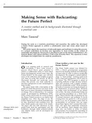
Flight missions are per<strong>for</strong>med in a training area of approximately one<br />
square kilometer in the south of Sweden, called Revinge (Fig.1.1). The area<br />
is used mainly <strong>for</strong> fire fighter training <strong>an</strong>d includes a number of building<br />
structures <strong>an</strong>d road network. An accurate 3D model of the area is available<br />
on board the helicopter in a GIS (Geographic In<strong>for</strong>mation System), which<br />
is used <strong>for</strong> mission pl<strong>an</strong>ning purposes.<br />
Figure 1.1: Orthophoto of the flight-test area in Revinge (south of Sweden).
Chapter 2<br />
Overview<br />
This chapter presents <strong>an</strong> overview of the <strong>UAV</strong> architecture developed during<br />
the WITAS <strong>UAV</strong> Project. The components which have been developed<br />
<strong>an</strong>d are part of this thesis will be considered in this context.<br />
A description of the <strong>UAV</strong> helicopter plat<strong>for</strong>m used <strong>for</strong> the experimental<br />
tests will also be presented. Details of the plat<strong>for</strong>m which are relev<strong>an</strong>t to<br />
this thesis will also be considered in order to gain a better underst<strong>an</strong>ding<br />
of the components developed.<br />
2.1 <strong>UAV</strong> software architecture<br />
The software architecture developed during the WITAS <strong>UAV</strong> Project is a<br />
complex distributed architecture <strong>for</strong> high level autonomous missions. The<br />
architecture enables the <strong>UAV</strong> to per<strong>for</strong>m so-called push button mission.<br />
This is intended to me<strong>an</strong> that a <strong>UAV</strong> is capable of pl<strong>an</strong>ning <strong>an</strong>d executing<br />
a mission from take-off to l<strong>an</strong>ding with limited, or no hum<strong>an</strong> intervention.<br />
An example of such a mission demonstrated in <strong>an</strong> actual flight experiment<br />
is a photogrammetry scenario. In such a scenario a <strong>UAV</strong> helicopter is<br />
given the task of taking pictures of each of the facades of a selected set<br />
of buildings input by a ground operator. The details of this mission are<br />
described in Paper II. To accomplish this kind of mission, <strong>an</strong> architecture<br />
5
6 CHAPTER 2. OVERVIEW<br />
which integrates m<strong>an</strong>y different functionalities is required.<br />
Fig. 2.1 provides a schematic of the software architecture that has been<br />
developed. The modules focused on in this thesis have been emphasized<br />
in the schematic. The boxes emphasized with bold lines <strong>an</strong>d text have<br />
been developed <strong>an</strong>d made operational <strong>an</strong>d will be described in detail in<br />
this thesis.<br />
Figure 2.1: <strong>UAV</strong> software architecture schematic. The modules emphasized<br />
using bold lines are the focus of this thesis.<br />
The software architecture has been implemented using three computers
2.1. <strong>UAV</strong> SOFTWARE ARCHITECTURE 7<br />
which will be described shortly.<br />
• The deliberative/reactive system (DRC) executes a number of high<br />
level functionalities of a deliberative nature such as path pl<strong>an</strong>ner,<br />
execution monitoring, GIS, etc.<br />
• The image processing system (IPC) executes image processing functions<br />
<strong>an</strong>d h<strong>an</strong>dles everything which is related to the video camera<br />
(frame grabbing, camera p<strong>an</strong>/tilt control, etc.).<br />
• The primary flight control system (PFC) executes the control modes<br />
(hovering, path following, take-off, l<strong>an</strong>ding, etc.), the sensor fusion<br />
functions (INS/GPS, INS/camera) <strong>an</strong>d h<strong>an</strong>dles communication with<br />
the helicopter plat<strong>for</strong>m <strong>an</strong>d with the other sensors (GPS, pressure<br />
sensor, etc.).<br />
The PFC executes predomin<strong>an</strong>tly hard real-time tasks such as the flight<br />
control modes or the sensor fusion algorithms. This part of the system uses<br />
a Real-Time Application Interface (RTAI) [14] which provides industrialgrade<br />
real-time operating system functionality. RTAI is a hard real-time<br />
extension to a st<strong>an</strong>dard Linux kernel (Debi<strong>an</strong>) <strong>an</strong>d has been developed at<br />
the Department of Aerospace Engineering of Politecnico di Mil<strong>an</strong>o. The<br />
DRC has reduced timing requirements. This part of the system uses the<br />
Common Object Request Broker Architecture (CORBA) as its distribution<br />
backbone. Currently <strong>an</strong> open source implementation of CORBA 2.6<br />
called TAO/ACE [11] is in use. More details about the complete software<br />
architecture c<strong>an</strong> be found in Paper III <strong>an</strong>d in [3, 15].<br />
As c<strong>an</strong> be observed from the boxes emphasized in Fig. 2.1, this thesis<br />
deals with a number of functionalities which are contained in the PFC<br />
system. A brief introduction as to what these functionalities actually do<br />
will now be described.<br />
The simulator mentioned in the introduction implements the helicopter<br />
dynamics. Moreover it emulates the helicopter sensor outputs so that during<br />
the simulation the complete software architecture c<strong>an</strong> be tested in a<br />
closed loop. The simulator c<strong>an</strong> also run on the on board hardware so that<br />
during the simulation it is possible to see the helicopter actuators moving<br />
as they would in actual flight. Such simulation using hardware-in-the-loop
8 CHAPTER 2. OVERVIEW<br />
provides a powerful way to quickly test the correct functioning of all the<br />
components on the field, including the interface to the helicopter.<br />
The path following control mode (PFCM) enables the helicopter to<br />
follow a 3D path. It receives a geometric description of a path via a number<br />
of parameters from the path pl<strong>an</strong>ner. From these parameters it generates<br />
a continuous description of the path, then it adds velocity <strong>an</strong>d acceleration<br />
constraints in order to calculate the inputs to be sent to the helicopter. An<br />
algorithm which generates the proper control inputs at each control cycle<br />
has been developed. The PFCM also generates a number of events <strong>an</strong>d<br />
other outputs which are necessary <strong>for</strong> monitoring purposes in flight.<br />
The two sensor fusion algorithms implemented are based on a Kalm<strong>an</strong><br />
filter <strong>an</strong>d produce estimates of the helicopter state in terms of position, velocity<br />
<strong>an</strong>d attitude. They are used to fuse the inertial sensors with the GPS,<br />
<strong>an</strong>d the inertial sensors with the video camera during autonomous l<strong>an</strong>ding.<br />
Since they are based on the same dynamic model, only the results of the<br />
integration between inertial sensors <strong>an</strong>d video camera will be presented. It<br />
will be shown how the integration of the video camera with inertial sensors<br />
c<strong>an</strong> effectively improve the robustness of the helicopter state estimate<br />
compared to a solution obtained from image processing alone.<br />
2.2 The <strong>UAV</strong> helicopter plat<strong>for</strong>m<br />
The Yamaha RMAX helicopter used <strong>for</strong> the experimentation (Fig. 2.2) has<br />
a total length of 3.6 m (including main rotor). It is powered by a 21 hp<br />
two-stroke engine <strong>an</strong>d has a maximum takeoff weight of 95 kg.<br />
The RMAX rotor head is equipped with a Bell-Hiller stabilizer bar<br />
(see Fig.2.3). The effect of the Bell-Hiller mech<strong>an</strong>ism is to reduce the<br />
response of the helicopter to wind gusts. Moreover, the stabilizer bar is<br />
used to generate a control augmentation to the main rotor cyclic input.<br />
The Bell-Hiller mech<strong>an</strong>ism is very common in small-scale helicopters but<br />
quite uncommon in full-scale helicopters. The reason <strong>for</strong> this is that a<br />
small-scale helicopter experiences less rotor-induced damping compared to<br />
full-scale helicopters. Consequently, it is more difficult to control <strong>for</strong> a<br />
hum<strong>an</strong> pilot. It should be pointed out though that <strong>an</strong> electronic control<br />
system c<strong>an</strong> stabilize a small-scale helicopter without a stabilizer bar quite
2.2. THE <strong>UAV</strong> HELICOPTER PLATFORM 9<br />
Figure 2.2: The RMAX helicopter.<br />
efficiently. For this reason the trend <strong>for</strong> small-scale autonomous helicopters<br />
is to remove the stabilizer bar <strong>an</strong>d let the digital control system stabilize the<br />
helicopter. The adv<strong>an</strong>tage in this case is reduced mech<strong>an</strong>ical complexity in<br />
the system.<br />
Figure 2.3: The RMAX rotor head with Bell-Hiller mech<strong>an</strong>ism.
10 CHAPTER 2. OVERVIEW<br />
The RMAX helicopter has a built-in attitude sensor called YAS (Yamaha<br />
Attitude Sensor) composed of three accelerometers <strong>an</strong>d three rate gyros.<br />
The output of the YAS are acceleration <strong>an</strong>d <strong>an</strong>gular rate on the three helicopter<br />
body axes (see section 3.3 <strong>for</strong> a definition of body axis). The YAS<br />
also computes the helicopter attitude <strong>an</strong>gles. Acceleration <strong>an</strong>d <strong>an</strong>gular<br />
rate from the YAS will be used as inertial measurement data <strong>for</strong> the sensor<br />
fusion process which will be described in chapter 5.<br />
The RMAX also has a built-in digital attitude control system called<br />
YACS (Yamaha Attitude Control System). The YACS stabilizes the helicopter<br />
attitude dynamics <strong>an</strong>d the vertical ch<strong>an</strong>nel dynamics. The YACS is<br />
used in all the helicopter control modes as <strong>an</strong> attitude stabilization system.<br />
The hardware plat<strong>for</strong>m developed during the WITAS <strong>UAV</strong> Project is<br />
integrated with the Yamaha plat<strong>for</strong>m as shown in Fig. 2.4. It is based on<br />
three PC104 embedded computers.<br />
DRC<br />
- 1.4 GHz P-M<br />
- 1GB RAM<br />
- 512 MB flash<br />
IPC<br />
- 700 MHz PIII<br />
- 256MB RAM<br />
- 512 MB flash<br />
sensor<br />
suite<br />
RS232C<br />
Ethernet<br />
Other media<br />
ethernet<br />
switch<br />
PFC<br />
- 700 MHz PIII<br />
- 256MB RAM<br />
- 512 MB flash<br />
sensor<br />
suite<br />
Yamaha RMAX<br />
(YAS, YACS)<br />
Figure 2.4: On-board hardware schematic.
2.2. THE <strong>UAV</strong> HELICOPTER PLATFORM 11<br />
The PFC is implemented on a 700Mhz Pentium III <strong>an</strong>d includes a wireless<br />
Ethernet bridge, a GPS receiver <strong>an</strong>d a barometric altitude sensor. An<br />
earlier version of the system included a compass as a heading sensor source.<br />
The compass has been removed from the latest version since the Kalm<strong>an</strong><br />
filter which fuses the inertial sensors <strong>an</strong>d GPS provides sufficiently stable<br />
heading in<strong>for</strong>mation. The PFC communicates with the helicopter through<br />
a serial line RS232C, where the inertial sensor data from the YAS is passed<br />
to the PFC. The PFC c<strong>an</strong> also send control inputs to the YACS <strong>for</strong> helicopter<br />
control. The IPC runs on a second PC104 embedded computer<br />
(PIII 700MHz), <strong>an</strong>d includes a color CCD camera mounted on a p<strong>an</strong>/tilt<br />
unit, a video tr<strong>an</strong>smitter <strong>an</strong>d a video recorder (miniDV). The DRC system<br />
runs on the third PC104 embedded computer (Pentium-M 1.4GHz) <strong>an</strong>d<br />
executes all high-end autonomous functionality. Network communication<br />
between computers is physically realized with serial line RS232C <strong>an</strong>d Ethernet.<br />
Ethernet is mainly used <strong>for</strong> CORBA applications, remote login <strong>an</strong>d<br />
file tr<strong>an</strong>sfer, while serial lines are used <strong>for</strong> hard real-time networking.
12 CHAPTER 2. OVERVIEW
Chapter 3<br />
Simulation<br />
3.1 Introduction<br />
This chapter describes the simulation tool which has been used to develop<br />
<strong>an</strong>d test the control system <strong>for</strong> the RMAX helicopter. It is used to test the<br />
helicopter missions both in the lab <strong>an</strong>d on the field. The RMAX helicopter<br />
simulator is implemented in the C l<strong>an</strong>guage <strong>an</strong>d allows testing of all the<br />
control modes developed. M<strong>an</strong>y flight-test hours have been avoided due<br />
to the possibility of running, in simulation, the exact code of the control<br />
system which is executed on the on-board computer during the actual flighttest.<br />
In order to develop <strong>an</strong>d test the helicopter control system a mathematical<br />
model which represents the dynamic behavior of the helicopter<br />
is required. The simulator described in this section is specialized <strong>for</strong> the<br />
Yamaha RMAX helicopter in the sense that the model includes the dynamics<br />
of the bare plat<strong>for</strong>m in addition to the Yamaha Attitude Control<br />
System (YACS).<br />
The YACS system stabilizes the pitch <strong>an</strong>d roll <strong>an</strong>gles of the helicopter,<br />
the yaw rate <strong>an</strong>d the vertical velocity. The reason why the YACS has been<br />
used was to speed up the control development process <strong>an</strong>d to shift the<br />
focus toward development of functionalities such as the PFCM presented<br />
13
14 CHAPTER 3. SIMULATION<br />
in chapter 4. All of the currently developed flight modes use the YACS as <strong>an</strong><br />
inner control loop which stabilizes the high frequency helicopter dynamics.<br />
Experimental tests have shown that the YACS decouples the helicopter<br />
dynamics so that the pitch, roll, yaw <strong>an</strong>d vertical ch<strong>an</strong>nels c<strong>an</strong> be treated<br />
separately in the control system design. In other words the ch<strong>an</strong>nels do<br />
not influence each other.<br />
3.2 Hardware-in-the-loop simulation<br />
Two versions of the simulator have been developed. A non real-time version<br />
exists which is used to develop the control modes, where the purpose of<br />
the simulation in this case is the tuning <strong>an</strong>d testing of the internal logic<br />
of the control modes. A real-time version also exists which is used to<br />
test the complete <strong>UAV</strong> architecture, where simulations are per<strong>for</strong>med with<br />
the helicopter hardware-in-the-loop. The latter is used to test a complete<br />
helicopter mission <strong>an</strong>d c<strong>an</strong> be used on the flight-test field as a last minute<br />
verification <strong>for</strong> the correct functioning of hardware <strong>an</strong>d software. Both<br />
simulators use the same dynamic model which will be presented in this<br />
chapter.<br />
The helicopter dynamics function is located in the PFC system <strong>an</strong>d it<br />
is called every 20ms when the system is in simulation mode. Fig. 3.1 shows<br />
the hardware/software components involved in the real flight-test <strong>an</strong>d in<br />
the simulation test. The components <strong>an</strong>d connections represented with a<br />
dashed line are not active during the respective test modalities.<br />
The diagram shows which components c<strong>an</strong> be tested in simulation. Observe<br />
that in simulation the helicopter servos are connected <strong>an</strong>d c<strong>an</strong> move,<br />
but there is no feedback from the servo position to the simulator. The fact<br />
that their movement c<strong>an</strong> be visually checked is used as a final check that<br />
the system is operating appropriately.<br />
The YACS control system is also part of the loop, but since it is built<br />
into the helicopter, it c<strong>an</strong>not be fed with simulated sensor outputs, so it<br />
still takes the input from the YAS sensor which, obviously, does not deliver<br />
<strong>an</strong>y measurement from the helicopter. This is not problematic because the<br />
simulator does not have the purpose of testing the correct functioning of<br />
the YACS.
3.2. HARDWARE-IN-THE-LOOP SIMULATION 15<br />
Figure 3.1: Figure a) depicts the hardware/software architecture in flighttest<br />
configuration. Figure b) depicts the architecture during the hardwarein-the-loop<br />
simulation.
16 CHAPTER 3. SIMULATION<br />
Currently, the video camera is not used in the simulation loop but<br />
the system c<strong>an</strong> still control the camera p<strong>an</strong>/tilt. A virtual environment<br />
(Fig. 3.2), reproducing the flight-test area described in the introduction<br />
(Fig.1.1), is used <strong>for</strong> visualization purposes. Theoretically the image processing<br />
functions could be fed with synthetic images in order to feedback<br />
from the virtual environment, this is a topic <strong>for</strong> future work.<br />
Figure 3.2: Virtual environment used <strong>for</strong> flight mission simulation.
3.3. REFERENCE FRAMES 17<br />
3.3 Reference frames<br />
This section provides <strong>an</strong> overview of the different reference frames used in<br />
this thesis.<br />
The Earth frame (Fig. 3.3) has its origin at the center of mass of the<br />
Earth <strong>an</strong>d axes which are fixed with respect to the Earth. Its Xe axis<br />
points toward the me<strong>an</strong> meridi<strong>an</strong> of Greenwich, the Ze axis is parallel to<br />
the me<strong>an</strong> spin axis of the Earth, <strong>an</strong>d the Ye axis completes a right-h<strong>an</strong>ded<br />
orthogonal frame.<br />
The navigation frame (Fig. 3.3) is a local geodetic frame which has<br />
its origin coinciding with that of the sensor frame <strong>an</strong>d axes with the Xn<br />
axis pointing toward the geodetic north, the Zn axis orthogonal to the reference<br />
ellipsoid pointing down, <strong>an</strong>d the Yn axis completing a right-h<strong>an</strong>ded<br />
orthogonal frame.<br />
Figure 3.3: Earth <strong>an</strong>d navigation frames.<br />
The body frame (Fig. 3.4) is <strong>an</strong> orthogonal axis set which has its origin<br />
coinciding with the center of gravity of the helicopter, the Xb axis pointing<br />
<strong>for</strong>ward to the nose, the y-axis orthogonal to the Yb axis <strong>an</strong>d pointing to<br />
the right side of the helicopter body, <strong>an</strong>d the Zb axis pointing down so that
18 CHAPTER 3. SIMULATION<br />
it’s a right-h<strong>an</strong>ded orthogonal frame. Since the RMAX inertial sensors are<br />
quite close to the helicopter’s center of gravity it is possible to consider the<br />
navigation frame <strong>an</strong>d the body frame as having the same origin point.<br />
Figure 3.4: Body frame.<br />
In order to tr<strong>an</strong>s<strong>for</strong>m a vector from the body frame to the navigation<br />
frame a rotation matrix has to be applied:<br />
C n b =<br />
⎡<br />
⎤<br />
cosθcosψ −cosφsinψ+sinφsinθcosψ sinφsinψ+cosφsinθcosψ<br />
⎣ cosθsinψ cosφcosψ+sinφsinθsinψ −sinφcosψ+cosφsinθsinψ⎦(3.1)<br />
−sinθ sinφcosθ cosφcosθ<br />
where φ, θ <strong>an</strong>d ψ are the Euler <strong>an</strong>gles roll, pitch <strong>an</strong>d heading. Since<br />
the rotation matrix is orthogonal, the tr<strong>an</strong>s<strong>for</strong>mation from the navigation<br />
frame to the body frame is given by:<br />
C b n=(C n b ) T<br />
(3.2)<br />
The tr<strong>an</strong>s<strong>for</strong>mation matrix 3.1 <strong>an</strong>d 3.2 will be used later in the thesis.
3.4. THE AUGMENTED RMAX DYNAMIC MODEL 19<br />
3.4 The augmented RMAX dynamic model<br />
The RMAX helicopter model presented in this thesis includes the bare helicopter<br />
dynamics <strong>an</strong>d the YACS control system dynamics. The code of the<br />
YACS is strictly Yamaha proprietary so the approach used to build the relative<br />
mathematical model has been that of black-box model identification.<br />
With the use of this technique, it is possible to estimate the mathematical<br />
model of <strong>an</strong> unknown system (the only hypothesis about the system is that<br />
it has a linear behavior) just by observing its behavior. This is achieved in<br />
practice by sending <strong>an</strong> input signal to the system <strong>an</strong>d measuring its output.<br />
Once the input <strong>an</strong>d output signals are known there are several methods to<br />
identify the mathematical structure of the system.<br />
The YACS model identification is not part of this thesis <strong>an</strong>d details<br />
c<strong>an</strong> be found in [4]. In the following section the tr<strong>an</strong>sfer functions of the<br />
augmented attitude dynamics will be given. These tr<strong>an</strong>sfer functions will<br />
be used to build the augmented RMAX helicopter dynamic model used in<br />
the simulator.<br />
3.4.1 Augmented helicopter attitude dynamics<br />
As previously stated the YACS <strong>an</strong>d helicopter attitude dynamics have been<br />
identified through black-box model identification.<br />
The equations 3.3 represent the four input/output tr<strong>an</strong>sfer functions in<br />
the Laplace domain:<br />
∆Φ =<br />
∆Θ =<br />
∆R =<br />
∆AZ =<br />
2.3(s 2 + 3.87s + 53.3)<br />
(s 2 + 6.29s + 16.2)(s 2 + 8.97s + 168) ∆AIL<br />
0.5(s 2 + 9.76s + 75.5)<br />
(s 2 + 3s + 5.55)(s 2 + 2.06s + 123.5)<br />
9.7(s + 12.25)<br />
(s + 4.17)(s2 + 3.5s + 213.4) ∆RUD<br />
0.0828s(s + 3.37)<br />
(s + 0.95)(s2 ∆T HR<br />
+ 13.1s + 214.1)<br />
∆ELE (3.3)<br />
where ∆Φ <strong>an</strong>d ∆Θ are the roll <strong>an</strong>d pitch <strong>an</strong>gle increments (deg), ∆R
20 CHAPTER 3. SIMULATION<br />
the body yaw <strong>an</strong>gular rate increment (deg/sec) <strong>an</strong>d ∆AZ the acceleration<br />
increment (g) along the Zb body axis. ∆AIL, ∆ELE, ∆RUD <strong>an</strong>d ∆T HR<br />
are the control input increments taken relative to a trimmed flight condition.<br />
The control inputs are in YACS unit <strong>an</strong>d r<strong>an</strong>ge from -500 <strong>an</strong>d +500.<br />
These tr<strong>an</strong>sfer functions describe not only the dynamic behavior of the<br />
YACS but also the dynamics of the helicopter (rotor <strong>an</strong>d body) <strong>an</strong>d the<br />
dynamics of the actuators.<br />
Since the chain composed by the YACS, actuators <strong>an</strong>d helicopter is<br />
quite complex it is import<strong>an</strong>t to remember that the estimated model has<br />
only picked up a simple reflection of the system behavior. The identification<br />
was done near the hovering condition so it is improper to use the model<br />
<strong>for</strong> different flight conditions. In spite of this, simulations up to ∼10 m/s<br />
have shown good agreement with the experimental flight-test results.<br />
3.4.2 <strong>Helicopter</strong> equations of motion<br />
The aircraft equations of motion c<strong>an</strong> be expressed in the body reference<br />
frame with three sets of first order differential equations [7]. The first set<br />
represents the tr<strong>an</strong>slational dynamics along the three body axes:<br />
X = m( ˙u + qw − rv) + mgsinθ<br />
Y = m( ˙v + ru − pw) − mgcosθsinφ (3.4)<br />
Z = m( ˙w + pv − qu) − mgcosθcosφ<br />
where X, Y , Z represent the result<strong>an</strong>ts of all the aerodynamic <strong>for</strong>ces; u,<br />
v, w the body velocity components; p, q, r the body <strong>an</strong>gular rates; m <strong>an</strong>d<br />
g the mass <strong>an</strong>d the gravity acceleration; φ <strong>an</strong>d θ the pitch <strong>an</strong>d roll <strong>an</strong>gles.<br />
The second set of equations represents the aircraft rotational dynamics:<br />
L = Ix ˙p − (Iy − Iz)qr<br />
M = Iy ˙q − (Iz − Ix)rp (3.5)<br />
N = Iz ˙r − (Ix − Iy)pq<br />
where L, M, N represent the moments generated by the aerodynamic<br />
<strong>for</strong>ces acting on the helicopter; Ix, Iy, Iz the inertia moments of the helicopter.
3.4. THE AUGMENTED RMAX DYNAMIC MODEL 21<br />
The third set of equations represents the relation between the body<br />
<strong>an</strong>gular rates <strong>an</strong>d the Euler <strong>an</strong>gles:<br />
˙φ = p + qsinφt<strong>an</strong>θ + rcosφt<strong>an</strong>θ<br />
˙θ = qcosφ − rsinφ (3.6)<br />
˙ψ = qsinφsecθ + rcosφsecθ<br />
These three sets of nonlinear equations are valid <strong>for</strong> a generic aircraft.<br />
The tr<strong>an</strong>sfer functions in 3.3 c<strong>an</strong> be used now in the motion equations.<br />
From the Laplace domain of the tr<strong>an</strong>sfer functions, it is possible to pass<br />
to the time domain. This me<strong>an</strong>s that from the first three equations in 3.3<br />
we derive φ(t), θ(t) <strong>an</strong>d r(t) which c<strong>an</strong> be used in 3.6 in order to find the<br />
other parameters p(t), q(t), ψ(t).<br />
The equations in 3.5 will not be used in the model because the dynamics<br />
represented by these equations is contained in the first three tr<strong>an</strong>sfer<br />
functions in 3.3. The motion equations in 3.4 c<strong>an</strong> be rewritten as follows:<br />
˙u = Fx − qw + rv − gsinθ<br />
˙v = Fy − ru + pw + gcosθsinφ (3.7)<br />
˙w = Fz − pv + qu + gcosθcosφ<br />
where Fx, Fy, Fz are the <strong>for</strong>ces per unit of mass. In this set of equations<br />
some of the nonlinear terms are small <strong>an</strong>d c<strong>an</strong> be neglected <strong>for</strong> our flight<br />
envelope, although <strong>for</strong> simulation purposes, it does not hurt to leave them<br />
there. Later when the model will be used <strong>for</strong> control purposes the necessary<br />
simplifications will be made.<br />
The tail rotor <strong>for</strong>ce is included in Fy <strong>an</strong>d it is bal<strong>an</strong>ced by a certain<br />
amount of roll <strong>an</strong>gle. In fact every helicopter with a tail rotor must fly<br />
with a few degrees of roll <strong>an</strong>gle in order to compensate <strong>for</strong> the tail rotor<br />
<strong>for</strong>ce which is directed sideway. For the RMAX helicopter the roll <strong>an</strong>gle<br />
is 4.5 deg in hovering condition with no wind. The yaw dynamics in our<br />
case is represented by the third tr<strong>an</strong>sfer function in 3.3. For this reason<br />
we do not have to model the <strong>for</strong>ce explicitly. By doing that we find in our<br />
model a zero degree roll <strong>an</strong>gle in hovering condition which does not affect
22 CHAPTER 3. SIMULATION<br />
subst<strong>an</strong>tially the dynamics of our simulator. Of course a small coupling<br />
effect between the lateral helicopter motion <strong>an</strong>d yaw ch<strong>an</strong>nel is neglected<br />
during a fast yaw m<strong>an</strong>euver due to the consistent increase of the tail rotor<br />
<strong>for</strong>ce.<br />
The equations in 3.7 are th<strong>an</strong> rewritten in find <strong>for</strong>m as follows:<br />
˙u = Xuu − qw + rv − gsinθ<br />
˙v = Yvv − ru + pw + gcosθsinφ (3.8)<br />
˙w = Zww + T − pv + qu + gcosθcosφ<br />
where Xu, Yv <strong>an</strong>d Zw are the aerodynamic derivatives (accounting <strong>for</strong><br />
the aerodynamic drag). The value used <strong>for</strong> the aerodynamic derivatives are<br />
Xu = −0.025, Yv = −0.1 <strong>an</strong>d Zw = −0.6. These values have been chosen<br />
using <strong>an</strong> empirical best fit criteria using flight-test data.<br />
The main rotor thrust T is given by:<br />
T = −g − ∆aZ<br />
(3.9)<br />
where ∆aZ is given by the fourth tr<strong>an</strong>sfer function in 3.3.<br />
Comparing the equations in 3.8 with other works in the literature as <strong>for</strong><br />
example in [16] it c<strong>an</strong> be noticed that the rotor flapping terms are missing<br />
(the rotor flapping represents the possibility of the helicopter rotor disk to<br />
tilt relatively to the helicopter fuselage). On the other h<strong>an</strong>d the flapping<br />
dynamics is contained in the tr<strong>an</strong>sfer functions in 3.3. It was not possible<br />
to model the rotor flapping explicitly in the equations 3.8 because it is not<br />
observable from the black-box model identification approach used. The<br />
fact that the flapping terms are not included in equations 3.8 does not have<br />
strong consequences on the low frequency dynamics. On the other h<strong>an</strong>d the<br />
high frequency helicopter dynamics is not captured correctly. There<strong>for</strong>e the<br />
helicopter model derived here c<strong>an</strong>not be used <strong>for</strong> high b<strong>an</strong>dwidth control<br />
system design. The model <strong>an</strong>yway is good enough <strong>for</strong> position <strong>an</strong>d velocity<br />
control loop design. In [20] the mathematical <strong>for</strong>mulation <strong>for</strong> rotor flapping<br />
c<strong>an</strong> be found.
3.5. SIMULATION RESULTS 23<br />
3.5 Simulation results<br />
The validation of the RMAX helicopter model c<strong>an</strong> be found in [4]. In this<br />
section, the validation of the simulation procedure with the control system<br />
in the loop will be described. The results of two simulation tests of the<br />
PFCM, which will also be described later in the thesis, will be provided.<br />
The PFCM is a control function that enables the helicopter to follow 3D<br />
path segments. The path segments will be given to the PFCM which is in<br />
a closed loop with the simulator. The simulation results will be compared<br />
to the same PFCM implemented on the helicopter plat<strong>for</strong>m. This is not a<br />
validation of the simulator since the control function is in the loop. What<br />
is interesting is the <strong>an</strong>alysis of the differences of the closed loop behavior<br />
between the flight-test <strong>an</strong>d the simulation. The helicopter is comm<strong>an</strong>ded<br />
to fly a segment path starting from a hovering condition until reaching a<br />
target speed. The path also presents a curvature ch<strong>an</strong>ge. The same control<br />
function has been used <strong>for</strong> the two tests. In Fig. 3.5 <strong>an</strong>d Fig. 3.6 the<br />
simulation (dashed line) <strong>an</strong>d flight-test (continuous line) are overlapped on<br />
the same graph. The upper-left plot of Fig. 3.5 represents the helicopter<br />
path seen from above. The difference in position between the simulation<br />
<strong>an</strong>d flight-test is very small, below one meter <strong>an</strong>d c<strong>an</strong>not be seen in detail<br />
from the plot. In the same diagram the velocity components <strong>an</strong>d the total<br />
velocity are plotted. This shows that the simulated velocity <strong>an</strong>d the real<br />
velocity are quite close. In this test the helicopter was accelerated to 5 m/s<br />
<strong>for</strong>ward speed. In Fig. 3.6 the results <strong>for</strong> the pitch <strong>an</strong>d roll inputs <strong>an</strong>d the<br />
attitude <strong>an</strong>gles are presented. The pitch <strong>an</strong>d roll inputs present a steady<br />
state error compared to the simulation while the pitch <strong>an</strong>d roll <strong>an</strong>gles are<br />
in good agreement.<br />
In Fig. 3.7 <strong>an</strong>d Fig. 3.8 the same path segment is tested but the helicopter<br />
accelerates until 10 m/s is reached. The simulated position <strong>an</strong>d<br />
velocity are still in good agreement with the flight-test experiment while<br />
the pitch <strong>an</strong>d roll <strong>an</strong>gles are worse. This is due to the fact that the aerodynamics<br />
of the rotor is not modeled. Taking into account such effects is<br />
necessary <strong>for</strong> flight conditions far from hovering. It is interesting to notice<br />
that the simulation c<strong>an</strong> predict quite accurately the saturation of the roll<br />
input (Fig. 3.8) at around 845 sec. This could be a sign that the helicopter<br />
is flying too fast <strong>for</strong> the current path curvature, <strong>an</strong>d <strong>an</strong> adjustment in the
24 CHAPTER 3. SIMULATION<br />
PFCM in the generation of the velocity reference might be required. This<br />
kind of problem c<strong>an</strong> be <strong>an</strong>alyzed very efficiently with the simulator tool<br />
developed.<br />
Figure 3.5: Results 1st flight. Comparison between flight-test position<br />
<strong>an</strong>d velocity data (solid) with simulation data (dash-dot). The helicopter<br />
accelerates to 5 m/s target velocity.
3.5. SIMULATION RESULTS 25<br />
Figure 3.6: Results 1st flight. Comparison between flight-test helicopter<br />
inputs <strong>an</strong>d attitude data (solid) with simulation data (dash-dot). The<br />
helicopter accelerates to 5 m/s target velocity.
26 CHAPTER 3. SIMULATION<br />
Figure 3.7: Results 2nd flight. Comparison between flight-test position<br />
<strong>an</strong>d velocity data (solid) with simulation data (dash-dot). The helicopter<br />
accelerates to 10 m/s target velocity.
3.5. SIMULATION RESULTS 27<br />
Figure 3.8: Results 2nd flight. Comparison between flight-test helicopter<br />
inputs <strong>an</strong>d attitude data (solid) with simulation data (dash-dot). The<br />
helicopter accelerates to 10 m/s target velocity.
28 CHAPTER 3. SIMULATION<br />
3.6 Conclusion<br />
In this chapter the simulation tool used to test <strong>an</strong>d develop the <strong>UAV</strong> software<br />
architecture including the control system has been described. The<br />
simulator has been a useful tool <strong>for</strong> the development of the control modes.<br />
The hardware-in-the-loop version of the simulator is a useful tool to test<br />
a complete mission on the field. In addition, the fact that the helicopter<br />
servos are in the simulation loop provides a rapid verification that the right<br />
signals arrive from the control system. This verification is used <strong>for</strong> a final<br />
decision on the field in order to proceed or not with a flight-test.
Chapter 4<br />
Path Following Control<br />
Mode<br />
4.1 Introduction<br />
The PFCM described in this chapter <strong>an</strong>d presented in Paper I, has been<br />
designed to navigate <strong>an</strong> autonomous helicopter in <strong>an</strong> area cluttered with<br />
obstacles, such as <strong>an</strong> urb<strong>an</strong> environment. In this thesis, the path pl<strong>an</strong>ning<br />
problem is not addressed although it is in [18]. It is assumed that a<br />
path pl<strong>an</strong>ning functionality generates a collision-free path. Then the task<br />
which will be solved here is to find a suitable guid<strong>an</strong>ce <strong>an</strong>d control law<br />
which enables the helicopter to follow the path robustly. The path pl<strong>an</strong>ner<br />
calculates the geometry of the path that the helicopter has to follow. A<br />
geometric path segment, represented by a set of parameters, is then input<br />
to the PFCM.<br />
Be<strong>for</strong>e starting with the description of the PFCM, some basic terminology<br />
will be provided.<br />
The guid<strong>an</strong>ce is the process of directing the movements of <strong>an</strong> aeronautical<br />
vehicle with particular reference to the selection of a flight path.<br />
The term of guid<strong>an</strong>ce or trajectory generation in this thesis addresses the<br />
problem of generating the desired reference position <strong>an</strong>d velocity <strong>for</strong> the<br />
29
30 CHAPTER 4. PATH FOLLOWING CONTROL MODE<br />
helicopter at each control cycle.<br />
The outer control is a feedback loop which takes as inputs the reference<br />
position <strong>an</strong>d velocity generated by the trajectory generator <strong>an</strong>d calculates<br />
the output <strong>for</strong> <strong>an</strong> inner control loop.<br />
The inner control is a feedback loop which stabilizes the helicopter<br />
attitude <strong>an</strong>d the vertical dynamics. As mentioned previously, the inner<br />
control loop used here has been developed by Yamaha Motor Comp<strong>an</strong>y<br />
<strong>an</strong>d is part of the YACS.<br />
Several methods have been proposed to solve the problem of generation<br />
<strong>an</strong>d execution of a state-space trajectory <strong>for</strong> <strong>an</strong> autonomous helicopter [6,<br />
9]. In general this is a hard problem, especially when the trajectory is time<br />
dependent. The solution adopted here is to separate the problem into two<br />
parts: first to find a collision-free path in the space domain [18] <strong>an</strong>d th<strong>an</strong><br />
to add a velocity profile later. In this way the position of the helicopter is<br />
not time dependent which me<strong>an</strong>s that it is not required <strong>for</strong> the helicopter<br />
to be in a certain point at a specific time. A convenient approach <strong>for</strong> such a<br />
problem is the path following method. By using the path following method<br />
the helicopter is <strong>for</strong>ced to fly close to the geometric path with a specified<br />
<strong>for</strong>ward speed. In other words, the path is always prioritized <strong>an</strong>d this is<br />
a requirement <strong>for</strong> robots that <strong>for</strong> example have to follow roads <strong>an</strong>d avoid<br />
collisions with buildings. The method developed <strong>for</strong> PFCM is weakly model<br />
dependent <strong>an</strong>d computationally efficient.<br />
The path following method has also been <strong>an</strong>alyzed in [24, 22]. The<br />
guid<strong>an</strong>ce law derived there presents singularity when the cross-track error<br />
is equal to the curvature radius of the path so that it has a restriction on the<br />
allowable cross-track error. The singularity arises because the guid<strong>an</strong>ce law<br />
is obtained by using the Serret-Frenet <strong>for</strong>mulas <strong>for</strong> curves in the pl<strong>an</strong>e [24].<br />
The approach used in this thesis does not use the Serret-Frenet <strong>for</strong>mulas<br />
but a different guid<strong>an</strong>ce algorithm similar to the one described in [5] which<br />
is also known as virtual leader. In this case the motion of the control point<br />
on the desired path is governed by a differential equation containing error<br />
feedback which gives great robustness to the guid<strong>an</strong>ce method. The control<br />
point (Fig. 4.1) is basically a point lying on the path where the helicopter<br />
ideally should be.<br />
The guid<strong>an</strong>ce algorithm developed uses in<strong>for</strong>mation from the model<br />
in 3.8 described in section 3.4.2 in order to improve the path tracking
4.2. TRAJECTORY GENERATOR 31<br />
Figure 4.1: Control point on the reference path.<br />
error while maintaining a reasonable flight speed. The experimental results<br />
presented show the validity of the control approach.<br />
Fig. 4.2 represents the different components of the control system, from<br />
the path pl<strong>an</strong>ner to the inner loop that directly sends the control inputs to<br />
the helicopter actuators. The PFCM described in this thesis includes the<br />
trajectory generator <strong>an</strong>d the outer control loop.<br />
4.2 Trajectory generator<br />
In this section, a description of the guid<strong>an</strong>ce algorithm developed <strong>for</strong> the<br />
PFCM is provided. The trajectory generator function takes as input a set of<br />
parameters describing the geometric path calculated by the path pl<strong>an</strong>ner<br />
<strong>an</strong>d calculates the reference position, velocity <strong>an</strong>d heading <strong>for</strong> the inner<br />
control loop. First the <strong>an</strong>alytic expression of the 3D path is calculated,<br />
then a feedback algorithm calculates the control point on the path. Finally<br />
the reference input <strong>for</strong> the outer loop is calculated using the kinematic<br />
helicopter model described in chapter 3.
32 CHAPTER 4. PATH FOLLOWING CONTROL MODE<br />
Figure 4.2: The PFCM includes two modules: trajectory generator <strong>an</strong>d<br />
outer loop.<br />
4.2.1 Calculation of the path geometry<br />
The path pl<strong>an</strong>ner generates 3D geometric paths described by a sequence of<br />
segments. Each segment is passed from the high-level part of the software<br />
architecture, where the path pl<strong>an</strong>ner is located, to the low-level part where<br />
the control modes including the PFCM are implemented.<br />
The path segment is generated in the navigation frame with the origin<br />
fixed at the initial point of the path. We will use the superscript n to<br />
indicate a vector in the navigation frame. Each segment is described by<br />
a parameterized 3D cubic curve represented by the following equation in<br />
vectorial <strong>for</strong>m:<br />
P n (s) = As 3 + Bs 2 + Cs + D (4.1)<br />
where A, B, C <strong>an</strong>d D are 3D vectors calculated from the boundary<br />
conditions of the segment with s as the segment parameter.
4.2. TRAJECTORY GENERATOR 33<br />
Fig. 4.3 depicts a path segment with the relative boundary conditions.<br />
The segment is defined by the starting point coordinates P (0), the end<br />
point coordinates P (1) <strong>an</strong>d two vectors which represent the direction of<br />
the segment t<strong>an</strong>gent at the starting point P ′ (0) <strong>an</strong>d at the end point P ′ (1)<br />
so that the 3D path segment is defined by 12 parameters. The path pl<strong>an</strong>ner<br />
[18] calculates the 12 parameters ensuring the continuity of the path<br />
<strong>an</strong>d of the first order derivative at the segment joints.<br />
Figure 4.3: Boundary conditions <strong>for</strong> a path segment.<br />
Actually by imposing only these boundary conditions (continuity of the<br />
path <strong>an</strong>d continuity of the first order derivative at the segment joints) the<br />
segment has two degrees of freedom undefined which are represented by<br />
the magnitude of the t<strong>an</strong>gent vectors P ′ (0) <strong>an</strong>d P ′ (1).<br />
The magnitude of the t<strong>an</strong>gent vector affects the curvature of the path.<br />
If the continuity of the second order derivative at the joints (e.g. the<br />
curvature) is imposed then all the 12 parameters would be found <strong>an</strong>d in<br />
this case the path would be a cubic spline [21]. The two degrees of freedom<br />
are chosen by the path pl<strong>an</strong>ner in order to satisfy other conditions which<br />
will not be mentioned here. For more details the reader is referred to [18].
34 CHAPTER 4. PATH FOLLOWING CONTROL MODE<br />
The path generated in this way c<strong>an</strong> have discontinuity of the second order<br />
derivative at the segment joints. This c<strong>an</strong> lead to a small path tracking<br />
error especially at high speed.<br />
The 12 parameters are passed as input arguments to the PFCM which<br />
then generates the reference geometric segment used <strong>for</strong> control purposes.<br />
The generation of the path segment in the PFCM is done using the matrix<br />
<strong>for</strong>mulation in 4.2 with the boundary condition vector explicitly written on<br />
the right h<strong>an</strong>d side. The parameter s r<strong>an</strong>ges from s = 0 which corresponds<br />
to the starting point P (0) to s = 1 which corresponds to the end point<br />
P (1) of the same segment. When the helicopter enters the next segment<br />
the parameter is reset to zero.<br />
P n (s) = � s3 s2 s 1 �<br />
⎡<br />
⎤ ⎡<br />
2 −2 1 1<br />
⎢ −3 3 −2 −1 ⎥ ⎢<br />
⎥ ⎢<br />
⎣ 0 0 1 0 ⎦ ⎣<br />
1 0 0 0<br />
P (0)<br />
P (1)<br />
P ′ (0)<br />
P ′ (1)<br />
⎤<br />
⎥<br />
⎦<br />
(4.2)<br />
For control purposes the t<strong>an</strong>gent <strong>an</strong>d the curvature need to be calculated.<br />
The path t<strong>an</strong>gent T n is:<br />
T n (s) = � 3s2 2s 1 0 �<br />
⎡<br />
⎤ ⎡<br />
2 −2 1 1 P (0)<br />
⎢ −3 3 −2 −1 ⎥ ⎢<br />
⎥ ⎢ P (1)<br />
⎣ 0 0 1 0 ⎦ ⎣ P<br />
1 0 0 0<br />
′ (0)<br />
P ′ ⎤<br />
⎥<br />
⎦ (4.3)<br />
(1)<br />
The path curvature K n is:<br />
Q n (s) = � 6s 2 0 0 �<br />
⎡<br />
⎤ ⎡<br />
2 −2 1 1<br />
⎢ −3 3 −2 −1 ⎥ ⎢<br />
⎥ ⎢<br />
⎣ 0 0 1 0 ⎦ ⎣<br />
1 0 0 0<br />
K n (s)= T n (s) × Q n (s) × T n (s)<br />
|T n (s)| 4<br />
P (0)<br />
P (1)<br />
P ′ (0)<br />
P ′ (1)<br />
⎤<br />
⎥<br />
⎦<br />
(4.4)<br />
In the guid<strong>an</strong>ce law the curvature radius which is R n = 1/K n will be<br />
used. Since T n <strong>an</strong>d R n are expressed in the navigation frame, in order to
4.2. TRAJECTORY GENERATOR 35<br />
be used in the guid<strong>an</strong>ce law, they have to be tr<strong>an</strong>s<strong>for</strong>med into the body<br />
frame using the rotation matrix C b n defined in section 3.3.<br />
At this point the geometric parameters (t<strong>an</strong>gent <strong>an</strong>d curvature) of the<br />
path segment are known. Now these parameters c<strong>an</strong> be used in the guid<strong>an</strong>ce<br />
law provided that the path segment parameter s is known. The method as<br />
to how to find s will be discussed in the next section.<br />
4.2.2 Feedback method<br />
When the dynamic model of the helicopter is known, it is in principle<br />
possible to calculate be<strong>for</strong>eh<strong>an</strong>d at what point in the path the helicopter<br />
should be at a certain time. By doing this the path segment would be time<br />
dependent. In this way at each control cycle the path parameters (position,<br />
velocity <strong>an</strong>d attitude) would be known <strong>an</strong>d they could be used directly <strong>for</strong><br />
control purposes. Then the helicopter could be accelerated or slowed down<br />
if it is behind or ahead of the actual control point (which is the point of<br />
the path where the helicopter should be at the relative time).<br />
The generation of a time dependent trajectory is usually a complex<br />
problem. An additional complication is that the trajectory has to satisfy<br />
obstacle constraints (to find a collision free path in a cluttered environment<br />
[18]).<br />
The alternative approach used here is the following. Instead of accelerating<br />
or slowing down the helicopter, the control point will be accelerated<br />
or slowed down using a feedback method. In this way the path is not time<br />
dependent <strong>an</strong>ymore <strong>an</strong>d so the problem of generating a collision free path<br />
c<strong>an</strong> be treated separately from the helicopter dynamics. Of course the path<br />
generated must be smooth enough to be flown with a reasonable velocity<br />
<strong>an</strong>d this has to be taken into account at the path pl<strong>an</strong>ning level. The fact<br />
that the helicopter kinematic <strong>an</strong>d dynamic constraints are not taken into<br />
account at the path pl<strong>an</strong>ning level might lead to a path which <strong>for</strong>ces the<br />
helicopter to abrupt brake due to fast curvature ch<strong>an</strong>ge. This problem c<strong>an</strong><br />
be attenuated using some simple rules in the calculation of the segment<br />
boundary conditions [18].<br />
The algorithm implemented in this thesis finds the control point by<br />
searching <strong>for</strong> the closest point of the path to the helicopter position. The<br />
problem could be solved geometrically simply by computing <strong>an</strong> orthogonal
36 CHAPTER 4. PATH FOLLOWING CONTROL MODE<br />
projection from the helicopter position to the path. The problem which<br />
arises in doing this is that there could be multiple solutions. For this reason<br />
a method has been adopted which finds the control point incrementally <strong>an</strong>d<br />
searches <strong>for</strong> the orthogonality condition only locally.<br />
The reference point on the nominal path is found by satisfying the<br />
geometric condition that the scalar product between the t<strong>an</strong>gent vector<br />
<strong>an</strong>d the error vector has to be zero:<br />
E • T = 0 (4.5)<br />
where the error vector E is the helicopter dist<strong>an</strong>ce from the c<strong>an</strong>didate<br />
control point. The control point error feedback is calculated as follows:<br />
ef = E • T /|T | (4.6)<br />
that is the magnitude of the error vector projected on the t<strong>an</strong>gent T .<br />
The vector E is calculated as follows:<br />
E = p cp,n−1 − p heli<br />
(4.7)<br />
where p cp,n−1 is the control point position at the previous control cycle<br />
<strong>an</strong>d p heli is the actual helicopter position. The control point is updated<br />
using the differential relation:<br />
Equation 4.8 is applied in the discretized <strong>for</strong>m:<br />
dp = p ′ · ds (4.8)<br />
sn = sn−1 +<br />
ef<br />
| dp cp<br />
ds |n−1<br />
(4.9)<br />
where sn is the new value of the parameter. Equations 4.6 <strong>an</strong>d 4.9<br />
c<strong>an</strong> also be used iteratively in order to find a more accurate control point<br />
position. In this application, it was not necessary. Once the new value of<br />
s is known, all the path parameters c<strong>an</strong> be calculated.
4.2. TRAJECTORY GENERATOR 37<br />
4.2.3 Outer loop reference inputs<br />
In this section, the method used to calculate the reference input or set-point<br />
<strong>for</strong> the outer control loop will be described in detail. Be<strong>for</strong>e proceeding, a<br />
description as to how the PFCM takes into account some of the helicopter<br />
kinematic constraints will be provided.<br />
PFCM kinematic constraints<br />
The model in 3.8 will be used to derive the guid<strong>an</strong>ce law which enables the<br />
helicopter to follow a 3D path.<br />
The sin <strong>an</strong>d cos c<strong>an</strong> be linearized around θ = 0 <strong>an</strong>d φ = 0 since in our<br />
flight condition, the pitch <strong>an</strong>d roll <strong>an</strong>gles are between the interval ∼ ±20<br />
deg. This me<strong>an</strong>s that we c<strong>an</strong> approximate the sin of the <strong>an</strong>gle to the <strong>an</strong>gle<br />
itself (in radi<strong>an</strong>s) <strong>an</strong>d the cos of the <strong>an</strong>gle to 1. By doing this from the<br />
first <strong>an</strong>d second equation of 3.6 it is possible to calculate the body <strong>an</strong>gular<br />
rate p <strong>an</strong>d q:<br />
q = ˙ θ + rφ (4.10)<br />
p = ˙ φ − rθ<br />
where the product between two or more <strong>an</strong>gles has been neglected because<br />
it is small compared to the other terms. Using the same considerations<br />
<strong>an</strong>d substituting 4.10 it is possible to rewrite the system in 3.8 in the<br />
following <strong>for</strong>m:<br />
˙u = Xuu − ( ˙ θ + rφ)w + rv − gθ<br />
˙v = Yvv − ru + ( ˙ φ − rθ)w + gφ (4.11)<br />
˙w = Zww + T − ( ˙ φ − rθ)v + ( ˙ θ + rφ)u + g<br />
At this point we c<strong>an</strong> add the condition that the helicopter has to fly with<br />
the fuselage aligned to the path (in general this condition is not necessary<br />
<strong>for</strong> a helicopter, it has been adopted here to simplify the calculation). The<br />
constraints which describe this flight condition (under the assumption of<br />
relatively small pitch <strong>an</strong>d roll <strong>an</strong>gles) are:
38 CHAPTER 4. PATH FOLLOWING CONTROL MODE<br />
r = u<br />
Rb y<br />
˙θ = u<br />
Rb z<br />
v = ˙v = 0<br />
w = ˙w = 0<br />
(4.12)<br />
where R b y <strong>an</strong>d R b z are the components of the curvature radius along the<br />
body axes Yb <strong>an</strong>d Zb, respectively.<br />
The equations in 4.11 c<strong>an</strong> finally be rewritten as:<br />
r = u<br />
R b y<br />
θ = Xuu − ˙u<br />
g<br />
φ = u2<br />
gR b y<br />
T = − u2<br />
R b z<br />
− u4<br />
g(Rb − g 2<br />
y)<br />
(4.13)<br />
In the right h<strong>an</strong>d side of 4.13 we have the four inputs that c<strong>an</strong> be given<br />
as a reference signal to <strong>an</strong> inner control loop (like the YACS) which controls<br />
the yaw rate r, the attitude <strong>an</strong>gles φ, θ <strong>an</strong>d the rotor thrust T . These inputs<br />
only depend on the desired velocity <strong>an</strong>d acceleration u <strong>an</strong>d ˙u <strong>an</strong>d the path<br />
curvature R b y <strong>an</strong>d R b z.<br />
If the geometry of the path, which is represented by R b y <strong>an</strong>d R b z, is<br />
then assigned, in principle it is possible to assign a desired velocity <strong>an</strong>d<br />
acceleration u <strong>an</strong>d ˙u <strong>an</strong>d calculate the four inputs <strong>for</strong> the inner loop. The<br />
problem is that these inputs c<strong>an</strong>not be assigned arbitrarily because they<br />
have to satisfy the constraints of the dynamic system composed by the<br />
helicopter plus the inner loop.<br />
A solution of 4.13 which does not involve the dynamic constraints is<br />
represented by a stationary turn on the horizontal pl<strong>an</strong>e with const<strong>an</strong>t
4.2. TRAJECTORY GENERATOR 39<br />
radius (picture (a) of Fig. 4.4). The solution <strong>for</strong> this flight condition is given<br />
by 4.13 where R b z = ∞, ˙u = 0 <strong>an</strong>d R b y = const<strong>an</strong>t. This condition is called<br />
trimmed flight because the first derivative of the flight parameters are zero<br />
( ˙ φ = ˙ θ = ˙r = ˙ T = ˙u = 0). For this flight condition it is straight<strong>for</strong>ward to<br />
calculate the maximum flight speed allowed. Since the maximum values of<br />
r, φ, θ <strong>an</strong>d T are limited <strong>for</strong> safety reasons, the maximum path velocity u<br />
c<strong>an</strong> be calculated from the system 4.13:<br />
u1 = |R b yrmax|<br />
u2 = | gθmax<br />
|<br />
Xu<br />
�<br />
u3 = |φmaxgRb y| (4.14)<br />
u4 = (| − g(Tmax + g)(R b y) 2 |) 1<br />
4<br />
The minimum of these four velocities c<strong>an</strong> be taken as the maximum<br />
speed <strong>for</strong> the path:<br />
umax = min(u1, u2, u3, u4) (4.15)<br />
The path generated by the path pl<strong>an</strong>ner is represented by a cubic polynomial.<br />
The curvature radius in general is not const<strong>an</strong>t <strong>for</strong> such a path,<br />
which me<strong>an</strong>s that the helicopter never flies in trimmed conditions but it<br />
flies instead in m<strong>an</strong>euvered flight conditions.<br />
Let’s now examine a m<strong>an</strong>euver in the vertical pl<strong>an</strong>e (R b y = ∞, R b z =<br />
const<strong>an</strong>t). From the second equation in 4.12 <strong>an</strong>d the second equation<br />
in 4.13 we c<strong>an</strong> observe that there is no const<strong>an</strong>t velocity solution ( ˙u = 0)<br />
which satisfies both. This me<strong>an</strong>s that when the helicopter climbs, it loses<br />
velocity.<br />
To make the PFCM more flexible in the sense of allowing vertical climbing<br />
<strong>an</strong>d descending at a const<strong>an</strong>t speed, we have to remove the constraint<br />
˙θ = u/R b z <strong>an</strong>d w = ˙w = 0. In other words the fuselage will not be aligned<br />
to the path during a m<strong>an</strong>euver in the vertical pl<strong>an</strong>e as it is shown in Fig. 4.4<br />
(c). The helicopter instead will follow the path as it is shown in Fig. 4.4<br />
(b).
40 CHAPTER 4. PATH FOLLOWING CONTROL MODE<br />
R XY<br />
X b<br />
V<br />
Y b<br />
Z b<br />
a) XY path b) XZ path<br />
R XZ<br />
Z b<br />
V<br />
R XZ<br />
c) XZ path with fuselage aligned<br />
Figure 4.4: Representation of the several ways in which the helicopter c<strong>an</strong><br />
follow a 3D path.<br />
X b<br />
V<br />
X b
4.2. TRAJECTORY GENERATOR 41<br />
Calculation of the outer loop inputs<br />
We c<strong>an</strong> finally address the problem of generating the reference inputs <strong>for</strong><br />
the outer control loop. The inputs will be calculated in the <strong>for</strong>m of control<br />
errors (difference between the current helicopter state <strong>an</strong>d the desired one)<br />
as follows.<br />
1. Calculation of the position error vector δp.<br />
The position error vector is the difference between the control point<br />
position pn cp <strong>an</strong>d the helicopter position given by the INS/GPS system<br />
pn heli . In order to be used in the outer loop control equations the<br />
vector must be rotated from the navigation frame to the body frame<br />
using the rotation matrix C b n:<br />
δp b = C b n(p n cp − p n heli)<br />
As explained in section 4.2.2, the control point position is calculated<br />
using feedback from the helicopter position. The method does not<br />
search <strong>for</strong> the control point along the whole path segment but it<br />
remembers the value of the parameter s (e.g. the previous control<br />
point) from the previous control cycle <strong>an</strong>d starts the search from<br />
there. By doing this, the search is very fast since the new control<br />
point will not be far from the previous one (the control function is<br />
called with a frequency of 50Hz). At the beginning of each segment,<br />
the parameter value is set to zero.<br />
Once the new value of s is found, the position error vector δp b c<strong>an</strong><br />
be calculated together with the local path t<strong>an</strong>gent T <strong>an</strong>d curvature<br />
K.<br />
2. Calculation of the velocity error vector δv.<br />
The velocity error vector is the difference between the target velocity<br />
vtarg <strong>an</strong>d the helicopter velocity given by the INS/GPS system v n heli .<br />
The target velocity is obviously t<strong>an</strong>gent to the geometric path. The<br />
direction of the t<strong>an</strong>gent vector is given by:
42 CHAPTER 4. PATH FOLLOWING CONTROL MODE<br />
τ n =<br />
T n<br />
|T |<br />
(4.16)<br />
In order to be used in the control equations in 4.24, the velocity error<br />
vector must be expressed in the body frame in the same way as the<br />
position error vector:<br />
δv b = C b n(vtarg · τ n − v n heli) (4.17)<br />
The calculation of vtarg (desired helicopter velocity along the path)<br />
must take into account the helicopter kinematic constraints, the limitation<br />
due to the maximum allowable vertical velocity <strong>an</strong>d the particular<br />
phase of the flight path that is acceleration, cruising <strong>an</strong>d<br />
braking.<br />
Let us call vtarg1 the velocity calculated according to the acceleration,<br />
cruising <strong>an</strong>d braking condition, vtarg2 the velocity calculated according<br />
to the helicopter kinematic constraints <strong>an</strong>d vtarg3 the velocity<br />
according to the vertical speed limitation. These three velocities will<br />
be calculated in the following part of this section <strong>an</strong>d the minimum<br />
value among the three will be used as vtarg. This procedure is repeated<br />
at each control cycle <strong>an</strong>d in this way the velocity profile <strong>for</strong><br />
the path is shaped.<br />
The calculation of vtarg1 is done considering the acceleration, cruising<br />
<strong>an</strong>d braking conditions. The calculation scheme c<strong>an</strong> be represented<br />
by the state-machine in Fig. 4.5.<br />
The const<strong>an</strong>t acceleration phase is activated only at the beginning<br />
of the first segment of the path <strong>an</strong>d it ends when vacc=vcruise or<br />
vacc=vbrake. vcruise is set by the path pl<strong>an</strong>ner while the calculation<br />
of vbrake will be explained below. During the acceleration phase vacc<br />
is increased at a const<strong>an</strong>t rate of 1.2 m/s 2 . The cruising phase is<br />
active when the braking <strong>an</strong>d the acceleration phases are off. The
4.2. TRAJECTORY GENERATOR 43<br />
Figure 4.5: State-machine representing the calculation of the velocity<br />
vtarg1.
44 CHAPTER 4. PATH FOLLOWING CONTROL MODE<br />
braking condition is activated when the following condition becomes<br />
true:<br />
with<br />
vbrake =<br />
vbrake < vcruise<br />
(4.18)<br />
�<br />
|(2 · lend · Acc + v2 end )| (4.19)<br />
where lend is the dist<strong>an</strong>ce, calculated along the path segment, that<br />
the helicopter has to fly to reach the end of the segment <strong>an</strong>d Acc is<br />
the desired acceleration during the braking phase (its value is set to<br />
1.2 m/s). vend is the desired velocity at the end of each path segment<br />
<strong>an</strong>d it is assigned by the path pl<strong>an</strong>ner. The condition 4.18 me<strong>an</strong>s that<br />
the helicopter must start to brake when the dist<strong>an</strong>ce to the end of<br />
the segment is equal to the dist<strong>an</strong>ce necessary to bring the helicopter<br />
from the velocity vcruise to vend with the desired acceleration. If vend<br />
is greater th<strong>an</strong> vcruise the helicopter increases the velocity instead.<br />
The method used <strong>for</strong> the calculation of lend is explained in Paper I.<br />
The calculation of vtarg2 takes into account the kinematic constraints<br />
described by the equations in 4.14. For safety reasons the flight envelope<br />
has been limited to: rmax = 40 rad/sec maximum yaw rate, φmax<br />
= 15 deg maximum roll <strong>an</strong>gle, θmax = 15 deg maximum pitch <strong>an</strong>gle<br />
<strong>an</strong>d <strong>for</strong> the vertical acceleration a load factor of Nzmax = Tmax/g =<br />
1.1. The value of Nzmax has been chosen using the fact that Nzmax<br />
= 1.1 me<strong>an</strong>s increasing the helicopter weight 10 percent. The maximum<br />
takeoff weight of the RMAX is 94kg <strong>an</strong>d the RMAX weight<br />
used in this experimental test is around 80kg, so a load factor of 1.1<br />
ensures enough safety. The second equation in 4.14 represents the<br />
<strong>for</strong>ward velocity u2 achievable with the maximum pitch <strong>an</strong>gle. It is<br />
not considered as a constraint here since the cruise velocity assigned
4.2. TRAJECTORY GENERATOR 45<br />
by the path pl<strong>an</strong>ner will always be smaller th<strong>an</strong> u2. umax is calculated<br />
using 4.15. Finally we c<strong>an</strong> calculate vtarg2 as:<br />
vtarg2 = umax<br />
τ b x<br />
(4.20)<br />
where τ b x is the projection of the vector in 4.16 on the helicopter Xb<br />
body axis.<br />
Fig. 4.6 shows the three velocities u1, u3 <strong>an</strong>d u4, depending on the<br />
path curvature radius, calculated from equations in 4.14 using the<br />
limitation rmax, φmax <strong>an</strong>d Nzmax. The most limiting velocity is<br />
u3, which me<strong>an</strong>s the maximum roll <strong>an</strong>gle φmax is the most limiting<br />
factor <strong>for</strong> the maximum velocity umax. The situation c<strong>an</strong> ch<strong>an</strong>ge<br />
if the takeoff weight is more th<strong>an</strong> 80kg, in this case Nzmax could<br />
become the limiting factor.<br />
Figure 4.6: Velocity constraint due to the maximum yaw rate, roll <strong>an</strong>gle<br />
<strong>an</strong>d load factor.<br />
It is import<strong>an</strong>t to mention that the velocity umax is calculated using<br />
equation 4.14 which is derived from a trimmed flight condition. As
46 CHAPTER 4. PATH FOLLOWING CONTROL MODE<br />
previously mentioned, using a path described by a cubic polynomial,<br />
the curvature ch<strong>an</strong>ges continuously <strong>an</strong>d the helicopter almost never<br />
flies in trimmed conditions. The resulting umax might not always be<br />
consistent with the attitude dynamics ˙ θ <strong>an</strong>d ˙ φ. The faster the speed,<br />
the more the attitude dynamics is relev<strong>an</strong>t.<br />
The velocity vtarg3 is calculated as follows. The vertical velocity<br />
must be limited during a descending path because of the vortex ring<br />
which c<strong>an</strong> build up around the main rotor in this flight condition.<br />
In this case, the helicopter descends into rotor down-wash <strong>an</strong>d enters<br />
what is commonly called the vortex ring state (VRS). This situation<br />
c<strong>an</strong> cause loss of helicopter control <strong>an</strong>d might be difficult to recover.<br />
For this reason a limitation on the descending velocity component is<br />
necessary. The flow state diagram of Fig. 4.7 shows the combination<br />
of horizontal <strong>an</strong>d vertical speed where VRS occurs. This diagram was<br />
developed at the Aviation Safety School, Monterey CA, in the late<br />
1980s <strong>for</strong> use by mishap investigators in their <strong>an</strong>alysis of several of<br />
these events. In this thesis, this diagram has been used as a guideline<br />
in choosing the right combination of vertical <strong>an</strong>d horizontal speed in<br />
order to avoid a VRS situation. More details on VRS phenomenon<br />
c<strong>an</strong> be found in [20].<br />
The flow state diagram axes are parametrized with the hovering induced<br />
velocity which is calculated in feet/minutes as follows:<br />
Vi = 60<br />
�<br />
DL<br />
2ρ<br />
(4.21)<br />
where DL is the rotor disk loading (lbs/ft2 ) <strong>an</strong>d ρ the air density<br />
( SLUGS<br />
ft3 ). This diagram will be used to calculate a safe vertical speed.<br />
For the RMAX helicopter, the induced hovering velocity calculated<br />
using 4.21 <strong>an</strong>d converted in m/s results in Vi=6.37 m/s. The value has<br />
been calculated using the air density at sea level ρ = 0.002377 SLUGS<br />
ft3 ,<br />
RMAX weight of 80 kg <strong>an</strong>d rotor diameter R=3.115 m. From the<br />
diagram, the vertical speed when the light turbulence first occurs is
4.2. TRAJECTORY GENERATOR 47<br />
Figure 4.7: Flow states in descending <strong>for</strong>ward flight.
48 CHAPTER 4. PATH FOLLOWING CONTROL MODE<br />
around w1=0.5Vi=3.18 m/s. It c<strong>an</strong> also be observed that <strong>for</strong> a descent<br />
<strong>an</strong>gle smaller th<strong>an</strong> 30 deg the VRS area is avoided completely.<br />
The maximum vertical velocity profile chosen <strong>for</strong> the RMAX is shown<br />
in Fig. 4.8 (dashed line) where <strong>for</strong> safety reasons w1 has been reduced<br />
to 1.5 m/s <strong>for</strong> a descent <strong>an</strong>gle γ greater th<strong>an</strong> 30 deg, while <strong>for</strong> γ<br />
smaller then 30 deg the descending velocity has been limited to w2 =<br />
3 m/s.<br />
Figure 4.8: Maximum descent velocity used in the PFCM <strong>for</strong> the RMAX<br />
helicopter.<br />
The calculation of vtarg3 is then:<br />
γ = at<strong>an</strong>( τ n z<br />
τ n )<br />
x<br />
wMAXdescent = 1.5 90 ◦ > γ ≥ 30 ◦<br />
wMAXdescent = 3 30 ◦ > γ > 0 ◦<br />
vtarg3 = wMAXdescent<br />
τ n z<br />
(4.22)
4.3. OUTER LOOP CONTROL EQUATIONS 49<br />
Finally, the helicopter velocity profile is given by:<br />
3. Calculation of the heading error δψ.<br />
The heading error is given by:<br />
vtarg = min(vtarg1, vtarg2, vtarg3)<br />
δψ = at<strong>an</strong>2(T n y , T n x ) − ψheli<br />
where ψheli is the helicopter heading given by the INS/GPS system.<br />
4. Calculation of the feed <strong>for</strong>ward control terms rff , φff .<br />
The terms rff <strong>an</strong>d φff are calculated from the first <strong>an</strong>d third equations<br />
in 4.13 where the component of the curvature radius R b y is calculated<br />
as follows:<br />
K b = C n b K n<br />
R b y = 1<br />
K b y<br />
(4.23)<br />
The feed <strong>for</strong>ward terms will be used in the outer control loop to<br />
enh<strong>an</strong>ce the tracking precision.<br />
4.3 Outer loop control equations<br />
The PFCM control equations implemented on the RMAX are the following:
50 CHAPTER 4. PATH FOLLOWING CONTROL MODE<br />
Y AWyacs = rff + K y<br />
1 δψ<br />
P IT CHyacs = K p<br />
1 δpx + K p<br />
2 δvx + K p<br />
3<br />
d<br />
dt δvx + K p<br />
�<br />
4<br />
δvxdt<br />
ROLLyacs = φff + K r 1δpy + K r 2δvy (4.24)<br />
T HRyacs = K t 1δpz + K t 2δvz + K t �<br />
3 δvzdt<br />
where the K’s are the control gains, rff <strong>an</strong>d φff are the feed-<strong>for</strong>ward control<br />
terms resulting from the model in 4.13. The other two terms θff <strong>an</strong>d Tff<br />
relative to the pitch <strong>an</strong>d throttle ch<strong>an</strong>nels have not been implemented.<br />
These ch<strong>an</strong>nels are controlled by the feedback loop only. δψ is the heading<br />
error, δp is the position error vector (difference between the control point<br />
<strong>an</strong>d helicopter position), δv is the velocity error vector (difference between<br />
target velocity <strong>an</strong>d helicopter velocity).<br />
Adding the feed <strong>for</strong>ward control terms, especially on the roll ch<strong>an</strong>nel,<br />
results in a great improvement in the tracking capability of the control system<br />
compared to a PID feedback loop only. Results of the control approach<br />
are shown in the next section.<br />
4.4 Experimental results<br />
This section presents experimental results of the PFCM implemented on the<br />
RMAX helicopter. In Fig. 4.9, a 3D path is flown starting from <strong>an</strong> altitude<br />
of 40 meters <strong>an</strong>d finishing at 10 meters. The path describes a descending<br />
spiral <strong>an</strong>d the velocity vcruise given by the path pl<strong>an</strong>ner was set to 10 m/s.<br />
In Fig. 4.10, the velocity profile of the path is represented <strong>an</strong>d it c<strong>an</strong> be<br />
observed that as soon as the helicopter reaches 10 m/s it slows down in<br />
order to make the turn with the compatible velocity. This was <strong>an</strong> early<br />
test, where the roll <strong>an</strong>gle limitation was quite strict (around 8 deg). This<br />
explains the consistent decreasing velocity. In addition, the acceleration<br />
phase was missing. In fact, the comm<strong>an</strong>ded target velocity, represented by<br />
the dashed line, starts at 10 m/s. This resulted in <strong>an</strong> abrupt pitch input at<br />
the beginning of the flight. Results of several trials of the same path flown<br />
with different wind conditions are shown in Paper I.
4.4. EXPERIMENTAL RESULTS 51<br />
Up [m]<br />
60<br />
50<br />
40<br />
30<br />
20<br />
10<br />
0<br />
B<br />
0<br />
−10<br />
−20<br />
−30<br />
−40<br />
−50<br />
−60<br />
−70<br />
−80<br />
−90<br />
North [m]<br />
−100<br />
−10<br />
A<br />
0<br />
10<br />
East [m]<br />
Figure 4.9: Target <strong>an</strong>d actual 3D helicopter path.<br />
Speed [m/s]<br />
12<br />
10<br />
8<br />
6<br />
4<br />
2<br />
0<br />
490 495 500 505 510 515 520 525<br />
Time [sec]<br />
20<br />
30<br />
40<br />
flight test<br />
target<br />
Figure 4.10: Target <strong>an</strong>d actual helicopter speed.<br />
50<br />
Flight Test<br />
Target
52 CHAPTER 4. PATH FOLLOWING CONTROL MODE<br />
Although the PFCM just described has exhibited a satisfactory per<strong>for</strong>m<strong>an</strong>ce<br />
in terms of robustness, the tracking capabilities in case of m<strong>an</strong>euvered<br />
flight (when path curvature ch<strong>an</strong>ge rapidly) were not satisfactory.<br />
For this reason, the possibility to improve the tracking per<strong>for</strong>m<strong>an</strong>ce was<br />
investigated in the case of m<strong>an</strong>euvered flight without a major redesign of<br />
the control system.<br />
The lateral control has been modified by adding <strong>an</strong> extra control loop on<br />
the roll ch<strong>an</strong>nel besides the YACS control system. The new lateral control<br />
loop is depicted in Fig. 4.11 b). From the diagram one c<strong>an</strong> compare the<br />
difference between the previous control scheme, Fig. 4.11 a), <strong>an</strong>d the new<br />
one Fig. 4.11 b).<br />
Figure 4.11: a)Previous lateral control. b)Modified lateral control loop<br />
using a lead compensator.<br />
The inner compensator that was added provides a phase lead compensation<br />
with <strong>an</strong> integral action <strong>an</strong>d has the following structure:
4.5. CONCLUSIONS 53<br />
1 + s 1<br />
C(s) = K(α ) + KI<br />
1 + αs s<br />
(4.25)<br />
The phase lead compensation increases the b<strong>an</strong>dwidth <strong>an</strong>d, hence, makes<br />
the closed loop system faster, but it also increases the reson<strong>an</strong>ce frequency<br />
with the d<strong>an</strong>ger of undesired amplification of system noise. The control<br />
system has been tuned in simulation but a second tuning iteration was<br />
needed on the field due to the presence of damped oscillations on the roll<br />
ch<strong>an</strong>nel.<br />
An experimental comparison between the modified control system <strong>an</strong>d<br />
the previous one is shown in Fig. 4.12. The target velocity in both cases<br />
was set to 10 m/s. Fig. 4.13 depicts the target velocity <strong>an</strong>d the actual<br />
helicopter velocity relative to the path on the right side of Fig. 4.12. The<br />
diagram on the right side in Fig. 4.12 depicts the path flown with the basic<br />
PFCM controller (Fig. 4.11 a). One c<strong>an</strong> observe that in the dynamic part<br />
of the path, where the curvature ch<strong>an</strong>ges rapidly, the controller is slow.<br />
This results in a relev<strong>an</strong>t tracking error.<br />
The diagram on the left in Fig. 4.12 depicts a test of the same path<br />
flown with the modified roll control loop (Fig. 4.11 b). The new lateral<br />
control scheme improves the tracking capability in the presence of fast<br />
curvature ch<strong>an</strong>ge. The helicopter c<strong>an</strong> follow the dynamic part of the path<br />
with considerably lower tracking error.<br />
4.5 Conclusions<br />
The PFCM developed here has been integrated in the helicopter software<br />
architecture <strong>an</strong>d it is currently used in a number of flight missions carried<br />
out in <strong>an</strong> urb<strong>an</strong> area used <strong>for</strong> flight-tests. The goal has been the development<br />
of a reliable <strong>an</strong>d flexible flight mode which could be integrated<br />
robustly with a path pl<strong>an</strong>ner. Safety mech<strong>an</strong>isms have been built-in the<br />
PFCM in order to h<strong>an</strong>dle communication failures with the path pl<strong>an</strong>ner<br />
(this c<strong>an</strong> happen since the path pl<strong>an</strong>ner is implemented on a separate computer).<br />
More details on this topic c<strong>an</strong> be found in Paper I. Moreover, since<br />
the path pl<strong>an</strong>ner was developed be<strong>for</strong>e the PFCM, a number of constraints
54 CHAPTER 4. PATH FOLLOWING CONTROL MODE<br />
Figure 4.12: Comparison of path tracking per<strong>for</strong>m<strong>an</strong>ces using two different<br />
roll control strategy. On the right side is depicted the flight-test of the<br />
modified roll control loop with the lead compensator added. On the left<br />
the same test is done using the old roll control configuration. The flighttests<br />
were per<strong>for</strong>med at 36 km/h velocity <strong>for</strong> both paths.
4.5. CONCLUSIONS 55<br />
Vel [m/s]<br />
20<br />
18<br />
16<br />
14<br />
12<br />
10<br />
8<br />
6<br />
4<br />
2<br />
Flight tested<br />
Target<br />
0<br />
930 935 940 945 950 955<br />
Time [s]<br />
960 965 970 975<br />
Figure 4.13: Target velocity <strong>an</strong>d actual helicopter velocity.<br />
have been inherited <strong>an</strong>d have shaped the development of the PFCM. For<br />
example, the fact that a geometric segment was precomputed <strong>an</strong>d given<br />
to the control system without taking into account the dynamic constraints<br />
of the helicopter, has led to the development of the feedback algorithm to<br />
update the control point on the reference path.
56 CHAPTER 4. PATH FOLLOWING CONTROL MODE
Chapter 5<br />
Sensor fusion <strong>for</strong> vision<br />
based l<strong>an</strong>ding<br />
This chapter describes the sensor fusion approach applied to a vision based<br />
l<strong>an</strong>ding capability described in Paper III.<br />
The vision based autonomous l<strong>an</strong>ding mode developed during the WITAS<br />
Project has been tested on the RMAX helicopter. It allows the helicopter<br />
to successfully complete a l<strong>an</strong>ding m<strong>an</strong>euver autonomously from <strong>an</strong> altitude<br />
of about 20 meters using only a single camera <strong>an</strong>d inertial sensors<br />
(GPS is not used). An artificial l<strong>an</strong>ding pattern has been designed <strong>an</strong>d it<br />
is placed on the ground during the l<strong>an</strong>ding m<strong>an</strong>euver. An on-board video<br />
camera, mounted on a p<strong>an</strong>-tilt mech<strong>an</strong>ism, locks on the pattern while <strong>an</strong><br />
image processing algorithm computes the relative position of the on-board<br />
camera <strong>an</strong>d the pattern. This position is then used in the sensor fusion<br />
filter described in this chapter in order to provide reliable helicopter state<br />
<strong>for</strong> the autonomous l<strong>an</strong>ding. During the l<strong>an</strong>ding phase a p<strong>an</strong>-tilt controller<br />
tracks the pattern keeping it in the middle of the image. This feature increases<br />
the robustness of the l<strong>an</strong>ding approach described here, minimizing<br />
the possibility of loosing the pattern from the camera view due to accidental,<br />
abrupt helicopter movements.<br />
Vision based autonomous l<strong>an</strong>ding is a complex problem <strong>an</strong>d it requires<br />
57
58 CHAPTER 5. SENSOR FUSION FOR VISION BASED LANDING<br />
competences in several disciplines such as image processing, sensor fusion<br />
<strong>an</strong>d control. Paper III describes the approach <strong>an</strong>d solution to the complete<br />
problem. This chapter focuses on the sensor fusion problem involved in the<br />
vision based autonomous l<strong>an</strong>ding mode. Details of the image processing<br />
<strong>an</strong>d control strategy are not described here. The reader interested in the<br />
details of these problems should read Paper III in the appendix of this<br />
thesis.<br />
The motivations <strong>for</strong> the development of a vision based l<strong>an</strong>ding mode are<br />
of two categories: scientific <strong>an</strong>d technical. The scientific motivation is that a<br />
helicopter which does not rely on external sources of in<strong>for</strong>mation (like GPS)<br />
contributes to the scientific goal of a self-sufficient autonomous system.<br />
The technical motivation is that GPS technology is generally not robust<br />
while operating close to obstacles. For example, in <strong>an</strong> urb<strong>an</strong> environment<br />
the GPS signal c<strong>an</strong> be obscured by buildings or corrupted by multi path<br />
reflections or nearby radio frequency tr<strong>an</strong>smitters. The l<strong>an</strong>ding approach<br />
proposed in Paper III is completely independent of a GPS, so it c<strong>an</strong> be<br />
used <strong>for</strong> l<strong>an</strong>ding the helicopter in proximity of obstacles found in urb<strong>an</strong><br />
environments.<br />
In order to stabilize <strong>an</strong>d control a <strong>UAV</strong> helicopter, <strong>an</strong> accurate <strong>an</strong>d<br />
reliable state estimation is required. The st<strong>an</strong>dard strategy to solve this<br />
problem is to use several sensors with different characteristics, such as<br />
inertial sensors <strong>an</strong>d GPS, <strong>an</strong>d fuse them together using a Kalm<strong>an</strong> filter.<br />
The integration between inertial sensors <strong>an</strong>d GPS is a common practice<br />
<strong>an</strong>d <strong>an</strong> extensive literature on this topic is available. Several approaches to<br />
this problem c<strong>an</strong> be found in [13, 25, 23].<br />
The method used here to fuse vision data with inertial sensors is similar<br />
to that used <strong>for</strong> GPS <strong>an</strong>d inertial sensor integration with a number of<br />
differences in the implementation. The great experience gained in m<strong>an</strong>y<br />
successful experimental l<strong>an</strong>dings with our RMAX plat<strong>for</strong>m provides strong<br />
confirmation that the same sensor integration technique used <strong>for</strong> GPS <strong>an</strong>d<br />
inertial sensors c<strong>an</strong> be used when the GPS is replaced with a suitable image<br />
processing system. The vision based l<strong>an</strong>ding problem <strong>for</strong> <strong>an</strong> unm<strong>an</strong>ned<br />
helicopter has been addressed by other research groups, some related work<br />
on this problem c<strong>an</strong> be found in Paper III.<br />
As already mentioned, the l<strong>an</strong>ding problem is solved by using a single<br />
camera mounted on a p<strong>an</strong>-tilt unit <strong>an</strong>d <strong>an</strong> inertial measurement unit (IMU)
composed of three accelerometers <strong>an</strong>d three gyros. An artificial pattern is<br />
placed on the ground <strong>an</strong>d it is used by the image processing system to<br />
calculate the pose of the helicopter. A picture of the pattern is shown in<br />
Fig. 5.1.<br />
Figure 5.1: Pattern used <strong>for</strong> the vision based autonomous l<strong>an</strong>ding.<br />
Vision <strong>an</strong>d inertial sensors are combined together because of their complementarity.<br />
Vision provides drift-free position data, while inertial sensors<br />
provide position, velocity <strong>an</strong>d attitude in<strong>for</strong>mation at higher frequency but<br />
affected by drift. In fact position, velocity <strong>an</strong>d attitude <strong>an</strong>gles derived from<br />
inertial data alone experience unbounded error growth in time.<br />
Depending on the price of the sensor, the drift of the inertial sensor c<strong>an</strong><br />
be more or less large. A very expensive inertial navigation unit allows <strong>an</strong><br />
airpl<strong>an</strong>e to navigate <strong>for</strong> minutes or even hours without large drift. Usually<br />
military <strong>an</strong>d civili<strong>an</strong> aircrafts or military submarines are equipped with<br />
such sensors. Small <strong>UAV</strong>s like the RMAX c<strong>an</strong>not be equipped with such<br />
accurate sensors. The reason is that the high costs of these sensors would<br />
make the plat<strong>for</strong>m too expensive. A second reason is that a small <strong>UAV</strong> has<br />
limited payload capacity <strong>an</strong>d accurate sensors are usually quite heavy to<br />
be carried on-board a small <strong>UAV</strong>. This is the reason why <strong>for</strong> small <strong>UAV</strong>s it<br />
is common practice to fuse together several relatively cheap sensors which<br />
have different characteristics. Fig. 5.2 shows a classification of inertial<br />
sensor per<strong>for</strong>m<strong>an</strong>ce. The data is taken from [23].<br />
On the other h<strong>an</strong>d, a vision based l<strong>an</strong>ding approach which relies only<br />
on a vision system data suffers of several problems. The vision system is<br />
sensitive to illumination conditions such as sun reflection or shadows which<br />
59
60 CHAPTER 5. SENSOR FUSION FOR VISION BASED LANDING<br />
Figure 5.2: Inertial sensor per<strong>for</strong>m<strong>an</strong>ce classification. The data are taken<br />
from [23].<br />
c<strong>an</strong> partially cover the pattern. In these situations the vision system is<br />
blind <strong>an</strong>d does not deliver <strong>an</strong>y position data. A clever l<strong>an</strong>ding control<br />
is to choose the best approach in order to avoid these situations using<br />
the knowledge of the sun position as explained in Paper III, but this is<br />
not always compatible with the wind direction which is also a factor when<br />
determining the l<strong>an</strong>ding approach. Also the pattern view c<strong>an</strong> be lost be<strong>for</strong>e<br />
touching down when the helicopter is very close to the pattern. In fact, it<br />
is hard <strong>for</strong> the camera p<strong>an</strong>-tilt control to track the pattern in this situation.<br />
There<strong>for</strong>e in case the vision system does not deliver position in<strong>for</strong>mation<br />
<strong>for</strong> a short time, the dead-reckoning capability of the filter c<strong>an</strong> still deliver<br />
useful in<strong>for</strong>mation to continue the l<strong>an</strong>ding m<strong>an</strong>euver. This capability will<br />
be shown in the experimental results.<br />
By fusing inertial <strong>an</strong>d vision data together using the Kalm<strong>an</strong> filter technique,<br />
it is possible to obtain a reliable high frequency <strong>an</strong>d drift-free helicopter<br />
state estimation. Sensor integration also allows low latency velocity<br />
estimation which is essential <strong>for</strong> stable helicopter control. Nevertheless the
5.1. FILTER ARCHITECTURE 61<br />
filter provides more accurate attitude <strong>an</strong>gles in<strong>for</strong>mation th<strong>an</strong> the one given<br />
by vision only as will be shown by the experimental results.<br />
5.1 Filter architecture<br />
The filter developed is composed of two main functions: the INS mech<strong>an</strong>ization<br />
function <strong>an</strong>d the Kalm<strong>an</strong> filter function. The INS mech<strong>an</strong>ization<br />
function per<strong>for</strong>ms the time integration of the inertial sensors while the<br />
Kalm<strong>an</strong> filter function estimates the errors of the INS mech<strong>an</strong>ization. The<br />
errors estimated by the Kalm<strong>an</strong> filter are then used to correct the final<br />
solution <strong>an</strong>d are fed back into the mech<strong>an</strong>ization process. The feedback<br />
architecture is shown in Paper III.<br />
5.1.1 Filter initialization<br />
The filter turns on automatically as soon as the first valid data from the<br />
vision system is available, then the first step is the calculation of the heading<br />
of the helicopter relative to the pattern. The heading is given directly by<br />
the vision system but a medi<strong>an</strong> filter over two seconds period is applied<br />
on the raw vision heading. The results from the medi<strong>an</strong> filter are taken as<br />
initial heading <strong>for</strong> the filter initialization. The assumption is that during<br />
the two seconds after the filter has turned on, the helicopter does not make<br />
<strong>an</strong>y large yaw m<strong>an</strong>euver. Otherwise the medi<strong>an</strong> value might differ too<br />
much from the initial heading. The raw vision heading is not used directly<br />
in order to avoid the risk of initializing the filter with <strong>an</strong> outlier. The<br />
initialization of the heading is done carefully because the convergence of<br />
the filter to the correct heading is very slow when the helicopter is near a<br />
hovering condition, which is true in the case of a l<strong>an</strong>ding m<strong>an</strong>euver.<br />
Once the heading is available, the filter c<strong>an</strong> be initialized. The raw<br />
relative position coming from the vision system is taken as initial position.<br />
The vertical <strong>an</strong>d horizontal velocities are initialized to zero since the l<strong>an</strong>ding<br />
approach starts from a hovering condition. Even if the initial position <strong>an</strong>d<br />
velocity have a relatively small error, the filter converges very fast to the<br />
right value since the covari<strong>an</strong>ce of the vision measurement is quite low. The<br />
initial pitch <strong>an</strong>d roll <strong>an</strong>gles are taken directly from the Yamaha Attitude
62 CHAPTER 5. SENSOR FUSION FOR VISION BASED LANDING<br />
Sensor (YAS). The YAS sensor has been introduced in section 2.2. These<br />
<strong>an</strong>gles are only used to initialize the filter <strong>an</strong>d are not used again during<br />
the l<strong>an</strong>ding. In this way the filter initialization does not rely on GPS at all<br />
<strong>an</strong>d so the vision based positioning system is completely independent from<br />
it.<br />
After the filter has been initialized the system waits ten seconds to<br />
make sure that all the filter parameters have converged be<strong>for</strong>e the l<strong>an</strong>ding<br />
procedure c<strong>an</strong> begin. If the vision capability is lost during this time,<br />
the initialization procedure starts again from scratch. During the l<strong>an</strong>ding<br />
procedure, consistency checks are made in order to detect <strong>an</strong>d reject<br />
measurement outliers from the vision system. In Paper III, details of the<br />
monitoring scheme implemented are given.<br />
5.1.2 INS mech<strong>an</strong>ization<br />
The INS mech<strong>an</strong>ization function implements <strong>an</strong>d solves the navigation differential<br />
equations given in 5.1.<br />
˙r n = v n<br />
˙v n = C n bf b −(2ω n ie+ω n en)×v n +g n<br />
˙C n<br />
b = C n b (Ω b ib − Ω b in)<br />
(5.1)<br />
where rn is the position , vn the velocity <strong>an</strong>d C n b the direction cosine<br />
matrix of the attitude <strong>an</strong>gles calculated relative to a local navigation frame.<br />
In addition f b <strong>an</strong>d Ω b ib are the accelerometer <strong>an</strong>d gyro outputs, gn is the<br />
gravity vector <strong>an</strong>d ωn ie the Earth rotation rate.<br />
The calculation of the attitude <strong>an</strong>gles is made using a quaternion representation<br />
because the linearity of the differential equations allows <strong>for</strong><br />
<strong>an</strong> efficient implementation [8]. Details of the implementation of the INS<br />
mech<strong>an</strong>ization c<strong>an</strong> be found in [23].<br />
5.1.3 Kalm<strong>an</strong> filter<br />
The Kalm<strong>an</strong> filter implementation utilizes a 12-state linear INS error model<br />
of which nine navigation error states (latitude, longitude <strong>an</strong>d altitude error;
5.1. FILTER ARCHITECTURE 63<br />
north, east <strong>an</strong>d down velocity error; roll, pitch <strong>an</strong>d heading error), <strong>an</strong>d<br />
three accelerometer biases modeled as first order Markov processes. The<br />
Kalm<strong>an</strong> filter algorithm estimates the errors of the INS mech<strong>an</strong>ization by<br />
fusing the estimate of these errors provided by <strong>an</strong> internal linear model <strong>an</strong>d<br />
the measurements from the vision system. The theory behind the Kalm<strong>an</strong><br />
filter c<strong>an</strong> be found in [12].<br />
The linear model used <strong>for</strong> the INS errors is represented by the system<br />
of differential equations in 5.2:<br />
δ ˙r = −ωen×δr+δv<br />
δ ˙v = −(ωie+ ωin)×δv−ψ×f+δa (5.2)<br />
˙ψ = −ωin × ψ<br />
δ ˙a = −βδa<br />
where δr is the position error, δv is the velocity error <strong>an</strong>d δψ is the<br />
attitude error. δa represents the three accelerometer biases. In addition<br />
ωen is the rotation rate vector of the navigation reference system relative<br />
to the Earth reference system, ωin is the rotation rate vector of the navigation<br />
reference system relative to the inertial reference system <strong>an</strong>d ωie<br />
is the rotation rate vector of the Earth reference system relative to the<br />
inertial reference system. The update of the filter is per<strong>for</strong>med when a<br />
new measurement from the image processing system is available. The raw<br />
measurement delivered by the image processing is the 3D helicopter position<br />
relative to the pattern. The image processing measurement covari<strong>an</strong>ce<br />
used in the filter is scheduled with the dist<strong>an</strong>ce to the pattern. The relation<br />
between the uncertainty of the vision measurement <strong>an</strong>d the dist<strong>an</strong>ce to the<br />
pattern is found in Paper III.<br />
The Kalm<strong>an</strong> filter is implemented in discretized <strong>for</strong>m <strong>an</strong>d the recursive<br />
implementation of the discretized Kalm<strong>an</strong> filter equations c<strong>an</strong> be found<br />
easily in the literature. A detailed implementation of a nine state Kalm<strong>an</strong><br />
filter c<strong>an</strong> be found in [23].
64 CHAPTER 5. SENSOR FUSION FOR VISION BASED LANDING<br />
5.2 Experimental results<br />
The results presented in this section show the benefits resulting from the<br />
sensor fusion technique used in the vision based l<strong>an</strong>ding system.<br />
The 12-state Kalm<strong>an</strong> filter has been implemented in the C-l<strong>an</strong>guage<br />
in the software architecture <strong>an</strong>d runs at 50Hz. The measurement update<br />
from the vision system is 20Hz. When a new measurement from the vision<br />
system is available, the filter per<strong>for</strong>ms <strong>an</strong> update step. The accelerometers<br />
<strong>an</strong>d gyros data are sampled at 50Hz although their output is at higher<br />
frequency. In Fig. 5.3 the available sensor characteristics are listed.<br />
Figure 5.3: Available characteristics of the sensors involved in the sensor<br />
fusion techniques used in the vision based l<strong>an</strong>ding system.<br />
The sensors used to validate the filter results are a GPS system (centimeter<br />
accuracy) <strong>an</strong>d the Yamaha Attitude System (YAS) <strong>for</strong> the attitude<br />
<strong>an</strong>gles (around 2 deg accuracy).<br />
The plots from Fig. 5.4 to Fig. 5.9 show flight-test data from <strong>an</strong> autonomous<br />
vision based l<strong>an</strong>ding. In this particular test, the l<strong>an</strong>ding procedure<br />
starts around 910 sec <strong>an</strong>d finishes with the touch-down around 965<br />
sec.<br />
Figure 5.4 shows the comparison between the filter <strong>an</strong>d the raw vision<br />
measurements.<br />
Figures 5.5, 5.6 <strong>an</strong>d 5.7 show the velocity components calculated by the<br />
filter compared with the GPS velocity. The upper plots of the 3 figures<br />
show <strong>an</strong> attempt at deriving the velocity from the raw vision position. The<br />
resulting velocity is quite noisy at the beginning of the l<strong>an</strong>ding due to the<br />
large dist<strong>an</strong>ce from the pattern (around 15 meters). As is shown in Paper<br />
III, the errors of the vision system are larger when the pattern is far from the<br />
helicopter. From the plots, it c<strong>an</strong> be observed that as soon as the helicopter<br />
approaches the pattern the velocity derived from the vision position is less
5.2. EXPERIMENTAL RESULTS 65<br />
Figure 5.4: Comparison between vision <strong>an</strong>d filtered position data during<br />
autonomous l<strong>an</strong>ding.
66 CHAPTER 5. SENSOR FUSION FOR VISION BASED LANDING<br />
noisy. Early attempts have been made in applying a low-pass filter to this<br />
velocity to remove the noise but the increased delay made the tuning of the<br />
control system more difficult. The velocity data provided by the Kalm<strong>an</strong><br />
filter has low latency as c<strong>an</strong> be observed from the comparison with the GPS<br />
velocity. This is due to the fact that the Kalm<strong>an</strong> filter takes adv<strong>an</strong>tage of<br />
the high frequency <strong>an</strong>d low latency in<strong>for</strong>mation from the accelerometers.<br />
The use of low latency velocity in<strong>for</strong>mation allows <strong>for</strong> stable control during<br />
the l<strong>an</strong>ding approach.<br />
Figure 5.5: Comparison between velocity derived from raw vision position,<br />
sensor fusion <strong>an</strong>d GPS <strong>for</strong> the North component.<br />
Figures 5.8 <strong>an</strong>d 5.9, show a comparison between the attitude <strong>an</strong>gles<br />
provided by the vision system alone (see Paper III <strong>for</strong> details as to how the<br />
vision system calculates the attitude <strong>an</strong>gles), the attitude <strong>an</strong>gles calculated
5.2. EXPERIMENTAL RESULTS 67<br />
Figure 5.6: Comparison between velocity derived from raw vision position,<br />
sensor fusion <strong>an</strong>d GPS <strong>for</strong> the East component.
68 CHAPTER 5. SENSOR FUSION FOR VISION BASED LANDING<br />
Figure 5.7: Comparison between velocity derived from raw vision position,<br />
sensor fusion <strong>an</strong>d GPS <strong>for</strong> the vertical component.
5.2. EXPERIMENTAL RESULTS 69<br />
by the Kalm<strong>an</strong> filter described in this chapter <strong>an</strong>d the attitude given by<br />
the YAS (attitude sensor built-in the RMAX helicopter). The attitude<br />
calculated by the vision system alone suffers from bias errors <strong>an</strong>d noise<br />
when compared to the YAS data. The reason <strong>for</strong> the bias is the mounting<br />
error in <strong>an</strong>gle between the camera plat<strong>for</strong>m <strong>an</strong>d the helicopter body. In<br />
fact the camera is mounted on a suspended plat<strong>for</strong>m mounted on springs<br />
in order to damp helicopter vibrations <strong>an</strong>d this produces alignment error.<br />
The <strong>an</strong>gles given by the filter do not suffer from this problem <strong>an</strong>d are in<br />
good agreement with the YAS measurements.<br />
Figure 5.8: Comparison between roll <strong>an</strong>gle calculated by the vision system,<br />
sensor fusion <strong>an</strong>d YAS.<br />
Fig. 5.10 shows <strong>an</strong> altitude plot from a different l<strong>an</strong>ding test. One c<strong>an</strong><br />
observe that when the helicopter was about 0.6 meters above the ground the
70 CHAPTER 5. SENSOR FUSION FOR VISION BASED LANDING<br />
Figure 5.9: Comparison between pitch <strong>an</strong>gle calculated by the vision system,<br />
sensor fusion <strong>an</strong>d YAS.
5.3. CONCLUSION 71<br />
vision system stopped delivering valid data because the pattern disappeared<br />
accidentally out of the camera’s field of view. The filter continued to deliver<br />
position in<strong>for</strong>mation using its dead-reckoning capability until the l<strong>an</strong>ding<br />
was terminated safely. This shows how sensor fusion techniques, enh<strong>an</strong>ce<br />
the overall robustness of the l<strong>an</strong>ding procedure.<br />
altitude [m]<br />
1<br />
0.8<br />
0.6<br />
0.4<br />
0.2<br />
pattern occluded by<br />
the shade of the<br />
helicopter<br />
last valid vision<br />
measurement<br />
filter<br />
raw vision altitude<br />
touch down<br />
0<br />
418 419 420 421<br />
time [s]<br />
422 423 424 425<br />
Figure 5.10: Altitude plot of <strong>an</strong> autonomous l<strong>an</strong>ding completed with the<br />
vision lost be<strong>for</strong>e touch down.<br />
5.3 Conclusion<br />
In this chapter, the benefit of integrating inertial sensors with a vision<br />
system as part of a vision based autonomous l<strong>an</strong>ding system <strong>for</strong> <strong>an</strong> autonomous<br />
helicopter have been shown. The sensor fusion algorithm is based<br />
on a Kalm<strong>an</strong> filter where the inertial sensor errors are estimated using position<br />
observation from a single camera vision system. The major benefits<br />
in fusing inertial sensor with vision system c<strong>an</strong> be summarized as resulting<br />
in a higher frequency state estimation, lower latency velocity estimation,<br />
more accurate attitude <strong>an</strong>gle estimation <strong>an</strong>d the possibility of surviving<br />
temporary black-out in the vision system.
Bibliography<br />
BIBLIOGRAPHY<br />
[1] MARVIN: TU Berlin. http://pdv.cs.tu-berlin.de/MARVIN/.<br />
[2] P. Doherty. Adv<strong>an</strong>ced Research with <strong>Autonomous</strong> Unm<strong>an</strong>ned Aerial<br />
Vehicles. In Proc. of the Int. Conf. on the Principles of Knowledge<br />
Representation <strong>an</strong>d Reasoning, pages 731–732, 2004.<br />
[3] P. Doherty, P. Haslum, F. Heintz, T. Merz, T. Persson, <strong>an</strong>d B. Wingm<strong>an</strong>.<br />
A Distributed Architecture <strong>for</strong> <strong>Autonomous</strong> Unm<strong>an</strong>ned Aerial<br />
Vehicle Experimentation. In Proc. of the Int. Symp. on Distributed<br />
<strong>Autonomous</strong> Robotic Systems, pages 221–230, 2004.<br />
[4] S. Dur<strong>an</strong>ti <strong>an</strong>d G. Conte. In-flight identification of the augmented<br />
flight dynamics of the rmax unm<strong>an</strong>ned helicopter. In Proc. of the 17th<br />
IFAC Symp. on Automatic Control in Aerospace, 2007.<br />
[5] M. Egerstedt, X. Hu, <strong>an</strong>d A. Stotsky. Control of mobile plat<strong>for</strong>ms<br />
using a virtual vehicle approach. IEEE Tr<strong>an</strong>sactions on Automatic<br />
Control, 46(11):1777–1782, November 2001.<br />
[6] M. Egerstedt, T. J. Koo, F. Hoffm<strong>an</strong>n, <strong>an</strong>d S. Sastry. Path pl<strong>an</strong>ning<br />
<strong>an</strong>d flight controller scheduling <strong>for</strong> <strong>an</strong> autonomous helicopter. Lecture<br />
Notes in Computer Science, 1569:91–102, 1999.<br />
[7] Bernard Etkin <strong>an</strong>d Lloid Duff Reid. Dynamic of Flight: Stability <strong>an</strong>d<br />
Control. John Wiley <strong>an</strong>d Sons, Inc., 1995.<br />
[8] J.A. Farrell <strong>an</strong>d M. Barth. The Global Positioning System <strong>an</strong>d Inertial<br />
<strong>Navigation</strong>. McGraw-Hill, 1998.
BIBLIOGRAPHY 73<br />
[9] E. Frazzoli. Robust Hybrid Control <strong>for</strong> <strong>Autonomous</strong> Vehicle Motion<br />
Pl<strong>an</strong>ning. PhD thesis, Massachusetts Institute of Technology, 2001.<br />
[10] MIT/Draper <strong>Autonomous</strong> <strong>Helicopter</strong> Project.<br />
http://web.mit.edu/whall/www/heli/.<br />
[11] Object Computing Inc. Tao developers guide, version 1.1a. 2000.<br />
[12] R.E. Kalm<strong>an</strong>. A new approach to linear filtering <strong>an</strong>d prediction problems.<br />
Tr<strong>an</strong>sactions of the ASME-Journal of Basic Engineering, 82<br />
(Series D): 35-45, 1960.<br />
[13] Jay Hyoun Kwon. Airborne Vector Gravimetry Using GPS/INS. Master<br />
Thesis, The Ohio State University, 2000.<br />
[14] P M<strong>an</strong>tegazza et. al. RTAI: Real time application interface. Linux<br />
Journal, 72, April 2000.<br />
[15] T. Merz. Building a System <strong>for</strong> <strong>Autonomous</strong> Aerial Robotics Research.<br />
In Proc. of the IFAC Symp. on Intelligent <strong>Autonomous</strong> Vehicles, 2004.<br />
[16] B. Mettler, M.B. Tischler, <strong>an</strong>d T. K<strong>an</strong>ade. System identification of<br />
small-size unm<strong>an</strong>ned helicopter dynamics. Americ<strong>an</strong> <strong>Helicopter</strong> Society<br />
55th Annual Forum Proceedings, May 1999.<br />
[17] Doherty P., Gr<strong>an</strong>lund G., Kuchcinski K., S<strong>an</strong>dewall E., Nordberg K.,<br />
Skarm<strong>an</strong> E., <strong>an</strong>d Wiklund J. The WITAS unm<strong>an</strong>ned aerial vehicle<br />
project. In Proc. of the Europe<strong>an</strong> Conf. on Artificial Intelligence, pages<br />
747–755, 2000.<br />
[18] P-O Pettersson. Using R<strong>an</strong>domized Algorithms <strong>for</strong> <strong>Helicopter</strong> Path<br />
Pl<strong>an</strong>ning. Linköping, Sweden, 2006. Lic. Thesis Linköping University.<br />
[19] AVATAR: USC <strong>Autonomous</strong> Flying Vehicle Project. http://wwwrobotics.usc.edu/∼avatar.<br />
[20] Raymond W. Prouty. <strong>Helicopter</strong> Per<strong>for</strong>m<strong>an</strong>ce, Stability <strong>an</strong>d Control.<br />
Krieger Publishing Comp<strong>an</strong>y, 1995.
74 BIBLIOGRAPHY<br />
[21] D.F. Rogers <strong>an</strong>d J.A. Adams. Mathematical Elements <strong>for</strong> Computer<br />
Graphics. McGraw-Hill, 1990.<br />
[22] R. T. Rysdyk. Uav path following <strong>for</strong> target observation in wind. To<br />
appear in AIAA Journal of Guid<strong>an</strong>ce, Control, <strong>an</strong>d Dynamics.<br />
[23] Eun-Hw<strong>an</strong> Shin. Accuracy improvement of low cost INS/GPS <strong>for</strong> l<strong>an</strong>d<br />
applications. Calgary, Alberta, 2001. Master Thesis, University of<br />
Calgary.<br />
[24] R. Skjetne <strong>an</strong>d T. Fossen. Nonlinear m<strong>an</strong>euvering <strong>an</strong>d control of ships.<br />
MTS/IEEE OCEANS 2001, 3:1808–15, 2001.<br />
[25] Mattias Svensson. Aircraft Trajectory Restoration by Integration of<br />
Inertial Measurements <strong>an</strong>d GPS. Master Thesis, Linköping University,<br />
1999.<br />
[26] Berkeley Aerorobot Team. http://robotics.eecs.berkeley.edu/bear/.<br />
[27] Georgia Tech <strong>UAV</strong>. http://www.ae.gatech.edu/labs/controls/uavrf/.<br />
[28] Hummingbird: St<strong>an</strong><strong>for</strong>d University. http://sunvalley.st<strong>an</strong><strong>for</strong>d.edu/users/heli/.<br />
[29] CMU <strong>Autonomous</strong> <strong>Helicopter</strong> Project.<br />
www.cs.cmu.edu/afs/cs/project/chopper/www.<br />
[30] M. Wzorek <strong>an</strong>d P. Doherty. Reconfigurable Path Pl<strong>an</strong>ning <strong>for</strong> <strong>an</strong><br />
<strong>Autonomous</strong> Unm<strong>an</strong>ned Aerial Vehicle. In Proceedings of the International<br />
Conference on Hybrid In<strong>for</strong>mation Technology, ICHIT, 2006.
Appendix A<br />
75
76 APPENDIX A.<br />
A.1 Paper I<br />
DYNAMIC 3D PATH FOLLOWING FOR AN<br />
AUTONOMOUS HELICOPTER<br />
Gi<strong>an</strong>paolo Conte, 1 Simone Dur<strong>an</strong>ti, 1<br />
Torsten Merz 1<br />
Department of Computer <strong>an</strong>d In<strong>for</strong>mation Science,<br />
Linköping University, SE-58183 Linköping, Sweden<br />
Abstract: A hybrid control system <strong>for</strong> dynamic path following <strong>for</strong> <strong>an</strong> autonomous<br />
helicopter is described. The hierarchically structured system combines continuous<br />
control law execution with event-driven state machines. Trajectories are defined<br />
by a sequence of 3D path segments <strong>an</strong>d velocity profiles, where each path segment<br />
is described as a parametric curve. The method c<strong>an</strong> be used in combination with a<br />
path pl<strong>an</strong>ner <strong>for</strong> flying collision-free in a known environment. Experimental flight<br />
test results are shown.<br />
Keywords: aerospace engineering, architectures, autonomous vehicles, finite state<br />
machines, helicopter control, splines, trajectories<br />
1. INTRODUCTION<br />
This work is part of the WITAS Unm<strong>an</strong>ned<br />
Aerial Vehicle (<strong>UAV</strong>) Project (Doherty, 2004),<br />
a long-term basic research project with the goal<br />
of developing in<strong>for</strong>mation technology systems <strong>for</strong><br />
<strong>UAV</strong>s <strong>an</strong>d core functionalities necessary <strong>for</strong> the<br />
execution of complex missions. The main objective<br />
is the development of <strong>an</strong> integrated hardware/software<br />
<strong>UAV</strong> <strong>for</strong> fully autonomous missions<br />
in <strong>an</strong> urb<strong>an</strong> environment. A research prototype<br />
has been developed using a Yamaha RMAX helicopter<br />
as a flying plat<strong>for</strong>m. A number of interesting<br />
missions have been successfully demonstrated<br />
in a small uninhabited urb<strong>an</strong> area in the south<br />
of Sweden called Revinge, which is used as <strong>an</strong><br />
emergency services training area.<br />
In order to navigate in <strong>an</strong> area cluttered by<br />
obstacles, such as <strong>an</strong> urb<strong>an</strong> environment, path<br />
pl<strong>an</strong>ning, path following (PF) <strong>an</strong>d path switching<br />
mech<strong>an</strong>isms are needed. Several methods have<br />
1 Supported by the Wallenberg Foundation, Sweden<br />
been proposed to solve this type of navigation<br />
problem (Egerstedt et al., 1999; Frazzoli, 2001).<br />
Our major achievements in this paper are the<br />
development <strong>an</strong>d flight-testing of <strong>an</strong> algorithm to<br />
follow a 3D path with a given velocity profile <strong>an</strong>d<br />
a switching mech<strong>an</strong>ism to enable the integration<br />
with a path pl<strong>an</strong>ner in the deliberative part of the<br />
<strong>UAV</strong> architecture (Pettersson <strong>an</strong>d Doherty, 2004).<br />
The method developed <strong>for</strong> PF is weakly model dependent<br />
<strong>an</strong>d computationally efficient. The strategy<br />
used to follow a desired path is a velocity<br />
control t<strong>an</strong>gent to the path <strong>an</strong>d a position control<br />
orthogonal to it: the helicopter has to fly close<br />
to the geometric path with a specified <strong>for</strong>ward<br />
speed. This approach is better known as dynamic<br />
PF. In the trajectory tracking problem the system<br />
is designed to follow a trajectory in the statespace<br />
domain where the state is parameterized<br />
in time: the path is not prioritized. In PF methods<br />
the path is always prioritized <strong>an</strong>d this is a<br />
requirement <strong>for</strong> robots that <strong>for</strong> example have to<br />
follow roads <strong>an</strong>d avoid collisions with buildings. A<br />
theoretical approach to dynamical PF is given in<br />
(Sarkar et al., 1994). The path we w<strong>an</strong>t to follow
A.1. PAPER I 77<br />
is a three-dimensional parameterized space curve.<br />
The motion of the reference point on the curve<br />
is governed by a differential equation containing<br />
error feedback. Similar methods have also been<br />
investigated in (Egerstedt et al., 2001).<br />
In (Harbick et al., 2001) a technique <strong>for</strong> following<br />
pl<strong>an</strong>ar spline trajectories using a behaviorbased<br />
control architecture is implemented <strong>an</strong>d<br />
tested in flight. The method developed in this<br />
paper differs from (Harbick et al., 2001) in that<br />
it allows dynamic modification of the trajectory<br />
during execution <strong>an</strong>d provides a mech<strong>an</strong>ism that<br />
coordinates <strong>an</strong>d monitors the processes to achieve<br />
proper control. Furthermore, our implementation<br />
allows 3D path tracking <strong>an</strong>d in<strong>for</strong>mation about<br />
the curvature of the path is fed <strong>for</strong>ward in the<br />
control loops <strong>for</strong> enh<strong>an</strong>ced tracking accuracy during<br />
m<strong>an</strong>ouvred flight at higher speeds.<br />
2. SYSTEM OVERVIEW<br />
The WITAS <strong>UAV</strong> system consists of a slightly<br />
modified Yamaha RMAX helicopter <strong>an</strong>d the<br />
WITAS on-board system (Fig. 1). In this paper we<br />
focus on system components which are relev<strong>an</strong>t <strong>for</strong><br />
dynamic 3D path following. Our aerial robot has<br />
m<strong>an</strong>y more skills. A description of the full hard<strong>an</strong>d<br />
software system c<strong>an</strong> be found in (Doherty et<br />
al., 2004; Merz, 2004).<br />
Fig. 1. The WITAS helicopter<br />
The helicopter has a total length of 3.6 m (incl.<br />
main rotor), a max. take-off weight of 95 kg, <strong>an</strong>d<br />
is powered by a 21 hp two-stroke engine. Yamaha<br />
equipped the remote-controlled RMAX with <strong>an</strong><br />
attitude sensor (YAS) <strong>an</strong>d <strong>an</strong> attitude control system<br />
(YACS). For the experiments described here<br />
the following components of the WITAS on-board<br />
system were used: <strong>an</strong> integrated INS/GPS with<br />
DGPS correction, a barometric altitude sensor, a<br />
PC104 embedded computer (700 MHz Pentium<br />
PIII), <strong>an</strong>d a wireless Ethernet bridge.<br />
The PC104 computer reads all sensors, runs the<br />
control software, <strong>an</strong>d sends comm<strong>an</strong>ds to the<br />
YACS. Sensor measurements <strong>an</strong>d control outputs<br />
are logged in this computer <strong>an</strong>d sent simult<strong>an</strong>eously<br />
to a ground station <strong>for</strong> on-line <strong>an</strong>alysis.<br />
Different control modes <strong>an</strong>d task procedures c<strong>an</strong><br />
be selected by a ground operator during flight.<br />
Paths are decomposed into path segments, which<br />
are requested by the dynamic path following controller<br />
during execution. This method is chosen,<br />
as it allows to model almost <strong>an</strong>y space curve <strong>an</strong>d<br />
makes path modification easy. If a segment is not<br />
available in time, the system switches into a safety<br />
mode.<br />
The structure of the hybrid control system <strong>for</strong><br />
dynamic path following is shown in Fig. 2. Each<br />
block represents a functional unit. All functional<br />
units c<strong>an</strong> be executed concurrently <strong>an</strong>d asynchronously.<br />
At the highest level a task procedure<br />
provides control with path segment data. A task<br />
procedure is a computational mech<strong>an</strong>ism that<br />
achieves a certain behavior of the WITAS <strong>UAV</strong><br />
system (Doherty et al., 2004). It is coupled to<br />
a state machine which coordinates data tr<strong>an</strong>sfer,<br />
reports errors to the task procedure, <strong>an</strong>d switches<br />
control modes. It uses statements derived from<br />
sensor measurements as conditions <strong>for</strong> state tr<strong>an</strong>sitions.<br />
A set-point generator computes a number<br />
of set-points from path segment data <strong>an</strong>d sensor<br />
measurements <strong>an</strong>d passes it to <strong>an</strong> outer loop control.<br />
The inner loop is the Yamaha Attitude Control<br />
System (YACS) that stabilizes the attitude<br />
<strong>an</strong>gles, the yaw <strong>an</strong>d the vertical dynamics.<br />
state <strong>an</strong>alysis<br />
task procedure<br />
state machine<br />
set−point generation<br />
outer loop control<br />
(control laws)<br />
inner loop control<br />
helicopter<br />
Fig. 2. Structure of the hybrid control system<br />
3. TASK PROCEDURE AND STATE<br />
MACHINE<br />
The interaction between task procedures <strong>an</strong>d low<br />
level control is h<strong>an</strong>dled by <strong>an</strong> event-driven state<br />
machine (hybrid control). In the system considered<br />
here, a hierarchical concurrent state machine<br />
is implemented (HCSM). It is represented as a<br />
set of state tr<strong>an</strong>sition diagrams similar to Harel’s<br />
statecharts (Harel, 1987).
78 APPENDIX A.<br />
DynPathMode<br />
��¨ � ����� � � �����<br />
� � � ��£�� ��������� ��¦ �§����� ���<br />
�������<br />
������¦�������� ��������¥������<br />
�¡�£ ¥§¦©¨ ������� ��¦���� �<br />
¥�¦©¨ ������¦������ ����£ ¦ � �<br />
�¡¤£<br />
��� � ¡¤��� ¦§��� ��§¥<br />
������¦��������<br />
dyn. path following<br />
controller running<br />
(single segment)<br />
¥�¦©¨ � £ ��¥§¦�� � �¡¤£<br />
� ��¦ �§����� �����<br />
�������<br />
� � ��£§� �����������<br />
braking controller<br />
running<br />
¢¡¤£ ¥§¦©¨ ������� ��¦���� �©���������� ��§¥�¥�¦��<br />
����� ��¨ � ����� � �©������� �<br />
������� ��� ¦���¡�¦�¥�� ��¦ �<br />
� � ��£§� �������©� ��¦ �§����� �§���<br />
dyn. path following<br />
controller running<br />
(multi segment)<br />
� ���<br />
������¦������������<br />
¨<br />
dyn. path following<br />
controller running<br />
(new seg. avail.)<br />
Fig. 3. State machine <strong>for</strong> dynamic path following<br />
In the following, the state machine <strong>for</strong> dynamic<br />
path following is explained. The state tr<strong>an</strong>sition<br />
diagram 2 is shown in Fig. 3. For a path with<br />
one segment (end velocity ve ≤ 0), the segment<br />
parameters SegData are passed to the set-point<br />
generator <strong>an</strong>d the dynamic path following controller<br />
is started. A segment is defined by start<br />
<strong>an</strong>d end points, start <strong>an</strong>d end directions, target<br />
velocity, <strong>an</strong>d end velocity. In the case of several<br />
segments (end velocity ve > 0), the state machine<br />
passes the segment parameters, starts the same<br />
controller <strong>an</strong>d sends a RequestSeg event to the task<br />
procedure. The next segment has to be provided<br />
be<strong>for</strong>e the helicopter reaches a point from where<br />
it is impossible to stop at the end point of the<br />
current segment (Close becomes true). This is a<br />
safety mech<strong>an</strong>ism which prevents the helicopter<br />
from leaving the current path in case no new segment<br />
is available. In this case, or if the helicopter<br />
is not able to slow down to the desired velocity<br />
at the end point, a SegError event is sent <strong>an</strong>d a<br />
braking controller is started which will brake the<br />
helicopter with maximum deceleration. When the<br />
helicopter passes the end point of a path segment<br />
(Arrived becomes true) a Passed event is sent to<br />
the task procedure. The state machine exits, when<br />
the helicopter hovers.<br />
Fig. 4 shows <strong>an</strong> example of a state machine <strong>for</strong> a<br />
path with two segments 3 . The upper part models<br />
a task procedure (user state machine) <strong>an</strong>d the<br />
lower part a flight mode switching mech<strong>an</strong>ism.<br />
Both machines run concurrently. When the autonomous<br />
mode is engaged (AutoSwitch becomes<br />
true) the hovering controller is started. As soon<br />
as the helicopter hovers stably, the first segment<br />
is flown. The hovering controller is started again<br />
when the helicopter arrives at the final waypoint.<br />
2 Pulse is <strong>an</strong> event sent periodically, Init triggers a tr<strong>an</strong>sition<br />
from <strong>an</strong> entry state (circular node) when condition<br />
holds, Exit is sent to the superstate when entering <strong>an</strong> exit<br />
state (square node).<br />
3 Rect<strong>an</strong>gular boxes within state nodes denote nested<br />
state machines. Superstate tr<strong>an</strong>sitions are executed prior<br />
to substate tr<strong>an</strong>sitions.<br />
��� � �<br />
1<br />
2<br />
�����������<br />
� ������� ����� ����� ������� � ��� � �����§����� ���������§����� �������<br />
�<br />
first segment<br />
second segment<br />
���������¢��� �¢� ��� ��� �<br />
� � ��� �����§�����§�<br />
� ������� ����� � � � ������� � ��� � �����§����� �����������<br />
�<br />
�¢� ��� ��� �<br />
���������¢���<br />
�����¤���<br />
hovering controller<br />
running (init)<br />
���¤� ����� ��������� � � ���§� ��� �<br />
��������� �������<br />
hovering controller<br />
running (ready)<br />
finished<br />
������� � � � ���§� ����� �§� � � ����������� ���§���<br />
����� ���©� ����� � ����� � ����� �<br />
� � � ���������¢� � ���§� ����� �§� � ��������������� �����<br />
���<br />
��������� ���§���<br />
��� �<br />
dyn. path following<br />
DynPathMode<br />
Fig. 4. Example of a state machine <strong>for</strong> a path with<br />
two segments<br />
In the real system, the state machine <strong>for</strong> mode<br />
switching h<strong>an</strong>dles more flight modes <strong>an</strong>d is separated<br />
from the user state machine (Merz, 2004).<br />
4. SET-POINT GENERATION<br />
The PF algorithm provides the set-points <strong>for</strong><br />
the outer loop control. The inputs are provided<br />
by the event h<strong>an</strong>dler <strong>an</strong>d the position sensor<br />
(INS/DGPS).<br />
The <strong>an</strong>alytical description of the 3D path is a<br />
cubic spline that has second-order continuity (C 2 )<br />
at the joints, this is a requirement which avoids<br />
discontinuity in the helicopter’s acceleration. A<br />
global reference frame is associated with each<br />
segment where the X-axis points north, the Yaxis<br />
points east <strong>an</strong>d the Z-axis points down. The<br />
<strong>an</strong>alytical <strong>for</strong>m of the curve is:<br />
P = As 3 + Bs 2 + Cs + D (1)<br />
where A, B, C <strong>an</strong>d D are 3D vectors defined<br />
by the boundary conditions <strong>an</strong>d s is the linear<br />
coordinate of the curve.<br />
For each value of s the path generator provides<br />
the path parameters: position, t<strong>an</strong>gent <strong>an</strong>d curvature.<br />
The curvature is used to compute the<br />
centripetal acceleration needed to follow the path<br />
(feed-<strong>for</strong>ward term in the lateral control law),<br />
while the t<strong>an</strong>gent T is used to align the helicopter<br />
body to the path. The curvature K is a 3D vector<br />
<strong>an</strong>d is calculated in the global frame as follows:<br />
K = T × Q × T /|T | 4<br />
(2)<br />
T = 3As 2 + 2Bs + C (3)<br />
Q = 6 As + 2B (4)<br />
where Q is the second order derivative.
A.1. PAPER I 79<br />
The reference point on the nominal path is found<br />
by satisfying the geometric condition that the<br />
scalar product between the t<strong>an</strong>gent vector <strong>an</strong>d the<br />
error vector has to be zero:<br />
E • T = 0 (5)<br />
where the error vector E is the helicopter dist<strong>an</strong>ce<br />
from the c<strong>an</strong>didate control point. The control<br />
point error feedback is then calculated as follows:<br />
ef = E • T /|T | (6)<br />
that is the magnitude of the error vector projected<br />
on the t<strong>an</strong>gent T . The control point is updated<br />
using the differential relation:<br />
dP = P ′ · ds (7)<br />
Equation 7 is applied in the discretized <strong>for</strong>m:<br />
s(n) = s(n − 1) +<br />
ef<br />
| dP<br />
ds (n − 1)|<br />
(8)<br />
where s(n) is the new value of the parameter.<br />
Once the new value of s is known, all the path<br />
parameters c<strong>an</strong> be calculated.<br />
The PF algorithm receives as inputs the target<br />
velocity vt <strong>an</strong>d the final velocity ve that the helicopter<br />
must have at the end of the segment.<br />
The path pl<strong>an</strong>ner assigns the target velocity which<br />
is related to the mission specification only. This<br />
me<strong>an</strong>s that the path pl<strong>an</strong>ner doesn’t have to take<br />
into account <strong>an</strong>y dynamic limitation of the helicopter<br />
itself. The control law tries to keep the<br />
target velocity, but when it is not compatible with<br />
the local curvature of the path <strong>an</strong>d the helicopter<br />
per<strong>for</strong>m<strong>an</strong>ce limitations, the algorithm provides<br />
<strong>an</strong> automatic limit on velocity. Velocity limitations<br />
c<strong>an</strong> be activated <strong>for</strong> two reasons: due to the<br />
turn b<strong>an</strong>k or the yaw rate limit of the helicopter.<br />
In order to make a coordinated turn at const<strong>an</strong>t<br />
altitude, the flight mech<strong>an</strong>ics provides the relation<br />
between the velocity, the roll <strong>an</strong>gle <strong>an</strong>d the curvature<br />
radius of the turn. Mech<strong>an</strong>ical limits exist on<br />
the maximum achievable swash plate <strong>an</strong>gles, <strong>an</strong>d<br />
furthermore the helicopter envelope has currently<br />
been opened up to φmax ± 8 deg <strong>for</strong> the roll <strong>an</strong>gle<br />
(relative to the hovering b<strong>an</strong>k <strong>an</strong>gle that is about<br />
4.5 deg), <strong>an</strong>d ωmax ± 26 deg/sec <strong>for</strong> the yaw rate.<br />
Under the described limitations, it is possible to<br />
calculate the maximum speed:<br />
Vmax1 = � Rgφmax<br />
(9)<br />
Vmax2 = ω 2 maxR (10)<br />
where R is the local curvature radius <strong>an</strong>d g is the<br />
gravity acceleration. The target speed assigned to<br />
the path is compared with these two limits <strong>an</strong>d<br />
the lower speed is taken as target.<br />
The braking algorithm continually checks the dist<strong>an</strong>ce<br />
between the helicopter <strong>an</strong>d the end point of<br />
the path. If the required acceleration to reach the<br />
final target velocity exceeds a given value (currently<br />
set to 1 m/s2 ), the current target velocity<br />
is limited in order to maintain a const<strong>an</strong>t deceleration.<br />
In order to know the dist<strong>an</strong>ce between the<br />
helicopter <strong>an</strong>d the end of the path, <strong>an</strong> estimate<br />
of the final arc length of the curve has to be<br />
calculated. The arc length of the spline between<br />
the control point <strong>an</strong>d the end point of the path is:<br />
� Send �<br />
lend = [x ′ (s)] 2 + [y ′ (s)] 2 + [z ′ (s)] 2 ds<br />
S<br />
(11)<br />
If <strong>an</strong> <strong>an</strong>alytical solution of the integral c<strong>an</strong>not be<br />
found, a numerical method is used (rect<strong>an</strong>gular<br />
integration with <strong>for</strong> example 20 integration steps).<br />
To gain computational time, the increments of the<br />
flown path ln are subtracted from ltot (total length<br />
of the path, i.e. lend at first iteration) to get a good<br />
estimate of lend at each control cycle:<br />
�<br />
�<br />
� [xn − xn−1]<br />
�<br />
ln = �<br />
2 +<br />
[yn − yn−1] 2 +<br />
[zn − zn−1] 2<br />
(12)<br />
A path segment is considered finished when lend<br />
is small enough. It should be emphasized that lend<br />
is the arc length between the control point on<br />
the curve <strong>an</strong>d the end point of the path <strong>an</strong>d not<br />
between the helicopter <strong>an</strong>d the end of the path.<br />
This makes the system more robust with regard<br />
to position error of the helicopter on the path.<br />
5. CONTROL LAWS<br />
The outer loop control (velocity <strong>an</strong>d position<br />
control) provides inputs <strong>for</strong> the YACS in order<br />
to follow the path with the desired velocity. The<br />
inner loop deals with the coupling dynamics of<br />
the helicopter, so that the outer loop c<strong>an</strong> h<strong>an</strong>dle<br />
the four degrees of freedom as decoupled (i.e.<br />
yaw rate, vertical velocity, pitch <strong>an</strong>d roll <strong>an</strong>gles).<br />
The position <strong>an</strong>d velocity error <strong>an</strong>d centripetal<br />
acceleration vectors are computed in the global<br />
frame <strong>an</strong>d then tr<strong>an</strong>s<strong>for</strong>med into control inputs<br />
after rotation in the helicopter’s body frame. The<br />
acceleration vector is used as feed <strong>for</strong>ward input<br />
in the control law to improve the tracking in<br />
the presence of path curvature. As regards the<br />
acceleration vector, only the component in the<br />
horizontal pl<strong>an</strong>e orthogonal to the path is used.<br />
PD <strong>an</strong>d PI compensators are used respectively<br />
<strong>for</strong> position <strong>an</strong>d velocity control. The algorithm<br />
described in the previous section makes sure that<br />
the position error vector is orthogonal to the<br />
path <strong>an</strong>d the velocity error vector is t<strong>an</strong>gent to<br />
the path. Given that the two error vectors are<br />
orthogonal the velocity control doesn’t interfere<br />
with the position control. The control equations<br />
<strong>for</strong> the four ch<strong>an</strong>nels are the following:
80 APPENDIX A.<br />
θC = KpxδX + Kdx ˙<br />
δX + KpvxδVX +<br />
+KivxδVXsum + KfxAX<br />
∆φC = KpyδY + Kdy ˙<br />
δY + KpvyδVY +<br />
+KivyδVY sum + KfyAY<br />
VZC = KpzδZ + Kdz ˙<br />
δZ + KpvzδVZ +<br />
+KivzδVZsum + KfzAZ<br />
ωC = Kpwδψ (13)<br />
where the subscripted K’s are control gains, the<br />
δ ′ s are control errors, the pedices sum indicate<br />
the integral terms <strong>an</strong>d the A’s the components<br />
of the centripetal acceleration vector. θC is the<br />
target pitch <strong>an</strong>gle, ∆φC is the desired roll <strong>an</strong>gle<br />
relative to the hovering roll <strong>an</strong>gle, ωC is the target<br />
yaw rate <strong>an</strong>d VZC is the target vertical velocity.<br />
6. EXPERIMENTAL RESULTS<br />
The PF mode has been tested first in simulation<br />
<strong>an</strong>d then in flight. The flight dynamics mathematical<br />
model of the augmented RMAX has been<br />
developed within the WITAS project <strong>an</strong>d implemented<br />
in C. Simulations are done using hardware<br />
in the loop.<br />
Only results from the flights are reported in the<br />
following.<br />
Up [m]<br />
60<br />
50<br />
40<br />
30<br />
20<br />
10<br />
B<br />
0<br />
0<br />
−10<br />
−20<br />
−30<br />
−40<br />
−50<br />
−60<br />
−70<br />
−80<br />
−90<br />
North [m]<br />
−100<br />
−10<br />
A<br />
0<br />
10<br />
East [m]<br />
20<br />
30<br />
40<br />
50<br />
Flight Test<br />
Target<br />
Fig. 5. Target <strong>an</strong>d actual 3D helicopter path<br />
Speed [m/s]<br />
12<br />
10<br />
8<br />
6<br />
4<br />
2<br />
flight test<br />
target<br />
0<br />
490 495 500 505 510 515 520 525<br />
Time [sec]<br />
Fig. 6. Target <strong>an</strong>d actual speed of the helicopter<br />
Fig. 5 <strong>an</strong>d 6 show a 3D segment <strong>an</strong>d the velocity<br />
profile during one of the flight-tests. The helicopter<br />
hovers at point A at 40 meters altitude,<br />
starts the descending spiral, brakes <strong>an</strong>d hovers<br />
at point B at 10 meters altitude. The maximum<br />
speed <strong>for</strong> the flight was set to 10 m/s, <strong>an</strong>d the controller<br />
limited the target speed according to the<br />
local curvature <strong>an</strong>d the braking algorithm. The<br />
maximum vertical speed component was around<br />
3 m/s.<br />
North [m]<br />
−20<br />
−40<br />
−60<br />
−80<br />
−100<br />
Wind 5m/s<br />
* *<br />
D<br />
A<br />
Flight Test<br />
Target<br />
−120<br />
B<br />
C<br />
−60 −40 −20 0 20<br />
East [m]<br />
40 60 80<br />
Fig. 7. Multisegment 2D path<br />
Speed [m/s]<br />
10<br />
9<br />
8<br />
7<br />
6<br />
5<br />
4<br />
3<br />
2<br />
1<br />
*<br />
B * * C<br />
Flight Test<br />
Target<br />
A<br />
0<br />
10 20 30 40<br />
Time [sec]<br />
50 60 70 80<br />
Fig. 8. Speed profile of a multisegment path<br />
Fig. 7 <strong>an</strong>d 8 show a trajectory consisting of 3<br />
path segments at const<strong>an</strong>t altitude. The mission<br />
starts with autonomous hovering in point A, then<br />
the helicopter flies the first path segment with<br />
maximum speed of 8 m/s; at point B the first<br />
segment is finished <strong>an</strong>d a path switching leads the<br />
helicopter to the second segment with a maximum<br />
speed of 3 m/s; in point C the switch to the third<br />
path segment with maximum speed of 8 m/s takes<br />
place. Finally the helicopter brakes <strong>an</strong>d hovers in<br />
point D where the mission ends. The wind was<br />
blowing const<strong>an</strong>tly at 5 m/s. The tracking error<br />
depends on the <strong>an</strong>gle between the path <strong>an</strong>d the<br />
wind direction. In this case the maximum error is<br />
about 3 meters.<br />
Table 1 shows the results of several paths flown<br />
with different wind conditions <strong>an</strong>d different velocities.<br />
The table reports three flight sessions (separated<br />
by horizontal lines) flown on three different<br />
days so as to cover three different wind conditions.<br />
In order to give more generality to the results,<br />
D<br />
*
A.1. PAPER I 81<br />
Path Av Err Max Err St Dev Speed Wind<br />
[-] [m] [m] [m] [m/s] [m/s]<br />
HR 1.2 3.4 0.7 10 4<br />
HL 1.9 4.1 1.3 10 4<br />
DR 1.5 2.8 0.7 10 4<br />
DL 1.8 3.5 1.1 10 4<br />
CR 1.7 3.3 0.7 10 4<br />
CL 1.9 4.1 1.3 10 4<br />
HR 1.1 2.7 0.8 10 2<br />
HL 0.8 2.2 0.6 10 2<br />
DL 0.9 1.8 0.5 10 2<br />
SLN 0.3 0.8 0.2 3 ≈ 0<br />
SLN 0.5 1.4 0.3 3 ≈ 0<br />
SLN 0.5 1.9 0.5 3 ≈ 0<br />
SLN 0.6 1.4 0.3 3 ≈ 0<br />
SLN 0.4 1.3 0.3 3 ≈ 0<br />
HR = Horizontal Right HL = Horizontal Left<br />
DR = Descending Right DL = Descending Left<br />
CR = Climbing Right CL = Climbing Left<br />
SLN = Straight Line<br />
Table 1. Experimental data<br />
representative paths of typical flight m<strong>an</strong>oeuvres<br />
have been chosen. In the HR path the helicopter<br />
describes a complete turn in the horizontal pl<strong>an</strong>e<br />
turning right, in the DR path the helicopter makes<br />
the same turn while it is descending from 40 to 10<br />
meters <strong>an</strong>d in the CR path the helicopter turns<br />
while climbing from 10 to 40 meters. The same<br />
flights are repeated turning left instead. Fig. 5 <strong>for</strong><br />
example is a DL path.<br />
The first column of the table shows the kind<br />
of path flown, the second, third <strong>an</strong>d fourth column<br />
are the average error, maximum error <strong>an</strong>d<br />
st<strong>an</strong>dard deviation error, <strong>an</strong>d the fifth <strong>an</strong>d sixth<br />
column are the maximum ground speed reached<br />
<strong>an</strong>d the average wind speed. The error is the<br />
dist<strong>an</strong>ce of the helicopter to the reference path<br />
<strong>an</strong>d is calculated using the INS/GPS signal, which<br />
is also used as control signal during flight (<strong>an</strong><br />
independent source would have been a better reference<br />
<strong>for</strong> the purpose of this statistics). Because<br />
of the occurence of sudden jumps of the INS/GPS<br />
position signal, the maximum errors shown in the<br />
table are not always imputable to control errors;<br />
to evaluate the per<strong>for</strong>m<strong>an</strong>ce of the PF, the average<br />
error gives more reliable in<strong>for</strong>mation.<br />
To summarize the results of the table, the first<br />
session gives the worst results because of the<br />
wind, moreover the right turn gave better results<br />
th<strong>an</strong> the left one because the wind was blowing<br />
from the side. In the second session the overall<br />
per<strong>for</strong>m<strong>an</strong>ce increases because of less wind. In the<br />
third session several straight lines of 170 meters at<br />
low speed were flown, during the test the wind was<br />
negligible.<br />
7. CONCLUSIONS AND FUTURE WORK<br />
The results of the experimentation show a satisfactory<br />
tracking behavior. The position control<br />
error is well within the accuracy of the available<br />
position measurement. The algorithm has<br />
also been successfully tested in relatively severe<br />
weather conditions, with wind levels up to 15 m/s.<br />
In the presence of the strongest wind levels, the algorithm<br />
could be improved in order to reduce the<br />
lateral error; <strong>an</strong> integrative compensator could be<br />
added <strong>for</strong> this purpose but the tuning would not<br />
be straight <strong>for</strong>ward in presence of high curvature.<br />
The PF mode is now implemented in the software<br />
architecture of the WITAS helicopter <strong>an</strong>d is being<br />
used as a core functionality in complex mission<br />
tasks.<br />
REFERENCES<br />
Doherty et al. (2004). A distributed architecture<br />
<strong>for</strong> autonomous unm<strong>an</strong>ned aerial vehicle<br />
experimentation. In: Proc. of the 7th International<br />
Symposium on Distributed <strong>Autonomous</strong><br />
Robotic Systems. pp. 221–230.<br />
Doherty, P. (2004). Adv<strong>an</strong>ced research with autonomous<br />
unm<strong>an</strong>ned aerial vehicles. In: Proc.<br />
of the 9th International Conference on the<br />
Principles of Knowledge Representation <strong>an</strong>d<br />
Reasoning. pp. 731–732.<br />
Egerstedt, M., T. J. Koo, F. Hoffm<strong>an</strong>n <strong>an</strong>d S. Sastry<br />
(1999). Path pl<strong>an</strong>ning <strong>an</strong>d flight controller<br />
scheduling <strong>for</strong> <strong>an</strong> autonomous helicopter. Lecture<br />
Notes in Computer Science 1569, 91–<br />
102.<br />
Egerstedt, M., X. Hu <strong>an</strong>d A. Stotsky (2001). Control<br />
of mobile plat<strong>for</strong>ms using a virtual vehicle<br />
approach. IEEE Tr<strong>an</strong>sactions on Automatic<br />
Control 46(11), 1777–1782.<br />
Frazzoli, E. (2001). Robust Hybrid Control <strong>for</strong><br />
<strong>Autonomous</strong> Vehicle Motion Pl<strong>an</strong>ning. PhD<br />
thesis. Massachusetts Institute of Technology.<br />
Harbick, K., J. Montgomery <strong>an</strong>d G. Sukhatme<br />
(2001). Pl<strong>an</strong>ar spline trajectory following<br />
<strong>for</strong> <strong>an</strong> autonomous helicopter. In: Proc. of<br />
the 2001 IEEE International Symposium on<br />
Computational Intelligence in Robotics <strong>an</strong>d<br />
Automation. pp. 408–413.<br />
Harel, D. (1987). Statecharts: A visual <strong>for</strong>malism<br />
<strong>for</strong> complex systems. Science of Computer<br />
Programming 8(3), 231–274.<br />
Merz, T. (2004). Building a system <strong>for</strong> autonomous<br />
aerial robotics research. In: Proc. of<br />
the 5th IFAC Symposium on Intelligent <strong>Autonomous</strong><br />
Vehicles.<br />
Pettersson, P-O <strong>an</strong>d P. Doherty (2004). Probabilistic<br />
roadmap based path pl<strong>an</strong>ning <strong>for</strong><br />
<strong>an</strong> autonomous unm<strong>an</strong>ned aerial vehicle. In:<br />
ICAPS-04 Workshop on Connecting Pl<strong>an</strong>ning<br />
Theory with Practice.<br />
Sarkar, N., X. Yun <strong>an</strong>d V. Kumar (1994).<br />
Control of mech<strong>an</strong>ical systems with rolling<br />
constraints: Application to dynamic control<br />
of mobile robots. International Journal of<br />
Robotics Research (MIT Press) 13(1), 55–69.
82 APPENDIX A.<br />
A.2 Paper II<br />
From Motion Pl<strong>an</strong>ning to Control - A <strong>Navigation</strong> Framework <strong>for</strong> <strong>an</strong> <strong>Autonomous</strong> Unm<strong>an</strong>ned Aerial Vehicle<br />
From Motion Pl<strong>an</strong>ning to Control - A <strong>Navigation</strong> Framework<br />
<strong>for</strong> <strong>an</strong> <strong>Autonomous</strong> Unm<strong>an</strong>ned Aerial Vehicle<br />
Mariusz Wzorek, Gi<strong>an</strong>paolo Conte, Piotr Rudol<br />
Torsten Merz, Simone Dur<strong>an</strong>ti, Patrick Doherty<br />
Department of Computer <strong>an</strong>d In<strong>for</strong>mation Science<br />
Linköping University, SE-58183 Linköping, Sweden<br />
{marwz,giaco,pioru,g-torme,simdu,patdo}@ida.liu.se<br />
ABSTRACT<br />
The use of Unm<strong>an</strong>ned Aerial Vehicles (<strong>UAV</strong>s) which c<strong>an</strong> operate autonomously in dynamic <strong>an</strong>d complex<br />
operational environments is becoming increasingly more common. While the application domains in which they<br />
are currently used are still predomin<strong>an</strong>tly military in nature, in the future we c<strong>an</strong> expect widespread usage in the<br />
civil <strong>an</strong>d commercial sectors. In order to insert such vehicles into commercial airspace, it is inherently import<strong>an</strong>t<br />
that these vehicles c<strong>an</strong> generate collision-free motion pl<strong>an</strong>s <strong>an</strong>d also be able to modify such pl<strong>an</strong>s during their<br />
execution in order to deal with contingencies which arise during the course of operation. In this paper, we<br />
present a fully deployed autonomous unm<strong>an</strong>ned aerial vehicle, based on a Yamaha RMAX helicopter, which<br />
is capable of navigation in urb<strong>an</strong> environments. We describe a motion pl<strong>an</strong>ning framework which integrates<br />
two sample-based motion pl<strong>an</strong>ning techniques, Probabilistic Roadmaps <strong>an</strong>d Rapidly Exploring R<strong>an</strong>dom Trees<br />
together with a path following controller that is used during path execution. Integrating deliberative services, such<br />
as pl<strong>an</strong>ners, seamlessly with control components in autonomous architectures is currently one of the major open<br />
problems in robotics research. We show how the integration between the motion pl<strong>an</strong>ning framework <strong>an</strong>d the<br />
control kernel is done in our system.<br />
Additionally, we incorporate a dynamic path reconfigurability scheme. It offers a surprisingly efficient method<br />
<strong>for</strong> dynamic repl<strong>an</strong>ning of a motion pl<strong>an</strong> based on un<strong>for</strong>eseen contingencies which may arise during the execution<br />
of a pl<strong>an</strong>. Those contingencies c<strong>an</strong> be inserted via ground operator/<strong>UAV</strong> interaction to dynamically ch<strong>an</strong>ge <strong>UAV</strong><br />
flight paths on the fly. The system has been verified through simulation <strong>an</strong>d in actual flight. We present empirical<br />
results of the per<strong>for</strong>m<strong>an</strong>ce of the framework <strong>an</strong>d the path following controller.<br />
BIOGRAPHY<br />
Patrick Doherty is a Professor at the Department of Computer <strong>an</strong>d In<strong>for</strong>mation Science (IDA), Linköping<br />
University (LiU), Sweden. He is director of the Artificial Intelligence <strong>an</strong>d Integrated Computer Systems Division<br />
at IDA <strong>an</strong>d his research interests are in the area of knowledge representation, automated pl<strong>an</strong>ning, autonomous<br />
systems, approximate reasoning <strong>an</strong>d <strong>UAV</strong> technologies.<br />
Mariusz Wzorek (MSc) is a graduate student at LiU. Research focus: automated pl<strong>an</strong>ning techniques, autonomous<br />
unm<strong>an</strong>ned systems <strong>an</strong>d robotics.<br />
Gi<strong>an</strong>paolo Conte (MSc) is a graduate student at LiU. Research focus: control <strong>an</strong>d sensor fusion related problems.<br />
Piotr Rudol (MSc) is a graduate student at LiU. Research focus: non-GPS navigation, mapping <strong>an</strong>d obstacle<br />
avoid<strong>an</strong>ce <strong>for</strong> <strong>UAV</strong>s.<br />
Torsten Merz (PhD) has been involved in the WITAS project at LiU <strong>for</strong> m<strong>an</strong>y years. Since 2006, he is working<br />
at the <strong>Autonomous</strong> Systems Lab at CSIRO (Australia) leading the development of <strong>an</strong> unm<strong>an</strong>ned aerial vehicle <strong>for</strong><br />
power line inspection.<br />
Simone Dur<strong>an</strong>ti (MSc) is working at Saab Aerosystems <strong>an</strong>d LiU. He has been involved in the WITAS project at<br />
LiU <strong>for</strong> m<strong>an</strong>y years.<br />
21 th Bristol <strong>UAV</strong> Systems Conference — April 2006
A.2. PAPER II 83<br />
From Motion Pl<strong>an</strong>ning to Control - A <strong>Navigation</strong> Framework <strong>for</strong> <strong>an</strong> <strong>Autonomous</strong> Unm<strong>an</strong>ned Aerial Vehicle<br />
1 Introduction<br />
Navigating in environments cluttered with obstacles in<br />
the vicinity of building structures requires path pl<strong>an</strong>ning<br />
algorithms which deliver collision-free paths, accurate<br />
controllers able to execute such paths even in the<br />
presence of inhospitable weather conditions (e.g. wind<br />
gusts) <strong>an</strong>d a reliable mech<strong>an</strong>ism that coordinates the<br />
two.<br />
This paper describes <strong>an</strong> approach to combining path<br />
pl<strong>an</strong>ning techniques with a path execution mech<strong>an</strong>ism<br />
(including a robust 3D path following control mode)<br />
in a distributed software architecture used in a fully<br />
deployed rotor-based Unm<strong>an</strong>ned Aerial Vehicle (<strong>UAV</strong>).<br />
Details of m<strong>an</strong>y of the software components used in<br />
the distributed architecture are provided. An emphasis<br />
is placed on the components responsible <strong>for</strong> path<br />
execution. The approach allows <strong>for</strong> interaction of a path<br />
pl<strong>an</strong>ning algorithm with a path following control mode<br />
<strong>an</strong>d copes with their different timing characteristics<br />
<strong>an</strong>d distributed communication. It also includes a<br />
safety mech<strong>an</strong>ism which is necessary <strong>for</strong> operating<br />
<strong>UAV</strong>s in urb<strong>an</strong> environments. For the experiments<br />
we present in this paper, we assume a predomin<strong>an</strong>tly<br />
static environment which is described by a 3D model.<br />
An onboard geographic in<strong>for</strong>mation system (GIS) is<br />
used to supply in<strong>for</strong>mation about building structures,<br />
vegetation, etc. Certain types of dynamic ch<strong>an</strong>ges in<br />
the environment are h<strong>an</strong>dled by the use of no-fly zones<br />
or pop-up zones which c<strong>an</strong> be added or removed on the<br />
fly during the course of a mission.<br />
Our hardware/software framework incorporates<br />
software distribution technologies <strong>for</strong> a number<br />
of reasons. Firstly, existing commercial off-the-shelf<br />
(COTS) hardware suitable enough <strong>for</strong> airborne systems,<br />
does not yet have sufficient computational power <strong>an</strong>d<br />
storage space to encompass all the necessary software<br />
components needed to achieve sophisticated mission<br />
scenarios autonomously. Additionally, in order to<br />
use third-party software without compromising flight<br />
safety, it is necessary to separate software components<br />
that c<strong>an</strong> crash the operating system from software that<br />
is crucial <strong>for</strong> the <strong>UAV</strong> flight operation. Another reason<br />
<strong>for</strong> using a distributed solution is to take adv<strong>an</strong>tage<br />
of additional resources which may be found on the<br />
Internet.<br />
One of the long term goals which has guided our<br />
research is the idea of push-button missions where the<br />
ground operator supplies mission tasks to a <strong>UAV</strong> at<br />
a very high-level of abstraction <strong>an</strong>d the <strong>UAV</strong> system<br />
does most of the work r<strong>an</strong>ging from pl<strong>an</strong>ning to actual<br />
21 th Bristol <strong>UAV</strong> Systems Conference — April 2006<br />
execution of the mission.<br />
The <strong>Autonomous</strong> <strong>UAV</strong> Technologies Laboratory 1 at<br />
Linköping University, Sweden, has been developing<br />
fully autonomous rotor-based <strong>UAV</strong> systems in the mini<strong>an</strong>d<br />
micro-<strong>UAV</strong> class. Our current system design is the<br />
result of <strong>an</strong> evolutionary process based on m<strong>an</strong>y years<br />
of developing, testing <strong>an</strong>d maintaining sophisticated<br />
<strong>UAV</strong> systems. In particular, we have used the Yamaha<br />
RMAX helicopter plat<strong>for</strong>m <strong>an</strong>d developed a number of<br />
micro air vehicles from scratch.<br />
Much ef<strong>for</strong>t has also gone into the development<br />
of useful ground control station interfaces which<br />
encourage the idea of push-button missions, letting<br />
the system itself pl<strong>an</strong> <strong>an</strong>d execute complex missions<br />
with as little ef<strong>for</strong>t as possible required from the<br />
ground operator other th<strong>an</strong> stating mission goals at a<br />
high-level of abstraction <strong>an</strong>d monitoring the execution<br />
of the ensuing mission. The mission scenarios we<br />
use are generic in nature <strong>an</strong>d may be inst<strong>an</strong>tiated<br />
relative to different applications. For example, the<br />
functionality required <strong>for</strong> the monitoring/surveill<strong>an</strong>ce<br />
mission described below c<strong>an</strong> be modified slightly <strong>an</strong>d<br />
used in mission scenarios such as power line inspection.<br />
An example of such a push-button mission that<br />
has been used as <strong>an</strong> application scenario in our<br />
research is a combined monitoring/surveill<strong>an</strong>ce <strong>an</strong>d<br />
photogrammetry mission out in the field in <strong>an</strong> urb<strong>an</strong><br />
area with the goal of investigating facades of building<br />
structures <strong>an</strong>d gathering both video sequences <strong>an</strong>d<br />
photographs of building facades. For this experiment,<br />
we have used a Yamaha RMAX helicopter system as a<br />
plat<strong>for</strong>m. Let us assume the operational environment<br />
is in <strong>an</strong> urb<strong>an</strong> area with a complex configuration<br />
of building <strong>an</strong>d road structures. A number of<br />
these physical structures are of interest since one has<br />
previously observed suspicious behavior <strong>an</strong>d suspects<br />
the possibility of terrorist activity. The goal of the<br />
mission is to investigate a number of these buildings <strong>an</strong>d<br />
acquire video <strong>an</strong>d photos from each of the building’s<br />
facades. It is assumed the <strong>UAV</strong> has a 3D model of<br />
the area <strong>an</strong>d a GIS with building <strong>an</strong>d road structure<br />
in<strong>for</strong>mation on-line.<br />
The ground operator would simply mark building<br />
structures of interest on a map display <strong>an</strong>d press a button<br />
to generate a complete multi-segment mission that flies<br />
to each building, moves to waypoints to view each<br />
facade, positions the camera accordingly <strong>an</strong>d begins<br />
to relay video <strong>an</strong>d/or photographs. The motion pl<strong>an</strong>s<br />
generated are also guar<strong>an</strong>teed to be collision-free from<br />
1 www.ida.liu.se/˜patdo/auttek/
84 APPENDIX A.<br />
From Motion Pl<strong>an</strong>ning to Control - A <strong>Navigation</strong> Framework <strong>for</strong> <strong>an</strong> <strong>Autonomous</strong> Unm<strong>an</strong>ned Aerial Vehicle<br />
static obstacles. If the ground operator is satisfied with<br />
the generated mission, he or she simply clicks a confirm<br />
button <strong>an</strong>d the mission begins. During the mission, the<br />
ground operator has the possibility of suspending the<br />
mission to take a closer look at interesting facades of<br />
buildings, perhaps taking a closer look into windows or<br />
openings <strong>an</strong>d then continuing the mission. This mission<br />
has been successfully executed robustly <strong>an</strong>d repeatedly<br />
from take-off to l<strong>an</strong>ding using the RMAX. The pl<strong>an</strong><br />
generation <strong>an</strong>d execution mech<strong>an</strong>ism described in this<br />
paper is <strong>an</strong> integral part of such a complex mission.<br />
1.1 Related Work<br />
M<strong>an</strong>y universities (20; 22; 1; 19; 9; 21; 23) have been<br />
<strong>an</strong>d continue to do research with autonomous helicopter<br />
systems. Most of the research has focussed on<br />
low-level control of such systems with less emphasis on<br />
high-autonomy as in our case. The research area itself<br />
is highly multidisciplinary <strong>an</strong>d requires competences in<br />
m<strong>an</strong>y areas such as control system design, computer<br />
science, artificial intelligence, avionics <strong>an</strong>d electronics.<br />
We briefly mention a number of interesting university<br />
research projects representative of the type of research<br />
being pursued.<br />
The <strong>Autonomous</strong> <strong>Helicopter</strong> Project at Carnegie Mellon<br />
University has done a great deal of research on<br />
helicopter modeling (16) <strong>an</strong>d helicopter control<br />
(2), developing <strong>an</strong>d testing robust flight control <strong>for</strong><br />
full-envelope flight.<br />
The School of Aerospace Engineering at Georgia Tech<br />
has developed <strong>an</strong> adaptive control system using neural<br />
networks (10) <strong>an</strong>d has demonstrated the ability <strong>for</strong><br />
high speed flight <strong>an</strong>d operation with aggressive flight<br />
m<strong>an</strong>euvers using the Yamaha RMAX helicopter.<br />
The motion pl<strong>an</strong>ning problem <strong>for</strong> helicopters has been<br />
investigated by (6). Here the problem of the operation<br />
of <strong>an</strong> autonomous vehicle in a dynamic environment<br />
has been <strong>an</strong> issue of research <strong>an</strong>d a method to reduce<br />
the computational complexity of the problem has been<br />
proposed based on the qu<strong>an</strong>tization of the system<br />
dynamics leading to a control architecture based on a<br />
hybrid automaton. The proposed approach has been<br />
tested in simulation.<br />
1.2 Paper Outline<br />
The paper is structured as follows. In section 2, we<br />
describe the hardware architecture developed <strong>an</strong>d used<br />
21 th Bristol <strong>UAV</strong> Systems Conference — April 2006<br />
on a Yamaha RMAX helicopter <strong>an</strong>d on-board hardware<br />
components. In section 3, we describe the distributed<br />
CORBA-based software architecture <strong>an</strong>d a number of<br />
software modules used in <strong>an</strong> integrated m<strong>an</strong>ner with the<br />
robotic system. Much of this work was completed in<br />
the WITAS 2 <strong>UAV</strong> project. In section 4, we describe<br />
the pl<strong>an</strong>ning techniques used in the <strong>UAV</strong> system. In<br />
section 5, the path following control mode is described<br />
in detail <strong>an</strong>d in section 6 we descibe the path execution<br />
mech<strong>an</strong>ism. Dynamic path repl<strong>an</strong>ning capability is<br />
described in section 7 <strong>an</strong>d experimental results of<br />
two example missions are presented in section 8. In<br />
section 9, we conclude <strong>an</strong>d discuss future work.<br />
2 The Hardware Plat<strong>for</strong>m<br />
Figure 1: The WITAS RMAX <strong>Helicopter</strong> in <strong>an</strong> urb<strong>an</strong><br />
environment<br />
The WITAS <strong>UAV</strong> plat<strong>for</strong>m (4) is a slightly modified<br />
Yamaha RMAX helicopter (Fig. 1). It has a total length<br />
of 3.6 m (including main rotor) <strong>an</strong>d is powered by<br />
a 21 hp two-stroke engine with a maximum takeoff<br />
weight of 95 kg. The helicopter has a built-in<br />
attitude sensor (YAS) <strong>an</strong>d <strong>an</strong> attitude control system<br />
(YACS). The hardware plat<strong>for</strong>m developed during the<br />
WITAS <strong>UAV</strong> project is integrated with the Yamaha<br />
plat<strong>for</strong>m as shown in Fig. 2. It contains three PC104<br />
embedded computers. The primary flight control<br />
(PFC) system runs on a PIII (700Mhz), <strong>an</strong>d includes a<br />
wireless Ethernet bridge, a GPS receiver, <strong>an</strong>d several<br />
additional sensors including a barometric altitude<br />
sensor. The PFC is connected to the YAS <strong>an</strong>d YACS,<br />
<strong>an</strong> image processing computer <strong>an</strong>d a computer <strong>for</strong><br />
deliberative capabilities. The image processing (IPC)<br />
2 WITAS is <strong>an</strong> acronym <strong>for</strong> the Wallenberg In<strong>for</strong>mation<br />
Technology <strong>an</strong>d <strong>Autonomous</strong> Systems Lab which hosted a long term<br />
<strong>UAV</strong> research project (1997-2004).
A.2. PAPER II 85<br />
From Motion Pl<strong>an</strong>ning to Control - A <strong>Navigation</strong> Framework <strong>for</strong> <strong>an</strong> <strong>Autonomous</strong> Unm<strong>an</strong>ned Aerial Vehicle<br />
system runs on the second PC104 embedded computer<br />
(PIII 700MHz), <strong>an</strong>d includes a color CCD camera<br />
mounted on a p<strong>an</strong>/tilt unit, a video tr<strong>an</strong>smitter <strong>an</strong>d<br />
a recorder (miniDV). The deliberative/reactive (DRC)<br />
system runs on the third PC104 embedded computer<br />
(Pentium-M 1.4GHz) <strong>an</strong>d executes all high-end<br />
autonomous functionality. Network communication<br />
between computers is physically realized with serial<br />
line RS232C <strong>an</strong>d Ethernet. Ethernet is mainly used <strong>for</strong><br />
CORBA applications (see below), remote login <strong>an</strong>d file<br />
tr<strong>an</strong>sfer, while serial lines are used <strong>for</strong> hard real-time<br />
networking.<br />
DRC<br />
- 1.4 GHz P-M<br />
- 1GB RAM<br />
- 512 MB flash<br />
IPC<br />
- 700 MHz PIII<br />
- 256MB RAM<br />
- 512 MB flash<br />
sensor<br />
suite<br />
RS232C<br />
Ethernet<br />
Other media<br />
ethernet<br />
switch<br />
PFC<br />
- 700 MHz PIII<br />
- 256MB RAM<br />
- 512 MB flash<br />
sensor<br />
suite<br />
Yamaha RMAX<br />
(YAS, YACS)<br />
Figure 2: On-board hardware schematic<br />
3 The Software Architecture<br />
A hybrid deliberative/reactive software architecture has<br />
been developed <strong>for</strong> the <strong>UAV</strong>. Conceptually, it is a<br />
layered, hierarchical system with deliberative, reactive<br />
<strong>an</strong>d control components, although the system c<strong>an</strong> easily<br />
support both vertical <strong>an</strong>d horizontal data <strong>an</strong>d control<br />
flow. Fig. 3 presents the functional layer structure of<br />
the architecture <strong>an</strong>d emphasizes its reactive-concentric<br />
nature. Fig. 4 depicts the navigation subsystem <strong>an</strong>d<br />
main software components. With respect to timing<br />
characteristics, the architecture c<strong>an</strong> be divided into two<br />
layers: (a) the hard real-time part, which mostly deals<br />
with hardware <strong>an</strong>d control laws (also referred to as<br />
the Control Kernel) <strong>an</strong>d (b) the non real-time part,<br />
which includes deliberative services of the system (also<br />
referred to as the High-level system) 3 . All three<br />
3 Note that distinction between the Control Kernel <strong>an</strong>d the<br />
High-level system is done based mainly on the timing characterisitcs<br />
<strong>an</strong>d it does not exclude, <strong>for</strong> example, placing some deliberative<br />
21 th Bristol <strong>UAV</strong> Systems Conference — April 2006<br />
Figure 3: Funcional structure of the architecture<br />
computers in our <strong>UAV</strong> plat<strong>for</strong>m (i.e. PFC, IPC <strong>an</strong>d<br />
DRC) have both hard <strong>an</strong>d soft real-time components<br />
but the processor time is assigned to them in different<br />
proportions. On one extreme, the PFC runs mostly<br />
hard real-time tasks with only minimum user space<br />
applications (e.g. SSH daemon <strong>for</strong> remote login). On<br />
the other extreme, the DRC uses the real-time part<br />
only <strong>for</strong> device drivers <strong>an</strong>d real-time communication.<br />
The majority of processor time is spent on running<br />
the deliberative services. Among others, the most<br />
import<strong>an</strong>t ones from the perspective of this paper are the<br />
Path Pl<strong>an</strong>ner, the Task Procedure Execution Module <strong>an</strong>d<br />
the <strong>Helicopter</strong> Server which encapsulates the Control<br />
Kernel (CK) of the <strong>UAV</strong> system.<br />
The CK is a distributed real-time runtime environment<br />
<strong>an</strong>d is used <strong>for</strong> accessing the hardware, implementing<br />
continuous control laws, <strong>an</strong>d control mode switching.<br />
Moreover, the CK coordinates the real-time<br />
communication between all three on-board computers<br />
as well as between CKs of other robotic systems. In<br />
our case, we per<strong>for</strong>m multi-plat<strong>for</strong>m missions with<br />
two identical RMAX helicopter plat<strong>for</strong>ms developed<br />
in the WITAS <strong>UAV</strong> project. The CK is implemented<br />
using C l<strong>an</strong>guage. This part of the system uses the<br />
Real-Time Application Interface (RTAI) (13) which<br />
provides industrial-grade real-time operating system<br />
functionality. RTAI is a hard real-time extension to a<br />
st<strong>an</strong>dard Linux kernel (Debi<strong>an</strong> in our case) <strong>an</strong>d has<br />
been developed at the Department of the Aerospace<br />
Engineering of Politecnico di Mil<strong>an</strong>o.<br />
The real-time per<strong>for</strong>m<strong>an</strong>ce is achieved by inserting<br />
services (e.g. prediction) in the Control Kernel.
86 APPENDIX A.<br />
From Motion Pl<strong>an</strong>ning to Control - A <strong>Navigation</strong> Framework <strong>for</strong> <strong>an</strong> <strong>Autonomous</strong> Unm<strong>an</strong>ned Aerial Vehicle<br />
GIS<br />
Service *<br />
*- CORBA-based<br />
Real-time<br />
communication ch<strong>an</strong>nel<br />
Other<br />
Modes<br />
Hovering<br />
Mode<br />
Path Pl<strong>an</strong>ner<br />
Service *<br />
Task<br />
Procedures *<br />
<strong>Helicopter</strong> Server *<br />
CORBA<br />
HCSM Interpreter (C-API)<br />
HCSM<br />
Interpreter<br />
Path<br />
Following<br />
Mode<br />
Other<br />
Services *<br />
DRC<br />
PFC<br />
Communication<br />
H<strong>an</strong>dling<br />
Hardware<br />
H<strong>an</strong>dling<br />
Distributed<br />
System<br />
Figure 4: <strong>Navigation</strong> subsystem <strong>an</strong>d main software<br />
components<br />
a module into the Linux kernel space. Since the<br />
module takes full control over the processor it is<br />
necessary to suspend it in order to let the user space<br />
applications run. The st<strong>an</strong>dard Linux distribution is a<br />
task with lower priority, it runs preemptively <strong>an</strong>d c<strong>an</strong><br />
be interrupted at <strong>an</strong>y time. For that reason a locking<br />
mech<strong>an</strong>ism is used when both user- <strong>an</strong>d kernel-space<br />
processes communicate though shared memory. It is<br />
also import<strong>an</strong>t to mention that the CK is self-contained<br />
<strong>an</strong>d only the part running on the PFC computer is<br />
necessary <strong>for</strong> maintaining flight capabilities. Such<br />
separation enh<strong>an</strong>ces safety of the operation of the<br />
<strong>UAV</strong> plat<strong>for</strong>m which is especially import<strong>an</strong>t in urb<strong>an</strong><br />
environments.<br />
The Control Kernel has a hybrid flavor. Its components<br />
contain continuous control laws <strong>an</strong>d mode switching is<br />
realized using event-driven hierarchical concurrent state<br />
machines (HCSMs). They c<strong>an</strong> be represented as state<br />
tr<strong>an</strong>sition diagrams similar to those of statecharts (8).<br />
In our system, tables describing tr<strong>an</strong>sitions derived from<br />
such diagrams are passed to the system in the <strong>for</strong>m of<br />
text files <strong>an</strong>d are interpreted by a HCSM Interpreter at<br />
run-time in each of the on-board computers. Th<strong>an</strong>ks to<br />
its compact <strong>an</strong>d efficient implementation, the interpreter<br />
runs in the real-time part of the system as a task with<br />
high execution rate. It allows coordinating all functional<br />
21 th Bristol <strong>UAV</strong> Systems Conference — April 2006<br />
units of the control system from the lowest level<br />
hardware components (e.g. device drivers) through<br />
control laws (e.g. hovering, path following) <strong>an</strong>d<br />
communication to the interface used by the <strong>Helicopter</strong><br />
Server.<br />
The use of HCSMs also allows implementing complex<br />
behaviors consisting of other lower level ones. For<br />
inst<strong>an</strong>ce, l<strong>an</strong>ding mode includes control laws steering<br />
the helicopter <strong>an</strong>d coordinates camera system/image<br />
processing functionalities. When the l<strong>an</strong>ding behavior<br />
is activated, the CK takes care of searching <strong>for</strong> a<br />
pre-defined pattern with the camera system, feeding<br />
the Kalm<strong>an</strong> filter with image processing results which<br />
fuses them with the helicopter’s inertial measurements.<br />
The CK sends appropriate feedback when the l<strong>an</strong>ding<br />
procedure is finished or it has been aborted. For details<br />
see (15).<br />
For achieving best per<strong>for</strong>m<strong>an</strong>ce, a single<br />
non-preemptive real-time task is used which follows a<br />
predefined static schedule to run all functional units.<br />
Similarly, the real-time communication physically<br />
realized using serial lines is statically scheduled with<br />
respect to packet sizes <strong>an</strong>d rates of sending. For a<br />
detailed description see (14).<br />
The high-level part of the system has reduced timing<br />
requirements <strong>an</strong>d is responsible <strong>for</strong> coordinating the<br />
execution of reactive Task Procedures (TPs). This<br />
part of the system uses Common Object Request<br />
Broker Architecture (CORBA) as its distribution<br />
backbone. A TP is a high-level procedural execution<br />
component which provides a computational mech<strong>an</strong>ism<br />
<strong>for</strong> achieving different robotic behaviors by using<br />
both deliberative <strong>an</strong>d control components in a highly<br />
distributed <strong>an</strong>d concurrent m<strong>an</strong>ner. The control <strong>an</strong>d<br />
sensing components of the system are accessible <strong>for</strong><br />
TPs through the <strong>Helicopter</strong> Server which in turn uses<br />
<strong>an</strong> interface provided by the Control Kernel. A TP<br />
c<strong>an</strong> initiate one of the autonomous control flight modes<br />
available in the <strong>UAV</strong> (i.e. take off, vision-based l<strong>an</strong>ding,<br />
hovering, dynamic path following (see section 5) or<br />
reactive flight modes <strong>for</strong> interception <strong>an</strong>d tracking).<br />
Additionally, TPs c<strong>an</strong> control the payload of the<br />
<strong>UAV</strong> plat<strong>for</strong>m which currently consists of the video<br />
camera mounted on a p<strong>an</strong>-tilt unit. TPs receive<br />
data delivered by the PFC <strong>an</strong>d IPC computers i.e.<br />
helicopter state <strong>an</strong>d camera system state (including<br />
image processing results), respectively. The <strong>Helicopter</strong><br />
Server on one side uses CORBA to be accessible by TPs<br />
or other components of the system, on the other side it<br />
communicates through shared memory with the HCSM<br />
based interface running in the real-time part of the DRC
A.2. PAPER II 87<br />
From Motion Pl<strong>an</strong>ning to Control - A <strong>Navigation</strong> Framework <strong>for</strong> <strong>an</strong> <strong>Autonomous</strong> Unm<strong>an</strong>ned Aerial Vehicle<br />
software.<br />
The software architecture described is used to achieve<br />
missions which require deliberative services such as<br />
path pl<strong>an</strong>ners <strong>an</strong>d control laws such as path following<br />
described in detail in sections 4 <strong>an</strong>d 5, respectively.<br />
Details of the interaction between the TPs, path<br />
pl<strong>an</strong>ners <strong>an</strong>d the Control Kernel are presented in section<br />
6.<br />
4 The Path Pl<strong>an</strong>ning Algorithms<br />
In this section, we provide a brief overview of the<br />
sample-based path pl<strong>an</strong>ning techniques used in our<br />
framework. More detailed descriptions of the two path<br />
pl<strong>an</strong>ners c<strong>an</strong> be found in (18; 17).<br />
The problem of finding optimal paths between two<br />
configurations in a high-dimensional configuration<br />
space such as a helicopter is intractable in general.<br />
Sample-based approaches such as probabilistic<br />
roadmaps (PRM) or rapidly exploring r<strong>an</strong>dom trees<br />
(RRT) often make the path pl<strong>an</strong>ning problem solvable<br />
in practice by sacrificing completeness <strong>an</strong>d optimality.<br />
4.1 Probabilistic Roadmaps<br />
The st<strong>an</strong>dard probabilistic roadmap (PRM) algorithm<br />
(11) works in two phases, one off-line <strong>an</strong>d the<br />
other on-line. In the off-line phase a roadmap is<br />
generated using a 3D world model. Configurations<br />
are r<strong>an</strong>domly generated <strong>an</strong>d checked <strong>for</strong> collisions<br />
with the model. A local path pl<strong>an</strong>ner is then used<br />
to connect collision-free configurations taking into<br />
account kinematic <strong>an</strong>d dynamic constraints of the<br />
helicopter. Paths between two configurations are also<br />
checked <strong>for</strong> collisions. In the on-line or querying<br />
phase, initial <strong>an</strong>d goal configurations are provided <strong>an</strong>d<br />
<strong>an</strong> attempt is made to connect each configuration to<br />
the previously generated roadmap using the local path<br />
pl<strong>an</strong>ner. A graph search algorithm such as A ∗ is<br />
then used to find a path from the initial to the goal<br />
configuration in the augmented roadmap.<br />
Fig. 5 provides a schema of the PRM path pl<strong>an</strong>ner<br />
used in the WITAS <strong>UAV</strong> system. The pl<strong>an</strong>ner uses <strong>an</strong><br />
OBBTree-algorithm (7) <strong>for</strong> collision checking <strong>an</strong>d <strong>an</strong><br />
A ∗ algorithm <strong>for</strong> graph search. Here one c<strong>an</strong> optimize<br />
<strong>for</strong> shortest path, minimal fuel usage, etc. The following<br />
extensions have been made with respect to the st<strong>an</strong>dard<br />
version of the PRM algorithm in order to adapt the<br />
approach to our <strong>UAV</strong> plat<strong>for</strong>m.<br />
21 th Bristol <strong>UAV</strong> Systems Conference — April 2006<br />
Figure 5: PRM path pl<strong>an</strong> generation<br />
• Multi-level roadmap pl<strong>an</strong>ning<br />
The st<strong>an</strong>dard probabilistic roadmap algorithm is<br />
<strong>for</strong>mulated <strong>for</strong> fully controllable systems only.<br />
This assumption is true <strong>for</strong> a helicopter flying at<br />
low speed with the capability to stop <strong>an</strong>d hover<br />
at each waypoint. However, when the speed<br />
is increased the helicopter is no longer able to<br />
negotiate turns of a smaller radius, which imposes<br />
dem<strong>an</strong>ds on the pl<strong>an</strong>ner similar to non-holonomic<br />
constraints <strong>for</strong> car-like robots. In this case, linear<br />
paths are first used to connect configurations in<br />
the graph <strong>an</strong>d at a later stage these are replaced<br />
with cubic curves when possible. These are<br />
required <strong>for</strong> smooth high speed flight. If it is<br />
not possible to replace a linear path segment<br />
with a cubic curve then the helicopter has to<br />
slow down <strong>an</strong>d switch to hovering mode at the<br />
connecting waypoint be<strong>for</strong>e continuing. From<br />
our experience, this rarely happens.<br />
• Runtime constraint h<strong>an</strong>dling<br />
Our motion pl<strong>an</strong>ner has been extended to deal<br />
with different types of constraints at runtime not<br />
available during roadmap construction. Such<br />
constraints c<strong>an</strong> be introduced at the time of<br />
a query <strong>for</strong> a path pl<strong>an</strong>. Some examples<br />
of runtime constraints currently implemented<br />
include maximum <strong>an</strong>d minimum altitude, adding<br />
<strong>for</strong>bidden regions (no-fly zones) <strong>an</strong>d placing<br />
limits on the ascent-/descent-rate. Such<br />
constraints are dealt with during the A ∗ search<br />
phase.<br />
The me<strong>an</strong> pl<strong>an</strong>ning time in the current implementation<br />
(<strong>for</strong> our operational environments) is below 1000 ms<br />
<strong>an</strong>d the use of runtime constraints do not noticeably<br />
influence the me<strong>an</strong>.
88 APPENDIX A.<br />
From Motion Pl<strong>an</strong>ning to Control - A <strong>Navigation</strong> Framework <strong>for</strong> <strong>an</strong> <strong>Autonomous</strong> Unm<strong>an</strong>ned Aerial Vehicle<br />
4.2 Rapidly Exploring R<strong>an</strong>dom Trees<br />
The use of rapidly exploring r<strong>an</strong>dom trees (RRT)<br />
provides <strong>an</strong> efficient motion pl<strong>an</strong>ning algorithm that<br />
constructs a roadmap online rather th<strong>an</strong> offline. The<br />
algorithm (12) generates two trees rooted in the start<br />
<strong>an</strong>d end configurations by exploring the configuration<br />
space r<strong>an</strong>domly in both directions. While the trees are<br />
being generated, <strong>an</strong> attempt is made at specific intervals<br />
to connect them to create one roadmap. After the<br />
roadmap is created, the remaining steps in the algorithm<br />
are the same as with PRMs. In comparison with the<br />
PRM pl<strong>an</strong>ner, the me<strong>an</strong> pl<strong>an</strong>ning time with RRT is also<br />
below 1000 ms, but in this case, the success rate is<br />
much lower <strong>an</strong>d the generated pl<strong>an</strong>s are not optimal<br />
which may sometimes cause <strong>an</strong>omalous detours (17).<br />
Results of the path pl<strong>an</strong>ning algorithms are used by<br />
the path following controller described in the following<br />
section.<br />
5 Path Following Control Mode<br />
In this section, we provide a detailed description of a<br />
path following control mode (Fig. 6, the bottom part of<br />
Fig. 4) which executes paths provided by the pl<strong>an</strong>ner<br />
introduced in section 4. As described in section 3,<br />
the HCSM-based Control Kernel coordinates execution<br />
of different control modes available in the <strong>UAV</strong> system,<br />
including the path following control mode.<br />
In the classical approach to the trajectory following<br />
problem, a trajectory is generated directly taking into<br />
account the dynamic constraints of the system. In<br />
our approach, however, we split the problem into two<br />
parts. First, the path pl<strong>an</strong>ner generates a geometrical<br />
description of a path <strong>an</strong>d the dynamic constraints are<br />
h<strong>an</strong>dled later by the path following mode by generating<br />
<strong>an</strong> appropriate velocity profile. In order to navigate<br />
safely in urb<strong>an</strong> environments, the path following mode<br />
has been designed to minimize the tracking error during<br />
a path execution. Because paths generated by the<br />
pl<strong>an</strong>ner are collision-free (relative to the static obstacles<br />
present in the model), staying closer to the geometric<br />
path assures safer navigation in the environment.<br />
A path is composed of one or more segments (each<br />
described by a 3D cubic curve) which are passed<br />
sequentially to the control mode. The mode is<br />
implemented as a function which takes as input<br />
the segment geometry, the desired cruise <strong>an</strong>d final<br />
velocities. It is called by the Control Kernel with<br />
21 th Bristol <strong>UAV</strong> Systems Conference — April 2006<br />
HCSM<br />
Interpreter<br />
Trajectory<br />
generator<br />
Path controller<br />
(Outer control loop)<br />
Inner control loop<br />
(YACS)<br />
<strong>Helicopter</strong> plat<strong>for</strong>m<br />
Path Following<br />
Control Mode<br />
Figure 6: Interaction between the Path Following<br />
Control Mode <strong>an</strong>d other components of the Control<br />
Kernel<br />
a frequency of 50Hz <strong>an</strong>d its output consists of four<br />
control signals (pitch, roll, yaw <strong>an</strong>d the vertical<br />
ch<strong>an</strong>nel). Additionally, the function returns a set of<br />
status flags which are used by the HCSM in control to<br />
generate appropriate events, i.e. path segment switching<br />
mech<strong>an</strong>ism <strong>an</strong>d safety braking procedure.<br />
When the helicopter reaches the end point of the current<br />
segment, the controlling HCSM is in<strong>for</strong>med <strong>an</strong>d <strong>an</strong><br />
Arrived event is generated. The next call to the path<br />
following function is made using parameters describing<br />
the next segment to be flown. The process continues<br />
until all segments of the path are executed.<br />
The safety braking procedure is activated in case the<br />
next segment is not provided by the High-level system<br />
(e.g. due to communication failure) in a specific time.<br />
This time point is calculated as the minimum dist<strong>an</strong>ce<br />
necessary to stop the helicopter at the end of the current<br />
segment without overshooting.<br />
The path tracking error is also available to the<br />
controlling HCSM <strong>an</strong>d it c<strong>an</strong> be used to take appropriate<br />
actions in case it becomes too large to guar<strong>an</strong>tee safe<br />
operation. Such a situation c<strong>an</strong> arise if the wind is too<br />
strong <strong>for</strong> the plat<strong>for</strong>m to keep it on the desired path.<br />
The path following control mode is conceptually<br />
divided into two parts: (a) the Trajectory Generator<br />
(TG) which calculates the reference trajectory used by<br />
(b) the Path Controller (PC) to calculate the control<br />
signals. We consider each part in the next two<br />
subsections.
A.2. PAPER II 89<br />
From Motion Pl<strong>an</strong>ning to Control - A <strong>Navigation</strong> Framework <strong>for</strong> <strong>an</strong> <strong>Autonomous</strong> Unm<strong>an</strong>ned Aerial Vehicle<br />
5.1 Trajectory Generator<br />
A trajectory represents the evolution of a dynamic<br />
system in the state-space domain, where the state<br />
variables are parameterized in time. In our approach<br />
the generated reference trajectory (based on the pl<strong>an</strong>ner<br />
output) depends not on the time but on the position of<br />
the helicopter relative to the path. In order to calculate<br />
the reference trajectory, a control point on the path<br />
which is the closest to the helicopter position must be<br />
found. Once this is done, the trajectory parameters<br />
c<strong>an</strong> be calculated <strong>an</strong>d used by the path controller<br />
(described in the next subsection) as set-points. A<br />
feedback method is used to find the control point,<br />
similar approach is used in (5).<br />
The reference trajectory in this work is a vector<br />
represented by 9 components: x(s), y(s) <strong>an</strong>d z(s)<br />
represent the respective East, North positions <strong>an</strong>d<br />
altitude of the helicopter relative to <strong>an</strong> initial point;<br />
vx(s), vy(s) <strong>an</strong>d vz(s) the North, East <strong>an</strong>d vertical<br />
velocity components; φ(s), θ(s) <strong>an</strong>d ψ(s) the roll,<br />
pitch <strong>an</strong>d yaw <strong>an</strong>gles; s is the path segment parameter.<br />
Details of the calculation of the parameter s through<br />
feedback c<strong>an</strong> be found in (3).<br />
The geometric path is composed of several segments<br />
represented by a 3D cubic polynomial. The motivation<br />
<strong>for</strong> using this type of curve is given in (17). A<br />
3D geometric segment is represented by the following<br />
equation in a vector <strong>for</strong>m:<br />
P (s) = As 3 + Bs 2 + Cs + D<br />
where A, B, C <strong>an</strong>d D are 3D vectors defined by the<br />
boundary conditions calculated by the path pl<strong>an</strong>ner <strong>an</strong>d<br />
passed to the control mode, s=[0,1] is the parameter of<br />
the curve <strong>an</strong>d P = [x, y, z]. 0nce the parameter s is<br />
found the position coordinates x, y, z c<strong>an</strong> be calculated.<br />
In order to achieve the necessary tracking per<strong>for</strong>m<strong>an</strong>ce,<br />
the path curvature is fed <strong>for</strong>ward in the roll control law.<br />
The target roll <strong>an</strong>gle value is calculated according to the<br />
following <strong>for</strong>mula:<br />
φ(s) =<br />
V 2<br />
Rxy(s)g<br />
where V is the helicopter speed, g is the gravity<br />
acceleration <strong>an</strong>d Rxy(s) is the local curvature radius<br />
of the path projected on the horizontal pl<strong>an</strong>e. The<br />
curvature radius of the path is a 3D vector <strong>an</strong>d it is<br />
calculated <strong>an</strong>alytically as explained in (3).<br />
The same approach could be applied in order to<br />
calculate the target pitch <strong>an</strong>gle θ(s). However, <strong>for</strong><br />
21 th Bristol <strong>UAV</strong> Systems Conference — April 2006<br />
the helicopter flight envelope we are interested in, the<br />
dynamics of the path curvature in the vertical direction<br />
is not very fast. There<strong>for</strong>e, the feed <strong>for</strong>ward term is not<br />
used <strong>for</strong> the pitch ch<strong>an</strong>nel.<br />
The yaw <strong>an</strong>gle ψ(s) is calculated from the t<strong>an</strong>gent<br />
vector of the path. The t<strong>an</strong>gent is projected on the<br />
horizontal (East-North) pl<strong>an</strong>e <strong>an</strong>d used as reference<br />
signal <strong>for</strong> the yaw control.<br />
The target path velocity (Vtar(s)) is derived from<br />
two input parameters: the cruise velocity Vc (desired<br />
velocity <strong>for</strong> the segment) <strong>an</strong>d the final velocity Vf<br />
(velocity that the helicopter must have at the end of<br />
the segment). Both velocities are given by the path<br />
pl<strong>an</strong>ners.<br />
The calculation of Vtar(s) along the path segment is<br />
divided into three phases: acceleration, cruise <strong>an</strong>d<br />
braking. The acceleration phase is active only during<br />
execution of the first segment of the path. During this<br />
phase the velocity increases with a const<strong>an</strong>t rate until<br />
the cruise velocity Vc is reached. Note that in this case<br />
Vtar depends on time rather th<strong>an</strong> on the path parameter<br />
(s) since it is not import<strong>an</strong>t at which position of the path<br />
the acceleration phase is terminated.<br />
The braking phase is active when the following<br />
condition is satisfied: the remaining path length dend(s)<br />
is equal to the dist<strong>an</strong>ce required to brake the helicopter<br />
from Vc to Vf <strong>for</strong> given deceleration abrake:<br />
dend(s) =<br />
|V 2<br />
c − V 2<br />
f |<br />
2abrake<br />
The target velocity in the braking phase is a function of<br />
dend(s):<br />
�<br />
Vtar(s) = |2dend(s)abrake + V 2<br />
f |<br />
This guar<strong>an</strong>tees achieving the desired velocity at the<br />
end of the path segment. In case Vf > Vc, the<br />
helicopter accelerates in order to reach Vf at the end<br />
of the path segment. The path pl<strong>an</strong>ner assures the<br />
continuity of the velocity profile between segments. In<br />
order to make a coordinated turn a consistency check<br />
must be done with respect to the generated Vtar(s).<br />
For such a m<strong>an</strong>euver, the helicopter must compensate<br />
the centripetal acceleration with a certain amount of<br />
roll <strong>an</strong>gle. Because of safety reasons the maximum<br />
roll <strong>an</strong>gle (φmax) <strong>an</strong>d maximum yaw rate (ωmax) are<br />
specified. There<strong>for</strong>e, the maximum velocity during a<br />
turn m<strong>an</strong>euver is also restricted. The two velocity limits
90 APPENDIX A.<br />
From Motion Pl<strong>an</strong>ning to Control - A <strong>Navigation</strong> Framework <strong>for</strong> <strong>an</strong> <strong>Autonomous</strong> Unm<strong>an</strong>ned Aerial Vehicle<br />
North [m]<br />
20<br />
0<br />
−20<br />
−40<br />
−60<br />
−80<br />
−100<br />
−120<br />
−140<br />
−160<br />
−180<br />
Closed loop YACS on the roll ch<strong>an</strong>nel<br />
Start<br />
End<br />
Flight tested<br />
Target<br />
−20 0 20 40 60 80<br />
East [m]<br />
North [m]<br />
20<br />
0<br />
−20<br />
−40<br />
−60<br />
−80<br />
−100<br />
−120<br />
−140<br />
−160<br />
−180<br />
Open loop YACS<br />
Start End<br />
Flight tested<br />
Target<br />
−20 0 20 40 60 80<br />
East [m]<br />
Figure 7: Comparison of path tracking per<strong>for</strong>m<strong>an</strong>ces using two different roll controller. The flight-test where<br />
per<strong>for</strong>med at 36 km/h const<strong>an</strong>t velocity <strong>for</strong> both paths.<br />
are calculated as follows:<br />
Vmax1(s) =<br />
�<br />
Rxy(s)gφmax<br />
Vmax2(s) = ω 2 maxRxy(s)<br />
The minimum between Vmax1(s), Vmax2(s) <strong>an</strong>d<br />
Vtar(s) is taken as target velocity by the path controller<br />
described in the next subsection. Thus, the calculated<br />
velocity is compatible with the curvature radius of the<br />
path.<br />
5.2 Path Controller<br />
Usually the control system <strong>for</strong> a helicopter consists of<br />
<strong>an</strong> inner loop, which is responsible <strong>for</strong> stabilizing the<br />
attitude, <strong>an</strong>d the outer loop, which controls the position<br />
<strong>an</strong>d velocity.<br />
In our system we use the Yamaha Attitude Control<br />
System (YACS) provided with the RMAX helicopter<br />
<strong>for</strong> the attitude control. For the outer loop we use four<br />
decoupled PID controllers. Their outputs are used as<br />
input to the YACS system. In (3) the control approach<br />
<strong>for</strong> the RMAX has been described <strong>an</strong>d experimental<br />
results provided.<br />
In this section, we present results of a modified<br />
controller, which uses <strong>an</strong> additional feedback loop on<br />
21 th Bristol <strong>UAV</strong> Systems Conference — April 2006<br />
the roll ch<strong>an</strong>nel. Several experiments were done closing<br />
the roll <strong>an</strong>gle loop around the YACS in order to test if it<br />
is feasible to improve path tracking precision without a<br />
complete redesign of the attitude controller.<br />
The modified controller has been flight-tested on the<br />
RMAX helicopter at a const<strong>an</strong>t velocity of 36km/h<br />
on a path with ch<strong>an</strong>ging curvature. Such a path<br />
is typically used to navigate in areas with obstacles.<br />
The results are shown in Fig. 7 where the same path<br />
was tested both with the roll loop closed around the<br />
YACS, <strong>an</strong>d without. Note, that at the beginning of<br />
the path when the dynamic response of the controller<br />
is more import<strong>an</strong>t because of the ch<strong>an</strong>ging curvature,<br />
the control with additional feedback loop over the<br />
roll ch<strong>an</strong>nel per<strong>for</strong>ms much better th<strong>an</strong> the other one.<br />
The error <strong>for</strong> the closed loop controller in this part<br />
is below 1 meter, while <strong>for</strong> the other is around 6<br />
meters. The results obtained during flight-tests show<br />
that the loop on the roll ch<strong>an</strong>nel reduces the path<br />
tracking error, what makes the controller more suitable<br />
<strong>for</strong> obstacle-cluttered environments.<br />
The following section describes interaction between the<br />
path following control mode with a Task Procedure<br />
responsible <strong>for</strong> executing a pl<strong>an</strong>ned path.
A.2. PAPER II 91<br />
From Motion Pl<strong>an</strong>ning to Control - A <strong>Navigation</strong> Framework <strong>for</strong> <strong>an</strong> <strong>Autonomous</strong> Unm<strong>an</strong>ned Aerial Vehicle<br />
6 Path Execution Mech<strong>an</strong>ism<br />
The key element of the framework is the path execution<br />
mech<strong>an</strong>ism. It allows <strong>for</strong> seemless integration of hard<br />
real-time componets (e.g. the path following controller)<br />
with inherently non real-time deliberative services (e.g.<br />
the path pl<strong>an</strong>ners).<br />
The execution of the path provided by the path pl<strong>an</strong>ner<br />
is divided into two parts, namely the Task Procedure<br />
<strong>an</strong>d the Path Following controller. The st<strong>an</strong>dard<br />
path execution scheme in our architecture <strong>for</strong> static<br />
operational environments is depicted in Fig. 8 (key<br />
functional componets involved in navigation are drawn<br />
in black). A <strong>UAV</strong> mission is specified via a Task<br />
GIS<br />
Service *<br />
*- CORBA-based<br />
Real-time<br />
communication ch<strong>an</strong>nel<br />
Other<br />
Modes<br />
Hovering<br />
Mode<br />
Path Pl<strong>an</strong>ner<br />
Service *<br />
Pl<strong>an</strong> 2 1<br />
Task<br />
Procedures *<br />
4<br />
End points,<br />
Constraints<br />
<strong>Helicopter</strong> Server *<br />
CORBA<br />
HCSM Interpreter (C-API)<br />
3<br />
HCSM<br />
Interpreter<br />
Path<br />
Following<br />
Mode<br />
Other<br />
Services *<br />
DRC<br />
PFC<br />
Communication<br />
H<strong>an</strong>dling<br />
Hardware<br />
H<strong>an</strong>dling<br />
Figure 8: Path execution mech<strong>an</strong>ism<br />
Distributed<br />
System<br />
Procedure in the reactive layer of our architecture,<br />
(perhaps after calling a task-based pl<strong>an</strong>ner). For the<br />
purpose of this paper, a TP c<strong>an</strong> be viewed as <strong>an</strong><br />
augmented state machine.<br />
For the case of flying to a waypoint, <strong>an</strong> inst<strong>an</strong>ce of a<br />
navigation TP is created. First it calls the path pl<strong>an</strong>ner<br />
service (step 1) with the following parameters: initial<br />
position, goal position, desired velocity <strong>an</strong>d additional<br />
constraints.<br />
If successful, the path pl<strong>an</strong>ner (step 2) generates a<br />
segmented path which is represented as a set of cubic<br />
21 th Bristol <strong>UAV</strong> Systems Conference — April 2006<br />
polynomial curves. Each segment is defined by start<br />
<strong>an</strong>d end points, start <strong>an</strong>d end directions, target velocity<br />
<strong>an</strong>d end velocity. The TP sends the first segment (step<br />
3) of the path via the control system interface <strong>an</strong>d waits<br />
<strong>for</strong> the Request Segment event. It is generated by the<br />
HCSM responsible <strong>for</strong> the path execution as soon as the<br />
path following (PF) controller output is fed with a path<br />
segment.<br />
When a Request Segment event arrives (step 4) the<br />
TP sends the next segment data to the HCSM which<br />
coordinates the path execution. This procedure<br />
is repeated (step 3-4) until the last segment is<br />
executed. However, because the high-level system is<br />
not implemented in hard real-time it may happen that<br />
the next segment does not arrive at the Control Kernel<br />
on time. In this case, the controller has a timeout limit<br />
after which it goes into safety braking mode in order<br />
to stop <strong>an</strong>d hover at the end of the current segment.<br />
The timeout is determined by a velocity profile, current<br />
position <strong>an</strong>d current velocity.<br />
∆t1total<br />
∆t2total<br />
t0<br />
t1<br />
∆t1timeout<br />
t2<br />
∆t2timeout<br />
TP<br />
2<br />
PF<br />
t<br />
1 – segment 1; 2 – Request segment<br />
3 – segment 2<br />
1<br />
3<br />
tstart1<br />
to1<br />
tarrive1<br />
tstart2<br />
t<br />
to2<br />
tarrive2<br />
braking<br />
flying segment 1<br />
braking<br />
flying segment 2<br />
Figure 9: Execution timeline <strong>for</strong> trajectory consisting of<br />
2 segments<br />
Fig. 9 depicts a timeline plot of the execution of a<br />
trajectory (2 segments). At time t0, a TP sends the<br />
first segment of the path to the PF controller <strong>an</strong>d waits<br />
<strong>for</strong> a Request segment event which arrives immediately<br />
(t1) after the helicopter starts to fly (tstart1). Typical<br />
time values <strong>for</strong> receiving a Request segment event (t1 −<br />
t0) are well below 200ms. Time to1 is the timeout
92 APPENDIX A.<br />
From Motion Pl<strong>an</strong>ning to Control - A <strong>Navigation</strong> Framework <strong>for</strong> <strong>an</strong> <strong>Autonomous</strong> Unm<strong>an</strong>ned Aerial Vehicle<br />
<strong>for</strong> the first segment which me<strong>an</strong>s that the TP has a<br />
∆t1timeout time window to send the next segment to<br />
the PF controller be<strong>for</strong>e it initiates a safety braking<br />
procedure. If the segment is sent after to1, the helicopter<br />
will start braking. In the current implementation,<br />
segments are not allowed to be sent after a timeout.<br />
This will be ch<strong>an</strong>ged in a future implementation. In<br />
practice, the ∆t1timeout time window is large enough<br />
to repl<strong>an</strong> the path using the st<strong>an</strong>dard path pl<strong>an</strong>ner. The<br />
updated segments are then sent to the PF controller<br />
tr<strong>an</strong>sparently.<br />
The described path execution mech<strong>an</strong>ism allows <strong>for</strong><br />
dynamic replacement of path segments if necessary.<br />
The following section describes the process of dynamic<br />
path repl<strong>an</strong>ning.<br />
pl<strong>an</strong> path<br />
Init Align<br />
Pl<strong>an</strong><br />
Static<br />
Repl<strong>an</strong><br />
Times<br />
Estimation<br />
not aligned<br />
path<br />
pl<strong>an</strong> path<br />
with strategy<br />
estimated timings<br />
path<br />
estimate timings<br />
<strong>for</strong> segments<br />
aligned<br />
Send<br />
segment<br />
Strategy<br />
Selection<br />
strategy<br />
strategy query<br />
Strategy<br />
Library<br />
last<br />
segment sent<br />
request segment<br />
received<br />
timeout condition<br />
updated path<br />
collision detected<br />
no collision<br />
Exit<br />
Estimate<br />
timeout<br />
timeout<br />
calculated<br />
Wait<br />
no-fly zone<br />
updated<br />
Check<br />
collision<br />
Figure 10: The dynamic path repl<strong>an</strong>ning automaton<br />
7 Dynamic Repl<strong>an</strong>ning of the Path<br />
The design of the path execution mech<strong>an</strong>ism provides<br />
a method <strong>for</strong> feeding path segments to the PF<br />
controller iteratively. This is a particularly interesting<br />
part of the design because it gives the deliberative<br />
or decision-making layer of the architecture the<br />
opportunity to <strong>an</strong>ticipate problems at longer temporal<br />
horizons <strong>an</strong>d then to modify one or more segments<br />
in the original mission path pl<strong>an</strong> based on <strong>an</strong>y<br />
contingencies it discovers.<br />
21 th Bristol <strong>UAV</strong> Systems Conference — April 2006<br />
There are several services that are used during the path<br />
repl<strong>an</strong>ning stage. They are called when ch<strong>an</strong>ges in<br />
the environment are detected <strong>an</strong>d <strong>an</strong> update event is<br />
generated in the system. The augmented state machine<br />
associated with the TP used <strong>for</strong> the dynamic repl<strong>an</strong>ning<br />
of a path is depicted in Fig. 10. The TP takes a start <strong>an</strong>d<br />
<strong>an</strong> end point <strong>an</strong>d a target velocity as input. The TP then<br />
calls a path pl<strong>an</strong>ning service (Pl<strong>an</strong> state) which returns<br />
<strong>an</strong> initial path.<br />
If the helicopter is not aligned with the direction of<br />
the flight, a comm<strong>an</strong>d to align is sent to the controller<br />
(Align state).The TP then sends the first segment of the<br />
generated path to the PF controller (Send segment state)<br />
<strong>an</strong>d calls the Prediction service to estimate a timeout<br />
<strong>for</strong> the current segment (Estimate timeout state). Based<br />
on the segment timeout <strong>an</strong>d system latency, a condition<br />
is calculated <strong>for</strong> sending the next segment. If there is<br />
no ch<strong>an</strong>ge in the environment the TP waits (Wait state)<br />
until a timeout condition is true <strong>an</strong>d then sends the next<br />
segment to the PF controller.<br />
In case new in<strong>for</strong>mation about newly added or deleted<br />
<strong>for</strong>bidden regions (no-fly zone updated) arrives, the TP<br />
checks if the current path is in collision with the updated<br />
world model (Check Collision state). If a collision is<br />
detected in one or more segments the TP calls a Strategy<br />
Selector service (Strategy Selection state) to determine<br />
which repl<strong>an</strong>ning strategy is the most appropriate to<br />
use at the time. The Strategy Selector service uses the<br />
Prediction service <strong>for</strong> path timings estimation (Times<br />
Estimation state) to get estimated timeouts, total travel<br />
times etc. It also uses the Strategy Library service<br />
(Strategy Library state) to get available repl<strong>an</strong>ning<br />
strategies that will be used to repl<strong>an</strong> when calling the<br />
path pl<strong>an</strong>ner (Repl<strong>an</strong> state). The TP terminates when<br />
the last segment is sent.<br />
All time estimations that have to do with paths or parts<br />
of paths are h<strong>an</strong>dled by the Prediction service. It uses<br />
the velocity profile of a vehicle <strong>an</strong>d path parameters<br />
to calculate timeouts, total times, <strong>an</strong>d combinations of<br />
those. For inst<strong>an</strong>ce, in the case of flying a two-segment<br />
trajectory (see execution timeline in Fig. 9) it c<strong>an</strong><br />
estimate timeouts (∆t1timeout, ∆t2timeout), total travel<br />
times (∆t1total, ∆t2total) as well as a combined timeout<br />
<strong>for</strong> the first <strong>an</strong>d the second segment (to2-t1).<br />
When part of a path is not valid <strong>an</strong>ymore, the path<br />
pl<strong>an</strong>ner service c<strong>an</strong> be called in order to repair <strong>an</strong><br />
existing pl<strong>an</strong> or to create a new one. There are m<strong>an</strong>y<br />
strategies that c<strong>an</strong> be used at that step which c<strong>an</strong><br />
give different results depending on the situation. The<br />
Strategy Library stores different repl<strong>an</strong>ning strategies<br />
including in<strong>for</strong>mation about the repl<strong>an</strong>ning algorithm to
A.2. PAPER II 93<br />
From Motion Pl<strong>an</strong>ning to Control - A <strong>Navigation</strong> Framework <strong>for</strong> <strong>an</strong> <strong>Autonomous</strong> Unm<strong>an</strong>ned Aerial Vehicle<br />
be used, the estimated execution time <strong>an</strong>d the priority.<br />
Example strategies are shown in Fig. 11.<br />
helicopter<br />
position<br />
waypoint<br />
new pass<br />
waypoint<br />
<strong>for</strong>bidden<br />
region<br />
final<br />
path<br />
invalid<br />
path<br />
Strategy 1<br />
Strategy 2<br />
Strategy 3<br />
Strategy 4<br />
Figure 11: Examples of repl<strong>an</strong>ning strategies.<br />
Strategy 1<br />
Repl<strong>an</strong>ning is done from the next waypoint (start point<br />
of the next segment) to the final end point. This<br />
implies longer pl<strong>an</strong>ning times <strong>an</strong>d eventual replacement<br />
of collision-free segments that could be reused. The<br />
dist<strong>an</strong>ce to the obstacle in this case is usually large so<br />
the generated path should be smoother <strong>an</strong>d c<strong>an</strong> possibly<br />
result in a shorter flight time.<br />
Strategy 2<br />
Segments up to the colliding one are left intact <strong>an</strong>d<br />
repl<strong>an</strong>ning is done from the last collision-free waypoint<br />
to the final end point. In this case, pl<strong>an</strong>ning times are<br />
cut down <strong>an</strong>d some parts of the old pl<strong>an</strong> will be reused.<br />
But since the dist<strong>an</strong>ce to the obstacle is shorter th<strong>an</strong> in<br />
the previous case, it might be necessary <strong>for</strong> the vehicle<br />
to slow down at the joint point of two pl<strong>an</strong>s, this c<strong>an</strong><br />
result in a longer flight time.<br />
Strategy 3<br />
Repl<strong>an</strong>ning is done only <strong>for</strong> colliding segments. The<br />
helicopter will stay as close to the initial path as<br />
possible.<br />
Strategy 4<br />
There c<strong>an</strong> be m<strong>an</strong>y other strategies that take into<br />
account additional in<strong>for</strong>mation that c<strong>an</strong> make the result<br />
of the repl<strong>an</strong>ning better from a global perspective. An<br />
example is a strategy that allows new pass waypoints<br />
that should be included in the repaired pl<strong>an</strong>.<br />
Note that each of these strategies progressively re-uses<br />
more of the pl<strong>an</strong> that was originally generated, thus<br />
cutting down on pl<strong>an</strong>ning times but maybe producing<br />
less optimal pl<strong>an</strong>s. The decision as to which strategy<br />
to use is made by the Strategy Selector service. In<br />
the current implementation of the framework it uses<br />
21 th Bristol <strong>UAV</strong> Systems Conference — April 2006<br />
a simple algoritm <strong>for</strong> chosing strategies based on<br />
user-predefined priorities.<br />
More details on dynamic repl<strong>an</strong>ning are presented in<br />
(24). One example of using the dynamic repl<strong>an</strong>ning<br />
technique is presented in the following section.<br />
8 Experimental results<br />
In this section, we provide a description of two<br />
generic missions, inst<strong>an</strong>ces of which were flown at<br />
the Swedish Rescue Services Agency facilities in<br />
Revinge in southern Sweden. The site, which is<br />
usually used by firefighters <strong>an</strong>d other emergency rescue<br />
<strong>for</strong>ces <strong>for</strong> training purposes, consists of a number<br />
of building structures, a road network <strong>an</strong>d different<br />
types of terrain <strong>an</strong>d vegetation (trees, bushes, etc.).<br />
A 3D map of the area is provided by <strong>an</strong> onboard<br />
geographical in<strong>for</strong>mation system (GIS) which is used<br />
by the path pl<strong>an</strong>ner service to generate collision-free<br />
paths according to the framework described in the<br />
previous sections.<br />
Figure 12: Mission 1. White solid arrow designates take<br />
off <strong>an</strong>d l<strong>an</strong>ding position. White dotted arrow points<br />
to the target building. Gray polygonal area marks the<br />
no-fly zone created above the ground station vehicle.<br />
Solid line represents the actual flight path.<br />
In the first mission, the <strong>UAV</strong> took off autonomously<br />
<strong>an</strong>d hovered. It then flew towards a building previously<br />
designated by the ground operator. Upon arrival at the<br />
building, it gathered video footage of all the facades. It<br />
then flew back to home base <strong>an</strong>d l<strong>an</strong>ded autonomously.<br />
The operator’s task was to select a building of interest<br />
using a ground station user interface. The in<strong>for</strong>mation<br />
was sent to the <strong>UAV</strong> <strong>an</strong>d the mission pl<strong>an</strong> was generated
94 APPENDIX A.<br />
From Motion Pl<strong>an</strong>ning to Control - A <strong>Navigation</strong> Framework <strong>for</strong> <strong>an</strong> <strong>Autonomous</strong> Unm<strong>an</strong>ned Aerial Vehicle<br />
Figure 13: Mission 1. Images captured during the mission. Clockwise, starting from the upper left corner of the<br />
figure: the North, West, South <strong>an</strong>d Top view of the building.<br />
on-board. As the helicopter was reaching successive<br />
hovering positions in front of each facade <strong>an</strong>d over the<br />
building roof, the camera was controlled autonomously<br />
to keep the object of interest in the center of the image.<br />
This kind of mission was per<strong>for</strong>med several times<br />
with different buildings chosen as observation targets.<br />
The logged flight-test data of one of the missions is<br />
plotted on the map in Fig. 12. Fig. 13 presents several<br />
frames taken from video footage from the mission<br />
demonstrations.<br />
The second mission demonstrates the use of the<br />
dynamic repl<strong>an</strong>ning capability of the framework. The<br />
flight started with autonomous take off, <strong>an</strong>d the<br />
helicopter beg<strong>an</strong> executing the pl<strong>an</strong>ned path towards the<br />
designated waypoints. After arriving at the first one,<br />
the direction of flight ch<strong>an</strong>ged to south <strong>an</strong>d the ground<br />
operator added a no-fly zone intersecting the flight path.<br />
21 th Bristol <strong>UAV</strong> Systems Conference — April 2006<br />
The in<strong>for</strong>mation was sent to the helicopter <strong>an</strong>d the<br />
on-board system activated the repl<strong>an</strong>ning mech<strong>an</strong>ism.<br />
A new path was pl<strong>an</strong>ned, <strong>an</strong>d the flight continued<br />
avoiding the no-fly zone. After the helicopter arrived at<br />
the last waypoint, it was comm<strong>an</strong>ded to return to home<br />
base <strong>an</strong>d l<strong>an</strong>d. Fig. 14 shows the logged flight-test data<br />
superimposed on the map of the area.<br />
9 Conclusions <strong>an</strong>d Future Work<br />
A distributed hardware/software architecture has been<br />
described which includes a framework <strong>for</strong> integrating<br />
path pl<strong>an</strong>ning techniques, a path following control<br />
mode, <strong>an</strong>d a path execution mech<strong>an</strong>ism which allow<br />
<strong>for</strong> <strong>UAV</strong> operation in obstacle-cluttered environments<br />
in addition to dynamic repl<strong>an</strong>ning of flight paths. The
A.2. PAPER II 95<br />
From Motion Pl<strong>an</strong>ning to Control - A <strong>Navigation</strong> Framework <strong>for</strong> <strong>an</strong> <strong>Autonomous</strong> Unm<strong>an</strong>ned Aerial Vehicle<br />
Figure 14: Mission 2. White solid arrow designates take<br />
off <strong>an</strong>d l<strong>an</strong>ding position. Solid line represents the actual<br />
flight path executed counter-clockwise. Gray polygonal<br />
area marks the no-fly zone added during the flight by the<br />
ground operator. Black dotted line shows invalidated<br />
part of the path.<br />
path pl<strong>an</strong>ning algorithms are based on the use of<br />
sample-based probabilistic techniques which sacrifice<br />
completeness in pl<strong>an</strong> generation <strong>for</strong> tractability. Details<br />
of the path following controller are provided in addition<br />
to experimental results using the framework. These<br />
results show that the controller keeps the <strong>UAV</strong> within<br />
one meter of the desired path during flights with a<br />
velocity of 10 m/s.<br />
The proposed method <strong>for</strong> 3D trajectory execution views<br />
flight paths as sequences of segments where each<br />
segment is incrementally fed to the path following<br />
controller. This scheme supports dynamic repl<strong>an</strong>ning<br />
<strong>an</strong>d replacement of flight path segments (e.g. because of<br />
adding no-fly zones). It also enh<strong>an</strong>ces the safety of <strong>UAV</strong><br />
operations. The self-contained PFC computer’s role is<br />
to request subsequent segments as a mission flight path<br />
is being flown. In cases where the new segments do<br />
not arrive on time, the PFC automatically switches to<br />
a hover control mode. This approach would help to<br />
avoid situations where a longer path which is passed to<br />
the controller becomes unacceptable as time progresses,<br />
but due to communication failure with the rest of the<br />
system, is not made aware of the problem. This could<br />
lead to potentially catastrophic situations.<br />
The systems <strong>an</strong>d techniques described here have been<br />
implemented <strong>an</strong>d fully tested on our WITAS <strong>UAV</strong><br />
systems. The framework proposed allows <strong>for</strong> the<br />
seamless coexistence of the hard real-time Control<br />
Kernel <strong>an</strong>d the soft real-time high-level deliberative<br />
21 th Bristol <strong>UAV</strong> Systems Conference — April 2006<br />
system by taking adv<strong>an</strong>tage of timing <strong>an</strong>d other<br />
characteristics of both.<br />
The Control Kernel is in charge of flight mode<br />
switching of the hybrid control system <strong>an</strong>d coordinating<br />
the real-time communication among other things. It<br />
uses HCSMs to do this. The control kernel is<br />
easily extendible <strong>an</strong>d allows <strong>for</strong> the implementation<br />
of additional functionality requiring a rigorous timing<br />
regime.<br />
The use of CORBA provides a straight<strong>for</strong>ward me<strong>an</strong>s of<br />
tr<strong>an</strong>sparently distributing deliberative services such as<br />
task- <strong>an</strong>d motion pl<strong>an</strong>ners across different processors in<br />
a single plat<strong>for</strong>m, onto other airborne plat<strong>for</strong>ms or onto<br />
different ground control stations. Task procedures are<br />
used in the implementation of reactive behaviors which<br />
provide the software <strong>an</strong>d conceptual glue between the<br />
lower control layer <strong>an</strong>d the upper deliberative layer in<br />
the architecture. Because CORBA is being used, both<br />
reactive behaviors <strong>an</strong>d deliberative functionalities c<strong>an</strong><br />
be implemented in m<strong>an</strong>y different l<strong>an</strong>guages as long as<br />
they have supporting IDL mappings.<br />
Future work includes extending two of the services<br />
used in the dynamic repl<strong>an</strong>ning technique, namely, the<br />
Strategy Selector <strong>an</strong>d the Strategy Library services.<br />
On the hardware side, inclusion of additional sensors<br />
necessary <strong>for</strong> perceiving the environment reactively are<br />
pl<strong>an</strong>ned. In order to enh<strong>an</strong>ce the autonomy of the<br />
plat<strong>for</strong>m, the need <strong>for</strong> a 3D elevation map requirement<br />
must be loosened. This c<strong>an</strong> be achieved by adding<br />
sensors enabling mapping <strong>an</strong>d obstacle avoid<strong>an</strong>ce in<br />
unknown <strong>an</strong>d dynamic environments. A new <strong>an</strong>d<br />
enh<strong>an</strong>ced version of the Control Kernel is also under<br />
evaluation. Among other features, it introduces data<br />
flow support into the state machine concept.<br />
10 Acknowledgements<br />
This work is funded by the Wallenberg Project under<br />
the WITAS <strong>UAV</strong> Project. M<strong>an</strong>y members of the WITAS<br />
<strong>UAV</strong> project helped to make this work possible.<br />
References<br />
1. MARVIN: TU Berlin.<br />
http://pdv.cs.tu-berlin.de/MARVIN/.<br />
2. M. La Civita. Integrated Modeling <strong>an</strong>d Robust<br />
Control <strong>for</strong> Full-Envelope Flight of Robotic
96 APPENDIX A.<br />
From Motion Pl<strong>an</strong>ning to Control - A <strong>Navigation</strong> Framework <strong>for</strong> <strong>an</strong> <strong>Autonomous</strong> Unm<strong>an</strong>ned Aerial Vehicle<br />
<strong>Helicopter</strong>s. PhD thesis, Carnegie Mellon<br />
University, Pittsburgh, PA, 2003.<br />
3. G. Conte, S. Dur<strong>an</strong>ti, <strong>an</strong>d T. Merz. Dynamic 3D<br />
Path Following <strong>for</strong> <strong>an</strong> <strong>Autonomous</strong> <strong>Helicopter</strong>.<br />
In Proc. of the IFAC Symp. on Intelligent<br />
<strong>Autonomous</strong> Vehicles, 2004.<br />
4. P. Doherty, P. Haslum, F. Heintz, T. Merz,<br />
T. Persson, <strong>an</strong>d B. Wingm<strong>an</strong>. A Distributed<br />
Architecture <strong>for</strong> <strong>Autonomous</strong> Unm<strong>an</strong>ned Aerial<br />
Vehicle Experimentation. In Proc. of the<br />
Int. Symp. on Distributed <strong>Autonomous</strong> Robotic<br />
Systems, pages 221–230, 2004.<br />
5. M. Egerstedt, X. Hu, <strong>an</strong>d A. Stotsky. Control<br />
of mobile plat<strong>for</strong>ms using a virtual vehicle<br />
approach. IEEE Tr<strong>an</strong>sactions on Automatic<br />
Control, 46(11):1777–1782, November 2001.<br />
6. E. Frazzoli, M. Dahleh, <strong>an</strong>d E. Feron. Robust<br />
Hybrid Control <strong>for</strong> <strong>Autonomous</strong> Vehicles<br />
Motion Pl<strong>an</strong>ning. In Technical report,<br />
Laboratory <strong>for</strong> In<strong>for</strong>mation <strong>an</strong>d Decision<br />
Systems, Massachusetts Institute of Technology,<br />
Cambridge, MA, 1999. Technical report<br />
LIDS-P-2468., 1999.<br />
7. S. Gottschalk, M. C. Lin, <strong>an</strong>d D. M<strong>an</strong>ocha.<br />
OBBTree: A hierarchical structure <strong>for</strong> rapid<br />
interference detection. Computer Graphics,<br />
30(Annual Conference Series):171–180, 1996.<br />
8. D. Harel. Statecharts: A visual <strong>for</strong>malism<br />
<strong>for</strong> complex systems. Science of Computer<br />
Programming, 8(3):231–274, June 1987.<br />
9. MIT/Draper <strong>Autonomous</strong> <strong>Helicopter</strong> Project.<br />
http://web.mit.edu/whall/www/heli/.<br />
10. E. N. Johnson <strong>an</strong>d S.K. K<strong>an</strong>n<strong>an</strong>. Adaptive flight<br />
control <strong>for</strong> <strong>an</strong> autonomous unm<strong>an</strong>ned helicopter.<br />
In AIAA Guid<strong>an</strong>ce, <strong>Navigation</strong>, <strong>an</strong>d Control<br />
Conference <strong>an</strong>d Exhibit, 2002.<br />
11. L. E. Kavraki, P. ˘Svestka, J.C. Latombe, <strong>an</strong>d<br />
M. H. Overmars. Probabilistic Roadmaps<br />
<strong>for</strong> Path Pl<strong>an</strong>ning in High Dimensional<br />
Configuration Spaces. Proc. of the IEEE<br />
Tr<strong>an</strong>sactions on Robotics <strong>an</strong>d Automation,<br />
12(4):566–580, 1996.<br />
12. J. J. Kuffner <strong>an</strong>d S. M. LaValle. RRT-connect:<br />
An Efficient Approach to Single-Query Path<br />
Pl<strong>an</strong>ning. In Proc. of the IEEE Int. Conf.<br />
on Robotics <strong>an</strong>d Automation, pages 995–1001,<br />
2000.<br />
21 th Bristol <strong>UAV</strong> Systems Conference — April 2006<br />
13. P M<strong>an</strong>tegazza et. al. RTAI: Real time application<br />
interface. Linux Journal, 72, April 2000.<br />
14. T. Merz. Building a System <strong>for</strong> <strong>Autonomous</strong><br />
Aerial Robotics Research. In Proc. of the IFAC<br />
Symp. on Intelligent <strong>Autonomous</strong> Vehicles, 2004.<br />
15. T. Merz, S. Dur<strong>an</strong>ti, <strong>an</strong>d G. Conte. <strong>Autonomous</strong><br />
l<strong>an</strong>ding of <strong>an</strong> unm<strong>an</strong>ned aerial helicopter based<br />
on vision <strong>an</strong>d inertial sensing. In Proc. of the<br />
9th International Symposium on Experimental<br />
Robotics, 2004.<br />
16. B. Mettler, M.B. Tischler, <strong>an</strong>d T. K<strong>an</strong>ade.<br />
System identification modeling of a small-scale<br />
unm<strong>an</strong>ned helicopter. Journal of the Americ<strong>an</strong><br />
<strong>Helicopter</strong> Society, October 2001.<br />
17. P-O Pettersson. Using R<strong>an</strong>domized Algorithms<br />
<strong>for</strong> <strong>Helicopter</strong> Path Pl<strong>an</strong>ning. Lic. Thesis<br />
Linköping University., 2006.<br />
18. P-O Pettersson <strong>an</strong>d P. Doherty. Probabilistic<br />
Roadmap Based Path Pl<strong>an</strong>ning <strong>for</strong> <strong>an</strong><br />
<strong>Autonomous</strong> Unm<strong>an</strong>ned Aerial Vehicle. In<br />
Proc. of the ICAPS-04 Workshop on Connecting<br />
Pl<strong>an</strong>ning Theory with Practice, 2004.<br />
19. AVATAR: USC <strong>Autonomous</strong> Flying Vehicle<br />
Project. http://www-robotics.usc.edu/∼avatar.<br />
20. BEAR: Berkeley Aerorobot Team.<br />
http://robotics.eecs.berkeley.edu/bear/.<br />
21. Georgia Tech <strong>UAV</strong>.<br />
http://www.ae.gatech.edu/labs/controls/uavrf/.<br />
22. Hummingbird: St<strong>an</strong><strong>for</strong>d University.<br />
http://sun-valley.st<strong>an</strong><strong>for</strong>d.edu/users/heli/.<br />
23. CMU <strong>Autonomous</strong> <strong>Helicopter</strong> Project.<br />
www.cs.cmu.edu/afs/cs/project/chopper/www.<br />
24. M. Wzorek <strong>an</strong>d P. Doherty. Preliminary<br />
Report: Reconfigurable Path Pl<strong>an</strong>ning <strong>for</strong> <strong>an</strong><br />
<strong>Autonomous</strong> Unm<strong>an</strong>ned Aerial Vehicle. In<br />
Proceedings of the 24th Annual Workshop of the<br />
UK Pl<strong>an</strong>ning <strong>an</strong>d Scheduling Special Interest<br />
Group (Pl<strong>an</strong>SIG-05), 2005.
A.3. PAPER III 97<br />
A.3 Paper III<br />
<strong>Autonomous</strong> L<strong>an</strong>ding of <strong>an</strong> Unm<strong>an</strong>ned<br />
<strong>Helicopter</strong> based on Vision <strong>an</strong>d Inertial<br />
Sensing<br />
Torsten Merz, Simone Dur<strong>an</strong>ti, <strong>an</strong>d Gi<strong>an</strong>paolo Conte<br />
Department of Computer <strong>an</strong>d In<strong>for</strong>mation Science<br />
Linköping University, SE-58183 Linköping, Sweden<br />
Abstract. In this paper, we propose <strong>an</strong> autonomous precision l<strong>an</strong>ding method <strong>for</strong><br />
<strong>an</strong> unm<strong>an</strong>ned helicopter based on <strong>an</strong> on-board visual navigation system consisting<br />
of a single p<strong>an</strong>-tilting camera, off-the-shelf computer hardware <strong>an</strong>d inertial sensors.<br />
Compared to existing methods, the system doesn’t depend on additional sensors (in<br />
particular not on GPS), offers a wide envelope of starting points <strong>for</strong> the autonomous<br />
approach, <strong>an</strong>d is robust to different weather conditions. <strong>Helicopter</strong> position <strong>an</strong>d<br />
attitude is estimated from images of a specially designed l<strong>an</strong>ding pad. We provide<br />
results from both simulations <strong>an</strong>d flight tests, showing the per<strong>for</strong>m<strong>an</strong>ce of the vision<br />
system <strong>an</strong>d the overall quality of the l<strong>an</strong>ding.<br />
1 Introduction<br />
M<strong>an</strong>y autonomous l<strong>an</strong>ding systems <strong>for</strong> Unm<strong>an</strong>ned Aerial Vehicles (<strong>UAV</strong>s)<br />
are based on GPS <strong>an</strong>d a dedicated close r<strong>an</strong>ge sensor <strong>for</strong> accurate altitude<br />
measurement (radar altimeter, sonar, infrared or theodolites). However, in<br />
urb<strong>an</strong> environments buildings <strong>an</strong>d other obstacles disturb the GPS signal<br />
<strong>an</strong>d c<strong>an</strong> even cause loss of signal (multi-path effects, EM noise due to active<br />
emitters). Once the GPS signal is lost, the dead reckoning capability of<br />
af<strong>for</strong>dable on-board inertial navigation systems does not allow precision navigation<br />
<strong>for</strong> more th<strong>an</strong> few seconds, be<strong>for</strong>e diverging. Hence the need of a robust<br />
observation of the position: a vision system is self-contained, not jammable,<br />
<strong>an</strong>d provides in the proposed implementation a position measurement one<br />
order of magnitude more accurate th<strong>an</strong> st<strong>an</strong>dard GPS (cm accuracy or better).<br />
Estimating velocity from vision is difficult due to limited image frame<br />
rate <strong>an</strong>d sensor resolution. In the proposed method velocity is estimated accurately<br />
<strong>an</strong>d robustly by fusing vision position with the measurements of<br />
inertial sensors that usually belong to the st<strong>an</strong>dard instrumentation of <strong>an</strong><br />
<strong>UAV</strong> <strong>for</strong> stabilization. The problem is to develop: (a) a vision system with a<br />
sufficient operating r<strong>an</strong>ge to allow robust pose estimation from a reasonable<br />
dist<strong>an</strong>ce at a sufficient rate with low latency using a l<strong>an</strong>ding pad of minimal<br />
size; (b) a method to fuse these data with inertial measurements; (c) a<br />
suitable flight controller. In <strong>an</strong> autonomous l<strong>an</strong>ding system all components<br />
have to match each other. For inst<strong>an</strong>ce, <strong>for</strong> calculating vision estimates a
98 APPENDIX A.<br />
Fig. 1. The WITAS helicopter descend- Fig. 2. L<strong>an</strong>ding pad with reference pating<br />
to the l<strong>an</strong>ding pad.<br />
tern seen from the on-board camera.<br />
proper trade-off between accuracy, r<strong>an</strong>ge, latency, <strong>an</strong>d rate has to be found<br />
optimizing the overall per<strong>for</strong>m<strong>an</strong>ce of the system.<br />
Our method requires a special l<strong>an</strong>ding pad (Fig. 2). As unm<strong>an</strong>ned helicopters<br />
usually operate from a designated home base this is not a real constraint.<br />
A precise <strong>an</strong>d fast p<strong>an</strong>/tilt camera is used to extend the r<strong>an</strong>ge of<br />
the vision system <strong>an</strong>d decouple the helicopter attitude from the vision field.<br />
We developed a single camera solution, as multi-camera systems make the<br />
system more complex <strong>an</strong>d expensive <strong>an</strong>d don’t offer signific<strong>an</strong>t adv<strong>an</strong>tages<br />
when using known l<strong>an</strong>dmarks. For the experimentation we used a helicopter<br />
plat<strong>for</strong>m (Fig. 1) which had been developed in the WITAS project [2,1].<br />
Vision-based control of small size autonomous helicopters is <strong>an</strong> active<br />
area of research. A good overview of the state-of-the-art c<strong>an</strong> be found in<br />
[7]. Our contribution to the l<strong>an</strong>ding problem consists of: (a) m<strong>an</strong>y demonstrated<br />
l<strong>an</strong>dings with a system only based on images from a single camera<br />
<strong>an</strong>d inertial data using off-the-shelf computer hardware; (b) a wide envelope<br />
of starting points <strong>for</strong> the autonomous approach; (c) robustness to different<br />
weather conditions (wind, ambient light); (d) a qu<strong>an</strong>titative evaluation of the<br />
vision system <strong>an</strong>d the l<strong>an</strong>ding per<strong>for</strong>m<strong>an</strong>ce.<br />
2 Vision System<br />
The vision system consists of a camera mounted on a p<strong>an</strong>/tilt unit (PTU),<br />
a computer <strong>for</strong> image processing, <strong>an</strong>d a l<strong>an</strong>ding pad (a foldable plate) with<br />
a reference pattern on its surface. In this section, we explain the design of<br />
the reference pattern, describe the image <strong>for</strong>mation, <strong>an</strong>d present the image<br />
processing algorithm.<br />
The reference pattern is designed to fulfill the following criteria: fast recognition,<br />
accurate pose estimation <strong>for</strong> close <strong>an</strong>d dist<strong>an</strong>t r<strong>an</strong>ge, minimum size,<br />
<strong>an</strong>d minimal asymmetry. We have chosen black circles on white background<br />
as they are fast to detect <strong>an</strong>d provide accurate image features (Fig. 2). From
A.3. PAPER III 99<br />
the projection of three circles lying on the corner points of <strong>an</strong> equilateral<br />
tri<strong>an</strong>gle the pose of <strong>an</strong> object is uniquely determined, assuming all intrinsic<br />
camera parameters are known. Circles are projected as ellipses, described<br />
by the center point ue, the semi-major axis la, the semi-minor axis lb, <strong>an</strong>d<br />
the semi-major axis <strong>an</strong>gle θe The pose of the l<strong>an</strong>ding pad with respect to<br />
the camera coordinate system is estimated by minimizing the reprojection<br />
error of the extracted center points <strong>an</strong>d semi-axes of the three ellipses. We<br />
use five circle triplets of different size (radius 2 to 32 cm, dist<strong>an</strong>ce 8 to 128<br />
cm) with common center point to achieve a wide r<strong>an</strong>ge of possible camera<br />
positions. Each triplet is uniquely determined by a combination of differently<br />
sized inner circles.<br />
A point p ˜x in the l<strong>an</strong>ding pad frame is projected on the image pl<strong>an</strong>e as<br />
follows:<br />
ũ = P p ⎛ ⎞<br />
αu 0 u0 0 �<br />
cpR<br />
˜x = ⎝ 0 αv v0 0 ⎠<br />
0 0 1 0<br />
ctp 0T �<br />
p˜x 2 p 3<br />
ũ ∈ P ˜x ∈ P<br />
3 1<br />
The extrinsic camera parameters are given by the three Euler <strong>an</strong>gles of the<br />
rotation matrix c pR <strong>an</strong>d the three components of the tr<strong>an</strong>slation vector c tp. We<br />
use a camera model with the following intrinsic parameters: ”focal lengths”<br />
αu <strong>an</strong>d αv in pixels, principal point (u0, v0), <strong>an</strong>d four lens distortion coefficients<br />
. All intrinsic parameters are calibrated using Bouguet’s calibration<br />
toolbox [3]. A conic in P 2 is the locus of all points ũ satisfying the homogeneous<br />
quadratic equation ũ T C ũ = 0. The tr<strong>an</strong>s<strong>for</strong>mation of a circle Cp on<br />
the l<strong>an</strong>ding pad into <strong>an</strong> ellipse Ci in the image pl<strong>an</strong>e is given by[4]:<br />
Ci = (H −1 ) T Cp H −1<br />
The homography matrix H is the projection matrix P without third column<br />
(z = 0). We calculate the ellipse center <strong>an</strong>d axes from Ci <strong>an</strong>d represent the<br />
parameters in a common feature vector c.<br />
Fig. 3 shows a data flow diagram of the vision system. Round-edged boxes<br />
represent image processing functions, sharp-edged boxes indicate independent<br />
processes, <strong>an</strong>d dashed lines show trigger connections. Closed contours are<br />
extracted from gray-level images using a fast contour following algorithm<br />
with two parameters: edge strength <strong>an</strong>d binarization threshold. The latter<br />
is calculated from the intensity distribution of the reference pattern. In the<br />
contour list we search <strong>for</strong> the three biggest ellipses belonging to a circle<br />
triplet. Ellipse parameters are estimated by minimizing the algebraic dist<strong>an</strong>ce<br />
of undistorted contour points to the conic using SVD [4,6]. After having<br />
found three ellipses, the corresponding contours are resampled with sub-pixel<br />
accuracy. A coarse pose is estimated based on the ratio of semi-major axes<br />
(1)<br />
(2)
100 APPENDIX A.<br />
Fig. 3. Dataflow in the vision system.<br />
<strong>an</strong>d circle radii. The estimation is optimized by minimizing the reprojection<br />
error:<br />
min<br />
a<br />
12�<br />
�<br />
di − ci mod 4<br />
i=1<br />
σi mod 4<br />
�2 d = (ue1, ve1, la1, lb1, · · · , ue3, ve3, la3, lb3)<br />
σ = �(σc,<br />
σc, σl, σl)<br />
c = ûe(a), ˆve(a), ˆla(a), ˆ � (3)<br />
lb(a)<br />
This function is non-linear <strong>an</strong>d minimized iteratively using the fast-converging<br />
Levenberg-Marquardt method [6]. It’s initialized with the pose parameters<br />
from the first estimate. The uncertainties of the ellipse centers σc <strong>an</strong>d axes σl<br />
are known from separate noise measurements. Finally, the pose parameters<br />
are converted to helicopter position <strong>an</strong>d attitude using <strong>an</strong>gles from the PTU<br />
<strong>an</strong>d known frame offsets <strong>an</strong>d rotations. The PTU control runs in parallel to<br />
the image processing using pixel coordinates of the pattern center as input,<br />
aiming at centering the l<strong>an</strong>ding pad in the frame as soon as it’s localized.<br />
Two methods <strong>for</strong> <strong>an</strong>alyzing image intensities are implemented. The first<br />
estimates the background intensity of the reference pattern based on the assumption<br />
being the brightest surface in the image. When the l<strong>an</strong>ding pad is<br />
detected, the second method is applied. It computes the background inten-
A.3. PAPER III 101<br />
yes<br />
Tbo > Tlim2<br />
Tbo=0<br />
no<br />
KF<br />
update<br />
filter<br />
initialization<br />
Tbo<br />
Fig. 4. The filter architecture.<br />
no<br />
∆ P< ∆ max<br />
yes<br />
no<br />
INS<br />
mech<strong>an</strong>ization<br />
Tbo > Tlim1<br />
yes<br />
yes<br />
KF<br />
prediction<br />
no<br />
new<br />
camera<br />
update<br />
sity <strong>an</strong>d the binarization threshold based on the intensity distribution of the<br />
pattern. The exposure controller controls the camera shutter time <strong>an</strong>d iris<br />
aiming at keeping the background intensity in a certain r<strong>an</strong>ge.<br />
3 Sensor Fusion<br />
The position <strong>an</strong>d attitude estimates provided by the vision system c<strong>an</strong> not<br />
be fed directly into the controller due to their intrinsic lack of robustness:<br />
the field of view c<strong>an</strong> be temporarily occluded (<strong>for</strong> example by the l<strong>an</strong>ding<br />
gear), the illumination conditions c<strong>an</strong> ch<strong>an</strong>ge dramatically just by moving<br />
few meters (sun reflections, shades, etc.). On the other h<strong>an</strong>d, vision readings<br />
are very accurate, when available.<br />
Hence, a navigation filter based on a Kalm<strong>an</strong> filter (KF) has been developed,<br />
fusing highly accurate 3D position estimates from the vision system<br />
with inertial data provided by the on-board accelerometers <strong>an</strong>d <strong>an</strong>gular rate<br />
gyros. Besides filtering out a large part of the noise <strong>an</strong>d outliers, the filters<br />
provides a satisfying dead reckoning capability, sufficient to complete the<br />
l<strong>an</strong>ding even when the vision system is ”blind” 1 , see Fig. 8.<br />
The implementation of the KF is done using the error state space or<br />
indirect <strong>for</strong>mulation with feedback mech<strong>an</strong>ization (Fig. 4). The states of<br />
the filter are the estimated inertial navigation system (INS) errors. The three<br />
observations are given by the difference between the INS position <strong>an</strong>d the<br />
position from the vision system (lateral, longitudinal <strong>an</strong>d vertical position<br />
relative to the pattern). The adv<strong>an</strong>tage of the indirect <strong>for</strong>mulation versus<br />
the direct <strong>for</strong>mulation (position, velocity <strong>an</strong>d attitude are among the state<br />
1 During the last 50 cm be<strong>for</strong>e touch down the vision system is often ”blind” due<br />
to two factors: (a) the shade of the helicopter covers part of the pattern at touch<br />
down, <strong>an</strong>d (b) when the dist<strong>an</strong>ce of the camera to the pattern is very small it is<br />
very hard <strong>for</strong> the controller of the p<strong>an</strong>/tilt unit to keep the pattern in the picture.
102 APPENDIX A.<br />
variables in the filter) lies in the fact that the INS errors have much slower<br />
dynamics th<strong>an</strong> the navigation variables <strong>an</strong>d are very well described by linear<br />
equations. In this particular application we have to deal with black-out camera<br />
periods in the order of seconds. The indirect KF is quite robust in this<br />
respect, in fact <strong>an</strong> effective indirect filter c<strong>an</strong> be developed with a sample periods<br />
of the order of half a minute [5]. The estimated errors are fed back into<br />
the mech<strong>an</strong>ization algorithm to avoid unbounded growth of the INS errors.<br />
The inertial measuring unit (IMU) used in this application is integrated in<br />
the Yamaha Attitude Sensor (YAS) <strong>an</strong>d it is composed of three accelerometers<br />
<strong>an</strong>d three rate gyros. The output rate is 200 Hz <strong>for</strong> the gyros <strong>an</strong>d 66 Hz <strong>for</strong> the<br />
accelerometers. The filter runs at 50 Hz <strong>an</strong>d the inertial sensors are sampled<br />
at the same frequency. Both gyro <strong>an</strong>d accelerometer outputs are prefiltered<br />
at 25 Hz to take into account the in<strong>for</strong>mation available between the filter<br />
samples.<br />
The filtered IMU outputs are used in the INS mech<strong>an</strong>ization step to calculate<br />
the position, velocity <strong>an</strong>d attitude by solving the inertial navigation<br />
equations (4) where rn <strong>an</strong>d vn are the position <strong>an</strong>d velocity vectors, C n b is<br />
the direction cosine matrix of the attitude <strong>an</strong>gles. f b <strong>an</strong>d Ω b ib are the accelerometers<br />
<strong>an</strong>d gyros outputs, gn is the gravity vector <strong>an</strong>d ωn ie the Earth<br />
rotation rate.<br />
˙r n =v n<br />
˙v n =C n bf b −(2ω n ie+ω n en)×v n +g n (4)<br />
˙C n<br />
b =C n b (Ω b ib − Ω b in)<br />
δ ˙r=−ωen×δr+δv<br />
δ ˙v=−(ωie+ ωin)×δv−ψ×f+δa (5)<br />
˙ψ = −ωin × ψ<br />
δ ˙a = −βδa<br />
Several filter configurations have been tested, the final implementation is<br />
a 12-state KF with 9 navigation error states <strong>an</strong>d 3 accelerometer biases. The<br />
dynamic model of the KF is based on the error dynamics equations (5) where<br />
δr, δv <strong>an</strong>d ψ are the position, velocity <strong>an</strong>d attitude error vectors <strong>an</strong>d δa are<br />
the accelerometer biases.<br />
In Fig. 4 the filter architecture is shown. The black-out time (Tbo) is the<br />
time elapsed since the last valid update. When a new update from the vision<br />
system is available, it is first compared with the predicted position <strong>an</strong>d if the<br />
difference (∆P ) is smaller th<strong>an</strong> the maximum allowed toler<strong>an</strong>ce (∆max) it is<br />
passed to the KF as a new observation. This consistency check is active only<br />
if Tbo < Tlim1 because the uncertainty of the system increases each time the<br />
update is not made. The KF prediction equations are applied at each time<br />
step. When there is a black-out from the vision system the uncertainty of<br />
the INS error system represented by its covari<strong>an</strong>ce grows unbounded until<br />
it’s not possible to believe in it <strong>an</strong>ymore. Tlim1 is the maximum black-out<br />
time after that the new vision update is passed directly to the filter. The<br />
covari<strong>an</strong>ce update equation reduces the covari<strong>an</strong>ce of the error system <strong>an</strong>d<br />
the decrease is large when the covari<strong>an</strong>ce of the measurement is small. The<br />
covari<strong>an</strong>ce of the vision system measurement is quite small, this me<strong>an</strong>s that
A.3. PAPER III 103<br />
immediately after the update the uncertainty of the INS error system is low<br />
<strong>an</strong>d the consistency check c<strong>an</strong> be activated again. Of course, it c<strong>an</strong> happen<br />
that the first update after the black-out is <strong>an</strong> outlier <strong>an</strong>d in this case it c<strong>an</strong>’t<br />
be detected. For stability reasons the l<strong>an</strong>ding is aborted after a maximum<br />
black-out time Tlim2 <strong>an</strong>d the filter is reinitialized.<br />
4 Flight Controls<br />
The requirements set on the flight control system during l<strong>an</strong>ding are the<br />
following:<br />
1. The l<strong>an</strong>ding mode should be engaged from <strong>an</strong>y point where the l<strong>an</strong>ding<br />
pad is visible, that me<strong>an</strong>s approximately within a 20 m radius hemisphere,<br />
centered on the pattern.<br />
2. Once the l<strong>an</strong>ding mode is engaged, the helicopter state should be compatible<br />
with the proper functionality of the vision system, until touchdown,<br />
this me<strong>an</strong>s that during the approach phase the following should be considered<br />
: (a) the helicopter’s position <strong>an</strong>d attitude should not be such<br />
as to cause physical occlusion of the visual field; this may happen due<br />
to the l<strong>an</strong>ding gear skids or the mech<strong>an</strong>ical limitations of the p<strong>an</strong>/tilt<br />
unit; (b) the regions where the accuracy of the vision system is worst<br />
should be avoided, if possible; (c) the helicopter velocity <strong>an</strong>d <strong>an</strong>gular<br />
rates should not saturate the p<strong>an</strong>/tilt unit capability <strong>for</strong> compensation:<br />
too high <strong>an</strong>gular rates of the visual beam may result in blurred images;<br />
(d) the position of the domin<strong>an</strong>t light source (sun) should be considered,<br />
to avoid full reflections.<br />
3. The wind direction has to be taken into account: tailwind l<strong>an</strong>dings should<br />
be avoided.<br />
4. The control system should be dimensioned <strong>for</strong> wind levels up to 10 m/s.<br />
5. The engine should be shut down autonomously, once touch-down is detected.<br />
The detection should be timely, since early detections cause high<br />
touch down loads <strong>an</strong>d late detections c<strong>an</strong> cause ground reson<strong>an</strong>ce.<br />
6. The vertical velocity at touch down should be of the same order of magnitude<br />
as a proper m<strong>an</strong>ual l<strong>an</strong>ding.<br />
In the following, the l<strong>an</strong>ding procedure is described. Fig. 5 shows the<br />
sequence of control modes <strong>an</strong>d the triggering conditions. As soon as the navigation<br />
filter provides state estimates, the helicopter turns towards the pattern<br />
to guar<strong>an</strong>tee occlusion-free view of the pattern <strong>an</strong>d flies to a point located<br />
5 meters on the vertical of the desired touch down point (PT D). Once the<br />
helicopter is on top of PT D, the heading is ch<strong>an</strong>ged <strong>for</strong> l<strong>an</strong>ding, taking into<br />
consideration the illumination conditions (sun from the side is optimal) <strong>an</strong>d<br />
the wind conditions (optimum with head-wind). The final descent is conducted<br />
at a const<strong>an</strong>t sink rate of 20 cm/s. At 8 cm from the ground, the
104 APPENDIX A.<br />
Fig. 5. Mode sequence leading to touch down. Note that all tr<strong>an</strong>sitions are onedirectional:<br />
once a mode is exited it c<strong>an</strong> not be re-entered.<br />
throttle comm<strong>an</strong>d is ramped down, inducing loss of lift <strong>an</strong>d touch down.<br />
The control laws of the helicopter consist of <strong>an</strong> inner loop (pitch, roll <strong>an</strong>d<br />
yaw <strong>an</strong>gle control, <strong>an</strong>d vertical velocity control) <strong>an</strong>d <strong>an</strong> outer loop (position<br />
<strong>an</strong>d velocity control). The inner loop consists of the Yamaha Attitude Control<br />
System (YACS), the properties of which have been identified with a dedicated<br />
system identification session. The control equations of the outer loop c<strong>an</strong> be<br />
summarized as following:<br />
θC = KpxδX + KpvxδVX + KivxδVXsum<br />
∆φC = KpyδY + KpvyδVY + KivyδVY sum<br />
VZC = KivzδVZsum + Kpvz(VZtarget − VZ) (6)<br />
VZtarget = limit(0.75δZ, VZmin, VZmax)<br />
ωC = limit(Kpwδψ, −26 deg/s, 26 deg/s)<br />
where the subscripted K are control gains, the δ are control errors, the<br />
subscript sum indicates the integral terms, θC is the comm<strong>an</strong>ded pitch <strong>an</strong>gle,<br />
∆φC is the comm<strong>an</strong>ded roll <strong>an</strong>gle variation, ωC is the comm<strong>an</strong>ded yaw rate<br />
<strong>an</strong>d VZC is the comm<strong>an</strong>ded vertical velocity 2 .<br />
5 Experimental Results<br />
The helicopter used <strong>for</strong> experimentation is a slightly modified Yamaha RMAX<br />
(Fig. 1). It has a total length of 3.6 m (incl. main rotor) <strong>an</strong>d a take-off weight<br />
2 During the descent <strong>an</strong>d touch down phases, the gains of the velocity terms (Kpvx<br />
<strong>an</strong>d Kpvx) are increased by one fifth <strong>an</strong>d the integral terms in the horizontal<br />
control are activated, <strong>for</strong> faster <strong>an</strong>d more precise position control.
A.3. PAPER III 105<br />
altitude [m]<br />
20<br />
18<br />
16<br />
14<br />
12<br />
10<br />
8<br />
6<br />
4<br />
2<br />
0<br />
0 2 4 6 8 10 12 14 16 18 20<br />
dist<strong>an</strong>ce to pattern [m]<br />
[mm]<br />
400<br />
350<br />
300<br />
250<br />
200<br />
150<br />
100<br />
50<br />
altitude [m]<br />
20<br />
18<br />
16<br />
14<br />
12<br />
10<br />
8<br />
6<br />
4<br />
2<br />
0<br />
0 2 4 6 8 10 12 14 16 18 20<br />
dist<strong>an</strong>ce to pattern [m]<br />
Fig. 6. RMS error in horizontal (left) <strong>an</strong>d vertical position (right) from simulation.<br />
of 95 kg, including 30 kg available <strong>for</strong> payload. The vision navigation system<br />
consists of two PC104 stacks with PIII 700 MHz processors, the inertial<br />
sensors of the YAS, <strong>an</strong>d a single st<strong>an</strong>dard CCD camera with approx. 45<br />
degrees horizontal <strong>an</strong>gle of view which is mounted on <strong>an</strong> off-the-shelf p<strong>an</strong>/tilt<br />
unit (PTU). One of the two computers is dedicated to sensor m<strong>an</strong>agement<br />
<strong>an</strong>d low level control of the helicopter, the other one <strong>for</strong> image processing <strong>an</strong>d<br />
control of the camera <strong>an</strong>d the PTU. The two computers communicate over a<br />
RS232C serial link. They are built inside a shock <strong>an</strong>d vibration isolated box,<br />
which also includes a precision GPS, a barometric altitude sensor, a compass,<br />
a video recorder, a video tr<strong>an</strong>smitter, <strong>an</strong>d a wireless Ethernet bridge. The<br />
PTU is mech<strong>an</strong>ically limited to 111 degrees tilt <strong>an</strong>d ±180 degrees p<strong>an</strong>, the<br />
max. <strong>an</strong>gular rate is 300 degrees/s <strong>an</strong>d the resolution 0.051 degrees. It is<br />
mounted on a vibration isolating plat<strong>for</strong>m on the underside of the helicopter<br />
body.<br />
We estimated the RMS error of the vision system in position <strong>an</strong>d attitude<br />
depending on the relative position to the pattern in leveled flight. For<br />
each position 1000 samples were generated using a feature noise model that<br />
included noise from image <strong>for</strong>mation, digitization, <strong>an</strong>d segmentation. We developed<br />
a method to <strong>an</strong>alyze noise in ellipse center position <strong>an</strong>d semi-axis<br />
length. Errors introduced by the tr<strong>an</strong>s<strong>for</strong>mation from the camera frame into<br />
the body frame were not considered in simulation. Fig. 6 shows the RMS errors<br />
(1σ) in horizontal <strong>an</strong>d vertical position. The error doesn’t ch<strong>an</strong>ge much<br />
in the simulated envelope (a 20 m radius hemisphere, with a ”blind” sector<br />
from azimuth 0 to 15 degrees) due to different triplet sizes <strong>an</strong>d sub-pixel<br />
feature extraction. For pitch <strong>an</strong>d roll the error behaves similar to the horizontal<br />
error, with a maximum RMS value of ≈1 degree, the error in heading<br />
is negligible.<br />
The actual accuracy of the vision system was evaluated through <strong>an</strong> inflight<br />
comparison with a navigation solution based on the YAS <strong>an</strong>d a precision<br />
RTK GPS which supplied horizontal/vertical position with 10 mm/15 mm<br />
[mm]<br />
30<br />
25<br />
20<br />
15<br />
10<br />
5
106 APPENDIX A.<br />
Fig. 7. Position <strong>an</strong>d heading estimates<br />
from the vision system vs. estimates<br />
based on YAS <strong>an</strong>d precision RTK GPS<br />
observations.<br />
altitude [m]<br />
1<br />
0.8<br />
0.6<br />
0.4<br />
0.2<br />
pattern occluded by<br />
the shade of the<br />
helicopter<br />
last valid vision<br />
measurement<br />
filter<br />
raw vision altitude<br />
touch down<br />
0<br />
418 419 420 421 422<br />
time [s]<br />
423 424 425<br />
Fig. 8. Altitude estimates from the navigation<br />
filter when losing vision.<br />
Fig. 9. Time histories <strong>an</strong>d control modes<br />
during autonomous l<strong>an</strong>ding. The dashed<br />
lines show readings from a st<strong>an</strong>dard<br />
INS/DGPS unit.<br />
uncertainty (1σ). We found good agreement between measured <strong>an</strong>d simulated<br />
errors. Fig. 7 shows timeplots <strong>for</strong> dist<strong>an</strong>ce, altitude, <strong>an</strong>d pitch <strong>an</strong>gle at typical<br />
starting points <strong>for</strong> autonomous l<strong>an</strong>ding. Position <strong>an</strong>d attitude estimates were<br />
provided with <strong>an</strong> average rate of 20 Hz (using 384×288 pixels images) <strong>an</strong>d<br />
<strong>an</strong> average latency of 110 ms (including delays from capturing PAL signals).<br />
Some tens of autonomous l<strong>an</strong>dings were conducted from different relative<br />
positions to the l<strong>an</strong>ding pad within the specified envelope, on grass <strong>an</strong>d<br />
snow fields, with different wind <strong>an</strong>d illumination conditions. A sample of the<br />
results is available in Fig. 10 . The vertical velocity at touch down r<strong>an</strong>ged<br />
between 18 <strong>an</strong>d 35 cm/s, this corresponds to load factors of about 1.4 g on<br />
grass fields. The horizontal velocity at touch down was in the order of magnitude<br />
of 15 cm/s. The average touch down point precision was about 42<br />
cm (13 % of rotor diameter). Th<strong>an</strong>ks to the p<strong>an</strong>/tilt camera <strong>an</strong>d a robust<br />
controller, considerable wind levels c<strong>an</strong> be h<strong>an</strong>dled. Successful l<strong>an</strong>dings have<br />
been per<strong>for</strong>med with wind levels on ground up to 30 km/h (2 min average),<br />
with gusts of 45 km/h.
A.3. PAPER III 107<br />
Fig. 10. Flight test results from several autonomous l<strong>an</strong>dings.<br />
6 Acknowledgements<br />
We th<strong>an</strong>k Piotr Rudol <strong>an</strong>d Mariusz Wzorek <strong>for</strong> providing the p<strong>an</strong>-tilt controller<br />
<strong>an</strong>d Anke Knöppler <strong>for</strong> work on camera calibration. This work was<br />
supported by the Wallenberg Foundation, Sweden.<br />
References<br />
1. P. Doherty. Adv<strong>an</strong>ced research with autonomous unm<strong>an</strong>ned aerial vehicles. In<br />
Proc. of the 9th International Conference on the Principles of Knowledge Representation<br />
<strong>an</strong>d Reasoning, pages 731–732, June 2004.<br />
2. P. Doherty, P. Haslum, F. Heintz, T. Merz, T. Persson, <strong>an</strong>d B. Wingm<strong>an</strong>. A<br />
distributed architecture <strong>for</strong> autonomous unm<strong>an</strong>ned aerial vehicle experimentation.<br />
In Proc. of the 7th International Symposium on Distributed <strong>Autonomous</strong><br />
Robotic Systems, pages 221–230, June 2004.<br />
3. Je<strong>an</strong>-Yves Bouguet. Camera Calibration Toolbox <strong>for</strong> Matlab .<br />
http://www.vision.caltech.edu/bouguetj/calib doc.<br />
4. K. K<strong>an</strong>at<strong>an</strong>i. Geometric Computation <strong>for</strong> Machine Vision. Ox<strong>for</strong>d University<br />
Press, 1995.<br />
5. P.S. Maybeck. Stochastic models, estimation, <strong>an</strong>d control. In Mathematics in<br />
Science <strong>an</strong>d Engineering, volume 141-1, pages 289–367. Academic Press, 1979.<br />
6. W.H. Press, S.A. Teukolsky, W.T. Vetterling, <strong>an</strong>d B.P. Fl<strong>an</strong>nery. Numerical<br />
Recipes in C: The Art of Scientific Computing. Cambridge University Press,<br />
1992.<br />
7. S. Saripalli, J.F. Montgomery, <strong>an</strong>d G. Sukhatme. Visually-guided l<strong>an</strong>ding of<br />
<strong>an</strong> unm<strong>an</strong>ned aerial vehicle. IEEE Tr<strong>an</strong>sactions on Robotics <strong>an</strong>d Automation,<br />
19(3):371–380, June 2003.
LINKÖPINGS UNIVERSITET<br />
Språk<br />
L<strong>an</strong>guage<br />
X<br />
Svenska/Swedish<br />
Engelska/English<br />
URL för elektronisk version<br />
Rapporttyp<br />
Report category<br />
Licentiatavh<strong>an</strong>dling<br />
Examensarbete<br />
C-uppsats<br />
D-uppsats<br />
Övrig rapport<br />
Titel<br />
Title<br />
<strong>Navigation</strong> <strong>Functionalities</strong> <strong>for</strong> <strong>an</strong> <strong>Autonomous</strong> <strong>UAV</strong> <strong>Helicopter</strong><br />
Författare<br />
Author<br />
Gi<strong>an</strong>paolo Conte<br />
ISBN<br />
ISRN<br />
Serietitel och serienummer ISSN<br />
Title of series, numbering<br />
Linköping Studies in Science <strong>an</strong>d Technology<br />
Thesis No. 1307<br />
Samm<strong>an</strong>fattning<br />
Abstract<br />
This thesis was written during the WITAS <strong>UAV</strong> Project where one of the goals has been the development of a<br />
software/hardware architecture <strong>for</strong> <strong>an</strong> unm<strong>an</strong>ned autonomous helicopter, in addition to autonomous functionalities<br />
required <strong>for</strong> complex mission scenarios. The algorithms developed here have been tested on <strong>an</strong> unm<strong>an</strong>ned helicopter<br />
plat<strong>for</strong>m developed by Yamaha Motor Comp<strong>an</strong>y called the RMAX.<br />
The character of the thesis is primarily experimental <strong>an</strong>d it should be viewed as developing navigational<br />
functionality to support autonomous flight during complex real-world mission scenarios. This task is<br />
multidisciplinary since it requires competence in aeronautics, computer science <strong>an</strong>d electronics.<br />
The focus of the thesis has been on the development of a control method to enable the helicopter to follow 3D paths.<br />
Additionally, a helicopter simulation tool has been developed in order to test the control system be<strong>for</strong>e flight-tests.<br />
The thesis also presents <strong>an</strong> implementation <strong>an</strong>d experimental evaluation of a sensor fusion technique based on a<br />
Kalm<strong>an</strong> filter applied to a vision based autonomous l<strong>an</strong>ding problem.<br />
Extensive experimental flight-test results are presented.<br />
Nyckelord<br />
Keywords<br />
X<br />
Avdelning, institution<br />
Division, department<br />
Institutionen för datavetenskap<br />
Department of Computer<br />
<strong>an</strong>d In<strong>for</strong>mation Science<br />
978-91-85715-35-0<br />
LiU-Tek-Lic-2007:16<br />
Datum<br />
Date<br />
March 1st, 2007<br />
0280-7971<br />
Unm<strong>an</strong>ned Aerial Vehicle, Control System, Path Following, Path Pl<strong>an</strong>ning, Sensor Fusion, Vision<br />
Based L<strong>an</strong>ding, Kalm<strong>an</strong> Filter, Real-Time.
Department of Computer <strong>an</strong>d In<strong>for</strong>mation Science<br />
Linköpings universitet<br />
Linköping Studies in Science <strong>an</strong>d Technology<br />
Faculty of Arts <strong>an</strong>d Sciences - Licentiate Theses<br />
No 17 Vojin Plavsic: Interleaved Processing of Non-Numerical Data Stored on a Cyclic Memory. (Available at:<br />
FOA, Box 1165, S-581 11 Linköping, Sweden. FOA Report B30062E)<br />
No 28 Arne Jönsson, Mikael Patel: An Interactive Flowcharting Technique <strong>for</strong> Communicating <strong>an</strong>d Realizing Algorithms,<br />
1984.<br />
No 29 Johnny Eckerl<strong>an</strong>d: Retargeting of <strong>an</strong> Incremental Code Generator, 1984.<br />
No 48 Henrik Nordin: On the Use of Typical Cases <strong>for</strong> Knowledge-Based Consultation <strong>an</strong>d Teaching, 1985.<br />
No 52 Zebo Peng: Steps Towards the Formalization of Designing VLSI Systems, 1985.<br />
No 60 Joh<strong>an</strong> Fagerström: Simulation <strong>an</strong>d Evaluation of Architecture based on Asynchronous Processes, 1985.<br />
No 71 Jalal Maleki: ICONStraint, A Dependency Directed Constraint Mainten<strong>an</strong>ce System, 1987.<br />
No 72 Tony Larsson: On the Specification <strong>an</strong>d Verification of VLSI Systems, 1986.<br />
No 73 Ola Ström<strong>for</strong>s: A Structure Editor <strong>for</strong> Documents <strong>an</strong>d Programs, 1986.<br />
No 74 Christos Levcopoulos: New Results about the Approximation Behavior of the Greedy Tri<strong>an</strong>gulation, 1986.<br />
No 104 Shamsul I. Chowdhury: Statistical Expert Systems - a Special Application Area <strong>for</strong> Knowledge-Based Computer<br />
Methodology, 1987.<br />
No 108 Rober Bilos: Incremental Sc<strong>an</strong>ning <strong>an</strong>d Token-Based Editing, 1987.<br />
No 111 H<strong>an</strong>s Block: SPORT-SORT Sorting Algorithms <strong>an</strong>d Sport Tournaments, 1987.<br />
No 113 Ralph Rönnquist: Network <strong>an</strong>d Lattice Based Approaches to the Representation of Knowledge, 1987.<br />
No 118 Mariam Kamkar, Nahid Shahmehri: Affect-Chaining in Program Flow Analysis Applied to Queries of Programs,<br />
1987.<br />
No 126 D<strong>an</strong> Strömberg: Tr<strong>an</strong>sfer <strong>an</strong>d Distribution of Application Programs, 1987.<br />
No 127 Kristi<strong>an</strong> S<strong>an</strong>dahl: Case Studies in Knowledge Acquisition, Migration <strong>an</strong>d User Accept<strong>an</strong>ce of Expert Systems,<br />
1987.<br />
No 139 Christer Bäckström: Reasoning about Interdependent Actions, 1988.<br />
No 140 Mats Wirén: On Control Strategies <strong>an</strong>d Incrementality in Unification-Based Chart Parsing, 1988.<br />
No 146 Joh<strong>an</strong> Hultm<strong>an</strong>: A Software System <strong>for</strong> Defining <strong>an</strong>d Controlling Actions in a Mech<strong>an</strong>ical System, 1988.<br />
No 150 Tim H<strong>an</strong>sen: Diagnosing Faults using Knowledge about Malfunctioning Behavior, 1988.<br />
No 165 Jonas Löwgren: Supporting Design <strong>an</strong>d M<strong>an</strong>agement of Expert System User Interfaces, 1989.<br />
No 166 Ola Petersson: On Adaptive Sorting in Sequential <strong>an</strong>d Parallel Models, 1989.<br />
No 174 Yngve Larsson: Dynamic Configuration in a Distributed Environment, 1989.<br />
No 177 Peter Åberg: Design of a Multiple View Presentation <strong>an</strong>d Interaction M<strong>an</strong>ager, 1989.<br />
No 181 Henrik Eriksson: A Study in Domain-Oriented Tool Support <strong>for</strong> Knowledge Acquisition, 1989.<br />
No 184 Iv<strong>an</strong> R<strong>an</strong>kin: The Deep Generation of Text in Expert Critiquing Systems, 1989.<br />
No 187 Simin Nadjm-Tehr<strong>an</strong>i: Contributions to the Declarative Approach to Debugging Prolog Programs, 1989.<br />
No 189 Magnus Merkel: Temporal In<strong>for</strong>mation in Natural L<strong>an</strong>guage, 1989.<br />
No 196 Ulf Nilsson: A Systematic Approach to Abstract Interpretation of Logic Programs, 1989.<br />
No 197 Staff<strong>an</strong> Bonnier: Horn Clause Logic with External Procedures: Towards a Theoretical Framework, 1989.<br />
No 203 Christer H<strong>an</strong>sson: A Prototype System <strong>for</strong> Logical Reasoning about Time <strong>an</strong>d Action, 1990.<br />
No 212 Björn Fjellborg: An Approach to Extraction of Pipeline Structures <strong>for</strong> VLSI High-Level Synthesis, 1990.<br />
No 230 Patrick Doherty: A Three-Valued Approach to Non-Monotonic Reasoning, 1990.<br />
No 237 Tomas Sokolnicki: Coaching Partial Pl<strong>an</strong>s: An Approach to Knowledge-Based Tutoring, 1990.<br />
No 250 Lars Strömberg: Postmortem Debugging of Distributed Systems, 1990.<br />
No 253 Torbjörn Näslund: SLDFA-Resolution - Computing Answers <strong>for</strong> Negative Queries, 1990.<br />
No 260 Peter D. Holmes: Using Connectivity Graphs to Support Map-Related Reasoning, 1991.<br />
No 283 Olof Joh<strong>an</strong>sson: Improving Implementation of Graphical User Interfaces <strong>for</strong> Object-Oriented Knowledge-<br />
Bases, 1991.<br />
No 298 Rolf G Larsson: Aktivitetsbaserad kalkylering i ett nytt ekonomisystem, 1991.<br />
No 318 Lena Srömbäck: Studies in Extended Unification-Based Formalism <strong>for</strong> Linguistic Description: An Algorithm<br />
<strong>for</strong> Feature Structures with Disjunction <strong>an</strong>d a Proposal <strong>for</strong> Flexible Systems, 1992.<br />
No 319 Mikael Pettersson: DML-A L<strong>an</strong>guage <strong>an</strong>d System <strong>for</strong> the Generation of Efficient Compilers from Denotational<br />
Specification, 1992.<br />
No 326 Andreas Kågedal: Logic Programming with External Procedures: <strong>an</strong> Implementation, 1992.<br />
No 328 Patrick Lambrix: Aspects of Version M<strong>an</strong>agement of Composite Objects, 1992.<br />
No 333 Xinli Gu: Testability Analysis <strong>an</strong>d Improvement in High-Level Synthesis Systems, 1992.<br />
No 335 Torbjörn Näslund: On the Role of Evaluations in Iterative Development of M<strong>an</strong>agerial Support Sytems,<br />
1992.<br />
No 348 Ulf Cederling: Industrial Software Development - a Case Study, 1992.<br />
No 352 Magnus Morin: Predictable Cyclic Computations in <strong>Autonomous</strong> Systems: A Computational Model <strong>an</strong>d Implementation,<br />
1992.<br />
No 371 Mehr<strong>an</strong> Noghabai: Evaluation of Strategic Investments in In<strong>for</strong>mation Technology, 1993.<br />
No 378 Mats Larsson: A Tr<strong>an</strong>s<strong>for</strong>mational Approach to Formal Digital System Design, 1993.<br />
No 380 Joh<strong>an</strong> Ringström: Compiler Generation <strong>for</strong> Parallel L<strong>an</strong>guages from Denotational Specifications, 1993.<br />
No 381 Michael J<strong>an</strong>sson: Propagation of Ch<strong>an</strong>ge in <strong>an</strong> Intelligent In<strong>for</strong>mation System, 1993.<br />
No 383 Jonni Harrius: An Architecture <strong>an</strong>d a Knowledge Representation Model <strong>for</strong> Expert Critiquing Systems, 1993.<br />
No 386 Per Österling: Symbolic Modelling of the Dynamic Environments of <strong>Autonomous</strong> Agents, 1993.<br />
No 398 Joh<strong>an</strong> Boye: Dependency-based Groudness Analysis of Functional Logic Programs, 1993.
No 402 Lars Degerstedt: Tabulated Resolution <strong>for</strong> Well Founded Sem<strong>an</strong>tics, 1993.<br />
No 406 Anna Moberg: Satellitkontor - en studie av kommunikationsmönster vid arbete på dist<strong>an</strong>s, 1993.<br />
No 414 Peter Carlsson: Separation av företagsledning och fin<strong>an</strong>siering - fallstudier av företagsledarutköp ur ett agentteoretiskt<br />
perspektiv, 1994.<br />
No 417 Camilla Sjöström: Revision och lagreglering - ett historiskt perspektiv, 1994.<br />
No 436 Cecilia Sjöberg: Voices in Design: Argumentation in Participatory Development, 1994.<br />
No 437 Lars Viklund: Contributions to a High-level Programming Environment <strong>for</strong> a Scientific Computing, 1994.<br />
No 440 Peter Loborg: Error Recovery Support in M<strong>an</strong>ufacturing Control Systems, 1994.<br />
FHS 3/94 Owen Eriksson: In<strong>for</strong>mationssystem med verksamhetskvalitet - utvärdering baserat på ett verksamhetsinriktat<br />
och samskap<strong>an</strong>de perspektiv, 1994.<br />
FHS 4/94 Karin Pettersson: In<strong>for</strong>mationssystemstrukturering, <strong>an</strong>svarsfördelning och <strong>an</strong>vändarinflyt<strong>an</strong>de - En komparativ<br />
studie med utgångspunkt i två in<strong>for</strong>mationssystemstrategier, 1994.<br />
No 441 Lars Poign<strong>an</strong>t: In<strong>for</strong>mationsteknologi och företagsetablering - Effekter på produktivitet och region, 1994.<br />
No 446 Gustav Fahl: Object Views of Relational Data in Multidatabase Systems, 1994.<br />
No 450 Henrik Nilsson: A Declarative Approach to Debugging <strong>for</strong> Lazy Functional L<strong>an</strong>guages, 1994.<br />
No 451 Jonas Lind: Creditor - Firm Relations: <strong>an</strong> Interdisciplinary Analysis, 1994.<br />
No 452 Martin Sköld: Active Rules based on Object Relational Queries - Efficient Ch<strong>an</strong>ge Monitoring Techniques,<br />
1994.<br />
No 455 Pär Carlshamre: A Collaborative Approach to Usability Engineering: Technical Communicators <strong>an</strong>d System<br />
Developers in Usability-Oriented Systems Development, 1994.<br />
FHS 5/94 Stef<strong>an</strong> Cronholm: Varför CASE-verktyg i systemutveckling? - En motiv- och konsekvensstudie avseende arbetssätt<br />
och arbets<strong>for</strong>mer, 1994.<br />
No 462 Mikael Lindvall: A Study of Traceability in Object-Oriented Systems Development, 1994.<br />
No 463 Fredrik Nilsson: Strategi och ekonomisk styrning - En studie av S<strong>an</strong>dviks förvärv av Bahco Verktyg, 1994.<br />
No 464 H<strong>an</strong>s Olsén: Collage Induction: Proving Properties of Logic Programs by Program Synthesis, 1994.<br />
No 469 Lars Karlsson: Specification <strong>an</strong>d Synthesis of Pl<strong>an</strong>s Using the Features <strong>an</strong>d Fluents Framework, 1995.<br />
No 473 Ulf Söderm<strong>an</strong>: On Conceptual Modelling of Mode Switching Systems, 1995.<br />
No 475 Choong-ho Yi: Reasoning about Concurrent Actions in the Trajectory Sem<strong>an</strong>tics, 1995.<br />
No 476 Bo Lagerström: Successiv resultatavräkning av pågående arbeten. - Fallstudier i tre byggföretag, 1995.<br />
No 478 Peter Jonsson: Complexity of State-Variable Pl<strong>an</strong>ning under Structural Restrictions, 1995.<br />
FHS 7/95 Anders Avdic: Arbetsintegrerad systemutveckling med kalkylkprogram, 1995.<br />
No 482 Eva L Ragnemalm: Towards Student Modelling through Collaborative Dialogue with a Learning Comp<strong>an</strong>ion,<br />
1995.<br />
No 488 Eva Toller: Contributions to Parallel Multiparadigm L<strong>an</strong>guages: Combining Object-Oriented <strong>an</strong>d Rule-Based<br />
Programming, 1995.<br />
No 489 Erik Stoy: A Petri Net Based Unified Representation <strong>for</strong> Hardware/Software Co-Design, 1995.<br />
No 497 Joh<strong>an</strong> Herber: Environment Support <strong>for</strong> Building Structured Mathematical Models, 1995.<br />
No 498 Stef<strong>an</strong> Svenberg: Structure-Driven Derivation of Inter-Lingual Functor-Argument Trees <strong>for</strong> Multi-Lingual<br />
Generation, 1995.<br />
No 503 Hee-Cheol Kim: Prediction <strong>an</strong>d Postdiction under Uncertainty, 1995.<br />
FHS 8/95 D<strong>an</strong> Fristedt: Metoder i <strong>an</strong>vändning - mot förbättring av systemutveckling genom situationell metodkunskap<br />
och metod<strong>an</strong>alys, 1995.<br />
FHS 9/95 Malin Bergvall: Systemförvaltning i praktiken - en kvalitativ studie avseende centrala begrepp, aktiviteter och<br />
<strong>an</strong>svarsroller, 1995.<br />
No 513 Joachim Karlsson: Towards a Strategy <strong>for</strong> Software Requirements Selection, 1995.<br />
No 517 Jakob Axelsson: Schedulability-Driven Partitioning of Heterogeneous Real-Time Systems, 1995.<br />
No 518 Gör<strong>an</strong> Forslund: Toward Cooperative Advice-Giving Systems: The Expert Systems Experience, 1995.<br />
No 522 Jörgen Andersson: Bilder av småföretagares ekonomistyrning, 1995.<br />
No 538 Staff<strong>an</strong> Flodin: Efficient M<strong>an</strong>agement of Object-Oriented Queries with Late Binding, 1996.<br />
No 545 Vadim Engelson: An Approach to Automatic Construction of Graphical User Interfaces <strong>for</strong> Applications in<br />
Scientific Computing, 1996.<br />
No 546 Magnus Werner : Multidatabase Integration using Polymorphic Queries <strong>an</strong>d Views, 1996.<br />
FiF-a 1/96 Mikael Lind: Affärsprocessinriktad förändrings<strong>an</strong>alys - utveckling och tillämpning av synsätt och metod,<br />
1996.<br />
No 549 Jonas Hallberg: High-Level Synthesis under Local Timing Constraints, 1996.<br />
No 550 Kristina Larsen: Förutsättningar och begränsningar för arbete på dist<strong>an</strong>s - erfarenheter från fyra svenska företag.<br />
1996.<br />
No 557 Mikael Joh<strong>an</strong>sson: Quality Functions <strong>for</strong> Requirements Engineering Methods, 1996.<br />
No 558 Patrik Nordling: The Simulation of Rolling Bearing Dynamics on Parallel Computers, 1996.<br />
No 561 Anders Ekm<strong>an</strong>: Exploration of Polygonal Environments, 1996.<br />
No 563 Niclas Andersson: Compilation of Mathematical Models to Parallel Code, 1996.<br />
No 567 Joh<strong>an</strong> Jenvald: Simulation <strong>an</strong>d Data Collection in Battle Training, 1996.<br />
No 575 Niclas Ohlsson: Software Quality Engineering by Early Identification of Fault-Prone Modules, 1996.<br />
No 576 Mikael Ericsson: Commenting Systems as Design Support—A Wizard-of-Oz Study, 1996.<br />
No 587 Jörgen Lindström: Chefers <strong>an</strong>vändning av kommunikationsteknik, 1996.<br />
No 589 Esa Falkenroth: Data M<strong>an</strong>agement in Control Applications - A Proposal Based on Active Database Systems,<br />
1996.<br />
No 591 Niclas Wahllöf: A Default Extension to Description Logics <strong>an</strong>d its Applications, 1996.<br />
No 595 Annika Larsson: Ekonomisk Styrning och Org<strong>an</strong>isatorisk Passion - ett interaktivt perspektiv, 1997.<br />
No 597 Ling Lin: A Value-based Indexing Technique <strong>for</strong> Time Sequences, 1997.
No 598 Rego Gr<strong>an</strong>lund: C 3 Fire - A Microworld Supporting Emergency M<strong>an</strong>agement Training, 1997.<br />
No 599 Peter Ingels: A Robust Text Processing Technique Applied to Lexical Error Recovery, 1997.<br />
No 607 Per-Arne Persson: Toward a Grounded Theory <strong>for</strong> Support of Comm<strong>an</strong>d <strong>an</strong>d Control in Military Coalitions,<br />
1997.<br />
No 609 Jonas S Karlsson: A Scalable Data Structure <strong>for</strong> a Parallel Data Server, 1997.<br />
FiF-a 4 Carita Åbom: Videomötesteknik i olika affärssituationer - möjligheter och hinder, 1997.<br />
FiF-a 6 Tommy Wedlund: Att skapa en företags<strong>an</strong>passad systemutvecklingsmodell - genom rekonstruktion, värdering<br />
och vidareutveckling i T50-bolag inom ABB, 1997.<br />
No 615 Silvia Coradeschi: A Decision-Mech<strong>an</strong>ism <strong>for</strong> Reactive <strong>an</strong>d Coordinated Agents, 1997.<br />
No 623 J<strong>an</strong> Ollinen: Det flexibla kontorets utveckling på Digital - Ett stöd för multiflex? 1997.<br />
No 626 David Byers: Towards Estimating Software Testability Using Static Analysis, 1997.<br />
No 627 Fredrik Eklund: Declarative Error Diagnosis of GAPLog Programs, 1997.<br />
No 629 Gunilla Ive<strong>for</strong>s: Krigsspel coh In<strong>for</strong>mationsteknik inför en oförutsägbar framtid, 1997.<br />
No 631 Jens-Olof Lindh: Analysing Traffic Safety from a Case-Based Reasoning Perspective, 1997<br />
No 639 Jukka Mäki-Turja:. Smalltalk - a suitable Real-Time L<strong>an</strong>guage, 1997.<br />
No 640 Juha Takkinen: CAFE: Towards a Conceptual Model <strong>for</strong> In<strong>for</strong>mation M<strong>an</strong>agement in Electronic Mail, 1997.<br />
No 643 M<strong>an</strong> Lin: Formal Analysis of Reactive Rule-based Programs, 1997.<br />
No 653 Mats Gustafsson: Bringing Role-Based Access Control to Distributed Systems, 1997.<br />
FiF-a 13 Boris Karlsson: Metod<strong>an</strong>alys för förståelse och utveckling av systemutvecklingsverksamhet. Analys och värdering<br />
av systemutvecklingsmodeller och dess <strong>an</strong>vändning, 1997.<br />
No 674 Marcus Bjärel<strong>an</strong>d: Two Aspects of Automating Logics of Action <strong>an</strong>d Ch<strong>an</strong>ge - Regression <strong>an</strong>d Tractability,<br />
1998.<br />
No 676 J<strong>an</strong> Håkegård: Hiera rchical Test Architecture <strong>an</strong>d Board-Level Test Controller Synthesis, 1998.<br />
No 668 Per-Ove Zetterlund: Normering av svensk redovisning - En studie av tillkomsten av Redovisningsrådets rekommendation<br />
om koncernredovisning (RR01:91), 1998.<br />
No 675 Jimmy Tjäder: Projektledaren & pl<strong>an</strong>en - en studie av projektledning i tre installations- och systemutvecklingsprojekt,<br />
1998.<br />
FiF-a 14 Ulf Melin: In<strong>for</strong>mationssystem vid ökad affärs- och processorientering - egenskaper, strategier och utveckling,<br />
1998.<br />
No 695 Tim Heyer: COMPASS: Introduction of Formal Methods in Code Development <strong>an</strong>d Inspection, 1998.<br />
No 700 Patrik Hägglund: Programming L<strong>an</strong>guages <strong>for</strong> Computer Algebra, 1998.<br />
FiF-a 16 Marie-Therese Christi<strong>an</strong>sson: Inter-org<strong>an</strong>istorisk verksamhetsutveckling - metoder som stöd vid utveckling<br />
av partnerskap och in<strong>for</strong>mationssystem, 1998.<br />
No 712 Christina Wennestam: In<strong>for</strong>mation om immateriella resurser. Investeringar i <strong>for</strong>skning och utveckling samt<br />
i personal inom skogsindustrin, 1998.<br />
No 719 Joakim Gustafsson: Extending Temporal Action Logic <strong>for</strong> Ramification <strong>an</strong>d Concurrency, 1998.<br />
No 723 Henrik André-Jönsson: Indexing time-series data using text indexing methods, 1999.<br />
No 725 Erik Larsson: High-Level Testability Analysis <strong>an</strong>d Enh<strong>an</strong>cement Techniques, 1998.<br />
No 730 Carl-Joh<strong>an</strong> Westin: In<strong>for</strong>mationsförsörjning: en fråga om <strong>an</strong>svar - aktiviteter och uppdrag i fem stora svenska<br />
org<strong>an</strong>isationers operativa in<strong>for</strong>mationsförsörjning, 1998.<br />
No 731 Åse J<strong>an</strong>sson: Miljöhänsyn - en del i företags styrning, 1998.<br />
No 733 Thomas Padron-McCarthy: Per<strong>for</strong>m<strong>an</strong>ce-Polymorphic Declarative Queries, 1998.<br />
No 734 Anders Bäckström: Värdeskap<strong>an</strong>de kreditgivning - Kreditriskh<strong>an</strong>tering ur ett agentteoretiskt perspektiv,<br />
1998.<br />
FiF-a 21 Ulf Seigerroth: Integration av förändringsmetoder - en modell för välgrundad metodintegration, 1999.<br />
FiF-a 22 Fredrik Öberg: Object-Oriented Frameworks - A New Strategy <strong>for</strong> Case Tool Development, 1998.<br />
No 737 Jonas Mellin: Predictable Event Monitoring, 1998.<br />
No 738 Joakim Eriksson: Specifying <strong>an</strong>d M<strong>an</strong>aging Rules in <strong>an</strong> Active Real-Time Database System, 1998.<br />
FiF-a 25 Bengt E W Andersson: Samverk<strong>an</strong>de in<strong>for</strong>mationssystem mell<strong>an</strong> aktörer i offentliga åtag<strong>an</strong>den - En teori om<br />
aktörsarenor i samverk<strong>an</strong> om utbyte av in<strong>for</strong>mation, 1998.<br />
No 742 Pawel Pietrzak: Static Incorrectness Diagnosis of CLP (FD), 1999.<br />
No 748 Tobias Ritzau: Real-Time Reference Counting in RT-Java, 1999.<br />
No 751 Anders Ferntoft: Elektronisk affärskommunikation - kontaktkostnader och kontaktprocesser mell<strong>an</strong> kunder<br />
och lever<strong>an</strong>törer på producentmarknader,1999.<br />
No 752 Jo Skåmedal: Arbete på dist<strong>an</strong>s och arbets<strong>for</strong>mens påverk<strong>an</strong> på resor och resmönster, 1999.<br />
No 753 Joh<strong>an</strong> Alvehus: Mötets meta<strong>for</strong>er. En studie av berättelser om möten, 1999.<br />
No 754 Magnus Lindahl: B<strong>an</strong>kens villkor i låneavtal vid kreditgivning till högt belånade företagsförvärv: En studie<br />
ur ett agentteoretiskt perspektiv, 2000.<br />
No 766 Martin V. Howard: Designing dynamic visualizations of temporal data, 1999.<br />
No 769 Jesper Andersson: Towards Reactive Software Architectures, 1999.<br />
No 775 Anders Henriksson: Unique kernel diagnosis, 1999.<br />
FiF-a 30 Pär J. Ågerfalk: Pragmatization of In<strong>for</strong>mation Systems - A Theoretical <strong>an</strong>d Methodological Outline, 1999.<br />
No 787 Charlotte Björkegren: Learning <strong>for</strong> the next project - Bearers <strong>an</strong>d barriers in knowledge tr<strong>an</strong>sfer within <strong>an</strong><br />
org<strong>an</strong>isation, 1999.<br />
No 788 Håk<strong>an</strong> Nilsson: In<strong>for</strong>mationsteknik som drivkraft i gr<strong>an</strong>skningsprocessen - En studie av fyra revisionsbyråer,<br />
2000.<br />
No 790 Erik Berglund: Use-Oriented Documentation in Software Development, 1999.<br />
No 791 Klas Gäre: Verksamhetsförändringar i samb<strong>an</strong>d med IS-inför<strong>an</strong>de, 1999.<br />
No 800 Anders Subotic: Software Quality Inspection, 1999.<br />
No 807 Svein Bergum: M<strong>an</strong>agerial communication in telework, 2000.
No 809 Flavius Grui<strong>an</strong>: Energy-Aware Design of Digital Systems, 2000.<br />
FiF-a 32 Karin Hedström: Kunskaps<strong>an</strong>vändning och kunskapsutveckling hos verksamhetskonsulter - Erfarenheter<br />
från ett FOU-samarbete, 2000.<br />
No 808 Linda Askenäs: Affärssystemet - En studie om teknikens aktiva och passiva roll i en org<strong>an</strong>isation, 2000.<br />
No 820 Je<strong>an</strong> Paul Meynard: Control of industrial robots through high-level task programming, 2000.<br />
No 823 Lars Hult: Publika Gränsytor - ett designexempel, 2000.<br />
No 832 Paul Pop: Scheduling <strong>an</strong>d Communication Synthesis <strong>for</strong> Distributed Real-Time Systems, 2000.<br />
FiF-a 34 Gör<strong>an</strong> Hultgren: Nätverksinriktad Förändrings<strong>an</strong>alys - perspektiv och metoder som stöd för förståelse och<br />
utveckling av affärsrelationer och in<strong>for</strong>mationssystem, 2000.<br />
No 842 Magnus Kald: The role of m<strong>an</strong>agement control systems in strategic business units, 2000.<br />
No 844 Mikael Cäker: Vad kostar kunden? Modeller för intern redovisning, 2000.<br />
FiF-a 37 Ewa Braf: Org<strong>an</strong>isationers kunskapsverksamheter - en kritisk studie av ”knowledge m<strong>an</strong>agement”, 2000.<br />
FiF-a 40 Henrik Lindberg: Webbaserade affärsprocesser - Möjligheter och begränsningar, 2000.<br />
FiF-a 41 Benneth Christi<strong>an</strong>sson: Att komponentbasera in<strong>for</strong>mationssystem - Vad säger teori och praktik?, 2000.<br />
No. 854 Ola Pettersson: Deliberation in a Mobile Robot, 2000.<br />
No 863 D<strong>an</strong> Lawesson: Towards Behavioral Model Fault Isolation <strong>for</strong> Object Oriented Control Systems, 2000.<br />
No 881 Joh<strong>an</strong> Moe: Execution Tracing of Large Distributed Systems, 2001.<br />
No 882 Yuxiao Zhao: XML-based Frameworks <strong>for</strong> Internet Commerce <strong>an</strong>d <strong>an</strong> Implementation of B2B<br />
e-procurement, 2001.<br />
No 890 Annika Flycht-Eriksson: Domain Knowledge M<strong>an</strong>agement inIn<strong>for</strong>mation-providing Dialogue systems,<br />
2001.<br />
FiF-a 47 Per-Arne Segerkvist: Webbaserade imaginära org<strong>an</strong>isationers samverk<strong>an</strong>s<strong>for</strong>mer: In<strong>for</strong>mationssystemarkitektur<br />
och aktörssamverk<strong>an</strong> som förutsättningar för affärsprocesser, 2001.<br />
No 894 Stef<strong>an</strong> Svarén: Styrning av investeringar i divisionaliserade företag - Ett koncernperspektiv, 2001.<br />
No 906 Lin H<strong>an</strong>: Secure <strong>an</strong>d Scalable E-Service Software Delivery, 2001.<br />
No 917 Emma H<strong>an</strong>sson: Optionsprogram för <strong>an</strong>ställda - en studie av svenska börsföretag, 2001.<br />
No 916 Sus<strong>an</strong>ne Odar: IT som stöd för strategiska beslut, en studie av datorimplementerade modeller av verksamhet<br />
som stöd för beslut om <strong>an</strong>skaffning av JAS 1982, 2002.<br />
FiF-a-49 Stef<strong>an</strong> Holgersson: IT-system och filtrering av verksamhetskunskap - kvalitetsproblem vid <strong>an</strong>alyser och beslutsfatt<strong>an</strong>de<br />
som bygger på uppgifter hämtade från polisens IT-system, 2001.<br />
FiF-a-51 Per Oscarsson:In<strong>for</strong>mationssäkerhet i verksamheter - begrepp och modeller som stöd för förståelse av in<strong>for</strong>mationssäkerhet<br />
och dess h<strong>an</strong>tering, 2001.<br />
No 919 Luis Alej<strong>an</strong>dro Cortes: A Petri Net Based Modeling <strong>an</strong>d Verification Technique <strong>for</strong> Real-Time Embedded<br />
Systems, 2001.<br />
No 915 Niklas S<strong>an</strong>dell: Redovisning i skugg<strong>an</strong> av en b<strong>an</strong>kkris - Värdering av fastigheter. 2001.<br />
No 931 Fredrik Elg: Ett dynamiskt perspektiv på individuella skillnader av heuristisk kompetens, intelligens, mentala<br />
modeller, mål och konfidens i kontroll av mikrovärlden Moro, 2002.<br />
No 933 Peter Aronsson: Automatic Parallelization of Simulation Code from Equation Based Simulation L<strong>an</strong>guages,<br />
2002.<br />
No 938 Bourh<strong>an</strong>e Kadmiry: Fuzzy Control of Unm<strong>an</strong>ned <strong>Helicopter</strong>, 2002.<br />
No 942 Patrik Haslum: Prediction as a Knowledge Representation Problem: A Case Study in Model Design, 2002.<br />
No 956 Robert Sevenius: On the instruments of govern<strong>an</strong>ce - A law & economics study of capital instruments in limited<br />
liability comp<strong>an</strong>ies, 2002.<br />
FiF-a 58 Joh<strong>an</strong> Petersson: Lokala elektroniska marknadsplatser - in<strong>for</strong>mationssystem för platsbundna affärer, 2002.<br />
No 964 Peter Bunus: Debugging <strong>an</strong>d Structural Analysis of Declarative Equation-Based L<strong>an</strong>guages, 2002.<br />
No 973 Gert Jerv<strong>an</strong>: High-Level Test Generation <strong>an</strong>d Built-In Self-Test Techniques <strong>for</strong> Digital Systems, 2002.<br />
No 958 Fredrika Berglund: M<strong>an</strong>agement Control <strong>an</strong>d Strategy - a Case Study of Pharmaceutical Drug Development,<br />
2002.<br />
FiF-a 61 Fredrik Karlsson: Meta-Method <strong>for</strong> Method Configuration - A Rational Unified Process Case, 2002.<br />
No 985 Sorin M<strong>an</strong>olache: Schedulability Analysis of Real-Time Systems with Stochastic Task Execution Times,<br />
2002.<br />
No 982 Di<strong>an</strong>a Szentiványi: Per<strong>for</strong>m<strong>an</strong>ce <strong>an</strong>d Availability Trade-offs in Fault-Toler<strong>an</strong>t Middleware, 2002.<br />
No 989 Iakov Nakhimovski: Modeling <strong>an</strong>d Simulation of Contacting Flexible Bodies in Multibody Systems, 2002.<br />
No 990 Levon Saldamli: PDEModelica - Towards a High-Level L<strong>an</strong>guage <strong>for</strong> Modeling with Partial Differential<br />
Equations, 2002.<br />
No 991 Almut Herzog: Secure Execution Environment <strong>for</strong> Java Electronic Services, 2002.<br />
No 999 Jon Edvardsson: Contributions to Program- <strong>an</strong>d Specification-based Test Data Generation, 2002<br />
No 1000 Anders Arpteg: Adaptive Semi-structured In<strong>for</strong>mation Extraction, 2002.<br />
No 1001 Andrzej Bednarski: A Dynamic Programming Approach to Optimal Retargetable Code Generation <strong>for</strong><br />
Irregular Architectures, 2002.<br />
No 988 Mattias Arvola: Good to use! : Use quality of multi-user applications in the home, 2003.<br />
FiF-a 62 Lennart Ljung: Utveckling av en projektivitetsmodell - om org<strong>an</strong>isationers förmåga att tillämpa<br />
projektarbets<strong>for</strong>men, 2003.<br />
No 1003 Pernilla Qvar<strong>for</strong>dt: User experience of spoken feedback in multimodal interaction, 2003.<br />
No 1005 Alex<strong>an</strong>der Siemers: Visualization of Dynamic Multibody Simulation With Special Reference to Contacts,<br />
2003.<br />
No 1008 Jens Gustavsson: Towards Un<strong>an</strong>ticipated Runtime Software Evolution, 2003.<br />
No 1010 Calin Curescu: Adaptive QoS-aware Resource Allocation <strong>for</strong> Wireless Networks, 2003.<br />
No 1015 Anna Andersson: M<strong>an</strong>agement In<strong>for</strong>mation Systems in Process-oriented Healthcare Org<strong>an</strong>isations, 2003.<br />
No 1018 Björn Joh<strong>an</strong>sson: Feed<strong>for</strong>ward Control in Dynamic Situations, 2003.<br />
No 1022 Trai<strong>an</strong> Pop: Scheduling <strong>an</strong>d Optimisation of Heterogeneous Time/Event-Triggered Distributed Embedded<br />
Systems, 2003.<br />
FiF-a 65 Britt-Marie Joh<strong>an</strong>sson: Kundkommunikation på dist<strong>an</strong>s - en studie om kommunikationsmediets betydelse i<br />
affärstr<strong>an</strong>saktioner, 2003.
No 1024 Aleks<strong>an</strong>dra Teš<strong>an</strong>ovic: Towards Aspectual Component-Based Real-Time System Development, 2003.<br />
No 1034 Arja Vainio-Larsson: Designing <strong>for</strong> Use in a Future Context - Five Case Studies in Retrospect, 2003.<br />
No 1033 Peter Nilsson: Svenska b<strong>an</strong>kers redovisningsval vid reservering för befarade kreditförluster - En studie vid<br />
inför<strong>an</strong>det av nya redovisningsregler, 2003.<br />
FiF-a 69 Fredrik Ericsson: In<strong>for</strong>mation Technology <strong>for</strong> Learning <strong>an</strong>d Acquiring of Work Knowledge, 2003.<br />
No 1049 Marcus Comstedt: Towards Fine-Grained Binary Composition through Link Time Weaving, 2003.<br />
No 1052 Åsa Hedenskog: Increasing the Automation of Radio Network Control, 2003.<br />
No 1054 Claudiu Duma: Security <strong>an</strong>d Efficiency Tradeoffs in Multicast Group Key M<strong>an</strong>agement, 2003.<br />
FiF-a 71 Emma Eliason: Effekt<strong>an</strong>alys av IT-systems h<strong>an</strong>dlingsutrymme, 2003.<br />
No 1055 Carl Cederberg: Experiments in Indirect Fault Injection with Open Source <strong>an</strong>d Industrial Software, 2003.<br />
No 1058 D<strong>an</strong>iel Karlsson: Towards Formal Verification in a Component-based Reuse Methodology, 2003.<br />
FiF-a 73 Anders Hjalmarsson: Att etablera och vidmakthålla förbättringsverksamhet - behovet av koordination och<br />
interaktion vid förändring av systemutvecklingsverksamheter, 2004.<br />
No 1079 Pontus Joh<strong>an</strong>sson: Design <strong>an</strong>d Development of Recommender Dialogue Systems, 2004.<br />
No 1084 Charlotte Stoltz: Calling <strong>for</strong> Call Centres - A Study of Call Centre Locations in a Swedish Rural Region,<br />
2004.<br />
FiF-a 74 Björn Joh<strong>an</strong>sson: Deciding on Using Application Service Provision in SMEs, 2004.<br />
No 1094 Genevieve Gorrell: L<strong>an</strong>guage Modelling <strong>an</strong>d Error H<strong>an</strong>dling in Spoken Dialogue Systems, 2004.<br />
No 1095 Ulf Joh<strong>an</strong>sson: Rule Extraction - the Key to Accurate <strong>an</strong>d Comprehensible Data Mining Models, 2004.<br />
No 1099 Sonia S<strong>an</strong>gari: Computational Models of Some Communicative Head Movements, 2004.<br />
No 1110 H<strong>an</strong>s Nässla: Intra-Family In<strong>for</strong>mation Flow <strong>an</strong>d Prospects <strong>for</strong> Communication Systems, 2004.<br />
No 1116 Henrik Sällberg: On the value of customer loyalty programs - A study of point programs <strong>an</strong>d switching costs,<br />
2004.<br />
FiF-a 77 Ulf Larsson: Designarbete i dialog - karaktärisering av interaktionen mell<strong>an</strong> <strong>an</strong>vändare och utvecklare i en<br />
systemutvecklingsprocess, 2004.<br />
No 1126 Andreas Borg: Contribution to M<strong>an</strong>agement <strong>an</strong>d Validation of Non-Functional Requirements, 2004.<br />
No 1127 Per-Ola Kristensson: Large Vocabulary Shorth<strong>an</strong>d Writing on Stylus Keyboard, 2004.<br />
No 1132 Pär-Anders Albinsson: Interacting with Comm<strong>an</strong>d <strong>an</strong>d Control Systems: Tools <strong>for</strong> Operators <strong>an</strong>d Designers,<br />
2004.<br />
No 1130 Io<strong>an</strong> Chisalita: Safety-Oriented Communication in Mobile Networks <strong>for</strong> Vehicles, 2004.<br />
No 1138 Thomas Gustafsson: Maintaining Data Consistency im Embedded Databases <strong>for</strong> Vehicular Systems, 2004.<br />
No 1149 Vaida Jakoniené: A Study in Integrating Multiple Biological Data Sources, 2005.<br />
No 1156 Abdil Rashid Mohamed: High-Level Techniques <strong>for</strong> Built-In Self-Test Resources Optimization, 2005.<br />
No 1162 Adri<strong>an</strong> Pop: Contributions to Meta-Modeling Tools <strong>an</strong>d Methods, 2005.<br />
No 1165 Fidel Vascós Palacios: On the in<strong>for</strong>mation exch<strong>an</strong>ge between physici<strong>an</strong>s <strong>an</strong>d social insur<strong>an</strong>ce officers in the<br />
sick leave process: <strong>an</strong> Activity Theoretical perspective, 2005.<br />
FiF-a 84 Jenny Lagsten: Verksamhetsutveckl<strong>an</strong>de utvärdering i in<strong>for</strong>mationssystemprojekt, 2005.<br />
No 1166 Emma Larsdotter Nilsson: Modeling, Simulation, <strong>an</strong>d Visualization of Metabolic Pathways Using Modelica,<br />
2005.<br />
No 1167 Christina Keller: Virtual Learning Environments in higher education. A study of students’ accept<strong>an</strong>ce of educational<br />
technology, 2005.<br />
No 1168 Cécile Åberg: Integration of org<strong>an</strong>izational workflows <strong>an</strong>d the Sem<strong>an</strong>tic Web, 2005.<br />
FiF-a 85 Anders Forsm<strong>an</strong>: St<strong>an</strong>dardisering som grund för in<strong>for</strong>mationssamverk<strong>an</strong> och IT-tjänster - En fallstudie<br />
baserad på trafikin<strong>for</strong>mationstjänsten RDS-TMC, 2005.<br />
No 1171 Yu-Hsing Hu<strong>an</strong>g: A systemic traffic accident model, 2005.<br />
FiF-a 86 J<strong>an</strong> Olausson: Att modellera uppdrag - grunder för förståelse av processinriktade in<strong>for</strong>mationssystem i tr<strong>an</strong>saktionsintensiva<br />
verksamheter, 2005.<br />
No 1172 Petter Ahlström: Affärsstrategier för seniorbostadsmarknaden, 2005.<br />
No 1183 Mathias Cöster: Beyond IT <strong>an</strong>d Productivity - How Digitization Tr<strong>an</strong>s<strong>for</strong>med the Graphic Industry, 2005.<br />
No 1184 Åsa Horzella: Beyond IT <strong>an</strong>d Productivity - Effects of Digitized In<strong>for</strong>mation Flows in Grocery Distribution,<br />
2005.<br />
No 1185 Maria Kollberg: Beyond IT <strong>an</strong>d Productivity - Effects of Digitized In<strong>for</strong>mation Flows in the Logging<br />
Industry, 2005.<br />
No 1190 David Dinka: Role <strong>an</strong>d Identity - Experience of technology in professional settings, 2005.<br />
No 1191 Andreas H<strong>an</strong>sson: Increasing the Storage Capacity of Recursive Auto-associative Memory by Segmenting<br />
Data, 2005.<br />
No 1192 Nicklas Bergfeldt: Towards Detached Communication <strong>for</strong> Robot Cooperation, 2005.<br />
No 1194 Dennis Maciuszek: Towards Dependable Virtual Comp<strong>an</strong>ions <strong>for</strong> Later Life, 2005.<br />
No 1204 Beatrice Alenljung: Decision-making in the Requirements Engineering Process: A Hum<strong>an</strong>-centered<br />
Approach, 2005<br />
No 1206 Anders Larsson: System-on-Chip Test Scheduling <strong>an</strong>d Test Infrastructure Design, 2005.<br />
No 1207 John Wil<strong>an</strong>der: Policy <strong>an</strong>d Implementation Assur<strong>an</strong>ce <strong>for</strong> Software Security, 2005.<br />
No 1209 Andreas Käll: Översättningar av en m<strong>an</strong>agementmodell - En studie av inför<strong>an</strong>det av Bal<strong>an</strong>ced Scorecard i ett<br />
l<strong>an</strong>dsting, 2005.<br />
No 1225 He T<strong>an</strong>: Aligning <strong>an</strong>d Merging Biomedical Ontologies, 2006.<br />
No 1228 Artur Wilk: Descriptive Types <strong>for</strong> XML Query L<strong>an</strong>guage Xcerpt, 2006.<br />
No 1229 Per Olof Pettersson: Sampling-based Path Pl<strong>an</strong>ning <strong>for</strong> <strong>an</strong> <strong>Autonomous</strong> <strong>Helicopter</strong>, 2006.<br />
No 1231 Kalle Burbeck: Adaptive Real-time Anomaly Detection <strong>for</strong> Safeguarding Critical Networks, 2006.<br />
No 1233 D<strong>an</strong>iela Mihailescu: Implementation Methodology in Action: A Study of <strong>an</strong> Enterprise Systems Implementation<br />
Methodology, 2006.<br />
No 1244 Jörgen Skågeby: Public <strong>an</strong>d Non-public gifting on the Internet, 2006.<br />
No 1248 Karolina Eliasson: The Use of Case-Based Reasoning in a Hum<strong>an</strong>-Robot Dialog System, 2006.<br />
No 1263 Misook Park-Westm<strong>an</strong>: M<strong>an</strong>aging Competence Development Programs in a Cross-Cultural Org<strong>an</strong>isation-<br />
What are the Barriers <strong>an</strong>d Enablers, 2006.<br />
FiF-a 90 Amra Halilovic: Ett praktikperspektiv på h<strong>an</strong>tering av mjukvarukomponenter, 2006.<br />
No 1272 Raquel Flodström: A Framework <strong>for</strong> the Strategic M<strong>an</strong>agement of In<strong>for</strong>mation Technology, 2006.
No 1277 Viacheslav Izosimov: Scheduling <strong>an</strong>d Optimization of Fault-Toler<strong>an</strong>t Embedded Systems, 2006.<br />
No 1283 Håk<strong>an</strong> Hasewinkel: A Blueprint <strong>for</strong> Using Commercial Games off the Shelf in Defence Training, Education<br />
<strong>an</strong>d Research Simulations, 2006.<br />
FiF-a 91 H<strong>an</strong>na Broberg: Verksamhets<strong>an</strong>passade IT-stöd - Designteori och metod, 2006.<br />
No 1286 Robert Kaminski: Towards <strong>an</strong> XML Document Restructuring Framework, 2006<br />
No 1293 Jiri Trnka: Prerequisites <strong>for</strong> data sharing in emergency m<strong>an</strong>agement, 2007.<br />
No 1302 Björn Hägglund: A Framework <strong>for</strong> Designing Constraint Stores, 2007.<br />
No 1303 D<strong>an</strong>iel Andreasson: Slack-Time Aware Dynamic Routing Schemes <strong>for</strong> On-Chip Networks, 2007.<br />
No 1305 Magnus Ingmarsson: Modelling User Tasks <strong>an</strong>d Intentions <strong>for</strong> Service Discovery in Ubiquitous Computing,<br />
2007.<br />
No 1306 Gustaf Svedjemo: Ontology as Conceptual Schema when Modelling Historical Maps <strong>for</strong> Database Storage,<br />
2007.<br />
No 1307 Gi<strong>an</strong>paolo Conte: <strong>Navigation</strong> <strong>Functionalities</strong> <strong>for</strong> <strong>an</strong> <strong>Autonomous</strong> <strong>UAV</strong> <strong>Helicopter</strong>, 2007.